




1 Introduction
Wind energy production is dominated by horizontal axis turbines (Global Wind Energy Council 2015), but several other turbine types have been proposed. For example, drag-driven Savonius turbines (Savonius Reference Savonius1931) have had some success in small-scale applications but suffer from low efficiency (Abraham et al. Reference Abraham, Plourde, Mowry, Minkowycz and Sparrow2012), while Darrieus style lift-driven vertical axis wind turbines (Darrieus Reference Darrieus1931) may have difficulty in producing torque at very low rotation rates (Baker Reference Baker1983), and are susceptible to structural fatigue (Veers Reference Veers1982). Despite these challenges, vertical axis wind turbines (VAWTs) show potential to rival the efficiency of horizontal axis wind turbines (Ferreira et al. Reference Ferreira, van Kuik, van Bussel and Scarano2009; Sutherland, Berg & Ashwill Reference Sutherland, Berg and Ashwill2012). At the same time, they offer practical advantages over horizontal axis wind turbines such as non-directionality with respect to the oncoming wind (Bastankhah & Porté-Agel Reference Bastankhah and Porté-Agel2016), simplified control and maintainability. The vertical axis form factor also may be advantageous in constructing such turbines at larger scales due to simplified structural scaling as well as ameliorated unsteady interaction with the atmospheric boundary layer. In addition, it has been suggested that arrays of vertical axis wind turbines may be more closely spaced than horizontal axis turbines to maximise power output per unit land area (Whittlesey, Liska & Dabiri Reference Whittlesey, Liska and Dabiri2010; Dabiri Reference Dabiri2011; Kinzel, Mulligan & Dabiri Reference Kinzel, Mulligan and Dabiri2012).
The primary aerodynamic challenge facing vertical axis wind turbines is the tendency for the blades to dynamically stall. Dynamic stall is characterised by the formation of a coherent vortex from the circulation shed at the leading edge of a blade or airfoil, and vortices may form from the roll up of circulation from the trailing edge. Dynamic stall is associated with the rapidly changing angle of attack experienced by the turbine blades during turbine rotation, and it may induce structural vibration, reduce efficiency and increase noise production. It is also has an effect on the dynamics and complexity of the wake of the wind turbine (Barsky Reference Barsky2014; Araya & Dabiri Reference Araya and Dabiri2015b ), although only over limited length scales (Araya, Colonius & Dabiri Reference Araya, Colonius and Dabiri2017). The wake effects of vortex shedding have significant practical implications for the operation of wind turbines in arrays (Sarmast et al. Reference Sarmast, Dadfar, Mikkelsen, Schlatter, Ivanell, Sørensen and Henningson2014), with coherent vortex structures having been shown to play a distinctively different role in wake stability and mixing than stochastic turbulent fluctuations (Lignarolo et al. Reference Lignarolo, Ragni, Scarano, Simão Ferreira and van Bussel2015). The shedding of circulation into the vortices formed at the leading and trailing edges represents a loss of circulation bound to the turbine blade (Ramesh et al. Reference Ramesh, Gopalarathnam, Granlund, Ol and Edwards2014). When this shed circulation remains close to the blade surface it can act to produce high transient force magnitudes (Pitt Ford & Babinsky Reference Pitt Ford and Babinsky2013), which are subsequently reduced when the circulation moves away from the vicinity of the blade. The exact location and shape of the leading and trailing edge vortices contributes to the strength, timing and cessation of this transient force peak, as well as to its relative contribution to lift and drag. Since these factors strongly influence the power production and efficiency of the turbine as a whole, it is therefore of interest to understand the fundamental physics governing this process and its parametric dependence. Furthermore, in elucidating these fundamental physical processes, the lessons learnt may be more broadly applied.
Dynamic stall has been studied extensively (see for example: McCroskey, Carr & McAlister Reference McCroskey, Carr and McAlister1976; Leishman & Beddoes Reference Leishman and Beddoes1986; Carr Reference Carr1988; Geissler & Haselmeyer Reference Geissler and Haselmeyer2006; Buchner et al. Reference Buchner, Buchmann, Kilany, Atkinson and Soria2012; Buchner & Soria Reference Buchner and Soria2014), but less so for the specific conditions relevant to vertical axis wind turbine operation. In these studies, dynamic stall has generally been induced through pitching motions, or through heaving in a direction perpendicular to the free stream direction. The kinematics relevant to vertical axis wind turbines differ from these earlier studies in that a modulation to the relative flow velocity, or ‘surging’, is introduced, as a result the offset between the airfoil and the centre of rotation of the turbine. Experimental studies at Sandia National Laboratory (Sutherland et al. Reference Sutherland, Berg and Ashwill2012) have examined the performance and power output of VAWT designs, but they did not explore in detail the conditions under which dynamic stall occurs, and its severity. Scheurich & Brown (Reference Scheurich and Brown2011) performed computations on the stall of a vertical axis wind turbine, and confirmed that dynamic stall has a deleterious effect on the performance as measured by the power coefficient. More recently, the unsteady Reynolds-averaged Navier–Stokes (RANS) simulations of Buchner et al. (Reference Buchner, Lohry, Martinelli, Soria and Smits2015a ) showed that VAWTs demonstrate a considerably steeper reduction in power coefficient for tip speed ratios lower than approximately 3 than is theoretically predicted for horizontal axis wind turbines (Okulov & Sørensen Reference Okulov and Sørensen2010). This is the tip speed ratio range where dynamic stall dominates (Laneville & Vittecoq Reference Laneville and Vittecoq1986). It is also the tip speed ratio range within which vertical axis wind turbines primarily operate, highlighting the industrial relevance of the problem of dynamic stall.
Since full simulations at industrially relevant Reynolds numbers remain in many cases untenable, especially when dynamic stall is important, experiments remain necessary for investigating such industrially relevant flows. Here, we extend earlier experimental work on pitching motions (Buchner, Honnery & Soria Reference Buchner, Honnery and Soria2017) to include more complex kinematics. We use particle image velocimetry (PIV) experiments to investigate dynamic stall on vertical axis wind turbine blades in an effort to determine the correct scaling for the growth of the leading edge vortex, and the effect of tip speed ratio and dimensionless pitch rate on the evolution of the leading edge vortex system. Preliminary results of this investigation were published by Buchner, Smits & Soria (Reference Buchner, Smits and Soria2014) and Buchner, Soria & Smits (Reference Buchner, Soria and Smits2015b ).
Key non-dimensional parameters used in characterising vertical axis wind turbine aerodynamics are the tip speed ratio
 $\unicode[STIX]{x1D706}$
, the relative speed ratio
 $U_{rel}/U_{\infty }$
, the relative angle of attack
 $\unicode[STIX]{x1D6FC}_{rel}$
, the chord Reynolds number
 $Re_{c}$
and the dimensionless pitch rate
 $K_{c}$
. The tip speed ratio,
 $\unicode[STIX]{x1D706}$
, is defined as the ratio of the tangential velocity of the blade tip to the free stream velocity,
 $U_{\infty }$
, so that
 $$\begin{eqnarray}\displaystyle & \displaystyle \unicode[STIX]{x1D706}=R\unicode[STIX]{x1D6FA}/U_{\infty }, & \displaystyle\end{eqnarray}$$
where
 $R$
is the radius of the turbine and
 $\unicode[STIX]{x1D6FA}$
is its rate of rotation. The relative speed ratio is given by
 $$\begin{eqnarray}\displaystyle & \displaystyle \hat{U} _{rel}=\frac{U_{rel}}{U_{\infty }}=\sqrt{1+2\unicode[STIX]{x1D706}\cos \unicode[STIX]{x1D703}+\unicode[STIX]{x1D706}^{2}}, & \displaystyle\end{eqnarray}$$
where
 $U_{rel}$
is the instantaneous relative velocity experienced by each blade, and the corresponding relative angle of attack is given by
 $$\begin{eqnarray}\displaystyle & \displaystyle \unicode[STIX]{x1D6FC}_{rel}=\tan ^{-1}\left(\frac{\sin \unicode[STIX]{x1D703}}{\unicode[STIX]{x1D706}+\cos \unicode[STIX]{x1D703}}\right). & \displaystyle\end{eqnarray}$$
The angle
 $\unicode[STIX]{x1D703}$
is the azimuthal position of the blade about the circumference of the turbine, with datum
 $\unicode[STIX]{x1D703}=0^{\circ }$
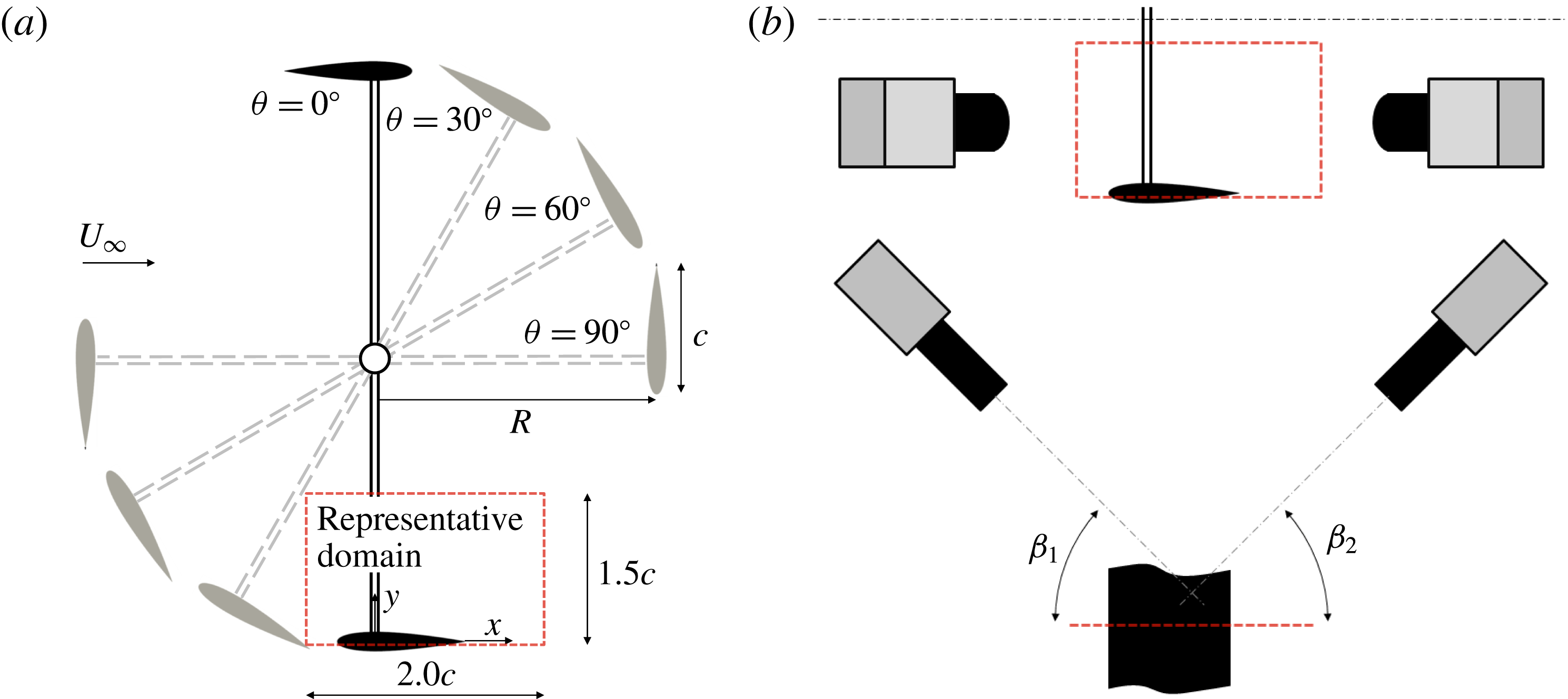
defined at the blade’s position when travelling directly upwind (figure 2).
The variation of
 $\hat{U} _{rel}$
and
 $\unicode[STIX]{x1D6FC}_{rel}$
during one cycle of rotation is shown in figure 1. We see that the amplitudes of the periodic oscillations in the local relative velocity and angle of attack diminish with increasing tip speed ratio. We expect, therefore, that at a sufficiently high tip speed ratio the flow over the blade will remain attached, and stall will not occur.
(a) Blade local relative velocity as a function of azimuthal position and tip speed ratio.
 $\unicode[STIX]{x1D703}$
is defined as per figure 2. Horizontal dashed line indicates tangential blade velocity,
 $R\unicode[STIX]{x1D6FA}$
. (b) Corresponding angle of attack.
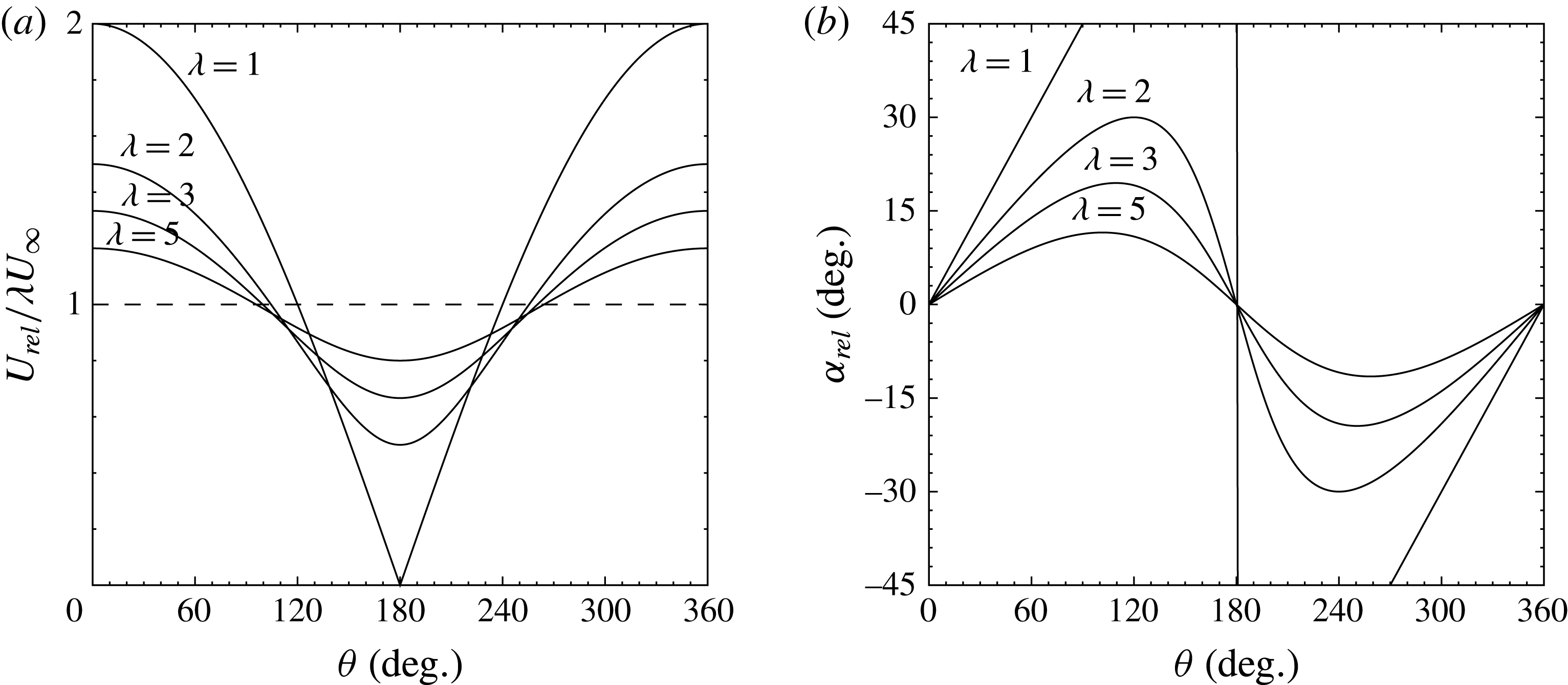
Since the oscillations in local relative velocity are centred about the tangential blade velocity,
 $R\unicode[STIX]{x1D6FA}$
, (figure 1
a) this appears to be an appropriate choice for the velocity scale when considering the blade aerodynamics. The appropriate Reynolds number used in this investigation is therefore taken to be the chord Reynolds number
 $$\begin{eqnarray}\displaystyle Re_{c}=\frac{R\unicode[STIX]{x1D6FA}c}{\unicode[STIX]{x1D708}}. & & \displaystyle\end{eqnarray}$$
The use of a constant Reynolds number is of course an approximation, given that throughout each rotation cycle the velocity relative to the turbine blades varies considerably, as given by (1.2). The simplicity of a constant Reynolds number based on the tangential velocity can aid in the tractability of the problem. This same definition of chord-based blade Reynolds number has been used previously by a variety of authors (Ferreira et al. Reference Ferreira, van Kuik, van Bussel and Scarano2009; Bachant & Wosnik Reference Bachant and Wosnik2016; Dunne, Schmid & McKeon Reference Dunne, Schmid and McKeon2016).
The pitching kinematics of vertical axis wind turbine blades differ from those considered in most of the dynamic stall literature in that the centre of rotation of the blade is offset from the blade itself, and the fundamental pitch rate,
 $\unicode[STIX]{x1D6FA}$
, of the blade is therefore related directly to the blade velocity scale,
 $\unicode[STIX]{x1D706}U_{\infty }=R\unicode[STIX]{x1D6FA}$
. The dimensionless form of the pitch rate thus reduces to
 $$\begin{eqnarray}\displaystyle K_{c}=\frac{c}{2R}, & & \displaystyle\end{eqnarray}$$
which depends only on the geometry of the turbine and can therefore be varied independently of the tip speed ratio. In addition to these parameters, the solidity ratio is necessary to fully characterise wind turbine behaviour, and although the solidity ratio is not held constant in this study (being related to the dimensionless pitching ratio for a given number of blades), its value (
 $0.2\leqslant \unicode[STIX]{x1D70E}\leqslant 0.4$
) remains in the vicinity of the optimum for wind turbines of this type (Brusca, Lanzafame & Messina Reference Brusca, Lanzafame and Messina2014).
(a) Schematic of experiment (as viewed from above), with representative measurement domain, coordinate system and geometric parameters marked. (b) Details of the camera arrangement, where the angles
 $\unicode[STIX]{x1D6FD}_{1}$
and
 $\unicode[STIX]{x1D6FD}_{2}$
both approximate
 $45^{\circ }$
for all experiments.
The occurrence and evolution of dynamic stall as it relates to these dimensionless parameters is not yet well understood. Fujisawa & Shibuya (Reference Fujisawa and Shibuya2001) presented PIV measurements of the dynamic stall of a VAWT blade at
 $\unicode[STIX]{x1D706}=1$
,
 $2$
and
 $3$
and
 $Re_{c}=3000$
, and showed that two dynamic stall events occur for each full rotation of the turbine; once on the upstream portion of the rotation, and once on the downstream portion. However, apart from the angle at which it occurred, the qualitative behaviour of the dynamic stall did not vary significantly with tip speed ratio, in agreement with the later studies by Ferreira et al. (Reference Ferreira, van Kuik, van Bussel and Scarano2009), Buchner et al. (Reference Buchner, Lohry, Martinelli, Soria and Smits2015a
) and Parker & Leftwich (Reference Parker and Leftwich2016).
As to the effects of dimensionless pitch rate, VAWT blades operate at
 $K_{c}\leqslant 0.2$
, which is low when compared to other unsteady airfoil applications, such as flapping flight or perching which typically occur in the range
 $0.2<K_{c}<0.7$
(Shyy et al.
Reference Shyy, Lian, Tang, Viieru and Liu2008). Albertson, Troutt & Kedzie (Reference Albertson, Troutt and Kedzie1988) presented force coefficients and smoke visualisations for a NACA0015 airfoil pitching at
 $K_{c}\leqslant 0.2$
, and found that a leading edge vortex was formed even at these very low pitch rates, but there were indications that further or subsequent leading edge vortices were formed after the primary vortex detached from the leading edge. Geissler & Haselmeyer (Reference Geissler and Haselmeyer2006) investigated the onset of dynamic stall in detail for an airfoil pitching at
 $K_{c}=0.073$
, and concluded that at this very low pitching rate the initiation of dynamic stall was dominated by trailing edge flow reversal. Leading edge separation and leading edge vortex formation occurred in this study only as a result of the trailing edge flow reversal reaching the leading edge. This behaviour is more often associated with static, or quasi-steady stall, and poses the question of what paradigmatic distinction can be made between static and dynamic stall for the low pitch rates encountered by VAWT blades and what, phenomenologically, distinguishes the two.
The effect of Reynolds number on massively separating flows over unsteady airfoils has been considered to be relatively minor, in that it seems to affect primarily the behaviour of the laminar separation bubble formed near the leading edge (Ol et al. Reference Ol, Bernal, Kang and Shyy2009a ) as to the timing of initial flow separation and its location on the airfoil’s surface. Although Reynolds-dependent three-dimensional transitional and turbulent effects have been shown to occur in a leading edge vortex (Garmann & Visbal Reference Garmann and Visbal2011; Buchner & Soria Reference Buchner and Soria2013; Buchner et al. Reference Buchner, Honnery and Soria2017), the mean circulation shed from an unsteady airfoil is not a function of Reynolds number (Buchner & Soria Reference Buchner and Soria2014). Although this circulation production can be predicted numerically accurately (Ramesh et al. Reference Ramesh, Gopalarathnam, Granlund, Ol and Edwards2014; Buchner et al. Reference Buchner, Lohry, Martinelli, Soria and Smits2015a ), simplified scalings and analytical relations of the sort presented by Buchholz, Green & Smits (Reference Buchholz, Green and Smits2011) remain useful since they offer physical insight, and provide a tool for estimating the behaviour of flow phenomena. Here, we address the parametric dependence and scaling of dynamic stall in vertical axis wind turbines.
2 Experiment
The
 $0.61~\text{m}\times 0.915~\text{m}$
cross-section atmospheric pressure recirculating wind tunnel at Princeton University was used to test a vertical axis wind turbine of the H-type gyromill configuration, under a range of conditions. The turbine was flow driven, with an electric motor used for starting and as a brake to hold to a desired rotational rate. This set-up avoids the complications associated with driven motor-driven turbines as outlined in Araya & Dabiri (Reference Araya and Dabiri2015a
). The test model had two NACA0015 blades of span 450 mm, and it was constructed of aluminium and carbon fibre. A two-bladed design was used so that blade interactions and solidity were minimised, whilst allowing highly resolved PIV measurements of the flow around the blades. Three sets of blades were tested, with chord lengths
 $c=50$
, 75 and 100 mm. The choice of airfoil cross-section is primarily important for the initiation of dynamic stall (Abbott & von Doenhoff Reference Abbott and von Doenhoff1959; Ramesh et al.
Reference Ramesh, Gopalarathnam, Granlund, Ol and Edwards2014) but has little effect on the post-stall behaviour of the separated flow. It was informed both by the desire for a thin airfoil exhibiting early and strong leading edge stall and to match the previous dynamic stall work of Ferreira et al. (Reference Ferreira, van Kuik, van Bussel and Scarano2009), but is not intended to be representative of optimised wind turbine blades such as those proposed by Ferreira & Geurts (Reference Ferreira and Geurts2015) and Ragni, Ferreira & Correale (Reference Ragni, Ferreira and Correale2015).
Two-camera digital stereoscopic PIV measurements (Arroyo & Greated Reference Arroyo and Greated1991; Willert & Gharib Reference Willert and Gharib1991; Keane & Adrian Reference Keane and Adrian1992; Prasad Reference Prasad2000; Raffel et al.
Reference Raffel, Willert, Wereley and Kompenhans2007) were performed in the region of the radially inwards facing surface of the turbine blade. The measurement plane lay coincident with the mid-span of turbine blades, at the centre-plane of the test section cross-section. The location of the measurement domain in relation to the turbine, and the placement of the PIV acquisition cameras is illustrated in figure 2, where the geometric parameters relevant to this experiment are also defined. An optical encoder and Arduino Nano V3.3 board were used for timing and data acquisition control, with on board data storage via Micro Secure Digital (SD) and communication via Bluetooth. The accuracy of the phase locking was determined to be
 $\pm 0.5^{\circ }$
of the commanded phase, which translates to between
 $2.2\,\%$
and
 $4.3\,\%$
of chord. Seeding was introduced into the free stream flow by an MDG brand clean nitrogen fed fog machine, producing a mean particle size of approximately
 $1~\unicode[STIX]{x03BC}\text{m}$
. One thousand PIV image pairs were acquired for each set of flow and kinematic parameters for azimuthal blade angles
 $30^{\circ }\leqslant \unicode[STIX]{x1D703}\leqslant 165^{\circ }$
, which captures most of the upstream arc of the turbine blade rotation. Considering a random PIV cross-correlation particle displacement uncertainty of
 $\unicode[STIX]{x1D716}(\unicode[STIX]{x0394}x)\approx 0.06$
pixels (Soria Reference Soria1996), the mean velocity estimate has a standard error of approximately
 $\unicode[STIX]{x1D70E}(\bar{u}_{i})=0.095\,\%$
of the free stream velocity. Assuming negligible spatial mapping error and spatially and directionally homogeneous velocity errors, the standard error for the estimate of the phase-averaged vorticity may also be derived, as
 $\unicode[STIX]{x1D70E}(c\bar{\unicode[STIX]{x1D714}}_{z}/U_{\infty })=0.50$
.
Two LaVision Imager sCMOS double shutter cameras were used, with a sensor resolution of
 $2560\times 2160$
pixels. Each camera was fitted with a 50 mm focal length lens, and had a field of view approximately
 $150\times 125~\text{mm}$
in size. The measurement domain spanned between one to three chord lengths, depending on which model was being tested, which was sufficient to capture the early time development of dynamic stall. The magnification of each camera was approximately
 $9.0$
for all measurements, giving an image resolution of
 $58.6~\unicode[STIX]{x03BC}\text{m}~\text{pixel}^{-1}$
. Images were defocussed slightly to prevent peak locking. The cameras were mounted on a turntable centred on the turbine axis to allow the rotation of the complete camera system to arbitrary azimuthal angles. The camera views were located in space, relative to one another, and dewarped using a two-plane mapping of the type proposed by Soloff, Adrian & Liu (Reference Soloff, Adrian and Liu1997).
Image pairs were cross-correlated using a multigrid algorithm (Soria Reference Soria1996), iterating from initial window dimensions of
 $64~\text{pixel}\times 64~\text{pixel}$
to a final dimensions of
 $24~\text{pixel}\times 24~\text{pixel}$
. Final interrogation windows were overlapped by
 $50\,\%$
, yielding a spatial resolution of approximately 0.7 mm per vector (
 $0.007c{-}0.014c$
per vector, depending on the model used). Prior to cross-correlation, scattered background light and spurious reflections were removed from each image pair via a high-pass filter and subtraction of the minimum intensity across the ensemble. Reflections from the turbine blade were masked. Application of a maximum displacement limit and a normalised local median filter (Westerweel & Scarano Reference Westerweel and Scarano2005) to the raw displacement vectors resulted in the rejection of
 $O(1\,\%)$
of the vectors. The velocities at the locations of the rejected vectors were interpolated from their nearest positively validated neighbours.
Data are presented for three chord-based Reynolds numbers,
 $Re_{c}=50\,000$
,
 $70\,000$
and
 $140\,000$
, realised by varying
 $\unicode[STIX]{x1D6FA}$
and
 $U_{\infty }$
together thus maintaining a constant tip speed ratio. Integer-valued tip speed ratios between
 $\unicode[STIX]{x1D706}=1$
and
 $\unicode[STIX]{x1D706}=5$
were measured, with the exact range determined for each condition depending on the extent and evolution of the structures associated with dynamic stall as well as experimental considerations including model structural integrity, optical access and free stream flow quality. Only the subset of conditions and azimuthal blade positions for which each relevant quantity can be determined from the data acquired are considered in the analysis presented here, with a focus on the strong stall phenomena observed at
 $\unicode[STIX]{x1D706}\leqslant 3$
. The dimensionless pitching rate of the turbine blades was also varied, from
 $K_{c}=0.10$
to
 $K_{c}=0.20$
, by changing the blade chord length. For each dimensionless pitch rate, the turbine angular velocity was held constant to ensure constant blade Reynolds number, while the free stream velocity was varied to change tip speed ratio. Measurements were taken at azimuthal blade angle increments of
 $15^{\circ }$
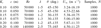
, over a range sufficient to capture the early stages of dynamic stall at each experimental condition. Table 1 lists the relevant parameters for which measurements were taken.
Parameters of the experiment, for which measurements were performed.
The free stream velocity was measured using a total pressure and static pressure ports in the wind tunnel test section, approximately two turbine diameters upstream of the model. The free stream velocity over the duration of each experiment was constant to within approximately
 $\pm 2\,\%$
when
 $U_{\infty }\geqslant 4.50~\text{m}~\text{s}^{-1}$
. Due to variability in the free stream velocity at low speeds, results obtained for
 $U_{\infty }<4.50~\text{m}~\text{s}^{-1}$
must be treated with caution, and are not presented here. This includes
 $\unicode[STIX]{x1D706}\geqslant 4$
at
 $K_{c}=0.10$
and
 $Re=50\,000$
.
3 Topology of the dynamic stall
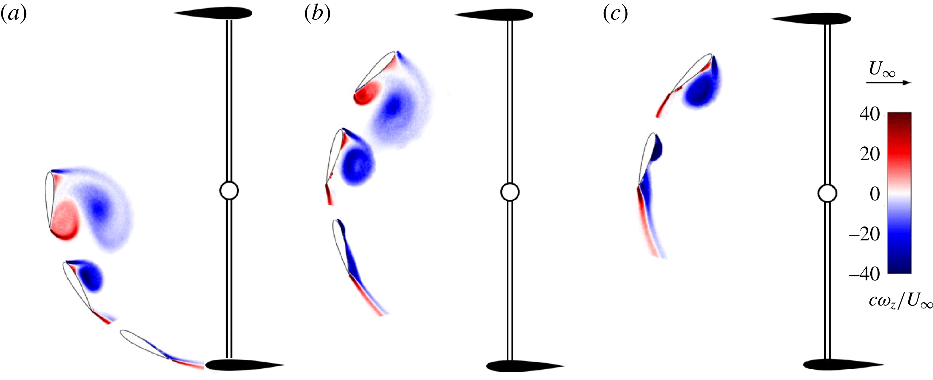
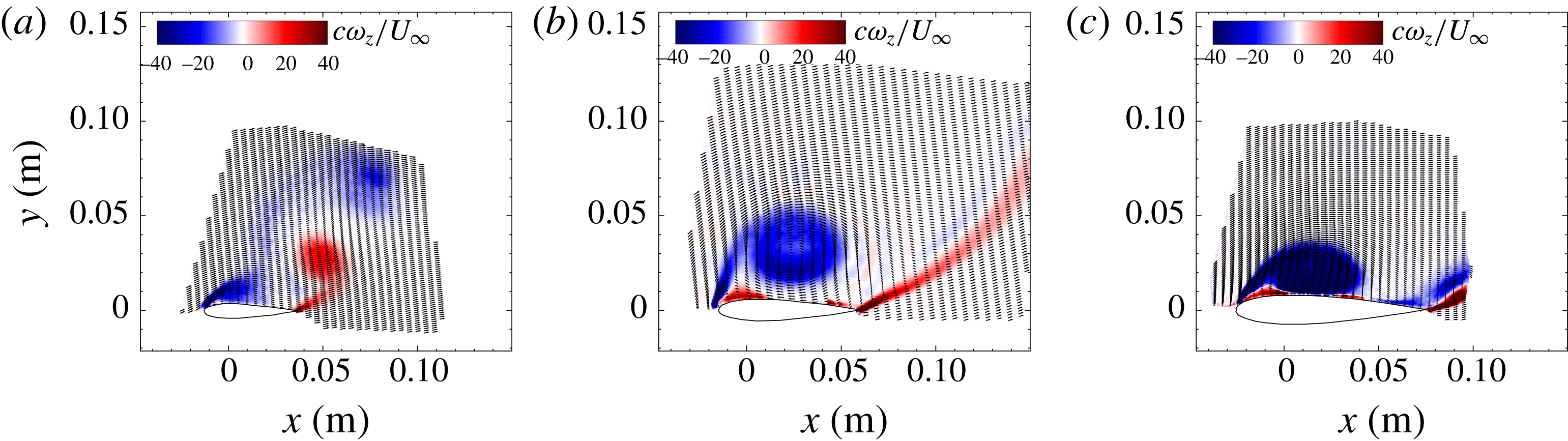
As indicated earlier, dynamic stall is characterised by the formation of a coherent vortex from the circulation shed at the leading edge of a blade or airfoil. An overview of the development of this leading edge vortex and the subsequent appearance of a trailing edge vortex is provided by contours of spanwise vorticity plotted in figure 3. The results of measurements at several selected azimuthal locations during the upstream pass of the turbine blade are given. The primary vortex structures and their morphology are clearly seen. Panels (a–c) of figure 3 relate to three different tip speed ratios, showing the delaying effect that higher tip speed ratios have on the initiation and evolution of dynamic stall. For closer inspection, experimental contours of phase-averaged spanwise vorticity are also presented in figure 4 at
 $\unicode[STIX]{x1D703}=90^{\circ }$
for three tip speed ratios;
 $\unicode[STIX]{x1D706}=1$
,
 $2$
and
 $3$
. For ease of comparison, the PIV data are transformed into the coordinates of the moving turbine blade. Although taken at the same azimuthal phase of the turbine’s rotation, the amplitude of the angle of attack oscillation experienced is reduced at higher tip speed ratios, and there is a corresponding delay in the occurrence of dynamic stall. These three vorticity fields therefore represent three different stages in the development of the dynamic stall of the blade.
Phase-averaged vorticity contours and vector fields in the vicinity of a NACA0015 vertical axis wind turbine blade, for selected tip azimuthal blade positions. The
 $Re_{c}=70\,000$
case is chosen for illustration, and
 $K_{c}=0.15$
. (a)
 $\unicode[STIX]{x1D706}=1$
; (b)
 $\unicode[STIX]{x1D706}=2$
; (c)
 $\unicode[STIX]{x1D706}=3$
.
At a tip speed ratio of
 $\unicode[STIX]{x1D706}=3$
, figure 4(c) indicates a slowing of the flow over the suction side of the blade, and a resultant thickening of the boundary layer with a small flow reversal near the trailing edge. At this point in the stall process, the flow remains attached at the leading edge, and the flow appears qualitatively similar to the incipient stages of quasi-steady type stall (Jones Reference Jones1933; Gault Reference Gault1957). At
 $\unicode[STIX]{x1D706}=2$
, shown in figure 4(b), a tight leading edge vortex has appeared, and only a vestige of flow separation is seen further downstream. At
 $\unicode[STIX]{x1D706}=1$
(figure 4
a), a large leading edge vortex dominates the suction surface of the blade and extends to approximately
 $1.5$
chords lengths above the surface of the blade, and the shear layer at the trailing edge has rolled up to form a well-defined trailing edge vortex. A contiguous region of vorticity connecting each of the leading and trailing edges to their respective vortices indicates that these vortices continue to receive circulation from the shear layers originating at the blade surface, and thus continue to grow in strength. Notably a region of vorticity, opposite in sign to the primary leading edge vortex and situated between it and the turbine blade, appears also. This secondary vorticity results from the interaction of the leading edge vortex with the no-slip condition at the airfoil surface. This phenomenon has been seen previously in studies of unsteady airfoils (Soria et al.
Reference Soria, New, Lim and Parker2003; Buchner et al.
Reference Buchner, Buchmann, Kilany, Atkinson and Soria2012), but never explicitly noted for the flow around vertical axis wind turbine blades.
It appears, therefore, that dynamic stall for typical vertical axis wind turbine operating conditions progresses from a boundary layer thickening and quasi-steady-like separation near the trailing edge (as in figure 4 c), to a sudden boundary layer separation near the leading edge and subsequent formation of a coherent leading edge vortex. The appearance of the leading edge vortex causes reattachment of the boundary layer near the trailing edge of the blade suction surface (as in figure 4 b), until at larger angles of attack the trailing edge shear layer rolls up to form a trailing edge vortex (figure 4 a).
Phase-averaged vorticity contours and vector fields in the vicinity of a NACA0015 vertical axis wind turbine blade at
 $Re_{c}=70\,000$
,
 $\unicode[STIX]{x1D703}=90^{\circ }$
and
 $K_{c}=0.15$
. (a)
 $\unicode[STIX]{x1D706}=1$
; (b)
 $\unicode[STIX]{x1D706}=2$
; (c)
 $\unicode[STIX]{x1D706}=3$
.

The effect of dimensionless pitch rate
 $K_{c}$
on the evolution of dynamic stall is also important. Figure 5 illustrates the dynamic stall behaviour at
 $\unicode[STIX]{x1D703}=105^{\circ }$
and
 $\unicode[STIX]{x1D706}=2$
for three different pitch rates. The primary effect of increasing pitch rate on the leading edge vortex is to reduce its spatial growth relative to the chord length of the blade, which is consistent with the results of previous studies of pitching plates undergoing dynamic stall (Ol, Eldredge & Wang Reference Ol, Eldredge and Wang2009b
). At higher dimensionless pitch rates the leading edge vortex appears tighter and sits closer to the blade’s surface, and there are indications that secondary vorticity is formed between the blade and the leading edge vortex.
We are interested in how these flow patterns relate to turbine performance. In figure 5(a), where
 $K_{c}=0.10$
, a prominent trailing edge vortex has formed and it interacts with the leading edge vortex in such a way as to deform and elongate it. The peak vorticity in the leading edge vortex in this case has moved approximately two chord lengths away from the blade, and a second distinct leading edge vortex is beginning to form. This behaviour is seen to occur in all
 $K_{c}=0.10$
cases, but not for cases with larger values of
 $K_{c}$
. This result is significant because it is the movement of the circulation away from the blade that causes a loss of aerodynamic force on the blade. There is some uncertainty as to the precise definition of ‘shedding’ of a vortex, with various definitions proposed, based on the finite time Lyapunov exponents (Haller Reference Haller2005; Green, Rowley & Smits Reference Green, Rowley and Smits2011), among other criteria. Here it is however in general clear that the cessation of circulation addition into the leading edge vortex and its movement away from the airfoil coincides closely with a loss of its contribution to the airfoil lift. It appears that there is a parametric threshold above which this behaviour is triggered. The following sections explore the reasons for this behaviour.
Phase-averaged vorticity contours and vector fields in the vicinity of a NACA0015 vertical axis wind turbine blade at
 $Re_{c}=70\,000$
,
 $\unicode[STIX]{x1D703}=105^{\circ }$
,
 $\unicode[STIX]{x1D706}=2$
. (a)
 $K_{c}=0.10$
, (b)
 $K_{c}=0.15$
, (c)
 $K_{c}=0.20$
.
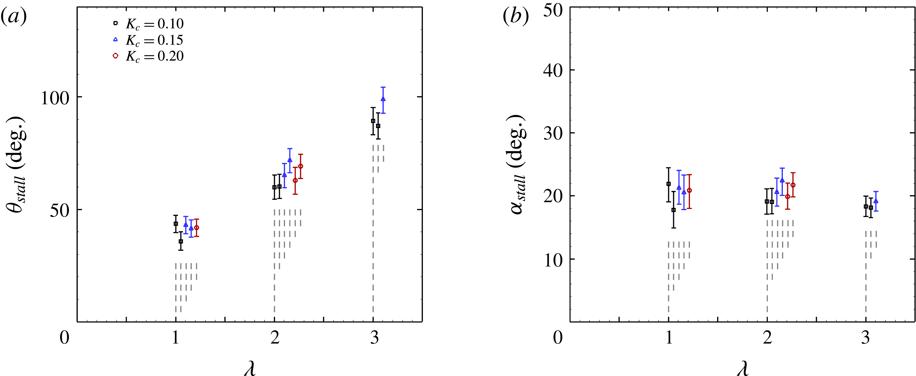
(a) Azimuthal stall angle (angle at which leading edge vortex first appears); (b) relative angle of attack at stall. For clarity, where error bars overlap one another data points have been arbitrarily horizontally displaced, as indicated by the vertical grey dashed lines. Multiple data points of the same colour/symbol relate to various Reynolds numbers.
4 Stall timing
The leading edge vortex first forms at a particular azimuthal angle,
 $\unicode[STIX]{x1D703}_{stall}$
, the variation of which with tip speed ratio is shown in figure 6(a). The stall angle was determined by fitting a polynomial to the growth of circulation in the leading edge vortex as a function of azimuthal angle, and estimating its
 $x$
-intercept, with error bars defined as the uncertainty of this intercept estimate due to the propagated velocity measurement uncertainty. We see that tip speed ratio strongly affects the timing (or azimuthal location) of leading edge stall, with increased values of
 $\unicode[STIX]{x1D706}$
acting to delay its occurrence. When the transformation of
 $\unicode[STIX]{x1D703}_{stall}$
to the relative angle of attack,
 $\unicode[STIX]{x1D6FC}_{stall}$
is made (as in figure 6
b), it becomes clear that across the tip speed ratio range measured here, and within the measurement precision, the stall angle of attack is approximately constant at a value between
 $18^{\circ }$
and
 $23^{\circ }$
, much larger than the static stall angle at comparable Reynolds numbers, which is approximately
 $10^{\circ }$
(Abbott & von Doenhoff Reference Abbott and von Doenhoff1959). Figure 6 also shows that the dimensionless pitch rate has little effect on the timing of the leading edge vortex formation, since the azimuthal angle and angle of attack at which the leading edge vortex first appears do not vary with dimensionless pitch rate.
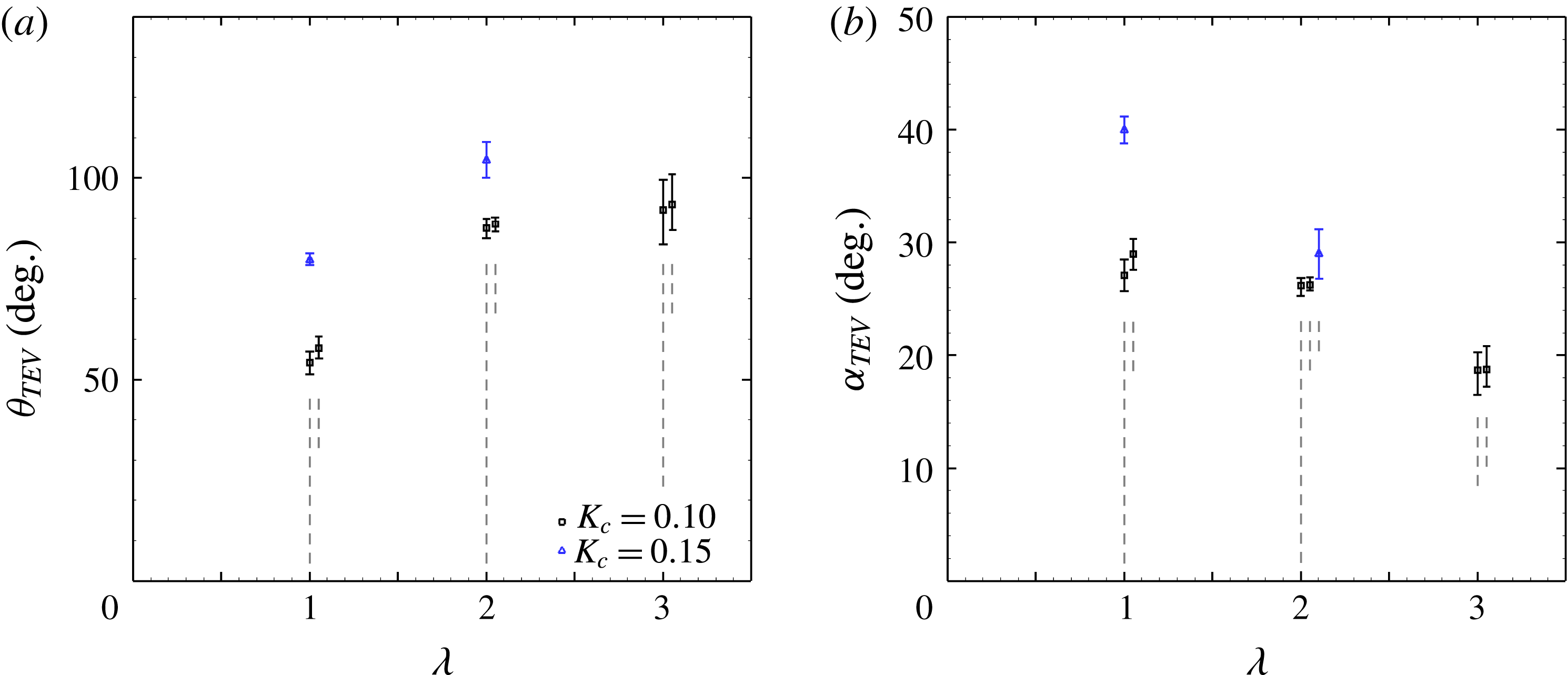
Another consideration is the timing of the formation of the trailing edge vortex (TEV). Figures 7(a) and 7(b) display the azimuthal angle
 $\unicode[STIX]{x1D703}_{TEV}$
and relative angle of attack
 $\unicode[STIX]{x1D6FC}_{TEV}$
, respectively, at which the trailing edge shear layer first rolls up into a trailing edge vortex. The trends with
 $\unicode[STIX]{x1D706}$
and
 $K_{c}$
are not as straight forward as for the leading edge vortex (LEV). The azimuthal angle does not simply increase with
 $\unicode[STIX]{x1D706}$
, nor is the relative angle of attack constant. Unlike the formation of the leading edge vortex, the trailing edge vortex formation also appears to depend on dimensionless pitch rate,
 $K_{c}$
; it appears that at
 $K_{c}=0.15$
the TEV forms later than at
 $K_{c}=0.10$
, and this difference is more pronounced at lower tip speed ratios. When the dimensionless pitch rate is increased to
 $K_{c}=0.20$
, no TEV is observed in these experiments.
Angle
 $\unicode[STIX]{x1D703}_{TEV}$
at which the trailing edge shear layer rolls up to form a trailing edge vortex, plotted against the tip speed ratio,
 $\unicode[STIX]{x1D706}$
. (a) Azimuthal angle; (b) relative angle of attack when TEV first appears. For clarity, where error bars overlap one another data points have been arbitrarily horizontally displaced, as indicated by the vertical grey dashed lines. Multiple data points of the same colour/symbol relate to various Reynolds numbers.
The variation of
 $\unicode[STIX]{x1D703}_{TEV}$
and
 $\unicode[STIX]{x1D6FC}_{TEV}$
with
 $\unicode[STIX]{x1D706}$
and
 $K_{c}$
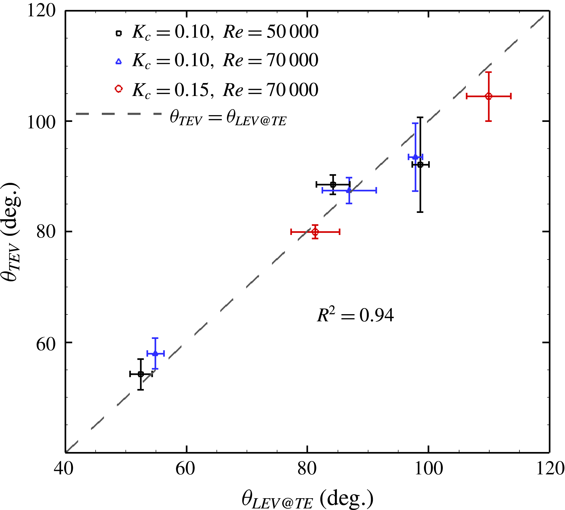
can be explained by the interaction of the LEV with the trailing edge. The bounds of the LEV were defined by a contour of vorticity twice the standard deviation of the vorticity in the irrotational areas of the mean flow, with the positional error of this contour estimated by a similar procedure as for the uncertainty in the stall angle. The azimuthal angle at which the growth of the LEV leads to its downstream extent passing the position of the trailing edge is then determined. There exists a strong correlation (
 $R^{2}=0.94$
) between this angle and the angle of formation of the trailing edge vortex (see figure 8). It appears that as the downstream extent of the LEV extends past the trailing edge, the trailing edge shear layer is perturbed by the reverse flow induced by the leading edge vortex, causing the shear layer to roll up and form the trailing edge vortex.
Angle
 $\unicode[STIX]{x1D703}_{TEV}$
at which the trailing edge shear layer rolls up to form a trailing edge vortex, plotted against the azimuthal angle
 $\unicode[STIX]{x1D703}_{LEV@TE}$
at which the downstream extent of the leading edge vortex reaches the position of the trailing edge.
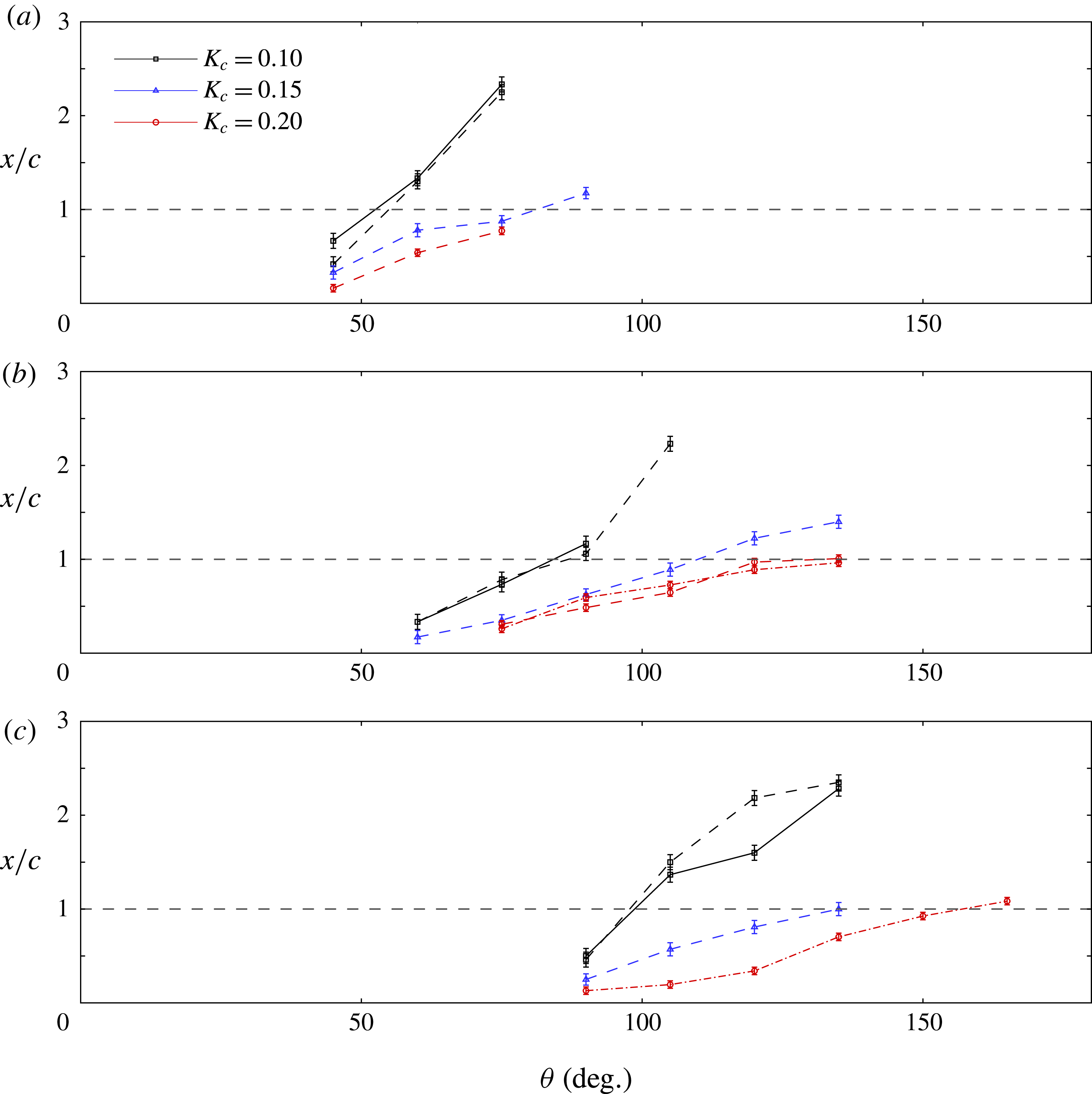
How does the growth of the LEV depend on the VAWT blade kinematics? In figure 9, the downstream extent of the LEV is plotted against azimuthal angle for all tip speed ratios and dimensionless pitch rates. The horizontal dashed line marks the location of the trailing edge. Consistent with the delayed formation of the LEV as a function of
 $\unicode[STIX]{x1D706}$
, so too is its spatial growth delayed. Despite pitch rate having little effect on the LEV stall angle, we see that at lower values of
 $K_{c}$
the LEV spatial growth becomes more rapid. This behaviour is consistent with that observed in the example vorticity fields given in figure 5.
Growth of the maximum streamwise extent of the leading edge vortex with azimuthal angle
 $\unicode[STIX]{x1D703}$
. (a)
 $\unicode[STIX]{x1D706}=1$
; (b)
 $\unicode[STIX]{x1D706}=2$
; (c)
 $\unicode[STIX]{x1D706}=3$
. Solid lines indicate
 $Re=50\,000$
, dashed lines
 $Re=70\,000$
and dot-dash lines
 $Re=140\,000$
. The horizontal thick dashed line indicates the trailing edge location.
5 Scaling the production of circulation
Now that the circumstances under which dynamic stall occurs have been established, and its timing has been determined, we address the behaviour of the stall after the initiation of leading edge flow separation. Of primary importance is understanding the rate of growth of the circulation,
 $\unicode[STIX]{x1D6E4}$
, within the leading edge vortex.
Ramesh et al. (Reference Ramesh, Gopalarathnam, Granlund, Ol and Edwards2014) showed that the circulation shed from an unsteady airfoil can be predicted based on the rate of change of bound circulation associated with the airfoil, since any changes in bound circulation must be balanced by shedding circulation. This works well for kinematics in which the flow remains attached at the leading edge. When a leading edge vortex is formed however, the relative apportionment of shed circulation into the leading and trailing edge vortices depends on empirical knowledge of the suction that can be maintained at the leading edge. Here we seek a more explicit parametric scaling.
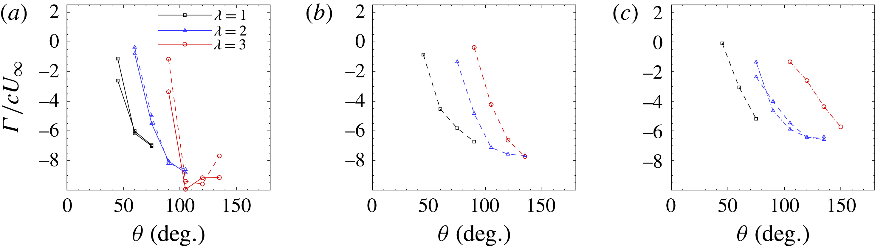
The phase-averaged circulation in the leading edge vortex is shown as a function of azimuthal angle in figure 10. Each subplot shows the circulation for a particular dimensionless pitch rate, for tip speed ratios of
 $1$
,
 $2$
and
 $3$
, and Reynolds numbers of
 $50\,000$
,
 $70\,000$
and
 $140\,000$
. The circulation values are all normalised by the chord length and free stream velocity as
 $\hat{\unicode[STIX]{x1D6E4}}=\unicode[STIX]{x1D6E4}/cU_{\infty }$
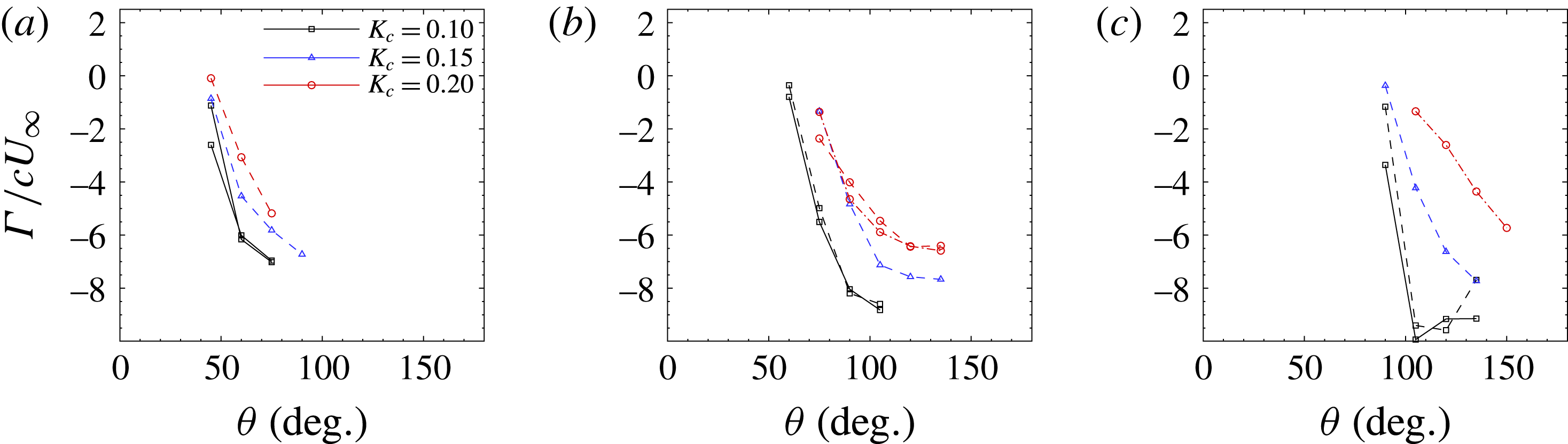
. In general, the post-separation rate of LEV circulation growth is initially high, with a gradual reduction as the stall progresses, and we see the delayed initiation of stall as the tip speed ratio is increased. Figure 11 shows the same data, but each subplot contains values at a single tip speed ratio. It is clear that the dimensionless pitch rate affects the rate of leading edge vortex circulation addition, albeit not as strongly as does the tip speed ratio. This circulation addition rate is lower at higher dimensionless pitching rates, and the variation is greater at higher tip speed ratios. Extrapolating the circulation curves back to
 $\hat{\unicode[STIX]{x1D6E4}}=0$
, the circulation data appear to be consistent with our earlier observation that the stall angle is not significantly affected by the dimensionless pitch rate.
Phase-averaged normalised circulation in the leading edge vortex for different tip speed ratios. (a)
 $K_{c}=0.10$
, (b)
 $K_{c}=0.15$
, (c)
 $K_{c}=0.20$
. Solid lines indicate
 $Re=50\,000$
, dashed lines
 $Re=70\,000$
and dot-dash lines
 $Re=140\,000$
.
Phase-averaged normalised circulation in the leading edge vortex for different pitch rates. (a)
 $\unicode[STIX]{x1D706}=1$
; (b)
 $\unicode[STIX]{x1D706}=2$
; (c)
 $\unicode[STIX]{x1D706}=3$
. Solid lines indicate
 $Re=50\,000$
, dashed lines
 $Re=70\,000$
and dot-dash lines
 $Re=140\,000$
.
We find that subtracting the stall angle,
 $\unicode[STIX]{x1D703}_{stall}$
, from the azimuthal angle,
 $\unicode[STIX]{x1D703}$
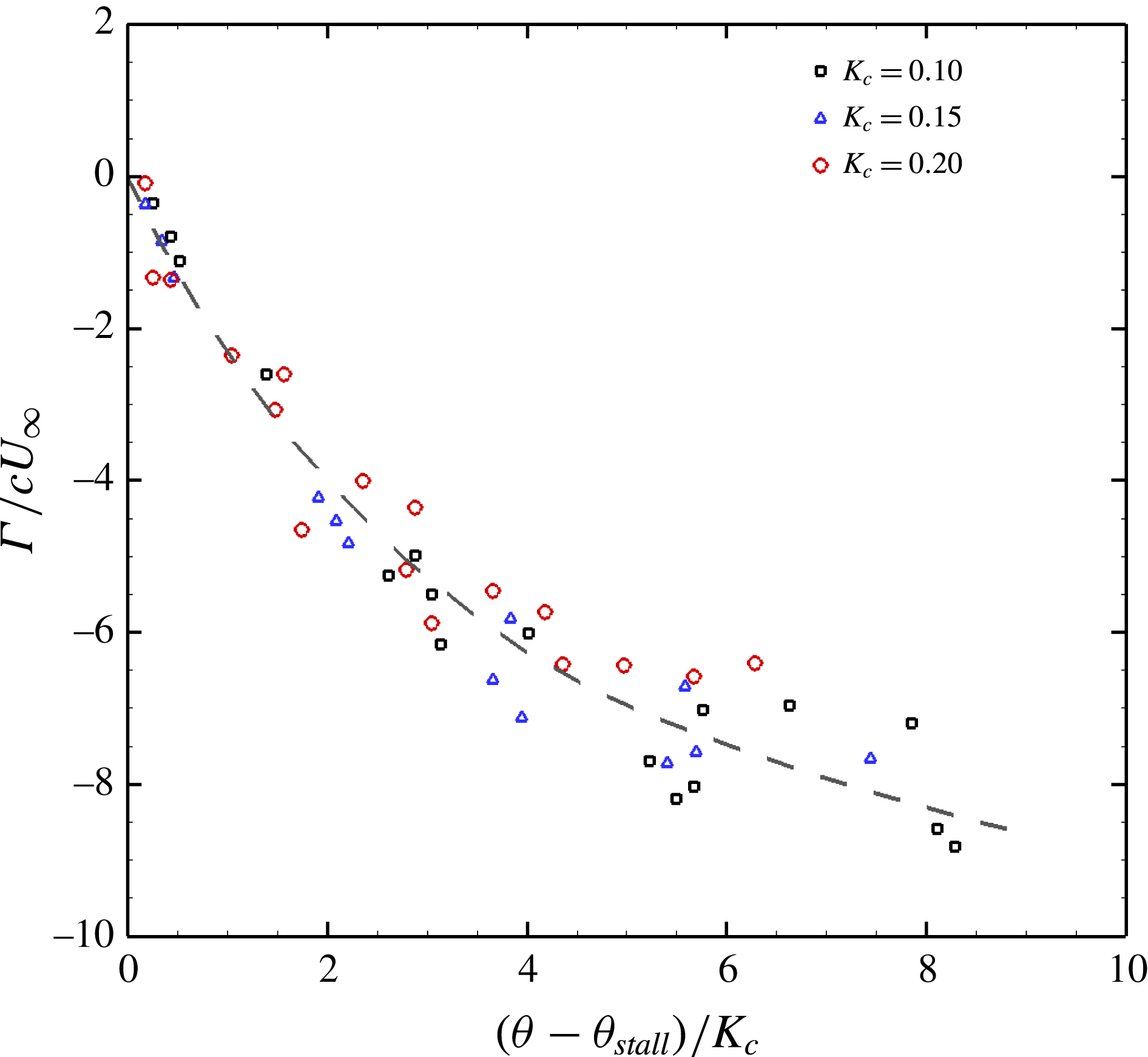
, collapses the circulation data at any given tip speed ratio (not shown here). This scaling does not, however, account for the observed variation with pitch rate. Adjusting for the effect of pitch rate requires identifying the appropriate time scale of the vortex growth.
It should be recognised that all the circulation shed from the leading edge post-stall has its genesis in the shear layer imposed due to no-slip at the leading edge of the blade. The velocity differential at the leading edge is
 $O(U_{\infty })$
. It might be expected therefore that per unit length along the blade’s surface, the circulation produced at the leading edge scales according to
 $$\begin{eqnarray}\displaystyle & \displaystyle \unicode[STIX]{x0394}\unicode[STIX]{x1D6E4}\sim U_{\infty }\unicode[STIX]{x0394}x\sim U_{\infty }R\unicode[STIX]{x0394}\unicode[STIX]{x1D703} & \displaystyle\end{eqnarray}$$
since
 $\unicode[STIX]{x0394}x$
equates to the tangential distance travelled by the blade,
 $R\unicode[STIX]{x0394}\unicode[STIX]{x1D703}$
. We expect, therefore, that
 $$\begin{eqnarray}\displaystyle & \displaystyle \hat{\unicode[STIX]{x1D6E4}}=\frac{\unicode[STIX]{x1D6E4}}{cU_{\infty }}\sim \frac{R}{c}\int _{\unicode[STIX]{x1D703}_{stall}}^{\unicode[STIX]{x1D703}}\,\text{d}\unicode[STIX]{x1D703} & \displaystyle\end{eqnarray}$$
so that
 $$\begin{eqnarray}\displaystyle & \displaystyle \hat{\unicode[STIX]{x1D6E4}}=\frac{\unicode[STIX]{x1D6E4}}{cU_{\infty }}\sim \frac{1}{K_{c}}(\unicode[STIX]{x1D703}-\unicode[STIX]{x1D703}_{stall}). & \displaystyle\end{eqnarray}$$
Figure 12 demonstrates that the data agree well with this basic scaling, and although the relationship is nonlinear it seems clear that the production of circulation at the leading edge is governed by the post-stall distance travelled by the blade about the circumference of the turbine.
Production of circulation in the leading edge vortex showing the collapse across all dimensionless pitch rates and tip speed ratios when scaled based on the dimensionless pitch rate.
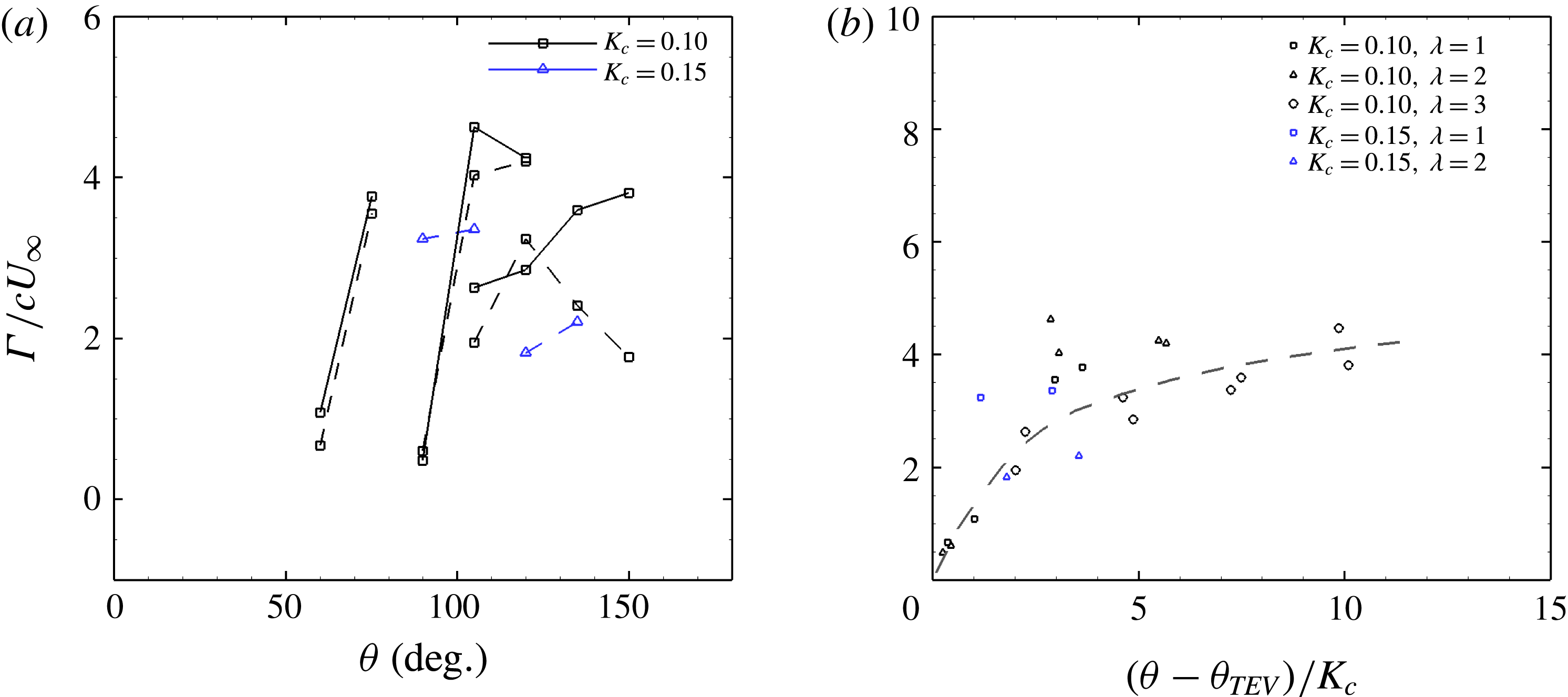
With respect to the trailing edge vortex, since the TEV appears later than the leading edge vortex, there were fewer measurements available for the circulation in the trailing edge vortex. The results are presented in figure 13(a) as a function of the azimuthal angle. The circulation is normalised in the same way as for the leading edge vortex, using the chord length and the free stream velocity. Based on these limited data it appears that the TEV circulation behaves similarly to the LEV circulation, with azimuthal delays being induced by increases in both tip speed ratio and dimensionless pitching rate. In figure 13(b) the same scaling has been applied to these data as was developed for the leading edge circulation data. The collapse with this scaling looks promising.
(a) The growth of circulation in the trailing edge vortex with azimuthal angle. (b) Scaled TEV circulation. Solid lines indicate
 $Re=50\,000$
, dashed lines
 $Re=70\,000$
and dot-dash lines
 $Re=140\,000$
.
6 Vortex interaction and shedding
As indicated by the vorticity fields in figure 5, the shape and extent of the leading edge vortex is strongly affected by the value of the dimensionless pitching rate. At high dimensionless pitching rate,
 $K_{c}=0.2$
, the leading edge vortex remains compact in the region over the suction surface of the turbine blade. In contrast, the measurements at
 $K_{c}=0.1$
show a rapid stretching of the leading edge vortex away and aft of the blade, with subsequent formation of a second leading edge vortex. The time scale of circulation production in the LEV, as proposed in § 5, is consistent with the concept of optimal vortex formation (Gharib, Rambod & Shariff Reference Gharib, Rambod and Shariff1998; Dabiri Reference Dabiri2009), further adding to the evidence of its universality even for complex geometries (Domenichini Reference Domenichini2011; O’Farrell & Dabiri Reference O’Farrell and Dabiri2014). Under the optimal vortex formation framework, one would expect the LEV to shed when
 $\hat{T}=(\unicode[STIX]{x1D703}-\unicode[STIX]{x1D703}_{stall})/K_{c}\approx 8$
, a condition reached only late in the rotation of the turbine, at a time when the angle of attack is once again diminishing. The rapid aft movement and shedding of the LEV, and its variation with dimensionless pitching rate, must therefore be otherwise governed. Figure 8 demonstrates that this behaviour coincides approximately with the formation of the trailing edge vortex, and it is the interaction between the leading and trailing edge vortices that modulates the LEV evolution in this way.
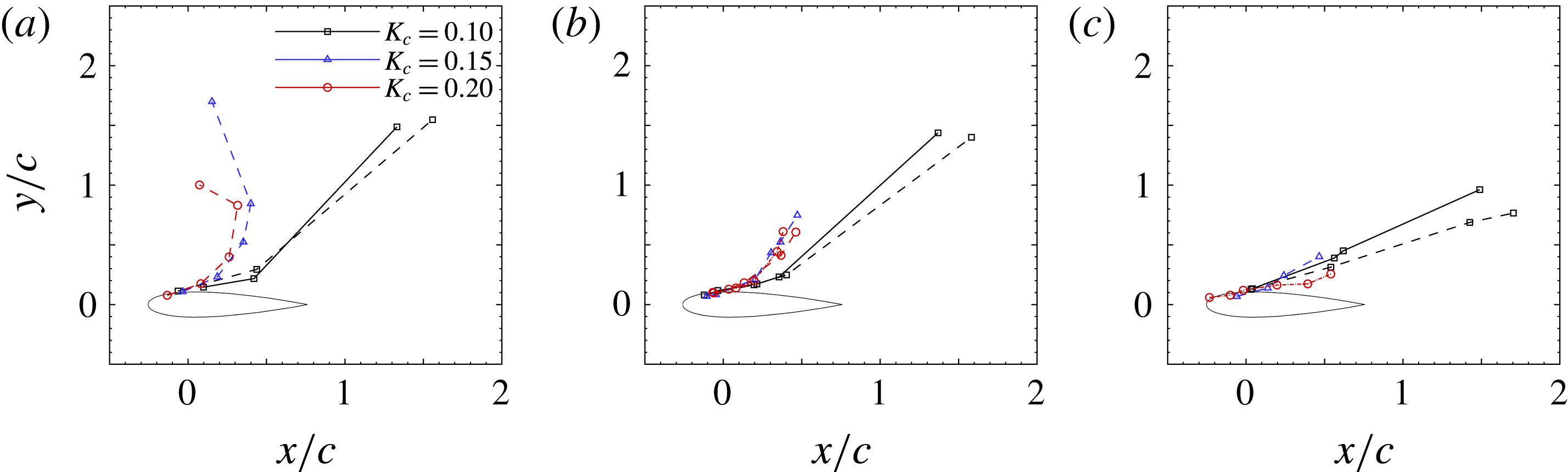
This effect can be quantified by tracking the core of the leading edge vortex as it convects away from the turbine blade. The location of the core was defined as the geometric centroid of the contiguous region of same-sign vorticity, weighted by the value of the vorticity. The path taken by the leading edge vortex is plotted in figure 14 for different tip speed ratios and dimensionless pitching rates.
Post-stall, as the blade recedes from the oncoming free stream, one might expect that at
 $\unicode[STIX]{x1D706}=1$
the shed vortices would convect downstream at about the same streamwise speed as the blade. Indeed, this is observed in the case of
 $K_{c}=0.15$
and
 $K_{c}=0.20$
. The leading edge vortex initially grows close to the plate’s upper surface before moving away in a direction almost normal to the chord line. As the dimensionless pitch rate is decreased however, the leading edge vortex instead travels rapidly aft of the blade, due to increased interaction with the trailing edge vortices. This same trend is observed for
 $\unicode[STIX]{x1D706}=2$
and
 $3$
, except that the
 $y$
-component of the LEV motion is smaller owing to the greater tip speed ratio.
Motion paths of the leading edge vortex, showing variation with dimensionless pitch rate. (a)
 $\unicode[STIX]{x1D706}=1$
; (b)
 $\unicode[STIX]{x1D706}=2$
; (c)
 $\unicode[STIX]{x1D706}=3$
. Solid lines indicate
 $Re=50\,000$
, dashed lines
 $Re=70\,000$
and dot-dash lines
 $Re=140\,000$
.
Motion paths of the leading edge vortex showing variation with tip speed ratio. (a)
 $K_{c}=0.10$
, (b)
 $K_{c}=0.15$
, (c)
 $K_{c}=0.20$
. Solid lines indicate
 $Re=50\,000$
, dashed lines
 $Re=70\,000$
and dot-dash lines
 $Re=140\,000$
.
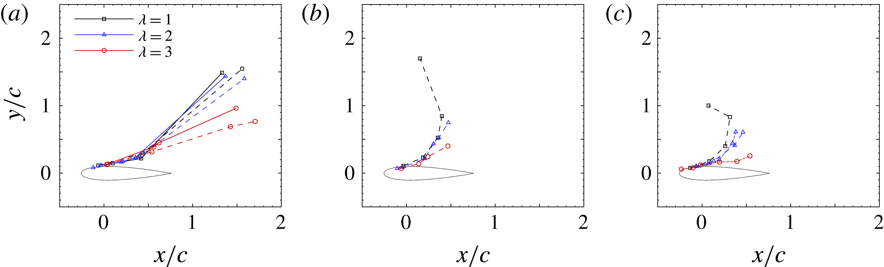
Figure 15 shows the same data as in figure 14, but plotted for different tip speed ratios. For at least the early evolution of the dynamic stall, the tip speed ratio has little effect on the
 $x$
-location of the leading edge vortex. The primary effect of tip speed ratio on the leading edge vortex’s path is to vary the distance travelled in the
 $y$
-direction.
Prior to the formation of a trailing edge vortex, the rotation of the leading edge vortex causes the outer flow to reattach to the suction surface of the blade aft of the LEV’s position, and the Kutta condition remains satisfied. Once a TEV forms however, the flow induced by each of these vortices interact, while the Kutta condition is satisfied by the TEV.
The trajectory of each of the leading and trailing edge vortices should be affected by the induced velocity due to the other, and if they are different strength they should mutually co-orbit. Since the LEV is of greater strength than the TEV, the vortex pair should rotate in the same sense as the LEV’s rotation. The presence of the blade means that the action of the LEV is such that it should force the TEV towards the blade’s surface. If we consider instead the TEV to be approximately fixed in space at the trailing edge, the LEV will orbit around its location. Considering the LEV and TEV as idealised point vortices, with rotational velocity,
 $u_{\unicode[STIX]{x1D703}}=\unicode[STIX]{x1D6E4}/2\unicode[STIX]{x03C0}r$
, given as a function of the vortices’ circulation and radial position, the induced velocity of the LEV about the trailing edge should scale simply as
 $$\begin{eqnarray}\displaystyle & \displaystyle u_{LEV}\sim \frac{1}{2\unicode[STIX]{x03C0}d}(\unicode[STIX]{x1D6E4}_{LEV}+\unicode[STIX]{x1D6E4}_{TEV}), & \displaystyle\end{eqnarray}$$
where
 $d$
is the straight line distance between the vortex cores.
Rate of variation of the leading edge vortex position with changes in the dimensionless pitching rate, as a function of the post-stall azimuthal angle. The prediction from a simple two-vortex interaction model is indicated by the grey dashed line. Error bars represent the uncertainty in the stall angle.
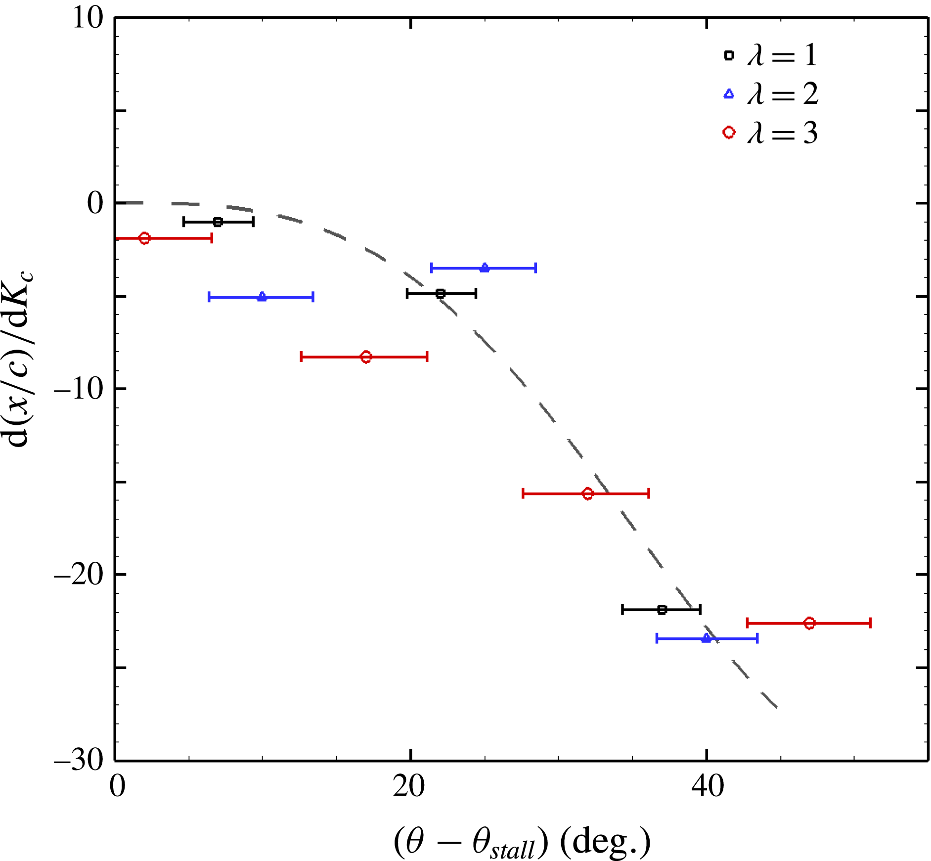
The motion predicted by this idealised vortex model does not account for the effects of the free stream velocity component or the wake of the turbine blades. To compare, therefore, the predicted motion with the motion of the LEV from the measurement, only differential quantities may be examined. The rate of change of the
 $x$
-location of the leading edge vortex with changes in the dimensionless pitch rate is calculated from the three dimensionless pitch rate cases measured using second-order central finite differences. Where multiple Reynolds numbers have been measured, the results have been averaged. These values are plotted for each tip speed ratio in figure 16. The effect of reducing the dimensionless pitch rate is to increase the
 $x$
-location of the leading edge vortex at any given angle post-stall. This result is consistent with the topology variation observed in figure 5 and the LEV tracks presented in figure 14. The dashed line represents the effect of dimensionless pitch rate on the LEV
 $x$
-location as predicted from the two-vortex model. Despite the simplicity of this model, it matches the magnitude and slope of the data well, and demonstrates that the observed topological effect of dimensionless pitch rate can be accounted for purely by this leading–trailing edge interaction, for the range of conditions tested.
7 Conclusions
Experiments were conducted to examine the topology and scaling of dynamic stall in vertical axis wind turbines over a range of industrially relevant operational parameters. This particular problem, while of course industrially relevant, is also of fundamental physical interest due to the inherent coupling of the pitch rate and blade-relevant velocity scales.
It was found that the tip speed ratio primarily governs the timing of the initiation of leading edge flow separation; increasing tip speed ratio tends to delay the azimuthal angle at which a leading edge vortex forms. The total dimensional circulation ultimately shed into the leading edge vortex also reduces with tip speed ratio, consistent with the increased dominance at high tip speed ratios of the tangential velocity of the blade over the free stream velocity component, and thus the smaller variation in angle of attack at these tip speed ratios. Above a tip speed ratio of approximately
 $3$
to
 $3.5$
, no leading edge separation is observed and no leading edge vortex forms.
It was shown that tip speed ratio alone is insufficient to fully describe the dynamic stall behaviour. The total circulation of the leading edge vortex was found to scale with the free stream velocity and the chord length of the turbine blades, but an adjustment to the time scale over which this occurs is necessary to account for pitch rate effects. The rate of accumulation of circulation in the leading edge vortex depends on the post-stall azimuthal distance travelled by the turbine blades, which can be expressed directly as a function of the dimensionless pitch rate. The circulation production and shedding behaviour is consistent across the range of Reynolds numbers tested here, with Reynolds number appearing to play only a minor role.
The stall topology was found to be significantly affected by changes in the dimensionless pitching rate. The spatial extent of the leading edge vortex varies inversely with pitching rate. Since the timing of the formation of a trailing edge vortex was found to be associated with the passage of the leading edge vortex past the trailing edge, greater spatial growth of the leading edge vortex at lower pitch rates has the effect of forcing an earlier and stronger interaction between the leading and trailing edge vortices. The interaction of these vortices induces the leading edge vortex to pinch off from the blade at an earlier azimuthal position, and a second leading edge stall vortex to form. This phenomenon has a significant effect on the overall velocity field and may have implications for the timing and severity of stall-related loss of lift of turbine blades.
Acknowledgement
This research was supported by the Australian-American Fulbright Commission and the Princeton University’s Andlinger Center for Energy and the Environment.



