1 Motivation
This paper is concerned with first steps in establishing a fully self-consistent description of a developed liquid layer passing the trailing edge of a horizontal plate, with gravity acting in vertical direction and with surface tension at play. Although this is a fundamental problem of far-reaching importance, such an analysis has not yet been presented. The problem is often associated with the existence of a hydraulic jump over the plate with the flow controlled by conditions at the trailing edge. The Froude numbers considered in the bulk of this paper preclude the formation of the jump, and we concentrate on the flow conditions at the trailing edge and demonstrate how these still impact the entire flow field. A noteworthy leap forward was Higuera’s seminal work (Higuera Reference Higuera1994) on hydraulic jumps smoothed by viscosity within the shallow-water limit. Specifically, a distinguished horizontal reference length scales with the Reynolds number, and the Froude number is finite so that variations in hydrostatic pressure are active in driving the horizontal fluid motion. Higuera (Reference Higuera1994) demonstrated that the necessary scale shortening near the plate edge, which he enforces by simply imposing there an expansive singularity, inherent in the reduced equations, had an upstream influence that fixed the position and strength of the jump. Taken in conjunction with the work of Bowles & Smith (Reference Bowles and Smith1992), which describes the onset of the jump through an initial exponential upstream tail by virtue of a viscous–inviscid interaction mechanism, Higuera’s (Reference Higuera1994) work laid the foundation for a rigorous description of the jump phenomenon. His results show that at small values of the global Froude number the jump is shifted upstream where the local Froude number is large and the structure described by Bowles & Smith (Reference Bowles and Smith1992) clearly emerges.
The trailing-edge singularity poses a downstream condition that closes the shallow-water problem, elliptic for finite Froude numbers, in a correct and unique manner. As a consequence, the flow is found to be critical at the edge (Higuera Reference Higuera1994). Remarkably, the same singularity controls Fanno flow of a regular gas choking at the orifice (Higuera & Liñán Reference Higuera and Liñán1993). As this flow might undergo a shock further upstream, we may identify a gas-dynamical analogy to the free-surface flow past a trailing edge, inevitably exhibiting a hydraulic jump. Given Higuera’s singularity, the film height at the edge is part of the solution of the shallow-water problem. Interestingly, other authors (Duchesne, Lebon & Limat Reference Duchesne, Lebon and Limat2014; Rojas & Tirapegui Reference Rojas and Tirapegui2015, see references therein) propose a terminal state directly obtained from applying the lubrication limit to the downstream portion of the jump. In the first of these studies, this is shown to become singular when the terminal film height, representing a missing ingredient to the theory, is considered as negligibly small. A nearly uniform value (
 ${\approx}0.33$
) found experimentally of the local Froude number characterising the flow immediately downstream of a pronounced jump then allows for predicting its position. Here the following deserves notation. At first, Higuera (Reference Higuera1994) demonstrated that in a singular limit associated with a vanishingly small Froude number the lubrication approximation indeed governs the downstream tail of the correspondingly strong jump, where a short region exhibiting a quiescent recirculating flow initiates its internal structure. However, that singularity is then modified so abruptly by inertial effects that Higuera’s original one, indicating the plate, edge is still met. Secondly, as he pointed out (Higuera Reference Higuera1994, p. 75), the solution to the shallow-water problem intrinsically terminates at some finite horizontal distance in the form of the latter as the former inhibits the attainment of the lubrication balance, i.e. of fully developed flow.
Also, Higuera (Reference Higuera1994) briefly considered a two-layer viscous–inviscid interaction process to reveal how the influence of streamline curvature due to momentum transport across the film, i.e. the finiteness of the film depth or the associated Reynolds number, and of surface tension locally modifies the flow near the plate edge. However, this does not address the details of the abrupt removal of the no-slip condition there. Additionally, his analysis ceases to be uniformly valid for sufficiently large Froude numbers as perfectly supercritical shallow-water flow exhibits no singularity at all – or perhaps one of a different form when instead perturbed by the effect of streamline curvature, including the capillary influence. It is unclear therefore how the flow becomes critical at the trailing edge as the Froude number is decreased. Consequently, the currently available analysis of a viscous film passing a trailing edge must be viewed as unsatisfactory and, without doubt, requires completion.
In the present paper, we tackle this challenge by a rigorous asymptotic approach. To this end, we take the effects of gravity and surface tension as suitably small compared to those of inertia and viscosity. Particular emphasis is placed on a thorough understanding of the flow very close to the edge. Focussing on asymptotically large Froude numbers, we identify a local viscous–inviscid interaction at the edge which acts to reduce the weak hydrostatically generated component of the pressure above and close to the plate to zero so as to effect the adjustment to zero excess pressure downstream of the edge. Although the flow with these parameters does not exhibit a hydraulic jump, we are able to show in detail how the upstream influence of how the flow negotiates the trailing edge is felt, through irregular, exponentially small perturbations, throughout the flow field. These are analogous to the eigensolutions that may develop nonlinearly into an identifiable hydraulic jump at lower Froude numbers in Higuera’s (Reference Higuera1994) analysis. Our work serves as a basis for subsequently completing his theory: we consider the effects of reducing the Froude number in a forthcoming study.
This paper is organised as follows. The statement of the full problem (§ 2) is succeeded by a comprehensive analysis of the flow sufficiently far away from the edge (§ 3). As an intriguing novelty, we consider both regular and the aforementioned irregular perturbations to the underlying balance of inertia and viscosity, due to relatively weak influences of gravity and streamline curvature. The irregular ones are found to originate in a viscous–inviscid interaction, and vitally here we are able to identify how their exponential growth within the entire attached flow is able to initiate strong nonlinear viscous–inviscid interaction straddling the edge (§ 3.2.2). In appendix A, we focus on the generalisation of this linear precursor to full interaction, then applying to Froude numbers smaller than those considered in the remainder of our present work. As a central part of this, next a first analytical/numerical investigation of the strong interaction process is put forward (§ 4). Throughout, the impact of surface tension is identified. Finally, we sketch the pathway to the emergence of Higuera’s singularity and the resolution of the associated discrepancy when the Froude number is decreased to
 $O(1)$
(§ 5).
2 Problem formulation
As a start, we embed the problem in a realistic, typical scenario of engineering relevance and state it in full. We put forward the analysis of planar flow throughout, but the axisymmetric case can be analysed in an analogous fashion. Tildes are used to indicate dimensional quantities. A planar, stationary jet of a Newtonian liquid having a density
 $\tilde{\unicode[STIX]{x1D70C}}$
, kinematic viscosity
 $\tilde{\unicode[STIX]{x1D708}}$
and surface tension
 $\tilde{\unicode[STIX]{x1D70F}}$
, all uniform, carries a volumetric flow rate
 $\tilde{Q}$
per unit width in an otherwise quiescent (gaseous) environment. It impacts vertically, in the direction of constant gravitational acceleration
 $\tilde{g}$
, onto a horizontal, rigid, impervious plate. The resulting spreading liquid film is taken as thin and already developed over the horizontal distance
 $\tilde{L}$
of the plate edge from the jet centre. Hence,
 $\tilde{H}:=\tilde{L}\tilde{\unicode[STIX]{x1D708}}/\tilde{Q}$
and
 $\tilde{U}=\tilde{Q}/\tilde{H}=\tilde{Q}^{2}/(\tilde{\unicode[STIX]{x1D708}}\tilde{L})$
give the reference film height and flow speed. Then the (sufficiently small) slenderness parameter and reciprocal Froude and Weber numbers typical of the film flow are defined by
 $$\begin{eqnarray}\unicode[STIX]{x1D716}:=\tilde{H}/\tilde{L}\ll 1,\quad g:=\tilde{g}\tilde{H}/\tilde{U}^{2}\ll 1,\quad \unicode[STIX]{x1D70F}:=\tilde{\unicode[STIX]{x1D70F}}/(\tilde{\unicode[STIX]{x1D70C}}\tilde{U}^{2}\tilde{H}).\end{eqnarray}$$
Most important, the associated large Reynolds number
 $\tilde{Q}/\tilde{\unicode[STIX]{x1D708}}=1/\unicode[STIX]{x1D716}$
is assumed to be small enough to preclude laminar–turbulent transition at all points in the flow considered. Let coordinates
 $x$
,
 $y$
, made non-dimensional with
 $\tilde{L}$
,
 $\tilde{H}$
respectively, point from the edge of the plate horizontally along and vertically from its wetted surface. Then the streamfunction
 $\unicode[STIX]{x1D713}$
, made non-dimensional with
 $\tilde{Q}$
and giving streamwise and vertical-flow components
 $\unicode[STIX]{x1D713}_{y}$
,
 $-\unicode[STIX]{x1D716}\unicode[STIX]{x1D713}_{x}$
, the local pressure
 $p$
, made non-dimensional with
 $\tilde{\unicode[STIX]{x1D70C}}\tilde{U}^{2}$
and vanishing at the free surface of the film, and the local height
 $h$
of the latter, made non-dimensional with
 $\tilde{H}$
, satisfy the Navier–Stokes (NS) equations
 $$\begin{eqnarray}\displaystyle \displaystyle \unicode[STIX]{x1D713}_{y}\unicode[STIX]{x1D713}_{yx}-\unicode[STIX]{x1D713}_{x}\unicode[STIX]{x1D713}_{yy} & = & \displaystyle -p_{x}+(\unicode[STIX]{x2202}_{yy}+\unicode[STIX]{x1D716}^{2}\unicode[STIX]{x2202}_{xx})\unicode[STIX]{x1D713}_{y},\end{eqnarray}$$
 $$\begin{eqnarray}\displaystyle \displaystyle -\unicode[STIX]{x1D716}^{2}(\unicode[STIX]{x1D713}_{y}\unicode[STIX]{x1D713}_{xx}-\unicode[STIX]{x1D713}_{x}\unicode[STIX]{x1D713}_{yx}) & = & \displaystyle -p_{y}-(\unicode[STIX]{x2202}_{yy}+\unicode[STIX]{x1D716}^{2}\unicode[STIX]{x2202}_{xx})(\unicode[STIX]{x1D716}^{2}\unicode[STIX]{x1D713}_{x})-g.\end{eqnarray}$$
These are subject to the conventional kinematic and dynamic boundary conditions (BCs) holding at the plate and the liquid–gas interfaces
 $$\begin{eqnarray}\displaystyle & \displaystyle y=h_{-}(x):\unicode[STIX]{x1D713}=\unicode[STIX]{x1D713}_{y}\unicode[STIX]{x1D703}(-x)=0,\quad y=h_{+}(x):\unicode[STIX]{x1D713}=1, & \displaystyle\end{eqnarray}$$
 $$\begin{eqnarray}\displaystyle & \displaystyle \left.\begin{array}{@{}c@{}}\displaystyle y=h_{-}(x)\quad \text{if }x>0,y=h_{+}(x):\\ \displaystyle \unicode[STIX]{x1D713}_{yy}-\unicode[STIX]{x1D716}^{2}(\unicode[STIX]{x1D713}_{xx}+2h_{\pm }^{\prime }\unicode[STIX]{x1D713}_{yx})=O(\unicode[STIX]{x1D716}^{3}h_{\pm }^{\prime }\unicode[STIX]{x1D713}_{yx}),\\ \displaystyle p+\unicode[STIX]{x1D716}^{2}(2\unicode[STIX]{x1D713}_{yx}\pm \unicode[STIX]{x1D70F}h_{\pm }^{\prime \prime })=O(\unicode[STIX]{x1D716}^{3}h_{\pm }^{\prime 3}\unicode[STIX]{x1D713}_{yx},\unicode[STIX]{x1D70F}\unicode[STIX]{x1D716}^{4}h_{\pm }^{\prime 2}h_{\pm }^{\prime \prime }).\end{array}\right\} & \displaystyle\end{eqnarray}$$
From here on,
 $\unicode[STIX]{x1D703}$
denotes the Heaviside step function,
 $h_{-}(x)=0$
(
 $x\leqslant 0$
), and
 $y=h_{-}(x)$
(
 $x>0$
) indicates the lower and
 $y=h_{+}(x)$
the upper free surface such that
 $h:=h_{+}-h_{-}$
is the film thickness. The kinematic BCs (2.2c
) include the conventional requirement of no slip at the plate. The dynamic ones (2.2d
) express zero tangential stress at the free surfaces (free slip) and the capillary jump of the stresses normal to those; the approximative forms indicate the local validity of the assumption of slender flow
 $\unicode[STIX]{x1D716}|h_{\pm }^{\prime }|\ll 1$
. This mitigates the impact of capillarity; the assumed largeness of the Froude number in (2.1) that of gravity.
The functions
 $\unicode[STIX]{x1D713}$
,
 $p$
,
 $h_{\pm }$
represent the solution of (2.2) for
 $x>-1$
in the asymptotic limits implied by (2.1):
 $\unicode[STIX]{x1D716}\rightarrow 0$
,
 $g\rightarrow 0$
where taking
 $\unicode[STIX]{x1D70F}=O(1)$
copes with capillarity in the least-degenerate manner. Appropriate forms of correct up- and downstream conditions that close problem (2.2) are considered whenever required in the course of the analysis.
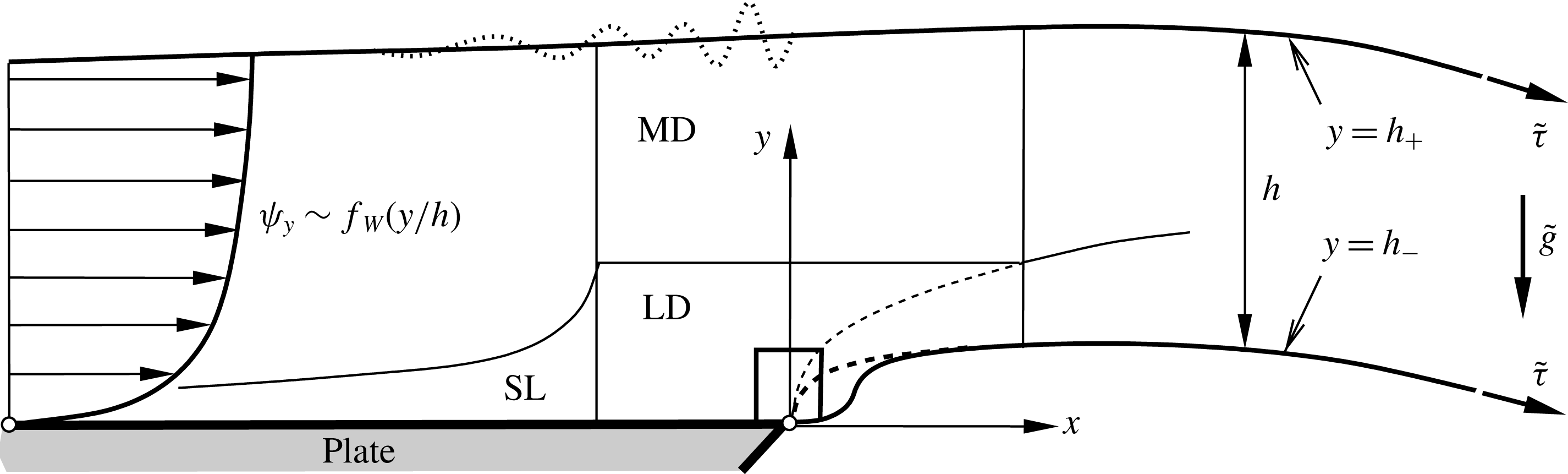
By introducing different flow regions, we will tacitly refer to the sketch in figure 1.
Sketched flow configuration and essential asymptotic regions (not to scale, for definitions see body text); non-interactive/interactive limits (dashed/solid boundaries), tiny NS region (square encompassing plate edge), wavy surface elevation (dotted, see § 4).

3 Non-interactive flow under very weak gravity
We first consider the entire, grossly horizontal layer passing the edge by taking
 $x$
to be of
 $O(1)$
, where we conveniently set
 $z:=y$
(
 $x<0$
) and
 $z:=y-h_{-}(x)$
(a Prandtl transformation for
 $x>0$
). Then the flow exhibits only weak effects due to cross-flow momentum transfer, expressed by the streamline curvature forming the left-hand side of (2.2b
), and the hydrostatic pressure variation, resulting from its right-hand side and (2.2d
). Subscripts indicate unambiguously the respective class of perturbation quantities in the corresponding expansion
 $$\begin{eqnarray}\displaystyle \{\hspace{-1.2pt}[\unicode[STIX]{x1D713},p],[h,h_{\pm }]\hspace{-1.2pt}\} & {\sim} & \displaystyle \{\hspace{-0.6pt}[\bar{\unicode[STIX]{x1D713}},\unicode[STIX]{x1D716}^{2}\bar{p}](x,z),[\bar{h},\bar{h}_{\pm }](x)\hspace{-1.4pt}\}+\unicode[STIX]{x1D716}^{2}\{\hspace{-0.6pt}[\unicode[STIX]{x1D713}_{\unicode[STIX]{x1D716}},\unicode[STIX]{x1D716}^{2}p_{\unicode[STIX]{x1D716}}](x,z),[h_{\unicode[STIX]{x1D716}},h_{\unicode[STIX]{x1D716},\pm }](x)\hspace{-1.3pt}\}\nonumber\\ \displaystyle & & \displaystyle +\,g\{\hspace{-0.7pt}[\unicode[STIX]{x1D713}_{g}(x,z),\bar{h}-z],[h_{g},h_{g,\pm }](x)\hspace{-1.2pt}\}+O(\unicode[STIX]{x1D716}^{3},g\unicode[STIX]{x1D716}^{2},g^{2}).\end{eqnarray}$$
The first of the remainder terms herein is induced by (2.2c,d
). To leading order, (2.2) reduces to a parabolic shallow-water problem that governs the quantities
 $\bar{\unicode[STIX]{x1D713}}$
,
 $\bar{h}$
and describes perfectly supercritical non-uniform flow:
 $$\begin{eqnarray}\displaystyle & \displaystyle \bar{\unicode[STIX]{x1D713}}_{z}^{2}(\bar{\unicode[STIX]{x1D713}}_{x}/\bar{\unicode[STIX]{x1D713}}_{z})_{z}\equiv \bar{\unicode[STIX]{x1D713}}_{z}\bar{\unicode[STIX]{x1D713}}_{zx}-\bar{\unicode[STIX]{x1D713}}_{x}\bar{\unicode[STIX]{x1D713}}_{zz}=\bar{\unicode[STIX]{x1D713}}_{zzz}, & \displaystyle\end{eqnarray}$$
 $$\begin{eqnarray}\displaystyle & \displaystyle z=0:\bar{\unicode[STIX]{x1D713}}=\bar{\unicode[STIX]{x1D713}}_{z}\unicode[STIX]{x1D703}(-x)=\bar{\unicode[STIX]{x1D713}}_{zz}\unicode[STIX]{x1D703}(x)=0,\quad z=\bar{h}(x):\bar{\unicode[STIX]{x1D713}}-1=\bar{\unicode[STIX]{x1D713}}_{zz}=0. & \displaystyle\end{eqnarray}$$
 $+$
and
 $-$
indicate evaluation for
 $y=\bar{h}_{\pm }(x)$
(or, equivalently,
 $z=\bar{h}(x)$
and
 $z=0$
). In turn, (2.2b
) gives in combination with splitting off the hydrostatic pressure introduced by (3.1), (2.2d
) and (3.2) after some manipulations
 $$\begin{eqnarray}\int _{z}^{\bar{h}}\bar{\unicode[STIX]{x1D713}}_{z}^{2}(x,t)\frac{\unicode[STIX]{x2202}}{\unicode[STIX]{x2202}x}\left[\bar{h}_{-}^{\prime }-\frac{\bar{\unicode[STIX]{x1D713}}_{x}(x,t)}{\bar{\unicode[STIX]{x1D713}}_{z}(x,t)}\right]\text{d}t=\bar{\unicode[STIX]{x1D713}}_{zx}+\bar{\unicode[STIX]{x1D713}}_{zx,+}+\unicode[STIX]{x1D70F}\bar{h}_{+}^{\prime \prime }+\bar{p}.\end{eqnarray}$$
In the following, reducing the Froude number from infinity by virtue of the proposition
 $$\begin{eqnarray}\bar{g}:=g/\unicode[STIX]{x1D716}^{2}=O(1)\end{eqnarray}$$
implies a first least-degenerate inclusion of hydrostatic effects. Evaluating (3.3) subject to (3.2b
) and (2.2d
) for
 $z=0$
then yields
 $\bar{p}(x,0)+\bar{g}\bar{h}=\bar{p}_{p}\unicode[STIX]{x1D703}(-x)+(\unicode[STIX]{x1D70F}\bar{h}_{-}^{\prime \prime }-2\bar{\unicode[STIX]{x1D713}}_{zx,-})\unicode[STIX]{x1D703}(x)$
. This determines the leading-order plate pressure denoted by
 $\bar{p}_{p}(x)$
(
 $x\leqslant 0$
) and represents an equation governing
 $\bar{h}_{-}(x)$
(
 $x>0$
).
3.1 Two useful conservation laws
We revisit the variation of streamwise momentum derived from (3.2). Continuity of the flow quantities provides
 $[\bar{\unicode[STIX]{x1D713}}_{0},\bar{h}_{0}]:=[\bar{\unicode[STIX]{x1D713}}(0-,z),\bar{h}(0-)]=[\bar{\unicode[STIX]{x1D713}}(0+,z),\bar{h}(0+)]$
(here and hereafter,
 $0+$
and
 $0-$
indicate one-sided limits in the usual manner) and
 $$\begin{eqnarray}x\leqslant 0:\frac{\text{d}}{\text{d}x}\int _{0}^{\bar{h}}\bar{\unicode[STIX]{x1D713}}_{z}^{2}\,\text{d}z=-\bar{\unicode[STIX]{x1D713}}_{zz,-},\quad x>0:J_{0}:=\int _{0}^{\bar{h}}\bar{\unicode[STIX]{x1D713}}_{z}^{2}\,\text{d}z\equiv \int _{0}^{\bar{h}_{0}}\bar{\unicode[STIX]{x1D713}}_{0}^{\prime 2}\,\text{d}z.\end{eqnarray}$$
Next, we note the two relationships
 $$\begin{eqnarray}\displaystyle \frac{\text{d}}{\text{d}x}\int _{0}^{\bar{h}}\bar{\unicode[STIX]{x1D713}}_{z}^{2}z\,\text{d}z=\bar{\unicode[STIX]{x1D713}}_{z,-}-\bar{\unicode[STIX]{x1D713}}_{z,+}-\int _{0}^{\bar{h}}\bar{\unicode[STIX]{x1D713}}_{z}\bar{\unicode[STIX]{x1D713}}_{x}\,\text{d}z,\quad \frac{\text{d}}{\text{d}x}\int _{0}^{\bar{h}}\bar{\unicode[STIX]{x1D713}}_{z}\bar{\unicode[STIX]{x1D713}}_{x}\,\text{d}z=\int _{0}^{\bar{h}}\bar{\unicode[STIX]{x1D713}}_{z}^{2}\frac{\unicode[STIX]{x2202}}{\unicode[STIX]{x2202}x}\frac{\bar{\unicode[STIX]{x1D713}}_{x}}{\bar{\unicode[STIX]{x1D713}}_{z}}\,\text{d}z & & \displaystyle \nonumber\\ \displaystyle & & \displaystyle\end{eqnarray}$$
obtained by using (3.2b
); the first in addition from multiplying (3.2a
) with
 $z$
and integrating it then from
 $z=0$
to
 $z=\bar{h}$
. We substitute these into the aforementioned differential equation describing
 $\bar{h}_{-}(x)$
derived from (3.3). Using (3.5) and
 $\bar{h}_{-}\bar{\unicode[STIX]{x1D713}}_{zz,-}\equiv 0$
then casts this into the more convenient form expressing the streamwise variation of the angular momentum of the flow around the edge,
 $$\begin{eqnarray}\frac{\text{d}}{\text{d}x}[J_{0}\bar{h}_{-}^{\prime }+K^{\prime }(x)-\unicode[STIX]{x1D70F}\bar{h}_{+}^{\prime }]=\unicode[STIX]{x1D70F}\bar{h}_{-}^{\prime \prime }\unicode[STIX]{x1D703}(x)+\bar{p}_{p}\unicode[STIX]{x1D703}(-x)-\bar{g}\bar{h},\quad K(x):=\int _{0}^{\bar{h}}\bar{\unicode[STIX]{x1D713}}_{z}^{2}z\,\text{d}z.\end{eqnarray}$$
3.2 Perturbed Watson’s self-similar flow
We cast (3.2) in the advantageous form
 $$\begin{eqnarray}\displaystyle & \displaystyle \bar{h}(f_{\unicode[STIX]{x1D702}}f_{\unicode[STIX]{x1D702}x}-f_{x}f_{\unicode[STIX]{x1D702}\unicode[STIX]{x1D702}})-\bar{h}^{\prime }f_{\unicode[STIX]{x1D702}}^{2}=f_{\unicode[STIX]{x1D702}\unicode[STIX]{x1D702}\unicode[STIX]{x1D702}},\quad f(x,\unicode[STIX]{x1D702}):=\bar{\unicode[STIX]{x1D713}}(x,z),\quad \unicode[STIX]{x1D702}:=z/\bar{h}(x), & \displaystyle\end{eqnarray}$$
 $$\begin{eqnarray}\displaystyle & \displaystyle \unicode[STIX]{x1D702}=0:\quad f=f_{\unicode[STIX]{x1D702}}\unicode[STIX]{x1D703}(-x)=f_{\unicode[STIX]{x1D702}\unicode[STIX]{x1D702}}\unicode[STIX]{x1D703}(x)=0,\quad \unicode[STIX]{x1D702}=1:\quad f-1=f_{\unicode[STIX]{x1D702}\unicode[STIX]{x1D702}}=0. & \displaystyle\end{eqnarray}$$
 $x=-1$
, the unique solution to (3.8) for
 $x<0$
is in general found by numerical downstream marching. Subsequently, (3.3) with
 $\bar{h}_{+}=\bar{h}$
determines
 $\bar{p}$
; (3.7) then gives
 $\bar{p}_{p}=\bar{g}\bar{h}+K^{\prime \prime }-\unicode[STIX]{x1D70F}\bar{h}^{\prime \prime }$
. Specifically, the rapid spread of viscous shear across the layer close to its virtual origin
 $x=-1$
,
 $\bar{h}(-1)=0$
indicating jet impingement gives rise to Watson’s self-preserving, i.e. fully developed, flow for
 $x\leqslant 0$
(Watson Reference Watson1964; Bowles & Smith Reference Bowles and Smith1992; Higuera Reference Higuera1994; Scheichl & Kluwick Reference Scheichl and Kluwick2017):
 $[f,\bar{h}]=[f_{W}(\unicode[STIX]{x1D702}),h_{W}(x)]$
,
 $h_{W}(x):=a_{W}(x+1)$
,
 $a_{W}:=\unicode[STIX]{x03C0}/\sqrt{3}\simeq 1.8138$
. By (3.8),
 $$\begin{eqnarray}-a_{W}f_{W}^{\prime 2}=f_{W}^{\prime \prime \prime },\quad f_{W}(0)=f_{W}^{\prime }(0)=f_{W}^{\prime \prime }(1)=0,\quad f_{W}(1)=1,\end{eqnarray}$$
yields
 $f_{W}$
,
 $a_{W}$
in closed form (cf. Scheichl & Kluwick Reference Scheichl and Kluwick2017). Other key results are
 $f_{W}^{\prime }(1)=[\unicode[STIX]{x0393}(1/3)/\unicode[STIX]{x0393}(5/6)]^{2}/(2\sqrt{3})\simeq 1.6260$
,
 $\unicode[STIX]{x1D706}_{W}:=f_{W}^{\prime \prime }(0)=\sqrt{2a_{W}/3}~f_{W}^{\prime 3/2}(1)\simeq 2.2799$
and
 $$\begin{eqnarray}J_{0}=\unicode[STIX]{x1D706}:=\frac{\unicode[STIX]{x1D706}_{W}}{a_{W}^{2}}\simeq 0.6930,\quad K\equiv K_{W}:=\frac{f_{W}^{\prime }(1)}{a_{W}}\simeq 0.8964,\quad \bar{p}=p_{W}:=\frac{2a_{W}f_{W}^{\prime }(\unicode[STIX]{x1D702})}{h_{W}^{2}(x)}.\end{eqnarray}$$
Most importantly,
 $\unicode[STIX]{x1D706}$
represents the shear rate exerted at the plate edge. We hence obtain
 $\bar{p}_{p}=\bar{g}h_{W}$
with no capillary influence due to the linear increase in
 $h_{W}(x)$
. If not stated otherwise, we refer to the above values and definitions tacitly below.
3.2.1 Regular perturbations
Hereafter, we confidently ignore any disturbances of the fully developed flow resorting to jet impact as these do not affect the subsequent analysis crucially. As a consequence, potential eigensolutions of the linearised operator in (3.8) can be safely ignored. This justifies the form of the expansion (3.1) for regular perturbations, varying in the streamwise direction only with
 $x$
, i.e. on the global scale, in the limits considered.
As seen from (2.2a
), those deviations of the shallow-water limit then arise by the pressure and normal-stress gradients in terms of the inhomogeneities
 $-\unicode[STIX]{x1D716}^{2}\bar{h}^{3}(\bar{p}_{x}-\bar{\unicode[STIX]{x1D713}}_{zxx})$
and
 $-\unicode[STIX]{x1D716}^{2}\bar{g}\bar{h}^{3}\bar{h}^{\prime }$
added to the right-hand side of the expanded form of (3.8a
). In turn,
 $h_{\unicode[STIX]{x1D716},g}$
are found by virtue of the linearised kinematic BCs (2.2c
) and free-slip condition in (2.2d
)
 $$\begin{eqnarray}\displaystyle & \displaystyle [\unicode[STIX]{x1D713}_{\unicode[STIX]{x1D716},g},\unicode[STIX]{x2202}_{z}\unicode[STIX]{x1D713}_{\unicode[STIX]{x1D716},g}](x,0)=[0,0],\quad \unicode[STIX]{x1D713}_{\unicode[STIX]{x1D716},g}(x,\bar{h})=-h_{\unicode[STIX]{x1D716},g}\bar{\unicode[STIX]{x1D713}}_{z}(x,\bar{h}), & \displaystyle\end{eqnarray}$$
 $$\begin{eqnarray}\displaystyle & \displaystyle z=\bar{h}:[\unicode[STIX]{x1D713}_{\unicode[STIX]{x1D716}},\unicode[STIX]{x1D713}_{g}]_{zz}=-h_{\unicode[STIX]{x1D716},g}\bar{\unicode[STIX]{x1D713}}_{zzz}[1,1]+[\bar{\unicode[STIX]{x1D713}}_{xx}+2\bar{h}^{\prime }\bar{\unicode[STIX]{x1D713}}_{zx},0]. & \displaystyle\end{eqnarray}$$
We first consider those essentially accounting for momentum transfer and normal stresses in the vertical direction. The representations of
 $\bar{\unicode[STIX]{x1D713}}$
in (3.9) and
 $\bar{p}$
in (3.10) and (3.8) suggest we write
 $[\unicode[STIX]{x1D713}_{\unicode[STIX]{x1D716}},h_{\unicode[STIX]{x1D716}}/h_{W}]=[f_{\unicode[STIX]{x1D716}}(\unicode[STIX]{x1D702}),H_{\unicode[STIX]{x1D716}}]$
with the latter quantities determined by the boundary-value problem
 $$\begin{eqnarray}\displaystyle 2a_{W}f_{W}^{\prime }f_{\unicode[STIX]{x1D716}}^{\prime }+f_{\unicode[STIX]{x1D716}}^{\prime \prime \prime }=-(\unicode[STIX]{x1D702}^{3}f_{W}^{\prime })^{\prime \prime }/\unicode[STIX]{x1D702},\quad f_{\unicode[STIX]{x1D716}}(0)=f_{\unicode[STIX]{x1D716}}^{\prime }(0)=0,\quad (f_{\unicode[STIX]{x1D716}}^{\prime \prime }/f_{\unicode[STIX]{x1D716}})(1)=(f_{W}^{\prime \prime \prime }/f_{W}^{\prime })(1) & & \displaystyle \nonumber\\ \displaystyle & & \displaystyle\end{eqnarray}$$
and
 $H_{\unicode[STIX]{x1D716}}=-(f_{\unicode[STIX]{x1D716}}/f_{W}^{\prime })(1)$
. Here the expressions of the inhomogeneities ensue after some lengthy rearrangements; the second contribution to
 $f_{\unicode[STIX]{x1D716}}^{\prime \prime }(1)$
as given by (3.11) is found to vanish. Standard methods allow for an analytical albeit (due to the inhomogeneous BCs) implicit representation of the unique solution to (3.12). We therefore solved (3.12) numerically in a straightforward fashion. With
 $f_{\unicode[STIX]{x1D716}}\geqslant 0$
(figure 2
a), those perturbations are of an expansive (accelerating) nature: they increase the wall shear stress (
 $f_{\unicode[STIX]{x1D716}}^{\prime \prime }(0)\simeq 15.0837$
) and decrease the film height accordingly (
 $H_{\unicode[STIX]{x1D716}}\simeq -3.0338$
).
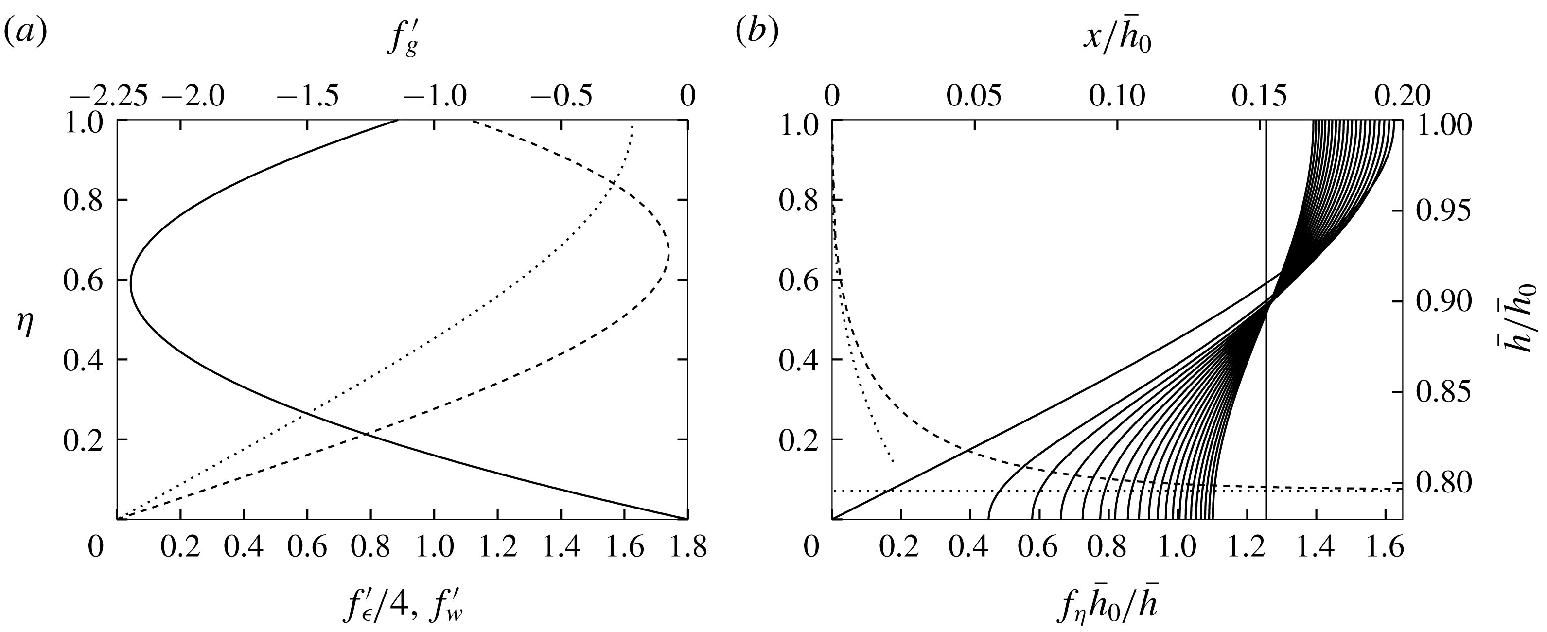
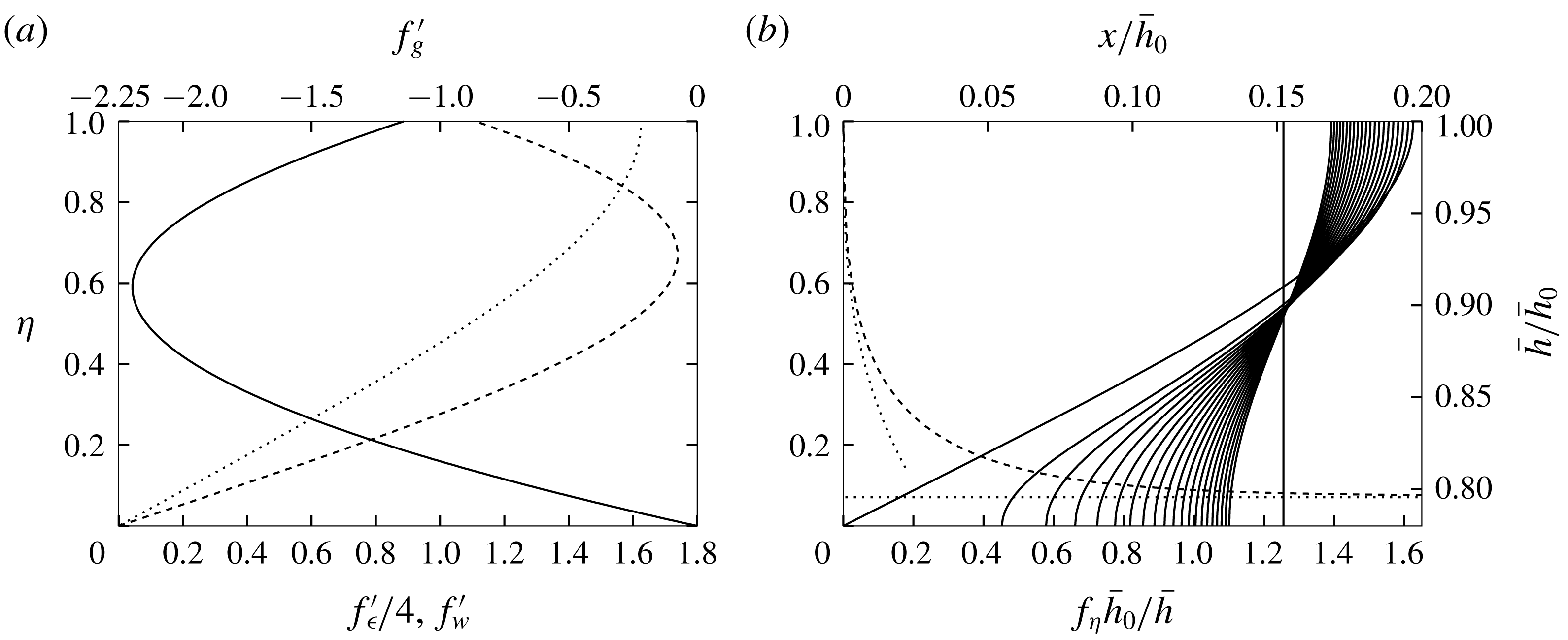
(a) Shape functions
 $f_{\unicode[STIX]{x1D716}}^{\prime }(\unicode[STIX]{x1D702})/4$
(dashed),
 $f_{g}^{\prime }(\unicode[STIX]{x1D702})$
(solid) referring to cross-stream and hydrostatic perturbations of Watson’s flow profile
 $f_{W}^{\prime }(\unicode[STIX]{x1D702})$
(dotted); (b) detached flow, normalised by
 $\bar{h}_{0}$
: flow profiles
 $f_{\unicode[STIX]{x1D702}}\bar{h}_{0}/\bar{h}$
(solid) versus
 $\unicode[STIX]{x1D702}$
for
 $x=0$
(Watson’s profile),
 $x/\bar{h}_{0}=0.005i$
(
 $i=1,2,\ldots ,20$
),
 $x/\bar{h}_{0}=0.999$
, note
 $f_{\unicode[STIX]{x1D702}x}(x,0)>0$
, and
 $\bar{h}/\bar{h}_{0}$
versus
 $x/\bar{h}_{0}$
(dashed), asymptotes of
 $\bar{h}/\bar{h}_{0}$
for
 $x\rightarrow 0$
,
 $x\rightarrow \infty$
considered in §§ 3.3.3, 3.3.2 (dotted).
The subsequently more relevant hydrostatically induced regular disturbances (§ 4.1) add the term
 $-ga_{W}h_{W}^{3}$
to the right-hand side of the correspondingly linearised version of (3.8a
). We in turn arrive at
 $[\unicode[STIX]{x1D713}_{g},h_{g}/h_{W}]=(1+x)^{3}[f_{g}(\unicode[STIX]{x1D702}),H_{g}]$
and conveniently set
 $f_{g}=f_{W}^{\prime }G_{g}$
. With the aid of (3.9) and (3.11),
 $G_{g}$
and
 $H_{g}$
then satisfy
 $$\begin{eqnarray}4a_{W}f_{W}^{\prime 4}G_{g}^{\prime }=(f_{W}^{\prime 3}G_{g}^{\prime \prime })^{\prime }-a_{W}^{4}f_{W}^{\prime 2},\quad G_{g}(0)=G_{g}^{\prime \prime }(1)=0,\quad H_{g}=-G_{g}(1).\end{eqnarray}$$
The regularity condition
 $G_{g}^{\prime \prime }(0)=a_{W}^{4}/(3\unicode[STIX]{x1D706}_{W})$
completes (3.13) to form a boundary-value problem. A numerical investigation shows that the associated self-adjoint homogeneous problem has no solution (and thus the absence of the aforementioned eigensolutions or free perturbations for the specific streamwise variation considered). Hence, (3.13) uniquely determines
 $G_{g}^{\prime }$
and
 $G_{g}$
,
 $H_{g}$
by subsequent integration. Here the straightforward numerical solution of (3.13) predicts
 $f_{g}\leqslant 0$
(figure 2
a),
 $f_{g}^{\prime \prime }(0)=2\unicode[STIX]{x1D706}_{W}[G_{g}^{\prime }(0)+H_{g}]\simeq -2.6272$
and
 $H_{g}\simeq 0.9907$
. Contrasting sharply with the irregular short-scale perturbations studied below and in § 4.1, the adverse hydrostatic pressure gradient first yields a weakly compressive (retarded) flow.
3.2.2 Irregular perturbations
Bowles & Smith (Reference Bowles and Smith1992) showed how weak perturbations of rapid downstream growth can exist in very supercritical developed shallow-water flow so as to provoke an accordingly strong hydraulic jump via local free viscous–inviscid interaction of double-layer type. For finite values of
 $x+1$
, that interaction process would occur along a horizontal length of
 $O(g^{3})$
in the current specification of the flow. The similar scenario for disturbances due to cross-stream effects yields an interaction length of
 $\unicode[STIX]{x1D716}^{6/7}$
as derived originally by Smith (Reference Smith1977) and Smith & Duck (Reference Smith and Duck1977). Raising the magnitude of
 $g$
to
 $O(\unicode[STIX]{x1D716}^{2/7})$
establishes the distinguished limit Bowles & Smith (Reference Bowles and Smith1992) considered. Complying with Higuera’s (Reference Higuera1994) analysis, however, here the presumed existence of the trailing edge, so introducing the basic streamwise scale, avoids that jump in the limit
 $g\rightarrow 0$
to keep the flow correspondingly close to supercritical conditions. Hence, the present embedding keeps the magnitude of those rapidly growing perturbations from attaining a magnitude that triggers that strong interaction sufficiently far upstream from the plate edge. On the other hand, Brotherthon-Ratcliffe & Smith (Reference Brotherton-Ratcliffe and Smith1989) identified a type of Korteweg–de-Vries wave interacting with a Stokes layer that perturbs a developed layer described by the hydrostatic extension of the shallow-water approximation, with the basic phase speed given by the unperturbed flow, on a relatively large longitudinal scale measured by
 $\unicode[STIX]{x1D716}^{-1/5}$
, and slowly modulated on an associated time scale measured by
 $\unicode[STIX]{x1D716}^{-3/5}$
. Following their analysis (also Balmforth Reference Balmforth1999), the so-manifested upstream influence and possible destabilisation of the hydrostatic extension of the shallow-water approximation vanish only for
 $g=0$
: this then precisely coins the notion of supercritical developed flow.
Both contexts suggest the existence of longitudinal short-scale disturbances in the present situation. We study these in the necessary breadth and depth as their strengths and variations through the flow are found to both complete the parametrisation of the strongly interactive near-edge flow in § 4.1 and to identify the full extent of the upstream influence.
The effects of gravity and of streamline curvature including the capillary influence generate a family of perturbations characterised by locally rapid variation but of exponentially small amplitude. These promote further contributions to (3.1) for
 $\unicode[STIX]{x1D716}\rightarrow 0$
and
 $g\rightarrow 0$
where the distinguished limit (3.4) can be relaxed. Due to the scale reduction, they represent homogeneous disturbances about the shallow-water limit above their generating viscous near-plate region where
 $N:=\unicode[STIX]{x1D702}/\unicode[STIX]{x1D6E5}=O(1)$
, say; the asymptotically small gauge function
 $\unicode[STIX]{x1D6E5}(\unicode[STIX]{x1D716};x)$
is positive downstream of the virtual origin (for
 $x>-1$
). Since a nonlinear distortion of the unperturbed shear flow in this viscous sublayer (SL), represented by
 $f_{W}^{\prime }\sim \unicode[STIX]{x1D706}_{W}\unicode[STIX]{x1D702}$
, would typically require
 $1+x=O(\unicode[STIX]{x1D6E5}^{1/3})$
along the plate, it is ruled out. This renders a linearisation of (2.2) across the entire layer sufficient. The viscous displacement of the streamlines in the SL provokes likewise rapid disturbances in the core layer, hence satisfying the inviscid-flow equations to leading order. For larger values of
 $\bar{g}$
, the purely hydrostatically caused disturbances were first shown by Bowles (Reference Bowles1990) to originate from the singular point
 $x=-1$
, associated with their exponentially fast streamwise growth; cf. Scheichl & Bowles (Reference Scheichl and Bowles2017) and Scheichl & Kluwick (Reference Scheichl and Kluwick2017). Here we revise and extend this analysis of the associated singularly perturbed eigenproblems.
It is useful at this stage to first demonstrate why the thereby introduced shortest streamwise scales are, however, sufficiently long to avoid the formation of a Rayleigh stage and thus a corresponding finite streamwise slip at its base. Its inevitable breakdown close to the latter would either be of inviscid and nonlinear character or directly controlled by viscous shear. Together with the no-slip condition holding at the plate, the first type would yield a further viscous slip flow adjacent to it, driven by an imposed pressure gradient. However, this impedes a strong interaction mechanism (of the above kind) required to control the flow around the edge as outlined further below. The second would imply an (interactive) two-tiered structure, crucially tied in with the displacement effect mentioned before. But in conflict with the assumption of a Rayleigh limit, then the pressure disturbances in the core tier are typically controlled by their cross-stream variation (meaning a hierarchical slender-layer approximation).
We bear these arguments in mind when it comes to the rationale underlying the interactive-flow structure. In the present context of linearising (2.2a,b
) for
 $\unicode[STIX]{x1D702}=O(1)$
, they justify us taking the irregular pressure perturbations balancing streamline curvature (and the gradients of the normal stresses), see (2.2b
), as insignificantly small in the expanded form of (2.2a
). By the smallness of
 $g$
, this also holds for their hydrostatically induced counterparts. We then linearise (2.2) by ignoring the BCs for
 $y=0$
and noting
 $p_{W}(x,\unicode[STIX]{x1D702})$
as given by (3.10). This yields
 $\unicode[STIX]{x1D713}\sim f_{W}$
perturbed by the aforesaid local eigenfunction at negligibly small pressure disturbances ensuing from (2.2b
) and the last of the BCs (2.2d
) with the aid of (3.1) (subject to
 $\unicode[STIX]{x2202}_{\unicode[STIX]{x1D702}}p_{W}(x,1)=0$
):
 $$\begin{eqnarray}\displaystyle \displaystyle [\unicode[STIX]{x1D713},h/h_{W}(x)] & {\sim} & \displaystyle [f_{W}(\unicode[STIX]{x1D702}),1]+\cdots +\unicode[STIX]{x1D6FE}(\unicode[STIX]{x1D716};x)[f_{W}^{\prime }(\unicode[STIX]{x1D702}),-1]+\text{c.c.}+o(\unicode[STIX]{x1D6FE}),\end{eqnarray}$$
 $$\begin{eqnarray}\displaystyle \displaystyle p/\unicode[STIX]{x1D716}^{2} & {\sim} & \displaystyle p_{W}(x,\unicode[STIX]{x1D702})+\cdots +\unicode[STIX]{x1D6FE}_{xx}P_{\unicode[STIX]{x1D716}}(x,\unicode[STIX]{x1D702})-\unicode[STIX]{x1D6FE}\bar{g}h_{W}(x)+\text{c.c.}+o(\unicode[STIX]{x1D6FE}_{xx},\unicode[STIX]{x1D6FE}\bar{g}),\qquad \quad\end{eqnarray}$$
 $$\begin{eqnarray}\displaystyle & \displaystyle P_{\unicode[STIX]{x1D716}}(x,\unicode[STIX]{x1D702}):=\unicode[STIX]{x1D70F}h_{W}(x)-\int _{\unicode[STIX]{x1D702}}^{1}f_{W}^{\prime 2}(t)\,\text{d}t=\unicode[STIX]{x1D70F}h_{W}-\frac{f_{W}^{\prime \prime }}{a_{W}}.\qquad \quad & \displaystyle\end{eqnarray}$$
 $\unicode[STIX]{x1D6FE}$
of fast variation in
 $x$
is supposed to vanish as
 $\unicode[STIX]{x1D716}\rightarrow 0$
, and the dots indicate the higher-order regular terms already absorbed by (3.1). Specifically, we have not only anticipated
 $\unicode[STIX]{x1D6FE}=o(\unicode[STIX]{x1D6FE}_{x})$
, implying
 $\unicode[STIX]{x1D6FE}_{x}=o(\unicode[STIX]{x1D6FE}_{xx})$
and
 $\unicode[STIX]{x1D6FE}_{xx}=o(\unicode[STIX]{x1D6FE}_{xxx})$
, but also
 $$\begin{eqnarray}\unicode[STIX]{x1D716}^{2}\unicode[STIX]{x1D6FE}_{xxx}=o(\unicode[STIX]{x1D6FE}_{xx}).\end{eqnarray}$$
This prompts us to disregard the viscous stresses when expanding (2.2b,d
) and express
 $P_{\unicode[STIX]{x1D716}}$
in (3.14c
) through streamline curvature solely, with the help of (3.9).
From (3.14a
)–(3.15), we deduce the following estimates holding in the SL: with
 $p_{W}(x,0)\equiv 0$
by (3.10), irregular disturbances of
 $O(\unicode[STIX]{x1D6FE}_{xx})$
contribute to the accordingly reduced pressure
 $p/\unicode[STIX]{x1D716}^{2}+(\unicode[STIX]{x1D6FE}-1)\bar{g}h_{W}(x)$
; therefore, the magnitudes of its
 $x$
- and
 $y$
-gradients (of
 $O(\unicode[STIX]{x1D6FE}_{xxx})$
and
 $O(\unicode[STIX]{x1D6FE}_{xx}/\unicode[STIX]{x1D6E5})$
respectively) are much larger than those of the respective perturbations of the normal-stress gradients in (2.2a
) and (2.2b
) (of
 $O(\unicode[STIX]{x1D6FE}_{xx})$
and
 $O(\unicode[STIX]{x1D716}^{2}\unicode[STIX]{x1D6E5}\unicode[STIX]{x1D6FE}_{xxx})$
respectively). Hence, for
 $N=O(1)$
we expand
 $$\begin{eqnarray}\displaystyle & \displaystyle \unicode[STIX]{x1D713}-\unicode[STIX]{x1D706}_{W}\unicode[STIX]{x1D702}^{2}/2\sim \cdots +\unicode[STIX]{x1D6E5}\unicode[STIX]{x1D6FE}\unicode[STIX]{x1D706}_{W}F(N)+\text{c.c.}+o(\unicode[STIX]{x1D6E5}\unicode[STIX]{x1D6FE}), & \displaystyle\end{eqnarray}$$
 $$\begin{eqnarray}\displaystyle & \displaystyle p/\unicode[STIX]{x1D716}^{2}+(\unicode[STIX]{x1D6FE}-1)\bar{g}h_{W}(x)\sim \cdots +\unicode[STIX]{x1D6FE}_{xx}P_{p}(x)+\text{c.c.}+o(\unicode[STIX]{x1D6E5}^{2}\unicode[STIX]{x1D6FE}_{xx},\unicode[STIX]{x1D6FE}\bar{g}), & \displaystyle\end{eqnarray}$$
 $$\begin{eqnarray}\displaystyle & \displaystyle P_{p}(x):=P_{\unicode[STIX]{x1D716}}(x,0)=a_{W}\unicode[STIX]{x1D706}[T(x+1)-1],\quad T:=\unicode[STIX]{x1D70F}/J_{0}, & \displaystyle\end{eqnarray}$$
 $T$
parametrising the pressure disturbances at the plate,
 $P_{p}$
, measures the capillary force relative to the horizontal momentum; here specified by the first relationship in (3.10). We aim to determine
 $\unicode[STIX]{x1D6E5}$
,
 $\unicode[STIX]{x1D6FE}$
and the shape function
 $F$
. Upon substitution into (2.2a
), this yields with the aid of (3.8a
) the least-degenerate balance
 $$\begin{eqnarray}\unicode[STIX]{x1D706}_{W}^{2}h_{W}\unicode[STIX]{x1D6E5}^{3}\unicode[STIX]{x1D6FE}_{x}(NF^{\prime }-F)\sim h_{W}^{3}(\unicode[STIX]{x1D716}\unicode[STIX]{x1D6E5})^{2}[\unicode[STIX]{x1D6FE}_{x}\bar{g}h_{W}-\unicode[STIX]{x1D6FE}_{xxx}P_{p}(x)]+\unicode[STIX]{x1D706}_{W}\unicode[STIX]{x1D6FE}F^{\prime \prime \prime }.\end{eqnarray}$$
One finds
 $\unicode[STIX]{x1D6FE}$
varying much more rapidly with
 $x$
than
 $\unicode[STIX]{x1D6E5}$
. Differentiation of (3.17) with respect to
 $N$
suggests to write
 $\unicode[STIX]{x1D70E}NF^{\prime \prime }=F^{(4)}$
subject to
 $F(0)=F^{\prime }(0)=0$
and
 $F^{\prime }(\infty )=1$
and with the (over
 $x$
piecewise) constant
 $\unicode[STIX]{x1D70E}:=\unicode[STIX]{x1D706}_{W}h_{W}\lim _{\unicode[STIX]{x1D716}\rightarrow 0}(\unicode[STIX]{x1D6E5}^{3}\unicode[STIX]{x1D6FE}_{x}/\unicode[STIX]{x1D6FE})$
by consistency with (3.17). In turn,
 $$\begin{eqnarray}F(N)=3\unicode[STIX]{x1D70E}^{1/3}\int _{0}^{N}(N-t)\text{Ai}(\unicode[STIX]{x1D70E}^{1/3}t)\,\text{d}t,\quad \frac{\unicode[STIX]{x1D6FE}}{\unicode[STIX]{x1D6FE}_{0}(\unicode[STIX]{x1D716})}\sim \exp \int _{0}^{x}\frac{\unicode[STIX]{x1D70E}+o(h_{W}\unicode[STIX]{x1D6E5}^{3})}{\unicode[STIX]{x1D706}_{W}h_{W}(s)\unicode[STIX]{x1D6E5}^{3}(\unicode[STIX]{x1D716};s)}\,\text{d}s\end{eqnarray}$$
for
 $-1<x<0$
and
 $-\unicode[STIX]{x03C0}<\arg \unicode[STIX]{x1D70E}<\unicode[STIX]{x03C0}$
. As
 $\unicode[STIX]{x1D6E5}/\unicode[STIX]{x1D70E}^{1/3}$
proves invariant against a variation in the definition of
 $\unicode[STIX]{x1D6E5}$
, this is seen to absorb any potential
 $x$
-dependence of
 $\unicode[STIX]{x1D70E}$
and thus of
 $F$
. We then preferably choose
 $|\unicode[STIX]{x1D70E}|=1$
, thus
 $$\begin{eqnarray}\unicode[STIX]{x1D70E}=1\end{eqnarray}$$
as long as the streamwise variation of
 $\unicode[STIX]{x1D6FE}$
stays real, and are aware that a potential sudden emergence of a non-zero
 $\arg \unicode[STIX]{x1D70E}$
is tied in with a corresponding shortening of the streamwise scale, then requiring a proper smoothing. The, at first arbitrary, (complex) quantity
 $\unicode[STIX]{x1D6FE}_{0}$
in (3.18) parametrises the strength of the irregular disturbances once they have evolved towards a terminal state asymptotically close to the edge. The herewith introduced upstream influence not only accounts for the singularity of the integrand in (3.18) at the virtual origin but will become fixed in § 4.1. In combination with (3.18), the premise
 $\unicode[STIX]{x1D6FE}=o(\unicode[STIX]{x1D6E5})$
made implicitly in (3.14a
) yields
 $(\unicode[STIX]{x1D6E5}^{3})_{x}=o(h_{W}^{-1})$
, which will turn out to hold even for
 $x\rightarrow -1$
.
Consistency with (3.17) also requires, after some algebra and with the help of (3.16c ),
 $$\begin{eqnarray}\displaystyle & \displaystyle I^{7}-G_{\unicode[STIX]{x1D716}}(1+x)^{3}I^{6}=1-T(1+x), & \displaystyle\end{eqnarray}$$
 $$\begin{eqnarray}\displaystyle & \displaystyle I:=\frac{3^{2/21}\unicode[STIX]{x1D706}^{3/7}a_{W}}{\unicode[STIX]{x0393}(1/3)^{1/7}}\frac{\unicode[STIX]{x1D6E5}}{\unicode[STIX]{x1D70E}^{1/3}\unicode[STIX]{x1D716}^{2/7}},\quad G_{\unicode[STIX]{x1D716}}:=\frac{\unicode[STIX]{x0393}(1/3)^{6/7}}{3^{4/7}\unicode[STIX]{x1D706}^{11/7}}\frac{g}{\unicode[STIX]{x1D716}^{2/7}}. & \displaystyle\end{eqnarray}$$
 $\unicode[STIX]{x1D6FE}_{xxx}/\unicode[STIX]{x1D6FE}\sim (\unicode[STIX]{x1D6FE}_{x}/\unicode[STIX]{x1D6FE})^{3}$
as represented via (3.18), and (3.20b
) from (3.10). Solving (3.20a
) for
 $I$
finally determines
 $\unicode[STIX]{x1D6E5}/\unicode[STIX]{x1D70E}^{1/3}$
and its dependence on the parameters
 $G_{\unicode[STIX]{x1D716}}$
and
 $T$
. It elucidates the necessity of treating both associated effects in a combined fashion; a positive value of
 $G_{\unicode[STIX]{x1D716}}$
introduces a new distinguished limit
 $g=O(\unicode[STIX]{x1D716}^{2/7})$
. The results for the limiting case of dominant gravitational effects,
 $G_{\unicode[STIX]{x1D716}}\gg 1$
giving
 $I\sim (1+x)^{3}G_{\unicode[STIX]{x1D716}}$
and (3.19), match those in the previously mentioned studies by Bowles (Reference Bowles1990), Scheichl & Bowles (Reference Scheichl and Bowles2017) where
 $g=O(1)$
for
 $x$
being sufficiently close to
 $-1$
. However, the restoring impact of streamline curvature on (3.20a
) is revealed by the distinguished limit
 $I-I^{-6}\sim G_{\unicode[STIX]{x1D716}}(1+x)^{3}=O(1)$
, serving to rectify that analysis. By assuming moderately large values of
 $G_{\unicode[STIX]{x1D716}}$
, we deduce
 $\unicode[STIX]{x1D6E5}=O(\unicode[STIX]{x1D716}^{2/7})$
for
 $-1\leqslant x<0$
so that (3.15) is satisfied and our current analysis stays intact in the limit
 $x\rightarrow -1$
. Since
 $\text{Re}(\unicode[STIX]{x1D70E}^{1/3})>0$
, only roots having
 $\text{Re}\,I>0$
are admitted. Furthermore, perturbations growing in the downstream direction require
 $\text{Re}\,\unicode[STIX]{x1D70E}>0$
according to (3.18), which implies
 $I\rightarrow 1$
as
 $x\rightarrow -1$
.
For the large Froude numbers considered here, consistency with § 4, below, which takes
 $g=O(\unicode[STIX]{x1D716}^{4/7})$
, requires us to concentrate here on the case
 $G_{\unicode[STIX]{x1D716}}=0$
, i.e. to neglect the gravitational influence in (3.20a
). We include it, however, for completeness and for consideration in our subsequent work examining smaller values of the Froude number, as outlined in § 5. Some of the impact of finite but small values of
 $G_{\unicode[STIX]{x1D716}}$
is taken up in appendix A.
For the current negligibly small values of
 $G_{\unicode[STIX]{x1D716}}$
and also
 $T$
, then
 $I\sim 1$
throughout and (3.18) signifies a strong algebraic downstream growth, which close to the plate edge is transformed into an exponential one:
 $$\begin{eqnarray}\displaystyle & \displaystyle \unicode[STIX]{x1D6FE}/\unicode[STIX]{x1D6FE}_{0}\underset{x=O(1)}{{\sim}}(1+x)^{E}\underset{x\rightarrow 0-}{{\sim}}\exp (Ex),\quad E:=(B\unicode[STIX]{x1D716})^{-6/7}\rightarrow \infty , & \displaystyle\end{eqnarray}$$
 $$\begin{eqnarray}\displaystyle & \displaystyle B:=\frac{\unicode[STIX]{x0393}(1/3)^{3/7}}{(3\unicode[STIX]{x1D706})^{2/7}}=\left(\frac{4\unicode[STIX]{x03C0}^{3}\unicode[STIX]{x0393}(5/6)^{6}}{3\unicode[STIX]{x0393}(1/3)^{3}}\right)^{1/7}\simeq 1.2376, & \displaystyle\end{eqnarray}$$
 $G_{\unicode[STIX]{x1D716}}$
and
 $T$
are not both vanishingly small, the perturbations grow exponentially for increasing values of
 $x$
, according to (3.18). Such an exponential growth is also expected for the precursors of these disturbances in the regions closer to jet impact where the flow is not fully developed, i.e.
 $h$
not increasing linearly with
 $x$
in the shallow-water limit. Correspondingly, the first of the relationships (3.21) describes a required matching law in the limit
 $x+1\rightarrow 0+$
, from which we infer that the perturbations can indeed only exist along the entire plate if
 $\text{Re}\,\unicode[STIX]{x1D70E}>0$
, and the second relation in (3.21a
) represents a special case of the behaviour
 $$\begin{eqnarray}\unicode[STIX]{x1D6FE}/\unicode[STIX]{x1D6FE}_{0}\sim \exp [Ex/I_{0}^{3}+o(x)],\quad x/\unicode[STIX]{x1D716}^{6/7}\rightarrow 0-.\end{eqnarray}$$
Herein,
 $I_{0}$
denotes a permitted root of (3.20a
) for
 $x=0$
. The exponentially growing amplitude of the perturbations has attained its final order of magnitude for
 $x=O(\unicode[STIX]{x1D716}^{6/7})$
upstream of the plate edge.
As a result, we first trace a single branch of positive roots of (3.20a
) in the downstream direction, starting with
 $I=1$
, along with the setting (3.19). For
 $T<1$
, all involved perturbation quantities stay real up to the plate edge. If
 $T>1$
, however, we encounter a sudden modification of the shape function
 $F$
in (3.18) (on the original streamwise
 $O(1)$
-scale) as
 $$\begin{eqnarray}\unicode[STIX]{x1D70E}=\exp (-3\text{i}\unicode[STIX]{x03C0}/7),\quad x_{T}:=1/T-1<x<0.\end{eqnarray}$$
Here
 $x=x_{T}$
indicates a so-called ‘capillary threshold’ where
 $P_{p}(x)$
in (3.16c
) changes sign as its capillary portion overcompensates that by vertical momentum transfer for
 $x>x_{T}$
. With the aid of (3.20a
) and (3.22), we finally track the logarithmic attenuation
 $\unicode[STIX]{x1D6FE}/\unicode[STIX]{x1D6FE}_{0}$
of the capillarity-controlled disturbances from the edge in upstream direction in the form
 $$\begin{eqnarray}B\unicode[STIX]{x1D716}^{6/7}\ln \left(\frac{\unicode[STIX]{x1D6FE}}{\unicode[STIX]{x1D6FE}_{0}}\right)\sim \unicode[STIX]{x1D6FA}(x;T):=\int _{0}^{x}\frac{\text{d}s}{(1+s)[1-T(1+s)]^{3/7}},\quad I_{0}=\frac{1}{(1-T)^{1/7}},\end{eqnarray}$$
where we note (3.21) arising in the limit
 $T\rightarrow 0$
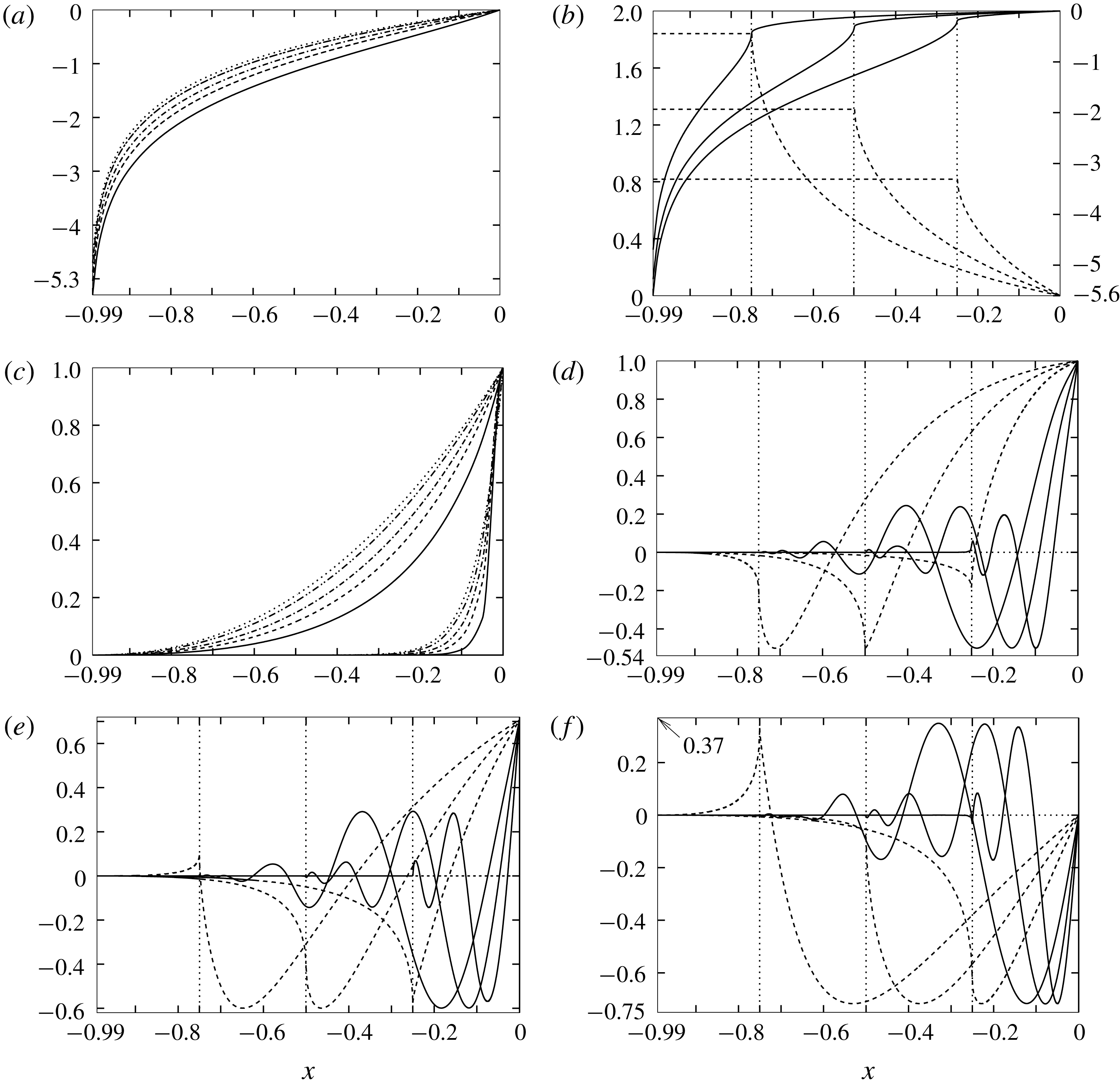
. Figure 3 illustrates the numerical evaluation of the scaled exponent
 $\unicode[STIX]{x1D6FA}$
in (3.18): one clearly identifies the logarithmic singularity of
 $\unicode[STIX]{x1D6FA}$
and the associated algebraic one of
 $\unicode[STIX]{x1D6FE}/\unicode[STIX]{x1D6FE}_{0}$
at
 $x=-1$
, included in (3.21); its integrable counterpart of
 $\unicode[STIX]{x1D6FA}$
at
 $x=x_{T}$
, accompanying the abrupt switch from (3.19) to (3.23) in the case
 $T>1$
; the exponential steepening of
 $\unicode[STIX]{x1D6FE}/\unicode[STIX]{x1D6FE}_{0}$
upstream of the plate edge, the more extreme the smaller
 $\unicode[STIX]{x1D716}$
is. Most important, for
 $T>1$
we find
 $\arg I=\unicode[STIX]{x03C0}/7$
(0) for
 $x>x_{T}$
(
 $x<x_{T}$
) such that
 $\text{Im}\,\unicode[STIX]{x1D6FA}$
increases from zero for
 $x=0$
in the upstream direction towards its final value assumed for
 $x\leqslant x_{T}$
, where
 $\arg \unicode[STIX]{x1D6FE}=\arg \unicode[STIX]{x1D6FE}_{0}+\arg \unicode[STIX]{x1D6FA}$
. This expresses a subtle cumulative upstream influence. As a physically intriguing phenomenon, stationary capillarity-driven undulations of the flow originate from the capillary threshold to grow exponentially towards the plate edge. Both their frequency and the slope of their envelope increase for decreasing values of
 $\unicode[STIX]{x1D716}$
. For figure 3(c–d), we have used
 $\unicode[STIX]{x1D6FE}/|\unicode[STIX]{x1D6FE}_{0}|\sim \exp [\unicode[STIX]{x1D6FA}/(B\unicode[STIX]{x1D716}^{6/7})+\text{i}\arg \unicode[STIX]{x1D6FE}_{0}]$
. Hence, considering just the real part by varying
 $\arg \unicode[STIX]{x1D6FE}$
from 0 to
 $\unicode[STIX]{x03C0}$
surveys the potential variety of the streamwise oscillations.
 $\unicode[STIX]{x1D6FA}$
and
 $\unicode[STIX]{x1D6FE}/\unicode[STIX]{x1D6FE}_{0}$
versus
 $x$
given by (3.24) (cubic-spline interpolation of computed data points); (a)
 $\unicode[STIX]{x1D6FA}$
for
 $T=0$
(dotted), 0.2 (dot-dot-dashed), 0.5 (dot-dashed), 0.7 (dashed), 0.9 (solid); (b)
 $\text{Re}\,\unicode[STIX]{x1D6FA}$
(solid, right ordinate),
 $\text{Im}\,\unicode[STIX]{x1D6FA}$
(dashed, left ordinate) for
 $T=4/3$
(
 $x_{T}=-0.25$
,
 $\text{Im}\,\unicode[STIX]{x1D6FA}\lesssim 0.8185$
),
 $T=2$
(
 $-0.5$
,
 ${\lesssim}1.3099$
),
 $T=4$
(
 $-0.75$
,
 ${\lesssim}1.8404$
); (c)
 $\unicode[STIX]{x1D6FE}/\unicode[STIX]{x1D6FE}_{0}$
parametrised as in (a) for
 $\unicode[STIX]{x1D716}=0.3$
(upper family of curves), 0.03 (lower family); (d)
 $\text{Re}\,\unicode[STIX]{x1D6FE}/|\unicode[STIX]{x1D6FE}_{0}|$
parametrised as in (b) for
 $\arg \unicode[STIX]{x1D6FE}_{0}=0$
and
 $\unicode[STIX]{x1D716}=0.3$
(dashed),
 $\unicode[STIX]{x1D716}=0.03$
(solid); (e) as in (d) but for
 $\arg \unicode[STIX]{x1D6FE}_{0}=\unicode[STIX]{x03C0}/4$
; (f) as in (d) but for
 $\arg \unicode[STIX]{x1D6FE}_{0}=\unicode[STIX]{x03C0}/2$
.

The importance of distinguishing between
 $T>1$
and
 $T<1$
as in (3.14c
), here due to the zero in (3.16c
), will be met again in the course of the analysis (§ 3.3.3, § 4). The following notes complement the analysis of the irregular perturbations.
(i) We first consider the weak singularity
 $\unicode[STIX]{x1D6FA}$
exhibits for
$T>1$
at the capillary threshold, see (3.24). There the sublayer thickness
$\unicode[STIX]{x1D6E5}$
vanishes like
$|x-x_{T}|^{1/7}$
and
$\unicode[STIX]{x1D70E}$
has a discontinuity as
$P_{p}$
is zero, see (3.16c
). The latter neutralises the associated increase of the pressure disturbance in (3.14b
) in the sublayer, described by (3.16b
). For
$x-x_{T}=O(\unicode[STIX]{x1D716}^{2/13})$
, we find
$(x-x_{T})\unicode[STIX]{x1D6FE}=O(\unicode[STIX]{x1D716}^{2}\unicode[STIX]{x1D6FE}_{xx})$
such that the irregular correction of the velocity profile produced by the inviscid-flow balance in (2.2a
) affects the streamline curvature in a way that the zero of
$P_{p}$
is shifted downstream accordingly. Since
$P_{\unicode[STIX]{x1D716}}=O(y^{3})$
at
$x=x_{T}$
, see (3.14c
), the associated relative pressure correction of
$O(x-x_{T})$
, acting on the sublayer, induces a passive buffer layer where
$y=O(\unicode[STIX]{x1D716}^{2/39})$
. Simultaneously, the thickness of the sublayer
$\unicode[STIX]{x1D6E5}$
has decreased to
$O(\unicode[STIX]{x1D716}^{4/13})$
. However, this new structure just delays the singularity. Its regularisation is finally accomplished by a Rayleigh stage, namely when the magnitude of the pressure perturbation has reached that of the streamwise velocity. According to (3.14c
), then
$\unicode[STIX]{x1D716}^{2}\unicode[STIX]{x1D6FE}_{x}x=O(\unicode[STIX]{x1D6FE})$
, giving
$x-x_{T}=O(\unicode[STIX]{x1D716}^{1/3})$
. Gravity plays no active role in this process. However, examining its details is left to smoothing of the stronger form of this singularity for larger values of
$G_{\unicode[STIX]{x1D716}}$
, cf. appendix A.
(ii) Determining the gauge functions
$\unicode[STIX]{x1D6E5}$
and
$\unicode[STIX]{x1D6FE}$
, for some given
$\unicode[STIX]{x1D6FE}_{0}$
, requires the simultaneous investigation of the core region and the SL. This reveals an already interactive character of the yet very small disturbances along the entire adjustment of the flow towards the plate edge, tied in with their upstream influence.






3.3 Wake flow
For
 $x\geqslant 0$
and supplemented with the IC
 $[\bar{\unicode[STIX]{x1D713}}_{0},\bar{h}_{0}]=[f_{W}(z/a_{W}),a_{W}]$
, (3.8) describes the evolution of the detached layer or wake, investigated next.
3.3.1 Full wake
We obtained the corresponding numerical solution of (3.8) by adopting a backward-differentiation Keller–Box scheme (method of lines) with automated adaptive remeshing of the
 $\unicode[STIX]{x1D702}$
-grid (
 ${\approx}2000$
points) and a rather high absolute accuracy in the
 $x$
-direction of approximately
 $10^{-8}$
(using the routine d03prc of the NAG C Library 2017). If not stated otherwise, in the remainder of this paper, the output of this solver is considered at specific locations of the downstream and the vertical coordinate where an associated interpolation routine is adopted for the latter; visualisation is then accomplished by cubic-spline interpolation. The solution plotted in figure 2(b) discloses a quite rapid approach of a uniform parallel-flow far downstream through the action of viscous diffusion.
With
 $\bar{h}_{+}=\bar{h}+\bar{h}_{-}$
, the auxiliary condition (3.7) decouples from (3.2) as a consequence of the Prandtl shift. Integrating the first twice subject to
 $\bar{h}_{-}(0)=0$
yields for
 $x\geqslant 0$
:
 $$\begin{eqnarray}(1-2T)\bar{h}_{-}(x)=T(\bar{h}-h_{W})(x)+\frac{K_{W}-K(x)}{J_{0}}-\frac{\bar{g}}{J_{0}}\int _{0}^{x}(x-s)\bar{h}(s)\,\text{d}s.\end{eqnarray}$$
Hence, conservation of the angular momentum determines the vertical shift
 $h_{-}(x)$
of the wake parametrised by
 $\unicode[STIX]{x1D70F}$
and
 $\bar{g}$
. Here
 $K(x)$
,
 $\bar{h}(x)$
result from the solution of (3.8). In turn,
 $\bar{p}(x,z)$
for
 $x>0$
ensues from (3.3). The constant of the first integration gives a contribution to
 $(1-2T)\bar{h}_{-}$
varying linearly in
 $x$
. We choose this as
 $-Ta_{W}x$
, which produces the first term on the right-hand side of (3.25). Thereby,
 $\bar{h}_{-}^{\prime }(x)$
is continuous if Watson’s attached-flow solution (
 $\bar{h}_{-}\equiv 0$
,
 $\bar{h}\equiv h_{W}$
,
 $K\equiv K_{W}$
) is continued over the edge. The following subtle rationale for that specific choice anticipates findings relevant for the behaviour of the regular contribution to
 $\bar{h}_{+}$
for
 $|x|$
being much smaller, elucidated later (§ 4.1).
It proves useful at this stage to not necessarily resort to a fully developed (Watson’s) flow and the associated value of
 $\unicode[STIX]{x1D706}$
. Then the forms of
 $\bar{\unicode[STIX]{x1D713}}$
,
 $\bar{h}$
for
 $x\rightarrow 0+$
consist of the Maclaurin expansion
 $$\begin{eqnarray}\displaystyle [\bar{\unicode[STIX]{x1D713}}-\bar{\unicode[STIX]{x1D713}}_{0},\bar{h}-\bar{h}_{0}]\sim x[\bar{\unicode[STIX]{x1D713}}_{1}(z),\bar{h}_{1}],\quad [\bar{\unicode[STIX]{x1D713}}_{1}(z),\bar{h}_{1}]:=\left[\bar{\unicode[STIX]{x1D713}}_{0}^{\prime }(z)\int _{0}^{y}\frac{\bar{\unicode[STIX]{x1D713}}_{0}^{\prime \prime \prime }(t)}{\bar{\unicode[STIX]{x1D713}}_{0}^{\prime 2}(t)}\,\text{d}t,-\frac{\bar{\unicode[STIX]{x1D713}}_{1}(\bar{h}_{0})}{\bar{\unicode[STIX]{x1D713}}_{0}^{\prime }(\bar{h}_{0})}\right], & & \displaystyle \nonumber\\ \displaystyle & & \displaystyle\end{eqnarray}$$
for
 $x\rightarrow 0-$
readily derived from (3.2) to this leading approximation, but they are also singularly perturbed by an additive irregular contribution arising by the loss of the no-slip condition, cf. (3.2b
). The latter is smoothed on shorter scales where the hierarchical slender-layer approximation ceases to be valid (§ 4.1). However, the flow has to pass the edge in an entirely regular fashion at smaller
 $x$
-scales according to (2.2a,b
). This finally rules out an initial arbitrariness in the non-trivial regular continuation of
 $\bar{h}_{-}$
.
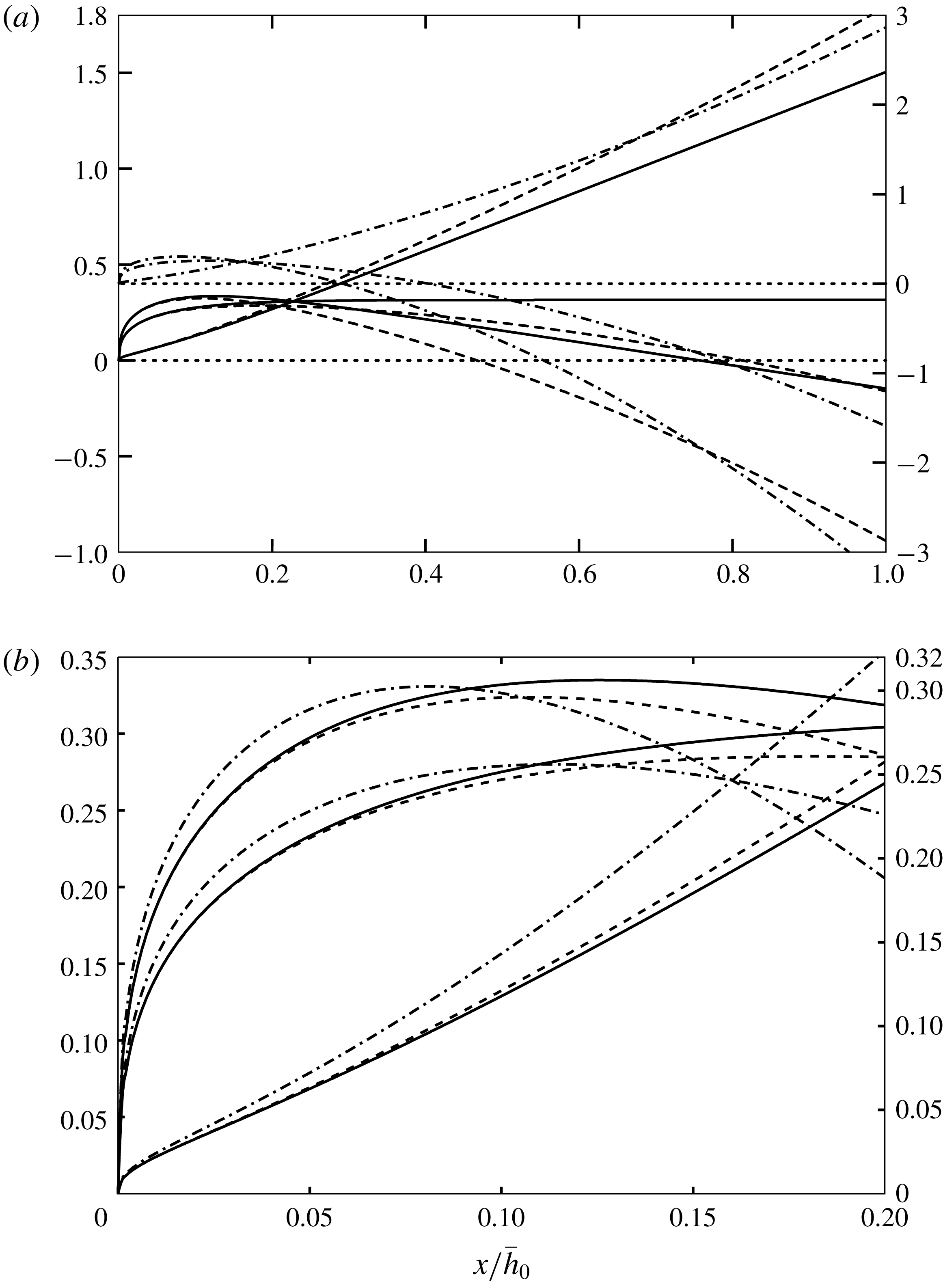
The accurate numerical evaluation of (3.25) for several values of
 $T$
and
 $\bar{g}$
is displayed in figure 4. We note that the first term on the right-hand side of (3.25) is negative and the second positive throughout. Remarkably,
 $\bar{h}_{-}$
changes abruptly sign as
 $T\rightarrow 1/2$
, accompanied by an unbounded deflection of the layer. Therefore, this special limit deserves a separate attention (beyond the scope of the current investigation).
Distributions of
 $\bar{h}_{-}$
versus
 $x/\bar{h}_{0}$
by (3.25); (a)
 $\bar{g}=0$
(solid, left ordinate),
 $\bar{g}=0.25$
(dashed, left ordinate),
 $\bar{g}=1$
(dot-dashed, right ordinate), each set for
 $T=0.2,0,1.2$
(bottom to top for
 $x/\bar{h}_{0}=1$
); (b) zoomed-in detail of (a); note that abscissae have a common origin.

In the context of (3.26), the solution of (3.2) has the following notable properties: the regular expansion
 $$\begin{eqnarray}\bar{\unicode[STIX]{x1D713}}_{0}\sim \unicode[STIX]{x1D706}z^{2}/2+\unicode[STIX]{x1D6FD}z^{5}+O(z^{8}),\quad z\rightarrow 0,\end{eqnarray}$$
with some constant
 $\unicode[STIX]{x1D6FD}$
(equal to
 $-\unicode[STIX]{x1D706}^{2}/60$
for Watson’s flow); the BCs imposed at
 $z=\bar{h}$
in (3.2b
) imply also
 $\bar{\unicode[STIX]{x1D713}}_{zzzz}(x,\bar{h})=0$
.
3.3.2 Far wake, downfall and ‘capillary ascent’
For
 $x\rightarrow \infty$
, the normalised streamwise-flow component
 $f_{\unicode[STIX]{x1D702}}\bar{h}_{0}/\bar{h}$
tends towards
 $\bar{h}_{0}/h_{\infty }$
as
 $h\sim \bar{h}$
attains some terminal value
 $h_{\infty }$
. In the
 $(x,z)$
-plane, it becomes horizontally aligned. Preservation of its streamwise momentum expressed by (3.5) confirms a contraction of the detached layer towards that uniform free jet:
 $h_{\infty }/\bar{h}_{0}\sim 1/(J_{0}\bar{h}_{0})<1$
. This constraint follows from the Cauchy–Schwarz or Jensen’s inequality and the conserved volumetric flow rate. Specifically, Watson’s flow passing the edge predicts
 $\bar{h}_{0}/h_{\infty }=\bar{h}_{0}J_{0}=a_{W}\unicode[STIX]{x1D706}\simeq 1.2570$
,
 $h_{\infty }/\bar{h}_{0}\simeq 0.7956$
. Linearising (3.2) about that ultimate flow state shows exponentially decaying and vertically oscillatory eigenmodes during the final stage of viscous diffusion:
 $$\begin{eqnarray}\left[\bar{\unicode[STIX]{x1D713}}-\frac{z}{h_{\infty }}-\mathop{\sum }_{n=1}^{\infty }a_{n}\text{e}^{-(n\unicode[STIX]{x03C0})^{2}x/h_{\infty }}\sin \left(\frac{n\unicode[STIX]{x03C0}z}{h_{\infty }}\right),\bar{h}-h_{\infty }\right]=O(\text{e}^{-2\unicode[STIX]{x03C0}^{2}x/h_{\infty }}),\end{eqnarray}$$
with the constants
 $a_{n}$
determined by the full solution to (3.8). The remainder term in (3.28) indicates that the higher-order eigenfunctions are dominated by the omitted contribution provoked by the nonlinear self-interaction of the dominant one.
For
 $g=0$
, (3.25) predicts
 $\bar{h}_{-}\sim a_{W}Tx/(2T-1)+O(1)$
(
 $x\rightarrow \infty$
), where the specific form of this linear growth is due to the continuity of
 $\bar{h}_{-}$
for
 $T=0$
at the plate edge. For any howsoever small value of
 $g$
, this behaviour is superseded by
 $\bar{h}_{-}\sim -\bar{g}x^{2}/[2J_{0}(1-2T)]+O(\bar{g}x,Tx)$
for
 $\bar{g}x^{2}$
becoming large. This reveals the classical downfall parabola which the essentially inviscid free layer assumes under sufficiently small capillary action. Increasing
 $T$
reinforces the vertical pressure gradient and thus the downward bending of the flow, cf. (3.3). Finally, as the value of
 $T$
exceeds
 $1/2$
, this feed-forward is replaced by an intriguing counteracting one: the flow curves more and more upwards in order to sustain a corresponding negative vertical pressure gradient increasingly dominated by surface tension. We thus consider the present results based upon (3.8) and (3.25) as the ‘viscous extension’ of the early ones by Keller & Weitz (Reference Keller and Weitz1957). Accordingly, boundedness of
 $\bar{h}_{-}$
for
 $x\rightarrow \infty$
occurs for
 $g=T=0$
solely: with
 $h_{\infty }=1/J_{0}$
and
 $K(\infty )=1/2$
, (3.25) yields in this limit when body and surface forces are ignored
 $$\begin{eqnarray}\frac{\bar{h}_{+}^{2}-\bar{h}_{-}^{2}}{2h_{\infty }}\sim \frac{\bar{h}_{\pm }}{h_{\infty }}\mp \frac{1}{2}\sim K_{W}+\frac{2}{\unicode[STIX]{x03C0}}\mathop{\sum }_{n=1}^{\infty }a_{n}\text{e}^{-(n\unicode[STIX]{x03C0})^{2}x/h_{\infty }}\frac{1-(-1)^{n}}{n}+O(\text{e}^{-2\unicode[STIX]{x03C0}^{2}x/h_{\infty }}).\end{eqnarray}$$
The left-most term in (3.29) obviously expresses the angular momentum around the plate edge exerted by the flow infinitely far downstream. We find
 $\bar{h}_{-}(\infty )\simeq 0.3157$
and
 $\bar{h}_{+}(\infty )\simeq 1.1121$
describing the terminal upwards shift of the detached layer.
Our careful numerical evaluations perfectly confirm the above findings: see figures 2(b) and 4.
3.3.3 Goldstein’s near wake and consequences
The analysis in this section substantially resorts to (3.27), but again without the need to specify
 $\bar{\unicode[STIX]{x1D713}}_{0}$
to represent Watson’s flow.
The sudden loss of the no-slip BC at the edge for
 $x\rightarrow 0+$
typically provokes a Goldstein-type near wake, with its vertical extent controlled by the local viscous length scale
 $x^{1/3}$
:
 $$\begin{eqnarray}\bar{\unicode[STIX]{x1D713}}/(\unicode[STIX]{x1D706}x^{2})^{1/3}\sim f_{G}(\unicode[STIX]{x1D701})+x^{\unicode[STIX]{x1D6FC}}f_{\unicode[STIX]{x1D6FC}}(\unicode[STIX]{x1D701})+O(x^{2\unicode[STIX]{x1D6FC}}),\quad \unicode[STIX]{x1D701}:=z(\unicode[STIX]{x1D706}/x)^{1/3}=O(1),\quad x\rightarrow 0+,\end{eqnarray}$$
 $\unicode[STIX]{x1D6FC}$
is some positive constant. The function
 $f_{G}$
is governed by the arising well-known leading-order problem
 $f_{G}^{\prime 2}-2f_{G}f_{G}^{\prime \prime }=3f_{G}^{\prime \prime \prime }$
,
 $f_{G}(0)=f_{G}^{\prime \prime }(0)=0$
and fixed uniquely by setting
 $f_{G}^{\prime \prime }(\infty )$
equal to
 $1$
by matching. This yields
 $f_{G}^{\prime }\sim \bar{\unicode[STIX]{x1D701}}+\,\text{transcendentally small terms}$
(TST) for
 $\bar{\unicode[STIX]{x1D701}}:=\unicode[STIX]{x1D701}+a_{G}\rightarrow \infty$
; our numerical computation of
 $f_{G}(\unicode[STIX]{x1D701})$
gives
 $a_{G}\simeq 0.8920$
. Hence,
 $$\begin{eqnarray}(2+3\unicode[STIX]{x1D6FC})(f_{G}^{\prime }f_{\unicode[STIX]{x1D6FC}}^{\prime }-f_{G}^{\prime \prime }f_{\unicode[STIX]{x1D6FC}})-2f_{G}f_{\unicode[STIX]{x1D6FC}}^{\prime \prime }=f_{\unicode[STIX]{x1D6FC}}^{\prime \prime \prime },\quad f_{\unicode[STIX]{x1D6FC}}(0)=f_{\unicode[STIX]{x1D6FC}}^{\prime \prime }(0)=0,\quad f_{\unicode[STIX]{x1D6FC}}^{\prime }(0)\neq 0,\end{eqnarray}$$
and
 $f_{\unicode[STIX]{x1D6FC}}=f_{G}^{\prime }$
satisfies only the first of these relationships. Thus,
 $f_{\unicode[STIX]{x1D6FC}}\sim \unicode[STIX]{x1D6FD}_{1}\bar{\unicode[STIX]{x1D701}}^{3\unicode[STIX]{x1D6FC}+2}+\unicode[STIX]{x1D6FD}_{2}\bar{\unicode[STIX]{x1D701}}+\text{TST}$
with some constants
 $\unicode[STIX]{x1D6FD}_{1,2}$
holds for
 $\bar{\unicode[STIX]{x1D701}}\rightarrow \infty$
. Rewriting (3.30) in terms of
 $x$
,
 $z$
yields
 $\unicode[STIX]{x1D6FC}=1$
,
 $\unicode[STIX]{x1D6FD}_{1}=\unicode[STIX]{x1D6FD}/\unicode[STIX]{x1D706}^{2}$
by (3.27) (
 $\unicode[STIX]{x1D6FD}_{1}=-1/60$
for Watson’s flow) via matching with
 $\bar{\unicode[STIX]{x1D713}}\sim \bar{\unicode[STIX]{x1D713}}_{0}$
(
 $z\gg x^{1/3}$
), and with (2.2d
) finally the sought irregular extension of the expansion (3.26) holding for
 $x\rightarrow 0+$
as
 $z=O(1)$
is found:
 $$\begin{eqnarray}\displaystyle [\bar{\unicode[STIX]{x1D713}}-\bar{\unicode[STIX]{x1D713}}_{0},\bar{h}-\bar{h}_{0}] & {\sim} & \displaystyle ax^{1/3}[\bar{\unicode[STIX]{x1D713}}_{0}^{\prime },-1]+a^{2}x^{2/3}[\bar{\unicode[STIX]{x1D713}}_{0}^{\prime \prime }/2,0]+x[a^{3}\bar{\unicode[STIX]{x1D713}}_{0}^{\prime \prime \prime }/6+\bar{\unicode[STIX]{x1D713}}_{1}(z),\bar{h}_{1}]\nonumber\\ \displaystyle & & \displaystyle +\,O(x^{4/3}),\quad a:=a_{G}/\unicode[STIX]{x1D706}^{1/3}\simeq 1.0079,\end{eqnarray}$$
with that numerical value valid for Watson’s flow. The detaching flow stays intact immediately downstream of the edge apart from being slightly perturbed by a local eigensolution
 $x^{1/3}\bar{\unicode[STIX]{x1D713}}^{\prime }$
of (3.2a
) as in (3.14a
); this inviscid-flow disturbance is triggered by the displacement of Goldstein’s wake forming underneath.
From (3.30) and (3.32), the dominant contribution to
 $z=\bar{h}_{-}(x)$
in (3.25) as
 $x\rightarrow 0+$
originates in the core layer
 $z=O(1)$
. The layer responds to the capillary jumps of the pressure and its cross-flow variation by streamline curvature in terms of a cuspidal bending, confirmed by the numerical results shown in figure 4(b) and visualised in figure 5(a):
 $$\begin{eqnarray}[\bar{h}_{-},\bar{h}_{+}]\sim [1-T,T]ax^{1/3}/(1-2T)+O(x^{2/3}),\end{eqnarray}$$
with
 $T$
defined in (3.16c
). In addition to the case
 $T=1/2$
, we also discard the further physically exceptional, degenerate one
 $T=1$
, which marks the onset of capillary undulations above the plate (§ 3.2.2). The layer contracts, i.e. accelerates, almost independently of
 $T$
in agreement with (3.32) and the numerical results (figure 2
b) as free slip supersedes no slip at its base. For
 $T>0$
, the inverse Prandtl shift produces additional irregular terms in the core region for
 $x\rightarrow 0+$
, defining a cuspidal distortion of
 $h_{+}$
originating from the near wake. The hydrostatically caused
 $O(x^{2})$
-contribution to
 $\bar{h}_{-}$
in (3.3) arises from both
 $f_{G}$
for
 $z=O(x^{1/3})$
and the regular part of (3.32) for
 $z=O(1)$
.
Goldstein’s wake; (a) local distributions of
 $\bar{h}_{-}^{\prime }/(ax^{1/3})$
(solid),
 $\bar{h}_{+}/(ax^{1/3})$
(dashed) versus
 $T$
with zeros and asymptotes (dotted) as given by (3.33); (b)
 $F_{G}^{\prime }(\unicode[STIX]{x1D701})$
(solid),
 $f_{G}^{\prime }(\unicode[STIX]{x1D701})$
(dashed), median as asymptote
 $F_{G}^{\prime }\sim \unicode[STIX]{x1D701}$
(dotted).

Exploiting (3.3) and (3.33) gives for
 $x\rightarrow 0+$
 $$\begin{eqnarray}\bar{p}-\bar{p}(0,z)\sim \frac{T}{2T-1}\left(\frac{J(z)}{J(0)}-T\right)\frac{2a}{9}x^{-5/3}+O(x^{-4/3}),\quad J(z):=\int _{z}^{\bar{h}_{0}}\bar{\unicode[STIX]{x1D713}}_{0}^{\prime 2}(y)\,\text{d}t,\end{eqnarray}$$
so henceforth,
 $J(0)=J_{0}$
. In order to estimate
 $\bar{p}$
in the near wake, the integral in (3.3) has to be split asymptotically. With the aid of (3.7) and with
 $(\ast )$
abbreviating the integrand in (3.3) of
 $O(x^{-1})$
, one obtains
 $\bar{p}-\unicode[STIX]{x1D70F}\bar{h}_{-}^{\prime \prime }\sim \int _{0}^{z}(\ast )\,\text{d}t-\bar{\unicode[STIX]{x1D713}}_{zx}-\bar{\unicode[STIX]{x1D713}}_{zx,-}+\bar{\unicode[STIX]{x1D713}}_{zz}\bar{h}_{-}^{\prime \prime }=O(x^{-2/3})$
for
 $z=O(x^{1/3})$
. As Watson’s flow having
 $\text{d}\bar{p}_{p}/\text{d}x\equiv 0$
provides the regular extension of (3.26), regular pressure terms contribute to (3.30) and in turn induce contributions to (3.32) at higher orders only.
It is seen that gravity has no essential impact on the behaviour of the just detaching film given the magnitude of the Froude numbers considered. However, we find the following two sources of non-uniformity of the above expansions.
(I) In the case
$\unicode[STIX]{x1D70F}=0$
, we conclude that in the parabolic slender-flow limit Watson’s classical flow is abruptly superseded by Goldstein’s one at the trailing edge. The irregular shape of the detaching streamline reflects the absence of any upstream influence. However, in the region
$x=O(\unicode[STIX]{x1D716}^{3/2})$
,
$y=O(\unicode[STIX]{x1D716}^{1/2})$
encompassing the edge and where
$[\unicode[STIX]{x1D713},p,h_{-}]=O(\unicode[STIX]{x1D716})$
the slender-layer approximation anticipated in (2.2c,d
) ceases to be valid, and all terms in (2.2), apart from
$-g$
in (2.2b
), are retained to leading order. Most important, the solution to this full NS problem is expected to facilitate a smooth transition from no-slip to free-slip, according to (2.2c
). This then completes the current flow description (§ 4.1).(II) For any howsoever small values of
$\unicode[STIX]{x1D70F}$
, even the upper streamline exhibits an unacceptable cusp for
$x\rightarrow 0+$
, which cannot be smoothed out by the aforementioned NS region. We observe that
$\bar{p}=O(\unicode[STIX]{x1D70F}x^{-5/3})$
in the near wake for
$x\ll \unicode[STIX]{x1D70F}$
and the magnitude of
$\bar{p}_{p}$
immediately upstream of the edge can only be increased accordingly by the action of viscous forces. Consequently, the required smoothing of the flow quantities in the vicinities of both the edge as well the upper free streamline is typically accomplished by viscous–inviscid interaction due to streamline curvature, as identified in § 3.2.2: on a reduced streamwise length scale of
$O(\unicode[STIX]{x1D716}^{6/7})$
between the flow in the lower deck (LD), continued as the near wake further downstream, where
$z=O(\unicode[STIX]{x1D716}^{2/7})$
and the predominantly inviscid one in the main deck (MD) comprising the core region. As shown next, this loss of parabolicity, with the slender-layer approximation staying intact first, completes the flow picture for
$p$
– and thus
$g\bar{h}$
– becoming of
$O(\unicode[STIX]{x1D716}^{4/7})$
. So
$g$
is increased above
$O(\unicode[STIX]{x1D716}^{2})$
and the distinguished limit (3.4) relaxed accordingly.





4 Interactive stage
We now modify the flow structure on the shorter scale introduced in (II) above such that the vertical momentum transport compensates for an correspondingly increased pressure variation accommodating the capillary pressure jump. Simultaneously, the hydrostatic contribution to the thereby modified plate pressure is enhanced accordingly. Let us describe this regime of strong local interaction, which facilitates the necessary upstream influence, canonically by rescaled quantities of
 $O(1)$
denoted by uppercase letters.
4.1 Interaction problem: discussion and preliminary findings
To enhance the clarity of the scalings involved, we relax Watson’s representation
 $J_{0}=\unicode[STIX]{x1D706}$
of the incident flow and define (with the case
 $T=1$
excluded)
 $$\begin{eqnarray}G:=\unicode[STIX]{x1D716}^{-4/7}g\bar{h}_{0}/(M^{2}\unicode[STIX]{x1D706}^{6})^{1/7},\quad M:=|T-1|J_{0},\quad S:=\text{sgn}(T-1).\end{eqnarray}$$
The first definition parametrises the distinguished limit indicated above by taking
 $G$
to be of
 $O(1)$
to require upstream adjustment. In the LD, (2.2a
) reduces to slender-layer form, where a streamwise pressure gradient dictates the massive modification of the unperturbed oncoming flow towards Goldstein’s wake flow. The LD is characterised by
 $$\begin{eqnarray}\displaystyle \displaystyle [X,Z] & := & \displaystyle [(\unicode[STIX]{x1D706}^{5}/M^{3})^{1/7}x/\unicode[STIX]{x1D716}^{6/7},(\unicode[STIX]{x1D706}^{4}/M)^{1/7}z/\unicode[STIX]{x1D716}^{2/7}],\end{eqnarray}$$
 $$\begin{eqnarray}\displaystyle \displaystyle [\unicode[STIX]{x1D713},p]/\unicode[STIX]{x1D716}^{4/7} & {\sim} & \displaystyle [(M^{2}/\unicode[STIX]{x1D706})^{1/7}\unicode[STIX]{x1D6F9}(X,Z),(M^{2}\unicode[STIX]{x1D706}^{6})^{1/7}P(X)]+O(\unicode[STIX]{x1D716}^{6/7}).\end{eqnarray}$$
Here the asymptotic remainder can be determined by the same matching arguments specifying
 $\unicode[STIX]{x1D6FC}=1$
in (3.30). In the LD, we then have in accordance with (3.2) typically
 $$\begin{eqnarray}\displaystyle & \displaystyle \unicode[STIX]{x1D6F9}_{Z}\unicode[STIX]{x1D6F9}_{ZX}-\unicode[STIX]{x1D6F9}_{X}\unicode[STIX]{x1D6F9}_{ZZ}=-P^{\prime }+\unicode[STIX]{x1D6F9}_{ZZZ}, & \displaystyle\end{eqnarray}$$
 $$\begin{eqnarray}\displaystyle & \displaystyle Z=0:\quad \unicode[STIX]{x1D6F9}=\unicode[STIX]{x1D6F9}_{Z}\unicode[STIX]{x1D703}(-X)=\unicode[STIX]{x1D6F9}_{ZZ}\unicode[STIX]{x1D703}(X)=0, & \displaystyle\end{eqnarray}$$
 $$\begin{eqnarray}\displaystyle & \displaystyle X\rightarrow -\infty :\quad \unicode[STIX]{x1D6F9}_{Z}\rightarrow Z,\quad Z\rightarrow \infty :\quad \unicode[STIX]{x1D6F9}_{Z}-Z\rightarrow A(X). & \displaystyle\end{eqnarray}$$
 $-A(X)$
describes the vertical displacement exerted there.
To the approximation required, (2.2a,b ) reduce to the Euler equations in the MD, then conveniently written as
 $$\begin{eqnarray}\unicode[STIX]{x1D713}_{z}^{2}(\unicode[STIX]{x1D713}_{x}/\unicode[STIX]{x1D713}_{z})_{z}=h_{-}^{\prime }p_{z}-p_{x},\quad (\unicode[STIX]{x1D716}\unicode[STIX]{x1D713}_{z})^{2}[(\unicode[STIX]{x2202}_{x}-h_{-}^{\prime }\unicode[STIX]{x2202}_{z})(\unicode[STIX]{x1D713}_{x}/\unicode[STIX]{x1D713}_{z})-\bar{h}_{-}^{\prime \prime }]=p_{z}+g\end{eqnarray}$$
with the Prandtl shift invoked. These together with the rationale underlying (3.32) imply
 $$\begin{eqnarray}\displaystyle & & \displaystyle [\unicode[STIX]{x1D713},h,h_{-},h_{+},p]\sim [\bar{\unicode[STIX]{x1D713}}_{0},\bar{h}_{0},0,\bar{h}_{0},0]+(\unicode[STIX]{x1D716}^{2}M/\unicode[STIX]{x1D706}^{4})^{1/7}[A\bar{\unicode[STIX]{x1D713}}_{0}^{\prime },-A,H_{-},H_{+},0]\nonumber\\ \displaystyle & & \displaystyle \quad +\,(\unicode[STIX]{x1D716}^{2}M/\unicode[STIX]{x1D706}^{4})^{2/7}[\unicode[STIX]{x1D713}_{2}(X,z),H_{2},H_{2,-},H_{2,-}+H_{2},\unicode[STIX]{x1D706}^{2}\bar{P}(X,z)]+O(\unicode[STIX]{x1D716}^{6/7}).\end{eqnarray}$$
Here
 $A(X)$
,
 $H_{-}(X)$
, and the (insignificant) term
 $H_{2,-}(X)$
are initially unknown,
 $A$
decays far upstream and the remaining perturbation quantities read
 $$\begin{eqnarray}\left.\begin{array}{@{}c@{}}\displaystyle \unicode[STIX]{x1D713}_{2}:=\frac{A^{2}}{2}\bar{\unicode[STIX]{x1D713}}_{0}^{\prime \prime }+\frac{\unicode[STIX]{x1D706}^{2}G}{\bar{h}_{0}}\unicode[STIX]{x1D713}_{g}(0,z)+H_{+}^{\prime \prime }\bar{\unicode[STIX]{x1D713}}_{0}^{\prime }\left[\unicode[STIX]{x1D706}^{2}\int _{0}^{z}\left(\frac{T-J(t)/J_{0}}{|T-1|\bar{\unicode[STIX]{x1D713}}_{0}^{\prime 2}(t)}-\frac{S}{(\unicode[STIX]{x1D706}t)^{2}}\right)\text{d}t-\frac{S}{z}\right],\\ \displaystyle \left.H_{+}:=H_{-}-A,\quad H_{2}:=-\frac{\unicode[STIX]{x1D713}_{2}}{\bar{\unicode[STIX]{x1D713}}_{0}^{\prime }}\right|_{z=\bar{h}_{0}},\quad \bar{P}:=\frac{H_{+}^{\prime \prime }(X)}{|T-1|}\left(\frac{J(z)}{J_{0}}-T\right)-G\left(\frac{z}{\bar{h}_{0}}-1\right).\end{array}\right\}\end{eqnarray}$$
Matching (4.6) with (4.3) is provided by the eigensolutions contributing to
 $\unicode[STIX]{x1D713}_{1,2}$
and with (3.1) by integration over
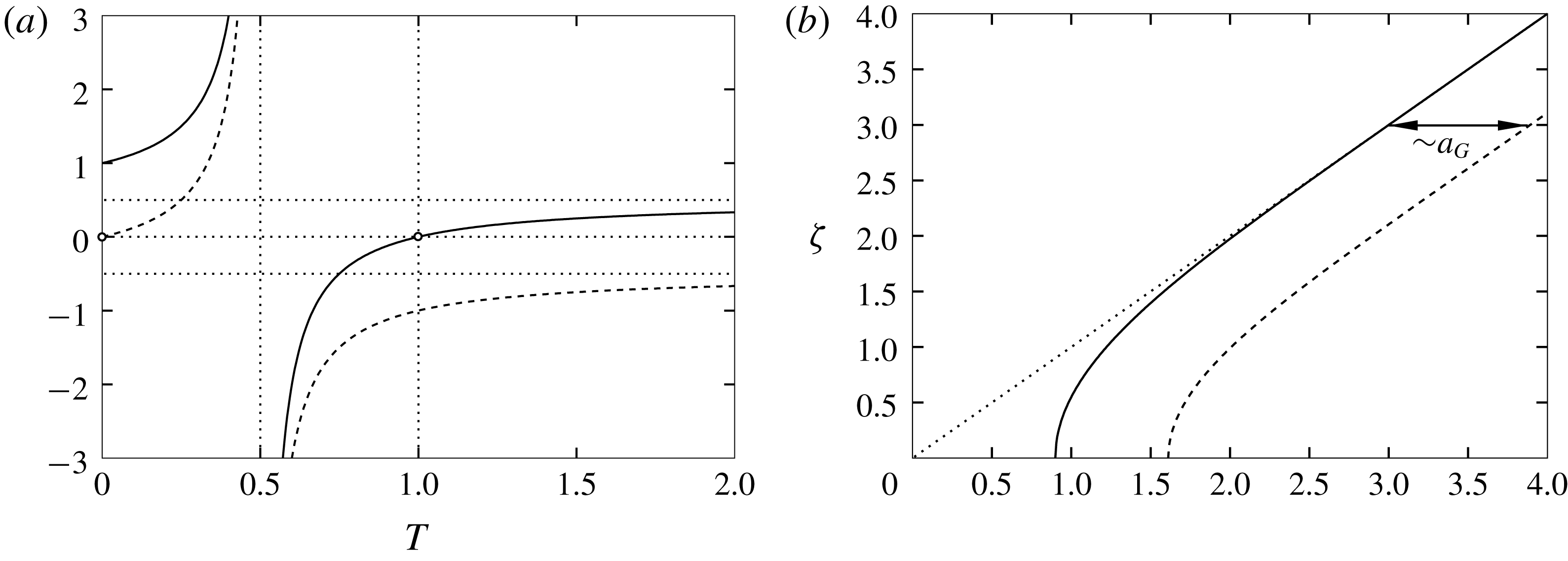
 $X$
(and employing the upstream perturbation
 $\unicode[STIX]{x1D713}_{g}$
of Watson’s flow). The pressure function
 $\bar{P}$
results from integrating
 $\bar{P}_{z}$
balancing the streamline curvature subject to
 $\bar{P}(X,\bar{h}_{0})=-TH_{+}^{\prime \prime }/|T-1|$
, see (2.2b,d
). The kinematic BCs (2.2c
) fix the expansion of
 $h$
in (4.6). Since viscous shear enters (4.6) not earlier than at
 $O(\unicode[STIX]{x1D716}^{6/7})$
, the incident portion
 $\bar{\unicode[STIX]{x1D713}}_{0}^{\prime \prime }+g\unicode[STIX]{x2202}_{zz}\unicode[STIX]{x1D713}_{g}$
of the vorticity
 $\unicode[STIX]{x1D713}_{yy}+\unicode[STIX]{x1D716}^{2}\unicode[STIX]{x1D713}_{xx}$
is preserved along the streamlines of the inviscid flow described by the explicit part of (4.6). On the interactive scale,
 $\unicode[STIX]{x1D716}^{2}\unicode[STIX]{x1D713}_{xx}(x,\bar{h})\sim -(\unicode[STIX]{x1D716}^{4}\unicode[STIX]{x1D706}^{6}/M^{5})^{1/7}H_{+}^{\prime \prime }\bar{\unicode[STIX]{x1D713}}_{0}^{\prime }(\bar{h}_{0})+O(\unicode[STIX]{x1D716}^{6/7})$
. Hence, the first of the dynamic BCs (2.2d
) is satisfied identically, cf. (3.11), only up to contributions of
 $O(\unicode[STIX]{x1D716}^{2/7})$
; the expressions in (4.7) imply a contradiction. However, the required thin surface shear layer only plays a subordinate role subsequently and is therefore ignored. We just estimate its lateral extent: inspection of (2.2a
) shows that in this layer
 $h_{+}-y$
is typically measured by the square root of the streamwise length scale given by
 $\unicode[STIX]{x1D716}^{6/7}$
. It is thus much thicker than the LD but adjusts to variations of
 $h_{+}$
according to (4.6). There also the regular part of the expansion (3.32) is recovered and the smooth continuation of
 $h_{+}$
across the edge guaranteed on smaller streamwise scales.
Matching (4.3) and (4.6) yields specifically
 $\unicode[STIX]{x1D6F9}\sim (Z+A)^{2}/2+P-G+\text{TST}$
(
 $Z\rightarrow \infty$
) and
 $P(X)=\bar{P}(X,0)$
. This together with (2.2d
) furnishes the interaction law
 $$\begin{eqnarray}P-G=S(A-H_{-})^{\prime \prime },\quad P\unicode[STIX]{x1D703}(X)=TH_{-}^{\prime \prime }/|T-1|.\end{eqnarray}$$
The relationships (4.8) close (4.4) to establish a free-interaction problem determining
 $\unicode[STIX]{x1D6F9}$
,
 $P$
,
 $H_{-}$
and in turn
 $\bar{P}$
, parametrised by
 $G$
and
 $T$
, once the requirements of a sufficiently smooth behaviour at
 $X=0$
are established. The present problem represents a modification of its precursors devised by Smith (Reference Smith1977) and Bowles & Smith (Reference Bowles and Smith1992) in their study on the onset of very strong hydraulic jumps, i.e. in very supercritical flow, where the hydrostatic pressure varies only weakly. In sharp contrast, it here is altered massively by streamline curvature by virtue of a process reinforced in the downstream direction as described by (4.8). Below, we highlight the behaviour of the interactive flow in close vicinity to the trailing edge in appropriate detail. This cornerstone of our analysis also points to the construction of full numerical solutions of the problem, with their portion for
 $x<0$
presented in § 4.2 below.
It is first recognised that (4.4a
) yields for
 $X\rightarrow -\infty$
typically
 $$\begin{eqnarray}\left[\unicode[STIX]{x1D6F9}-\frac{Z^{2}}{2},P-G\right]\sim \unicode[STIX]{x1D6E4}\text{e}^{\unicode[STIX]{x1D707}X}\left[3\unicode[STIX]{x1D707}^{1/3}\int _{0}^{Z}(Z-t)\text{Ai}(\unicode[STIX]{x1D707}^{1/3}t)\,\text{d}t,\frac{-3^{2/3}}{\unicode[STIX]{x1D707}^{1/3}\unicode[STIX]{x0393}(\frac{1}{3})}\right]+\text{c.c.}+O(\text{e}^{2\unicode[STIX]{x1D707}X}),\end{eqnarray}$$
with some eigenvalue
 $\unicode[STIX]{x1D707}$
having
 $\text{Re}\,\unicode[STIX]{x1D707}>0$
and some constant
 $\unicode[STIX]{x1D6E4}$
. The asymptotic forms
 $A\sim \unicode[STIX]{x1D6E4}\text{e}^{\unicode[STIX]{x1D707}X}+\text{c.c.}$
(
 $\unicode[STIX]{x1D6E4}\neq 0$
) and
 $P\sim SA^{\prime \prime }$
are both satisfied if
 $$\begin{eqnarray}\unicode[STIX]{x1D707}=3^{2/7}/[-S\unicode[STIX]{x0393}(1/3)]^{3/7}\simeq 0.8972/(-S)^{3/7}.\end{eqnarray}$$
We arrive at a unique positive value of
 $\unicode[STIX]{x1D707}$
for
 $T<1$
and
 $\unicode[STIX]{x1D707}=|\unicode[STIX]{x1D707}|\exp (-3\text{i}\unicode[STIX]{x03C0}/7)$
, meaning a wavy upstream tail of the flow quantities, in the capillarity-dominated case
 $T>1$
. Any non-zero value of
 $\unicode[STIX]{x1D6E4}$
controls the interactive flow uniquely as long as it stays attached. Most important, by (3.24) and (3.22), the expansions (4.3) and (3.16) are found to match so that the SL in § 3.2.2 is superseded by the LD provided
 $$\begin{eqnarray}\unicode[STIX]{x1D6FE}_{0}=\unicode[STIX]{x1D6E4}\unicode[STIX]{x1D6E5}(\unicode[STIX]{x1D716};0).\end{eqnarray}$$
Hence,
 $\unicode[STIX]{x1D6E4}$
is real (complex) for
 $T<1$
(
 $T>1$
). In other words, once the value of
 $\unicode[STIX]{x1D6E4}=O(1)$
has been determined as is shown below, it fixes
 $\unicode[STIX]{x1D6FE}_{0}=O(\unicode[STIX]{x1D716}^{2/7})$
in (3.18). Simultaneously, (3.16) ceases to be valid for
 $x=O(\unicode[STIX]{x1D716}^{6/7})$
. That value of
 $\unicode[STIX]{x1D6FE}_{0}$
in turn selects a specific member in the class of eigensolutions studied in § 3.2.2. This demonstrates a strong, nonlinear continuation of the interaction mechanism addressed in § 3.2.2, (ii), subject to (3.19) (
 $T<1$
), (3.23) (
 $T>1$
) and (3.24), where Watson’s solution represents the background flow (the essential constraints are the linear streamwise variation of
 $P_{\unicode[STIX]{x1D716}}$
in (3.16c
) and
 $J_{0}=\unicode[STIX]{x1D706}$
).
The history of the linearised eigensolutions given by (4.9) can be traced back to the virtual origin
 $x=-1$
through (3.18) and (3.20). Alternatively, the for
 $x>-1$
exponential growth of the eigensolutions in § 3.2.2 renders the fully nonlinear interaction mechanism around the edge admissible – an instructive interpretation of its upstream influence.
The possible interactive flows adjacent to the plate are identified on the basis of (4.8). When we ignore the restriction
 $X<0$
imposed on the marching problem formed by (4.4), (4.8) and (4.9), it is invariant against an origin shift whereby
 $X$
is replaced by
 $$\begin{eqnarray}X_{s}:=X+\ln |\unicode[STIX]{x1D6E4}|/\text{Re}\unicode[STIX]{x1D707}.\end{eqnarray}$$
Accordingly, in (4.9) we substitute
 $$\begin{eqnarray}\unicode[STIX]{x1D6E4}\exp (\unicode[STIX]{x1D707}X)=\exp (\unicode[STIX]{x1D707}X_{s}+\text{i}\unicode[STIX]{x1D719}),\quad \unicode[STIX]{x1D719}:=\arg \unicode[STIX]{x1D6E4}+\left\{\begin{array}{@{}ll@{}}\displaystyle 0 & (T<1),\\ \tan (3\unicode[STIX]{x03C0}/7)\ln |\unicode[STIX]{x1D6E4}|\quad \text{mod}\;2\unicode[STIX]{x03C0} & (T>1).\end{array}\right.\end{eqnarray}$$
For
 $T<1$
, one takes
 $\unicode[STIX]{x1D6E4}$
as real where
 $\unicode[STIX]{x1D6E4}>0$
(
 $\unicode[STIX]{x1D6E4}<0$
) triggers an expansive (compressive, cf. Smith & Duck Reference Smith and Duck1977) flow giving
 $P^{\prime }<0$
(
 $P^{\prime }>0$
). Here (4.13) yields two canonical solutions, only differing by
 $\text{sgn}\,\unicode[STIX]{x1D6E4}$
. Solely for
 $\unicode[STIX]{x1D6E4}>0$
, this terminates in well-established singular fashion at some finite value of
 $X_{s}$
we designate as
 $X_{s}^{t}$
(Smith Reference Smith1977; Bowles & Smith Reference Bowles and Smith1992). Essentially, the LD splits with a predominantly inviscid core flow of constant shear that induces a viscous slip layer adjacent to the plate. Casting the original analysis of this singularity by Smith (Reference Smith1977) in the present scaling, we find the following behaviour of the key quantities
 $A$
,
 $P$
and the shear rate at the plate
 $\unicode[STIX]{x1D6F4}:=\unicode[STIX]{x1D6F9}_{ZZ}(X,0)$
for
 $\unicode[STIX]{x0394}X:=X_{s}-X_{s}^{t}\rightarrow 0-$
:
 $$\begin{eqnarray}A\sim 12/(\unicode[STIX]{x0394}X)^{2},\quad G-P\sim 72/(\unicode[STIX]{x0394}X)^{4},\quad \unicode[STIX]{x1D6F4}\sim 24\sqrt{6}\unicode[STIX]{x1D712}/(-\unicode[STIX]{x0394}X)^{7/2},\quad \unicode[STIX]{x1D712}\simeq 1.1736.\end{eqnarray}$$
Herein,
 $\unicode[STIX]{x1D712}$
is determined by the numerical solution of the Falkner–Skan problem governing the slip layer. These findings were confirmed qualitatively by the numerical study of Bowles & Smith (Reference Bowles and Smith1992) (see figure 7a therein).
On the other hand, for
 $T>1$
, both
 $\text{Re}\,\unicode[STIX]{x1D6E4}$
and
 $\text{Im}\,\unicode[STIX]{x1D6E4}$
, see (4.9) and (4.13), parametrise the interactive-flow regime upstream of the edge. The origin shift condenses these two degrees of freedom into the phase shift
 $\unicode[STIX]{x1D719}$
(
 $0\leqslant \unicode[STIX]{x1D719}<2\unicode[STIX]{x03C0}$
) of the harmonic modulation in (4.13). Investigated extensively by Bowles & Smith (Reference Bowles and Smith1992) for
 $G=0$
(in terms of a capillarity-dominated limit, see figure 6 therein), in this case the curvature of the surface, expressed through
 $-A^{\prime \prime }(X)$
, induces a pressure response of opposite sign such that the flow becomes increasingly oscillatory in the downstream direction. Those authors found that eventually separation occurs, which has the numerical marching scheme intrinsically terminate as the wall friction becomes sufficiently negative. Unfortunately, the quite marked dependence of their results on the spatial discretisation hampers their more conclusive discussion. As being of relevance to what follows, however, see § 4.2.3, they concluded that
 $P$
must attain a finite negative plateau for
 $X_{s}$
becoming large.
Initiated by (4.9), downstream marching is deemed to generate a regular behaviour of
 $\unicode[STIX]{x1D6F9}$
and
 $P$
as
 $X\rightarrow 0-$
. The absence of a further regularising interactive mechanism at play on some reduced
 $X$
-scale requires continuity of
 $\unicode[STIX]{x1D6F9}$
,
 $P$
,
 $H_{-}$
at the edge; and in turn of
 $A$
,
 $\bar{P}$
,
 $H_{+}=H_{-}-A$
and
 $H_{+}^{\prime \prime }$
. The rationale predicting continuity of the regular expansion of
 $\bar{h}_{+}^{\prime }$
in § 3.3.3, accomplished by terms of
 $O(\unicode[STIX]{x1D716}^{6/7})$
in (4.6), predicts continuity of
 $H_{+}^{\prime }$
too. With
 $\unicode[STIX]{x1D6F9}_{0}:=\unicode[STIX]{x1D6F9}(0,Z)$
, (4.4) yields for
 $X\rightarrow 0-$
, as a counterpart to (3.26),
 $$\begin{eqnarray}\unicode[STIX]{x1D6F9}-\unicode[STIX]{x1D6F9}_{0}\sim X\unicode[STIX]{x1D6F9}_{0}^{\prime }R(Z)+O(X^{2}),\quad R(Z):=\int _{0}^{Z}\frac{\unicode[STIX]{x1D6F9}_{0}^{\prime \prime \prime }(t)-P^{\prime }(0-)}{\unicode[STIX]{x1D6F9}_{0}^{\prime 2}(t)}\,\text{d}t,\quad A^{\prime }(0-)=R(\infty ).\end{eqnarray}$$
However, the inevitable discontinuous drop of the edge shear rate from
 $\unicode[STIX]{x1D6EC}(\unicode[STIX]{x1D6E4}):=\unicode[STIX]{x1D6F9}_{ZZ}(0-,0)$
to zero and (4.4a,b
) reinstate a Goldstein-type wake at the base of the LD, by analogy with (3.30). This is smoothed though on the smaller scales reinvoking the NS region envisaged in § 3.3.3, (I), where
 $X=O(\unicode[STIX]{x1D716}^{9/14})$
. Matching
 $p$
then requires
 $P(0)=0$
, even for finite values of
 $T$
, but not necessarily continuity of
 $P^{\prime }$
at
 $X=0$
. Since the full NS solution also accounts for the capillary pressure jump, we have
 $\unicode[STIX]{x1D70F}h_{-}\lesssim O(\unicode[STIX]{x1D716}^{2})$
in that regime (irrespective of the static contact angle). For
 $$\begin{eqnarray}\unicode[STIX]{x1D716}^{9/14}\ll X\ll \min (T^{3/8},1)\end{eqnarray}$$
one infers
 $TH_{-}\lesssim X^{8/3}$
by matching, as already absorbed by (4.8), and thus
 $P\lesssim X^{2/3}$
. We thereby arrive at the sought supplementary, and sufficient, edge conditions
 $$\begin{eqnarray}\unicode[STIX]{x1D6F9}(0-,Z)=\unicode[STIX]{x1D6F9}(0+,Z),\quad H_{+}^{\prime }(0-)=H_{+}^{\prime }(0+),\quad TH_{-}^{\prime }(0)=H_{-}(0)=P(0)=0.\end{eqnarray}$$
With the use of (4.7) and
 $H_{1}:=-A^{\prime }(0-)=H_{+}^{\prime }(0)$
, thus integration of (4.8) finally yields
 $$\begin{eqnarray}A(X)=A(0)-H_{1}X+(2T-1)/(T-1)H_{-}(X)-SGX^{2}/2\quad (X\geqslant 0).\end{eqnarray}$$
4.2 Interaction problem: solutions for upstream flow
The very last of the requirements (4.17),
 $P(0)=0$
, specifies the role of the upstream influence. It fixes the required value of
 $\unicode[STIX]{x1D6E4}$
,
 $\unicode[STIX]{x1D6E4}_{0}$
say, and, according to (4.11),
 $\unicode[STIX]{x1D6FE}_{0}$
so as to achieve a pressure drop
 $G$
from
 $X=-\infty$
. Its impact differs strongly in the two pivotal cases depending on
 $S$
as summarised above and resumed as follows, accompanied by a thorough numerical investigation of (4.4) subject to (4.8) and (4.9) (of higher precision than the related results put forward by Bowles & Smith Reference Bowles and Smith1992). This is also stimulated by the demand for predicting most accurately the behaviour of the flow immediately upstream of the edge as this feeds into the interactive portion of the free layer (
 $X>0$
). We concentrate here on the plate region
 $X<0$
, leaving the solution for
 $X>0$
for a separate study. It is noteworthy that the solutions of free-interaction problems involving different linear local interaction laws bear interesting resemblances to the peculiarities of the present solutions discussed below: cf. Rothmayer (Reference Rothmayer1989) in connection with the expansive case and Rothmayer & Levine (Reference Rothmayer and Levine1991) with the compressive one; cf. also Gajjar & Smith (Reference Gajjar and Smith1983).
4.2.1 Solution strategy
Downstream integration was performed with the same method, routine and precision as in § 3.3. To this end, (4.4a
) together with (4.8) are formulated as a system of first-order equations with respect to
 $X_{s}$
. We prescribed the second of the conditions (4.4c
) at a sufficiently large maximum value of
 $Z$
. A sufficiently small (and for
 $T<1$
negative) initial value
 $P^{i}$
, say, of the difference pressure
 $P-G$
triggers the exponential departure, where
 $X_{s}$
takes on some correspondingly large negative value
 $X_{s}^{i}$
, say. Noting that (4.10) implies
 $-3^{2/3}/[\unicode[STIX]{x1D707}^{1/3}\unicode[STIX]{x0393}(1/3)]=S\unicode[STIX]{x1D707}^{2}$
and taking the explicit expression for
 $P$
in (4.9) as real gives in combination with (4.1) and (4.13)
 $\exp (\unicode[STIX]{x1D707}X_{s}^{i}+\text{i}\unicode[STIX]{x1D719})=P^{i}/(2S\unicode[STIX]{x1D707}^{2})$
. Then the initial kick for
 $\unicode[STIX]{x1D6F9}$
is readily calculated upon substitution of the exponential and integration. Moreover, this representation of
 $P^{i}$
yields
 $$\begin{eqnarray}X_{s}^{i}=\ln |P^{i}/(2\unicode[STIX]{x1D707}^{2})|/\text{Re}\unicode[STIX]{x1D707},\quad \unicode[STIX]{x1D719}=\arg (P^{i}/S)-2\arg \unicode[STIX]{x1D707}-X_{s}^{i}\text{Im}\,\unicode[STIX]{x1D707}\quad \text{mod}\;2\unicode[STIX]{x03C0}\end{eqnarray}$$
to determine
 $\unicode[STIX]{x1D719}$
as a function of
 $P^{i}$
in the oscillatory case
 $T>1$
. Here implementing the classical FLARE technique (Reyhner & Flügge-Lotz Reference Reyhner and Flügge-Lotz1968) helped to stabilise downstream integration when it comes to flow reversal.
The remaining details of the adopted discretisation differ in the two distinct cases and are therefore specified below. The thereby obtained results are not significantly altered by any substantial refinement of the resolution, as became evident through rather elaborate numerical tests. Consequently, those were accepted as essentially resolution-independent and sufficiently accurate. The solution is considered on consecutive
 $X_{s}$
-steps of 0.05.
4.2.2 Canonical expansive case:
$T<1$

As outlined before, in this gravity-dominated case only the expansive branching (4.9) enables the local acceleration of the flow towards the edge required by
 $P=0$
there. According to (4.13), this together with
 $\unicode[STIX]{x1D6E4}_{0}$
is found by a single numerical downstream sweep over
 $X_{s}>-\infty$
. It yields
 $P-G<0$
as a strictly monotonically decreasing function of
 $X_{s}$
solely. In turn, the terminal value of
 $X_{s}$
indicating the plate edge (
 $X=0$
) and, by (4.12),
 $\unicode[STIX]{x1D6E4}_{0}$
are strictly monotonically increasing functions of
 $G$
. We then write
 $\unicode[STIX]{x1D6E4}_{0}(G)$
with
 $\unicode[STIX]{x1D6E4}_{0}(0)=0$
, tied in with the trivial solution
 $\unicode[STIX]{x1D6F9}-Z\equiv P\equiv H_{+}\equiv 0$
, and expect some maximum value
 $\unicode[STIX]{x1D6E4}_{0}(\infty )=\exp (\unicode[STIX]{x1D707}X_{s}^{t})$
where the position of the intrinsic expansive breakdown described by (4.14) has approached
 $X=0$
from above. Only values of
 $\unicode[STIX]{x1D6E4}_{0}$
less than this prove meaningful within the framework of the current theory.
It proved sufficient to choose
 $\max (Z)=10$
and an initial uniform step size in the
 $Z$
-direction of
 $0.05$
. With the satisfactorily small value
 $10^{-4}$
of
 $-P^{i}$
, substituting (3.24) into (4.19) yields
 $X_{s}^{i}=\ln [-P^{i}/(2\unicode[STIX]{x1D707}^{2})]/\unicode[STIX]{x1D707}\simeq -10.7960$
. The key results are displayed in figure 6. By (4.12), only the portions of the plots left of
 $X_{s}<\ln \unicode[STIX]{x1D6E4}_{0}/\unicode[STIX]{x1D707}$
, where
 $P=0$
, are relevant and thus fix
 $\unicode[STIX]{x1D6E4}_{0}$
for a given value of
 $G$
. The near collapse of the data in figure 6(b) supports the numerical attainment of (4.14) with highly satisfactory accuracy. Linear interpolation (by a least-squares fit) of a few last reliable data points allows for their extrapolation. This yields estimates for the difference between the very last reliable value of
 $X_{s}\simeq 2.1765$
and
 $X_{s}^{t}$
:
 $0.5973$
(
 $\unicode[STIX]{x1D6F4}$
)
 $0.6085$
(
 $G-P$
)
 $0.6057$
(
 $A$
). Adopting their arithmetic mean
 $\simeq 0.6038$
gives
 $X_{s}^{t}\simeq 2.008$
as our most confident estimate and
 $\unicode[STIX]{x1D6E4}_{0}(\infty )\simeq 6.06$
with some reservation, in view of the obvious numerical uncertainties.
Case
 $T<1$
; (a)
 $\unicode[STIX]{x1D6F4}$
(solid),
 $G-P$
(dashed),
 $A$
(dot-dashed) versus
 $X_{s}$
; (b)
 $-\unicode[STIX]{x0394}X$
calculated from (4.14) versus
 $\unicode[STIX]{x0394}X$
by extrapolation: data points for
 $\unicode[STIX]{x1D6F4}$
(▫),
 $G-P$
(○),
 $A$
(▵) connected by straight lines (dotted), equality of the two forms for
 $\unicode[STIX]{x0394}X$
(solid).

4.2.3 An example case of stationary capillary waves:
$T>1$

In this capillarity-controlled case, the aforementioned initial pressure kick is associated with a potentially non-zero
 $\arg \unicode[STIX]{x1D6E4}_{0}=\arg \unicode[STIX]{x1D6FE}_{0}$
according to (4.11). The determination of the appropriate value of this phase poses a still-open question: so far, it is neither answered by the generation of the small-amplitude precursor waves at the upstream bound
 $x=x_{T}$
of their longitudinal adjustment over a length of
 $O(1)$
, addressed in § 3.2.2, (i), nor, on the other hand, fixed by the upstream influence on the nonlinear regime, provided by the downstream condition
 $P(0)=0$
. For both the pressure kick
 $P^{i}$
and the phase shift
 $\unicode[STIX]{x1D719}$
prescribed, here (4.9), (4.10) and (4.13) yield the actual value of
 $X_{s}^{i}$
as the most negative root of
 $\exp (X_{s}^{i}\text{Re}\,\unicode[STIX]{x1D707})\cos (X_{s}^{i}\text{Im}\,\unicode[STIX]{x1D707}+\unicode[STIX]{x03C0}/7+\unicode[STIX]{x1D719})=-P^{i}/(2|\unicode[STIX]{x1D707}|^{2})$
. Accordingly, for a given
 $\arg \unicode[STIX]{x1D6E4}_{0}$
,
 $|\unicode[STIX]{x1D6E4}_{0}|$
is, in principle and in contrast to the strictly monotonic case
 $T<1$
, expected to be fixed by an iterative procedure. Its three basic steps are as follows. For some educated guess of
 $|\unicode[STIX]{x1D6E4}_{0}|$
and hence of
 $\unicode[STIX]{x1D719}$
, compute an estimate for
 $X_{s}^{i}$
; solve the marching problem; apply the edge condition to the so-obtained values of
 $P-G$
to find an updated estimate for
 $|\unicode[STIX]{x1D6E4}_{0}|$
via (4.12).
Case
 $T>1$
‘kicked’ by (4.19); (a)
 $\unicode[STIX]{x1D6F4}$
(solid),
 $P-G$
(dashed),
 $A$
(dot-dashed) versus
 $X_{s}$
; (b) streamlines with
 $\unicode[STIX]{x1D6F9}$
-values (B-spline approximation of computed data points, separation bubble:
 $\min (\unicode[STIX]{x1D6F9})\simeq \unicode[STIX]{x1D6F9}(2.35,1.6)\simeq -0.067835$
); (c) velocity profiles for
 $X_{s}\simeq -60.00$
(first
 $X_{s}$
-step, dot-dot-dot-dashed),
 $0.05$
, (pre-separation, dot-dot-dashed),
 $2.40$
(minimum velocity in closed separation bubble, dot-dashed),
 $3.85$
(reattachment, dashed),
 $11.50$
(terminal profile, solid); (d) as in (c) for massive separation,
 $X_{s}\simeq 7.20$
(separation, dot-dot-dashed),
 $X_{s}\simeq 7.50+0.5i$
(
 $i=0,1,\ldots ,8$
).

Given our, for the time being, incomplete understanding of which effect determines
 $\arg \unicode[STIX]{x1D6E4}_{0}$
, we used (4.19) to showcase satisfactorily accurate results, which exemplify the essential qualitative traits of the solutions: figure 7. The onset of the oscillations far upstream requires a much smaller value of
 $-P^{i}$
than for
 $T<1$
to achieve their satisfactory mesh-independence. Hence, we chose
 $P^{i}=-10^{-5}$
so that (4.19) yields
 $X_{s}^{i}\simeq -60.0498$
and, with
 $\arg (P^{i}/S)=-\unicode[STIX]{x03C0}$
,
 $\unicode[STIX]{x1D719}\simeq -2.4444$
. Further, preliminary, numerical evidence demonstrates a strong quantitative but comparatively weak qualitative dependence of the solution on
 $\unicode[STIX]{x1D719}$
insofar as this is reproduced well in the nonlinear interactive regime. This illustrates the oscillation of the flow quantities increasing in the streamwise direction and a maintained phase lock between
 $A$
and
 $P$
, finally leading to a closed separation bubble and massive re-separation. However, the flow does not recover from the latter but forms the already mentioned negative plateau of the excess pressure
 $P-G$
. The computations then inevitably terminate (here at
 $X_{s}\simeq 11.50$
), however, as
 $A\sim (P-G)X_{s}^{2}/2$
with
 $X_{s}$
becoming arbitrarily large in this regime. Expectations are high that a, numerically costly, mapping of
 $Z$
(and
 $X$
) onto finite computational domains promote further advancement with required accuracy into the grossly separated flow in a future study. To deal with separation here, an initially non-uniform grid, with a densification proportional to
 $Z^{2}$
as
 $Z$
becomes sufficiently small, was adopted. The regular behaviour
 $\unicode[STIX]{x1D6F9}\sim \unicode[STIX]{x1D6F4}Z^{2}/2+P^{\prime }Z^{3}/6+O(\unicode[STIX]{x1D6F4}^{2}Z^{5})$
(
 $Z\ll 1$
) stays intact where
 $\unicode[STIX]{x1D6F4}$
changes sign.
In order to cope with the unbounded decrease of
 $A$
and the attainment of the terminal reverse-flow region in the LD, the choice
 $\max (Z)=80$
proved sufficient to generate an essentially discretisation-independent solution. The associated far-field structure of the LD has not been considered in detail so far as the second separation is merely considered for the sake of completeness in the present study: potential values of
 $X_{s}$
determining the plate edge via (4.12) not only require
 $P=0$
but simultaneously unseparated flow there (we have tacitly stipulated
 $\unicode[STIX]{x1D6EC}>0$
above). By these requirements, multi-valued results ensue, potentially existing only for a restricted range of values of
 $G$
(cf. figure 7
a). As a most exciting feature, however, this implies the possibility of pre-separation upstream of the edge.
The possibility of describing reattachment by a free-interaction problem deserves some additional discussion; all the more, as here the final word has not been spoken yet. As long as the weak ellipticity is introduced by a local and linear interaction law, a feed-forward process decreases the wall shear further. In addition, marching downstream is typically terminated (by an intrinsic ill-posedness and instantaneous branching) once the wall shear rate exceeds some sufficiently negative value. The associated sudden generation of a family of eigensolutions of the locally linearised marching operator is usually interpreted as an insurmountable upstream influence, commonly suppressed by a proper truncation of the inertia terms in numerical upwind schemes, as we have adopted here. Noteworthy exceptions reported are local interactions laws nonlinear in
 $P$
that allow for a non-trivial saturation far downstream. Here the asymptotically weak hydraulic jump in an underdeveloped single-layer flow, hence described by transcritical tripe-deck interaction (Kluwick et al.
Reference Kluwick, Cox, Exner and Grinschgl2010), represents the pioneering and, in the present context, most prominent such example. Avoiding spurious reattachment is definitely of importance as the oscillations in
 $P$
subject to
 $P(0)=0$
entail a complex non-uniqueness in the determination of
 $\unicode[STIX]{x1D6E4}_{0}$
.
4.3 Effect of capillarity downstream of the edge
A digression on the impact of surface tension, resorting to (4.16), finalises the present study of the interactive flow.
4.3.1 Weak surface tension
By (4.18),
 $H_{+}=-A(0)+H_{1}X-GX^{2}/2$
characterises the singular case
 $T=0$
of a non-interactive downstream part of the problem (
 $P=0$
). Here the replacements
 $[x,z,\unicode[STIX]{x1D706},\bar{\unicode[STIX]{x1D713}},\bar{h}]\mapsto [X,Z,\unicode[STIX]{x1D6EC},\unicode[STIX]{x1D6F9},H]$
(subscripts and the accordingly altered value of
 $a_{G}$
omitted) recover (3.30), (3.32), (3.33) and thus the aforementioned Goldstein-type ‘near-near’ wake; note (4.3). Far downstream, (4.4) reproduces the near wake in § 3.3.3:
 $[\unicode[STIX]{x1D6F9},A]\sim [X^{2/3}f(\unicode[STIX]{x1D701}),a_{G}X^{1/3}]$
, here
 $\unicode[STIX]{x1D701}=Z/X^{1/3}$
. Their collapse in the trivial case
 $G=T=0$
, thus
 $\unicode[STIX]{x1D6F9}-Z=P=0$
(
 $X\leqslant 0$
),
 $H_{+}\equiv 0$
, and finally
 $A=a_{G}X^{1/3}\unicode[STIX]{x1D703}(X)\equiv H_{-}$
confirms the flow structure outlined in § 3.3.3, (I). Inspection of (4.18) and (3.33) and also
 $\bar{P}$
in (4.7) for
 $T>0$
and (3.34) indicates the overlap of the interactive- and the non-interactive-flow regimes, with the downfall parabola predominating in the expressions for
 $h_{\pm }(x)$
as
 $G=O(1)$
; see (3.25). These considerations complete the theory for
 $T\lesssim \unicode[STIX]{x1D716}^{12/7}$
, where the NS region covers the intermediate domain (4.16).
4.4 Sufficiently strong surface tension: new near-near wake
For
 $T\gg \unicode[STIX]{x1D716}^{12/7}$
, (4.4a,b
) with
 $\unicode[STIX]{x1D6F9}_{0}\sim \unicode[STIX]{x1D6EC}(\unicode[STIX]{x1D6E4})Z^{2}/2+P^{\prime }(0-)Z^{3}/3+O(Z^{5})$
(
 $Z\rightarrow 0$
) induce a novel near-near Goldstein-type wake in the regime (4.16), driven by the capillary pressure gradient:
 $$\begin{eqnarray}\displaystyle [\unicode[STIX]{x1D6F9}/\unicode[STIX]{x1D6EC}^{1/3},P/\unicode[STIX]{x1D6EC}^{4/3}]\sim X^{2/3}[F_{G}(\unicode[STIX]{x1D709}),\unicode[STIX]{x1D714}/2]+O(X),\quad \unicode[STIX]{x1D709}:=Z(\unicode[STIX]{x1D6EC}/X)^{1/3}=O(1),\qquad & & \displaystyle\end{eqnarray}$$
 $$\begin{eqnarray}\displaystyle F_{G}^{\prime 2}-2F_{G}F_{G}^{\prime \prime }=-\unicode[STIX]{x1D714}+3F_{G}^{\prime \prime \prime },\quad F(0)=F^{\prime }(0)=0,\quad F^{\prime \prime }(\infty )=1. & & \displaystyle\end{eqnarray}$$
The eigenvalue
 $\unicode[STIX]{x1D714}$
is chosen such that
 $F_{G}^{\prime }\sim \unicode[STIX]{x1D709}+\text{TST}$
(
 $\unicode[STIX]{x1D709}\rightarrow \infty$
) and thus
 $\unicode[STIX]{x1D6F9}-\unicode[STIX]{x1D6F9}_{0}=o(X^{1/3})$
in that limit since (4.17) and (4.6) imply
 $H_{-}^{\prime }(0)=0$
and continuity of
 $A^{\prime }$
for
 $T>0$
. An investigation of (4.21) shows that this is indeed achieved for a unique value of
 $\unicode[STIX]{x1D714}\neq 0$
; the numerically found
 $\unicode[STIX]{x1D714}\simeq 1.2267$
means an initially adverse pressure gradient. The plot in figure 5(b) compares the so obtained
 $F_{G}$
with Goldstein’s original function
 $f_{G}$
. Again, the
 $P$
-disturbance of
 $O(X)$
in (4.20) is adjusted such that the displacement exerted by the respective
 $\unicode[STIX]{x1D6F9}$
-perturbation (matching
 $\unicode[STIX]{x1D6F9}_{0}-\unicode[STIX]{x1D6EC}Z^{2}/2$
) avoids a displacement term leading to
 $A=O(X^{2/3})$
. Then
 $$\begin{eqnarray}\unicode[STIX]{x1D6F9}-\unicode[STIX]{x1D6F9}_{0}\sim \frac{\unicode[STIX]{x1D6EC}^{4/3}\unicode[STIX]{x1D714}}{2}X^{2/3}\unicode[STIX]{x1D6F9}_{0}^{\prime }\int _{Z}^{\infty }\frac{\text{d}t}{\unicode[STIX]{x1D6F9}_{0}^{\prime 2}(t)}+O(X),\quad H_{-}\sim \frac{9\unicode[STIX]{x1D6EC}^{4/3}\unicode[STIX]{x1D714}}{80}\frac{|T-1|}{T}X^{8/3}+O(X^{3})\end{eqnarray}$$
on account of (4.4) and (4.8).
Interestingly, both
 $P$
and
 $H_{-}$
are found positive immediately downstream of the edge. For
 $0<X=O(T^{3/8})$
and
 $T\ll 1$
, (4.4a,b
) are fully restored in a subregion according to the affine transformation
 $[X,Z,\unicode[STIX]{x1D6F9},P]\mapsto [T^{3/8}X,T^{1/8}Z,T^{1/4}\unicode[STIX]{x1D6F9},T^{1/4}P]$
. This limit provides the transition to the near-near wake considered for
 $T=0$
above.
5 Further outlook: route to choking and beyond
So far, we have highlighted the significance of streamline curvature in an higher-order analysis beyond the classical shallow-water formulation of developed liquid layers, especially in their passage of an abrupt trailing edge of the guiding horizontal plate under the presence of vertical gravitational acceleration. As a definite novelty in the theory of free interaction in other physical situations, we have dealt with due care with its linear precursor in § 3.2.2. Amongst other things, this predicts the onset of capillary waves.
The local results presented in §§ 4.1 and 4.4 aid in obtaining the portion of the numerical solution of the interaction problem for
 $X>0$
by downstream marching. According to (4.8), this is parametrised by
 $T$
and
 $G$
where the latter only affects the flow history condensed into the initial condition provided for
 $X=0$
. This topic is currently under consideration, where specific emphasis is laid on the yet unclear determination of
 $\arg \unicode[STIX]{x1D6E4}_{0}$
for
 $T>1$
and the subtleties emerging for
 $T\ll 1$
, both indicated above. The follow-up study mentioned in § 1 covers an elaborate discussion of the full solutions of the interaction problem, hence alongside with our ongoing analytical effort put into the appealing and promising extension of the theory for
 $g\gg \unicode[STIX]{x1D716}^{4/7}$
. Let us delineate a systematic reduction of the Froude number in brief by the following stages of different limits, becoming progressively more intricate and scrutinised individually in our subsequent work.
 $g\ll \unicode[STIX]{x1D716}^{2/7}:$
Immediately upstream of the edge, the expansive finite-
 $X$
singularity (Smith Reference Smith1977) predicts
 $A=O(G^{1/2})$
,
 $G-P=O(G)$
for
 $0>X=O(G^{-1/4})$
, according to (4.14). However, this indicates incompleteness of the current theory, where the flow is controlled at the trailing edge by an interaction between streamline curvature and viscous displacement but not hydrostatic pressure variations, for much larger values of
 $g$
.
 $g=O(\unicode[STIX]{x1D716}^{2/7}):$
The only weak hydrostatic pressure correction
 $-\unicode[STIX]{x1D716}^{2/4}GA$
, currently captured by the terms of
 $O(\unicode[STIX]{x1D716}^{6/7})$
in (4.6), replaces the constant
 $G$
in (4.8). This reveals the classical interaction law for the now joint interactive effect of streamline curvature and gravity studied by Bowles & Smith (Reference Bowles and Smith1992) and thus typically requires
 $g$
to measure the LD thickness and
 $g^{3}$
the streamwise interaction length. The above singularity is again avoided as (4.8) is now restored for
 $X=O(\unicode[STIX]{x1D716}^{1/14})$
or
 $x=O(\unicode[STIX]{x1D716}^{13/14})$
upstream of the edge so as to enable the pressure drop required by (4.17).
 $1\gg g\gg \unicode[STIX]{x1D716}^{2/7}:$
The neglect of streamline curvature, i.e. of the
 $A^{\prime \prime }$
-term in (4.8), involves the purely hydrostatic or hypersonic interaction law (cf. Bowles & Smith Reference Bowles and Smith1992). It entails a version of the finite-
 $X$
singularity as imposed by Higuera (Reference Higuera1994), and already mentioned in § 1, to close the shallow-water equations for
 $g=O(1)$
. This is in contrast to the alternative form put forward by Brown, Stewartson & Williams (Reference Brown, Stewartson and Williams1976). Anticipating cross-flow effects further downstream, this is also tied in with locally choked or critical flow. Just upstream of the edge, a new interaction law dominated by both streamline curvature and gravity holds on an newly arising short length scale. It accounts for a weakly resonant flow under transcritical conditions, similar to that found by Kluwick et al. (Reference Kluwick, Cox, Exner and Grinschgl2010). Accordingly, gravity waves (hitherto having a wave speed of
 $O(1)$
, according to Brotherthon-Ratcliffe & Smith (Reference Brotherton-Ratcliffe and Smith1989), they are much faster than the capillary ones) are expected to be observed first in this short-range regime. Most important, this interactive limit gives way to a Rayleigh stage around the edge, required to transform the attached layer into a downfall.
 $g=O(1):$
The Rayleigh stage has become a full Euler stage; that new type of interaction applies immediately upstream of it; hence a shallow-water region, characterised by choked flow at its downstream end according to Higuera’s theory, emerges further upstream where
 $x=O(1)$
. (It is noteworthy that Gajjar & Smith (Reference Gajjar and Smith1983) arrived at this shallow-water limit for developed flow at a Froude number of
 $O(1)$
in a related situation, namely, by reducing the Reynolds number in their study of gravity-induced, localised triple-deck-type interaction.) This scenario finally completes the theory of a developed layer passing the trailing plate edge in the spirit of the introductory outline (§ 1); see also the preliminary overview by Scheichl & Bowles (Reference Scheichl and Bowles2017).
As mentioned earlier, the assumption of a fully developed (i.e. Watson’s) flow along the plate does not restrict the generality of the analysis substantially, given general solutions of the shallow-water problem for developed flow. Such would refer to an accordingly shortened distance from jet impingement to the trailing edge of the plate. The interactive flow past a plate-mounted obstacle lying within the LD involves further issues of interest. Another most attractive, albeit straightforward, relaxation concerns the axisymmetric flow over a (rotating) plate (cf. Scheichl & Kluwick Reference Scheichl and Kluwick2017). The flow through the orifice of a nozzle, upstream of it modelled by a planar or axisymmetric fully developed (i.e. Poiseuille) flow, provides a further important application and sensible continuation of the present theory. In this context, the recent asymptotic analysis by Khayat (Reference Khayat2016, Reference Khayat2017), the first specified for a wall-slip rheology, deserves recognition. Also, a yet lacking experimental confirmation, to a viable extent, of the flow structure seems desired, specifically of the localised capillary waves, possibly tied in with pre-separation, as the most intriguing phenomenon.
Finally, considering a developed turbulent time-mean layer upstream of the edge provides an important extension. Here the classical structure of the time-mean flow in the high-Reynolds-number limit yields a linearisation of the inertia terms in the shallow-water approximation of (2.2a ) across most of the layer, due to the small velocity deficit with respect to the potential-flow limit. This provides a striking difference to the present situation, and substantial research in this direction has not been undertaken yet.
Acknowledgements
Financial support from the Austrian Research Promotion Agency (FWF, grant no. 84109, COMET K2 program: ‘XTribology’) and from a UCL Mathematics Teaching Assistantship is gratefully acknowledged. The authors express their thanks to the referees for their fruitful comments.
Appendix A. Strong impact of gravity on irregular perturbations
Inspection of (3.20a
) for
 $-1<x<0$
shows that following the considered real branch of
 $I$
in downstream direction might terminate at a turning point, indicated by
 $x=x_{t}$
where
 $7I=6G_{\unicode[STIX]{x1D716}}(1+x_{t})^{3}$
. Hence,
 $x_{t}$
satisfies
 $$\begin{eqnarray}(6^{6}/7^{7})G_{\unicode[STIX]{x1D716}}^{7}(1+x_{t})^{21}=T(1+x_{t})-1=T(x_{t}-x_{T}).\end{eqnarray}$$
Since
 $x_{t}-x_{T}$
must be positive, there is no turning point for
 $T<1$
under the constraint
 $x_{t}<0$
; cf. figure 8(a):
 $I(x)$
undergoes a minimum for any
 $G_{\unicode[STIX]{x1D716}}>0$
. For
 $T>1$
, inspection of (A 1) then reveals termination of the real branch in a turning point having
 $x_{t}\geqslant x_{T}>-1$
, with
 $x_{t}$
equal to
 $x_{T}$
for
 $G_{\unicode[STIX]{x1D716}}=0$
and lying quite close otherwise. The variation of
 $x_{t}$
in dependence of
 $G_{\unicode[STIX]{x1D716}}$
and
 $T$
is discussed conveniently if (A 1) is brought into normalised form, see figure 8(b):
 $$\begin{eqnarray}\displaystyle & \displaystyle {\check{G}}^{7}(1+\check{x}/20)^{21}=(21/20)^{21}\check{x}, & \displaystyle\end{eqnarray}$$
 $$\begin{eqnarray}\displaystyle & \displaystyle \check{x}:=20T(x_{t}-x_{T}),\quad {\check{G}}:=\frac{G_{\unicode[STIX]{x1D716}}}{G_{\unicode[STIX]{x1D716}}^{t}},\quad G_{\unicode[STIX]{x1D716}}^{t}:=CT^{3},\quad C:=\left(\frac{7^{7}\,20^{20}}{6^{6}\,21^{21}}\right)^{1/7}\simeq 0.8486.\qquad & \displaystyle\end{eqnarray}$$
 $\check{x}({\check{G}})$
has a turning point at
 ${\check{G}}=\check{x}=1$
, i.e. for
 $x_{t}=21/(20T)-1$
. Hence, a breakdown of the real branch (having
 $I\rightarrow 1-$
as
 $x\rightarrow -1+$
) at some
 $x=x_{t}<0$
, see (A 1), and downstream of the virtual origin occurs exactly under the restrictions
 $$\begin{eqnarray}G_{\unicode[STIX]{x1D716}}\left\{\begin{array}{@{}ll@{}}\displaystyle <7(T-1)^{1/7}/6^{6/7} & (21/20\geqslant T>1),\\ \displaystyle \leqslant G_{\unicode[STIX]{x1D716}}^{t} & (21/20<T<\infty ).\end{array}\right.\end{eqnarray}$$
The complex continuation of that branch for
 $x>x_{t}$
where
 $\text{Im}\,I$
branches from zero renders (3.20a
) a dispersion relation governing the stationary capillarity-driven undulations. These replace the strictly monotonic increase of
 $\unicode[STIX]{x1D6FE}$
downstream of
 $x=x_{t}$
and highlight the physical significance of the parametric range specified by (A 3) and (A 2b
).
Numerical evaluation (cubic-spline interpolation of computed data points) of (a) (3.20a
) with
 $I=1$
for
 $x=-1$
and for
 $T=0.5$
and
 $G_{\unicode[STIX]{x1D716}}=0$
(dot-dot-dashed),
 $G_{\unicode[STIX]{x1D716}}=0.2$
(dot-dashed),
 $G_{\unicode[STIX]{x1D716}}=1$
(dashed),
 $G_{\unicode[STIX]{x1D716}}=5$
(solid, right ordinate); (b) (A 2a
).

Under the present assumption
 $G_{\unicode[STIX]{x1D716}}\rightarrow 0$
, that turning point is transformed into a sevenfold zero with respect to
 $I$
of (3.20a
). On the other hand, for
 $G_{\unicode[STIX]{x1D716}}>0$
and
 $x-x_{T}\rightarrow 0+$
, (3.20a
) predicts the emergence three pairs of conjugate-complex branches where
 $\text{Re}(I^{6})<0$
. Since none of those allows for setting
 $\text{Re}\,\unicode[STIX]{x1D70E}>0$
, all associated perturbations generated at
 $x=x_{T}$
decay instantaneously according to (3.18), and we are left with the complex continuation of the real branch envisaged so far. Two canonical local representations of (3.20a
), the second only valid for
 $x\geqslant x_{T}$
, illustrate the nearing coincidence
 $x_{t}\sim x_{T}$
adequately:
 $$\begin{eqnarray}\displaystyle \displaystyle \bar{I}^{\,7}-\bar{I}^{6}\sim -\bar{x}, & \quad & \displaystyle \bar{I}:=IT^{3}/G_{\unicode[STIX]{x1D716}},\quad \bar{x}:=(x-x_{T})T^{22}/G_{\unicode[STIX]{x1D716}}^{7},\end{eqnarray}$$
 $$\begin{eqnarray}\displaystyle \displaystyle \hat{I}^{\,7}-\hat{G}\hat{I}^{6}\sim -1, & \quad & \displaystyle \hat{I}:=I[T(x-x_{T})]^{1/7},\quad \hat{G}:=G_{\unicode[STIX]{x1D716}}/[T^{4}(x-x_{T})].\end{eqnarray}$$
 $(\bar{x},\bar{I})=(6^{6}/7^{7},6/7)$
, i.e. downstream of the capillary threshold, or
 $(\hat{G},\hat{I})=(6^{1/7}+6^{-6/7},6^{1/7})$
. That is, the above real branch is recovered for smaller (larger) values of
 $\bar{x}$
(
 $\hat{G}$
). We have
 $\hat{I}\rightarrow \exp (\text{i}\unicode[STIX]{x03C0}/7)$
(
 $\hat{G}\rightarrow 0$
), accordingly
 $\bar{I}\sim \bar{x}\exp (\text{i}\unicode[STIX]{x03C0}/7)$
(
 $\bar{x}\rightarrow \infty$
), and
 $\hat{I}\sim \hat{G}-\hat{G}^{-6}$
(
 $\hat{G}\rightarrow \infty$
). Only the principal seventh root assures the attainment of
 $|\text{arg}\,\unicode[STIX]{x1D70E}|<\unicode[STIX]{x03C0}$
downstream of the short region introduced by (A 4a
). Let us redefine
 $\unicode[STIX]{x1D70E}:=\exp [-\text{i}\arg (\bar{I}^{3})]$
there. Then the inner limit (A 4) describes the continuous transformation of the real branch into a complex one together with that of (3.19) into (3.23). By (3.20b
), the integral in (3.18) is of
 $O(\unicode[STIX]{x1D716}^{-6/7})$
, where the rapid variation near the turning point (A 4a
) provides a local contribution only of
 $O(G_{\unicode[STIX]{x1D716}}^{4})$
relative to the latter.
 $\text{Re}\,\bar{I}$
(solid, left ordinates) and
 $\text{Im}\,\bar{I}$
(dashed, right ordinates) as given by (A 4); (a) versus
 $\bar{x}$
; (b) versus
 $\hat{G}$
.

For
 $G_{\unicode[STIX]{x1D716}}>0$
, we typically find
 $I\sim \sqrt{D(x_{t}-x)}$
with
 $D$
denoting some positive function of
 $G_{\unicode[STIX]{x1D716}}$
and
 $T$
, as shown canonically through (A 4a
) and figure 9(a). Admittedly, the regularisation of this singularity, and the associated one of
 $\unicode[STIX]{x1D6FE}/\unicode[STIX]{x1D6FE}_{0}$
, remains unsettled in the current study. Let us note that it leads to a Rayleigh stage in the core of the layer, to be envisaged in the forthcoming investigation focussing on much smaller Froude numbers. If
 $G_{\unicode[STIX]{x1D716}}$
becomes arbitrarily small, which points to the most relevant case in the present study, even the non-smooth but continuous modification of
 $\unicode[STIX]{x1D70E}$
during the passage of
 $x$
across
 $x=x_{t}$
provided by (A 4) fails through the coalescence of
 $x_{t}$
and
 $x_{T}$
. Then the singularity in the integrand of
 $\unicode[STIX]{x1D6FA}$
in (3.24) replaces the above one.