
 f





1. Introduction
Buoyantly driven convection that is constrained by the Coriolis force is a ubiquitous phenomenon occurring within planetary and stellar interiors where it acts as the power source for sustaining large-scale magnetic fields (Jones Reference Jones2011; Roberts & King Reference Roberts and King2013; Aurnou et al. Reference Aurnou, Calkins, Cheng, Julien, King, Nieves, Soderlund and Stellmach2015; Dormy Reference Dormy2025; Soderlund et al. Reference Soderlund, Stanley, Cao, Calkins and Browning2025), and large-scale zonal winds (Christensen Reference Christensen2002; Heimpel et al. Reference Heimpel, Aurnou and Wicht2005; Vasavada & Showman Reference Vasavada and Showman2005; Kaspi et al. Reference Kaspi, Galanti, Showman, Stevenson, Guillot, Iess and Bolton2020; Heimpel et al. Reference Heimpel, Yadav, Featherstone and Aurnou2022; Nicoski et al. Reference Nicoski, O’Connor and Calkins2024) and vortices (Adriani et al. Reference Adriani2018; Siegelman et al. Reference Siegelman2022). Rotating convection is also thought to be an important source of turbulent mixing within the subsurface oceans of icy moons (Soderlund Reference Soderlund2019; Bire et al. Reference Bire, Kang, Ramadhan, Campin and Marshall2022; Pagnoscin et al. Reference Pagnoscin, von Hardenberg, Brucato and Provenzale2026), where it controls the ice thickness (Zeng & Jansen Reference Zeng and Jansen2026). Estimates of the non-dimensional parameters that characterise rotating turbulence are extreme (Schubert & Soderlund Reference Schubert and Soderlund2011; Soderlund Reference Soderlund2019). Specifically, the bulk global-scale Reynolds number measuring turbulent intensity is large,
 \begin{equation} \textit{Re}_{{\kern-1pt}H}\equiv \frac {\tau _\nu }{\tau _u}=\frac {\textit{UH}}{\nu }\gg 1 , \end{equation}
while the Ekman and bulk Rossby numbers measuring the importance of rotation are small,
 \begin{equation} E\equiv \frac {\nu }{2\varOmega H^2}=\frac {\tau _\varOmega }{\tau _\nu }\ll 1, \quad {\textit{Ro}}_{{\kern-1pt}H}\equiv \frac {U}{2\varOmega H} = \textit{Re}_{{\kern-1pt}H} E =\frac {\tau _\varOmega }{\tau _u}\ll 1 . \end{equation}
Here,
 $\varOmega$
denotes the rotation rate,
 $H$
the domain height,
 $\nu$
the kinematic viscosity and
 $U$
the characteristic flow speed. Evidently
 $E \ll {\textit{Ro}}_{{\kern-1pt}H} \ll 1$
implying the relative time ordering
 $\tau _\varOmega \ll \tau _u \ll \tau _\nu$
for the rotation time
 $\tau _\varOmega = (2\varOmega )^{-1}$
, the eddy turnover time
 $\tau _u = H/U$
and the viscous diffusion time
 $\tau _\nu = H^2/\nu$
. In this regime of parameter space the fluid flow is dominated by geostrophy – a pointwise balance between the Coriolis and pressure-gradient forces. As an example, for the Earth’s outer core estimates suggest
 $\textit{Re}_{{\kern-1pt}H} = \textit {O}(10^8)$
,
 $E = \textit {O}(10^{-15})$
and
 ${\textit{Ro}}_{{\kern-1pt}H} = \textit {O}(10^{-8})$
(Roberts & King Reference Roberts and King2013). Importantly, this parameter regime is far beyond the current investigative capabilities of laboratory experiments and direct numerical simulations (DNS) in both global spherical or local planar domains which remain limited to
 $E\gtrsim \textit {O}(10^{-8})$
and
 $\textit{Re}_{{\kern-1pt}H}\lesssim \textit {O}(10^4)$
(see the regime diagram in Aurnou et al. (Reference Aurnou, Calkins, Cheng, Julien, King, Nieves, Soderlund and Stellmach2015) or van Kan et al. (Reference van Kan, Julien, Miquel and Knobloch2025)).
The investigative barrier that constrains laboratory experiments and DNS can be overcome theoretically by employing the quasi-geostrophic approximation which restricts the dynamics to the vicinity of the geostrophic manifold. This modelling paradigm is an asymptotically rigorous reduction of the governing fluid equations that filters out fast inertial waves and viscous Ekman boundary layers (Julien et al. Reference Julien, Knobloch, Milliff and Werne2006; Sprague et al. Reference Sprague, Julien, Knobloch and Werne2006). The quasi-geostrophic approach has been particularly valuable for the case of upright rotating Rayleigh–Bénard convection (RBC), i.e. the canonical paradigm of a plane layer of fluid with an imposed destabilising temperature gradient and aligned gravity and rotation. In the context of applications to planetary and stellar interiors this case is pertinent to thermal convection in the polar regions of spherical geometries in which the colatitude
 $\vartheta _{\!f} =0$
(see figure 1). Numerical simulations of this model have elucidated the entire range of possible flow morphologies, ranging from cellular motions near the onset of convection through to geostrophic turbulence (Julien et al. Reference Julien, Rubio, Grooms and Knobloch2012b
). It has also enabled the exploration of the fidelity of dissipation-free power-scaling laws for turbulent heat and momentum transport (Julien et al. Reference Julien, Knobloch, Rubio and Vasil2012a
; Guervilly et al. Reference Guervilly, Cardin and Schaeffer2019; Maffei et al. Reference Maffei, Krouss, Julien and Calkins2021; Oliver et al. Reference Oliver, Jacobi, Julien and Calkins2023; Nicoski et al. Reference Nicoski, O’Connor and Calkins2024) given by
 \begin{equation} \textit{Nu}\sim \sigma ^{-1/2} {\textit{Ra}}^{3/2} E^2,\quad \textit{Re}_{{\kern-1pt}H} \sim \sigma ^{-1} Ra \, E, \quad Ra \equiv \frac {g\alpha \varDelta _T H^3}{\nu \kappa }. \end{equation}
Here, the Nusselt number
 $\textit{Nu}$
denotes the non-dimensional heat transport and
 $\sigma \equiv \nu /\kappa$
denotes the Prandtl number measuring the importance of viscous dissipation relative to thermal dissipation;
 $Ra$
is the Rayleigh number measuring the strength of the buoyancy forcing with
 $g$
denoting the gravitational acceleration,
 $\varDelta _T$
the temperature jump across the layer and
 $\alpha$
the thermal expansion coefficient. Importantly, investigation of the quasi-geostrophic regime in the limit of very rapid rotation reveals the existence of a non-local inverse kinetic energy transfer resulting in the appearance of a domain-scale condensate in the form of a dipolar large-scale vortex (LSV) (Julien et al. Reference Julien, Rubio, Grooms and Knobloch2012b
; Rubio et al. Reference Rubio, Julien, Knobloch and Weiss2014; Maffei et al. Reference Maffei, Krouss, Julien and Calkins2021), a conclusion confirmed in DNS studies at finite values of
 $E$
(Favier et al. Reference Favier, Silvers and Proctor2014; Guervilly et al. Reference Guervilly, Hughes and Jones2014; Stellmach et al. Reference Stellmach, Lischper, Julien, Vasil, Cheng, Ribeiro, King and Aurnou2014).
Local area
 $f$
-plane approximation on the sphere at colatitude
 $\vartheta _{\!f}$
(a) and the explicit computational domain (b) highlighting the non-orthogonality of the coordinate directions. The rotation vector is given by
 $\boldsymbol{\varOmega }$
and
 $\eta$
is the coordinate in this direction. Coordinates
 $(x,y,\eta )$
increase in the eastward, northward and axial directions, respectively.

Figure 1. Long description
Panel A: A diagram showing a sphere with a plane intersecting it at a specific colatitude. The plane is tilted and labeled with various directions: North, South, East, and West. The rotation vector is indicated as Omega pointing upwards. The gravity vector g points downwards. The plane is marked with axes x, y, and z, and an angle theta sub f is shown between the vertical and the plane. There is a visual representation of a patterned surface on the plane. Panel B: A diagram showing a three-dimensional coordinate system with axes labeled as e hat 1, e hat 2, and e hat 3. The rotation vector Omega is shown pointing upwards, and gravity g is indicated as pointing downwards. The coordinate eta increases in the axial direction. The angle theta sub f is shown between the vertical and the e hat 3 direction. The e hat 2 axis is described as y hat minus tan of theta sub f times z hat.
Extensions of the quasi-geostrophic approximation to the case where rotation and gravity are not aligned, i.e. the tilted
 $f$
-plane at finite colatitude
 $\vartheta _{\!f}\gt 0$
, have received less attention. This is particularly so for strongly nonlinear turbulent flows in a similarly extreme parameter regime, although DNS studies with
 $E\gtrsim 10^{-5}$
have recently been performed (Novi et al. Reference Novi, von Hardenberg, Hughes, Provenzale and Spiegel2019; Currie et al. Reference Currie, Barker, Lithwick and Browning2020; Kannan et al. Reference Kannan, Mathai and Zhu2026; Zeng & Jansen Reference Zeng and Jansen2026), following earlier work by Hathaway et al. (Reference Hathaway, Toomre and Gilman1980) and Hathaway & Somerville (Reference Hathaway and Somerville1983). Laboratory investigations are challenging, however, although non-vertical gravity resulting from a centrifugal force has been used to study single-plume dynamics (Sheremet Reference Sheremet2004) and jet formation on a laboratory
 $\beta$
-plane (Cabanes et al. Reference Cabanes, Aurnou, Favier and Le Bars2017). Recently, preliminary results from a laboratory realisation of the
 $f$
-plane problem were reported by Hu et al. (Reference Hu, Liu and Xia2026) and Liu et al. (Reference Liu, Hu and Xia2026) at the 10th International Conference on Rayleigh–Bénard Turbulence (Lyon, 2026).
It has been demonstrated through laboratory experiments (Aurnou et al. Reference Aurnou, Calkins, Cheng, Julien, King, Nieves, Soderlund and Stellmach2015; Bouillaut et al. Reference Bouillaut, Miquel, Julien, Aumaître and Gallet2021; Kunnen Reference Kunnen2021; Abbate & Aurnou Reference Abbate and Aurnou2023; Hadjerci et al. Reference Hadjerci, Bouillaut, Miquel and Gallet2024), numerical simulations (Gastine et al. Reference Gastine, Wicht and Aubert2016; Novi et al. Reference Novi, von Hardenberg, Hughes, Provenzale and Spiegel2019; Currie et al. Reference Currie, Barker, Lithwick and Browning2020) and theory (Julien & Knobloch Reference Julien and Knobloch1998) that rotating convection is characterised by strongly anisotropic, axially aligned dynamics. Specifically, when compared with the
 $\textit {O}(H)$
axial convective turnover scales, the cross-axial scales
 $\ell$
satisfy the condition
 $\ell \ll H$
. This is a necessary prerequisite for unstably stratified geostrophic motions to overcome the Taylor–Proudman constraint that suppresses axial variations. Of specific interest is the turbulent, rotationally constrained (quasi-geostrophic) regime on the
 $f$
-plane as characterised by the Coriolis parameter
 $f \equiv 2\varOmega \cos \vartheta _{\!f}$
which captures the projection of the angular velocity onto the local vertical direction at colatitude
 $\vartheta _{\!f}$
. Here, for fluid parcels characterised by velocity scale
 $U$
, the Coriolis acceleration (
 ${\sim} 2U\varOmega \cos \vartheta _{\!f}$
) is in geostrophic balance with the pressure gradient (
 ${\sim} P/\ell$
) and dominates over fluid inertia (
 ${\sim} U^2/\ell$
). A necessary further requirement is the dynamical balance known as the Coriolis–inertia–Archimedean (CIA) balance between axial-scale vortex stretching
 $({\sim} 2U\varOmega \cos \vartheta _{\!f} /H)$
, vortical advection
 $({\sim} U^2/\ell ^2)$
and buoyancy (Archimedean) torque
 $({\sim} g\alpha \theta ^*/\ell )$
(Aurnou et al. Reference Aurnou, Horn and Julien2020). A buoyancy force subdominant to the geostrophic force balance is a necessary prerequisite for the CIA balance, i.e.
 \begin{equation} g\alpha \theta ^* \ll 2 U \varOmega \cos \vartheta _{\!f} \sim \frac {P}{\ell } \end{equation}
with
 $\theta ^*/\varDelta _T \sim \ell /H$
(Aurnou et al. Reference Aurnou, Horn and Julien2020). Non-dimensionally, these requirements are captured by the columnar limit with small Rossby number and large (global-scale) Reynolds number:
 \begin{equation} \frac {\ell }{H} \sim {\textit{Ro}}_\ell ,\quad {\textit{Ro}}_\ell = \frac {U^2/\ell }{2U \varOmega \cos \vartheta _{\!f}} = \frac {U}{2\ell \varOmega \cos \vartheta _{\!f}} \ll 1,\quad \textit{Re}_{{\kern-1pt}H} \gg 1. \end{equation}
By definition,
 ${\textit{Ro}}_\ell \ll 1$
implies that the
 $f$
-plane is bounded away from the equator where the Coriolis parameter vanishes. A priori estimates for these internal control parameters may be obtained upon explicit specification of the characteristic velocity scale
 $U$
. Lower-bound estimates are provided by the diffusive velocity scaling
 $U_\nu =\nu /\ell$
associated with the local Reynolds number
 $\widetilde {Re}_\ell = U\ell /\nu \sim \textit {O}(1)$
appropriate near the onset of convection. Upper-bound estimates are based upon the dissipation-free thermal wind scaling with
 $U_\varOmega =g\alpha \varDelta _T/2\varOmega \cos \vartheta _{\!f}$
resulting from the CIA force balance appropriate for the turbulent regime (Aurnou et al. Reference Aurnou, Horn and Julien2020).
For the diffusive velocity scaling
 $U_\nu$
,
 \begin{equation} {\textit{Ro}}_\ell \sim \frac {\ell }{H} = E_{\!f}^{1/3}, \quad \textit{Re}_{{\kern-1pt}H} = E_{\!f}^{-1/3}, \quad E_{\!f}\equiv \frac{\nu}{f \kern-1.5pt H^2}=\frac {\nu }{2H^2\varOmega \cos \vartheta _{\!f}}, \end{equation}
where
 $E_{\!f}$
is the Ekman number appropriate to colatitude
 $\vartheta _{\!f}$
, based on the locally projected vertical component of rotation, the Coriolis parameter
 $f=2\varOmega \cos \vartheta _{\!f}$
. These relations indicate an explicit dependence on the latitudinal Ekman number
 $E_{\!f}$
, an external control parameter defining the relative importance of momentum dissipation and the Coriolis force at colatitude
 $\vartheta _{\!f}$
. Moreover, the constraint (1.4) may now be reformulated as
 \begin{equation} {\textit{Ro}}_{\textit{conv}} = \sqrt {\frac {\textit{Ra}}{\sigma }} E_{\!f} = \sqrt {\frac {\widetilde {Ra}}{\sigma }} E_{\!f}^{1/3} = o \big(E_{\!f}^{1/6}\big), \end{equation}
where
 ${\textit{Ro}}_{\textit{conv}}$
is the convective Rossby number, an external measure utilised in many prior investigations of rotating convection (see Aurnou et al. Reference Aurnou, Horn and Julien2020), and
 $\widetilde {Ra}\equiv Ra \, E_{\!f}^{4/3}$
is the reduced latitudinal Rayleigh number, assumed to be of order one. Likewise, for the dissipation-free scaling
 $U_\varOmega$
,
 \begin{equation} \frac {\ell }{H}\sim {\textit{Ro}}_\ell \sim \sqrt {\frac {\widetilde {Ra}}{\sigma }}\,E_{\!f}^{1/3} = {\textit{Ro}}_{\textit{conv}}, \quad \textit{Re}_{{\kern-1pt}H} = \frac {\widetilde {Ra}}{\sigma } E_{\!f}^{-1/3}, \end{equation}
indicating that both the diffusive and the dissipation-free scalings lead to the same asymptotic dependence of
 $\textit{Re}_{{\kern-1pt}H}$
on
 $E_{\!f}$
. Moreover, noting that the small-scale Reynolds number and large-scale Reynolds number are related via
 $\widetilde {Re}_\ell = \textit{Re}_{{\kern-1pt}H} E_{\!f}^{1/3}$
, we see that both Reynolds numbers exhibit the same (linear) dependence on
 $\widetilde {Ra}$
(see Maffei et al. (Reference Maffei, Krouss, Julien and Calkins2021) and Oliver et al. (Reference Oliver, Jacobi, Julien and Calkins2023) for a detailed assessment of this scaling when
 $\vartheta _{\!f}=0$
). The requirement (1.4) now implies the self-consistent result
 $\theta ^*/\varDelta _T\ll 1$
.
Equations (1.6a ) and (1.6c ) suggest that
 \begin{equation} \varepsilon = E_{\!f}^{1/3} \end{equation}
is a natural external parameter for investigating quasi-geostrophic dynamics and specifically the dependence on
 $\vartheta _{\!f}$
, which is the focus of this paper. In the regime of interest convective motions occur for
 $Ra=\textit {O}(E_{\!f}^{-4/3})$
or equivalently
 $\widetilde {Ra}=\textit {O}(1)$
(Chandrasekhar Reference Chandrasekhar1961; Julien & Knobloch Reference Julien and Knobloch1998). Thus the constraint (1.4) now implies
 $Ra=o(E_{\!f}^{-5/3})$
, or
 $\widetilde {Ra}=o(E_{\!f}^{-1/3})$
, indicating a large range of thermal forcing over which convection remains rotationally constrained.
The organisation of this paper is as follows. In § 2, the rotating Rayleigh–Bénard problem on the tilted
 $f$
-plane is formulated within the incompressible Navier–Stokes equations (iNSE). Particular attention is paid to identifying the relevant physics that poses challenges to exploring the extreme parameter regimes of geophysical and astrophysical relevance. In § 3, the asymptotically reduced equations describing Rayleigh–Bénard convection on an
 $f$
-plane in the rapid-rotation limit (the non-hydrostatic quasi-geostrophic equations, hereafter
 $f$
NHQGE) are presented, with the specific focus on familiarising the reader with the non-orthogonal coordinate system that arises as a natural representation for the
 $f$
-plane problem, while retaining a connection to the Cartesian velocity variable representation; a complete derivation of the
 $f$
NHQGE is detailed in Appendix A. The linear asymptotic solutions of the
 $f$
NHQGE are presented in § 3 for steady convection, highlighting the broken symmetries that hold for upright rotating convection and the existence of the different ranges of dynamically unstable modes as a function of the horizontal orientation of local eddies. The numerical algorithm used in our simulations is discussed in § 4. The simulation results are presented in § 5 with a focus on the flow morphology and the mechanics underlying the observed inverse kinetic energy transfer. Discussion and concluding remarks are found in § 6.
2. Preliminaries
2.1. Set-up and problem formulation
Thermal convection driven by a destabilising temperature drop
 $\varDelta _T$
across a spherical shell rotating at angular velocity
 $\varOmega$
and confined between inner and outer impenetrable surfaces at radii
 $r^*_i$
and
 $r^*_o$
is considered. A thin-shell approximation is adopted, where the depth
 $H \equiv r^*_o - r^*_i$
satisfies the narrow-gap criterion
 $H\ll (r^*_o + r^*_i)/2$
. This leads to the utilisation of the
 $f$
-plane formulation wherein the dynamics is considered in a local area plane layer located at fixed colatitude
 $\vartheta _{\!f}$
and azimuth
 $\phi _{\!f}$
(see figure 1). Locations within the plane layer can be identified by a right-handed Cartesian system with unit vectors
 $(\boldsymbol{\widehat x},\boldsymbol{\widehat y},\boldsymbol{\widehat z})$
and vector position coordinates
 $x^* = (\phi -\phi _{\!f}) r^*_i \sin \vartheta _{\!f}$
,
 $y^* = -(\vartheta -\vartheta _{\!f}) r^*_i$
,
 $z^*= r^* - r^*_i$
, respectively denoting the zonal, meridional and radial directions. The gravitational acceleration
 $\boldsymbol{g}=-g\boldsymbol{\widehat z}$
is assumed to be uniform and along the local vertical direction
 $\boldsymbol{\widehat z}$
.
We assume an incompressible flow and a linear equation of state for the temperature-dependent density of the fluid,
 $\rho ^*=\rho ^*_i(1 -\alpha (T^*- T^*_i))$
, where the temperature
 $T^*=T_b^* + \varTheta ^*$
. Here,
 $T^*_i$
denotes the fixed temperature at the lower boundary and
 $\varTheta ^*$
denotes the temperature fluctuation about the motionless, thermally conducting, base state
 $\boldsymbol{u}_b^*=0$
,
 $T_b^*(z^*)=T^*_i - z^*\varDelta _T/H$
.
Planetary rotation is captured locally on the
 $f$
-plane by a constant vector
 $2\varOmega \boldsymbol{\widehat \eta }$
with unit vector
 \begin{equation} \boldsymbol{\widehat \eta } = \sin \vartheta _{\!f} \boldsymbol{\widehat y} + \cos \vartheta _{\!f} \boldsymbol{\widehat z} \equiv \eta _2 \boldsymbol{\widehat y} + \eta _3 \boldsymbol{\widehat z} \end{equation}
in the axial direction. In the following we also make use of the (non-unit) vector
 \begin{equation} \boldsymbol{\widehat {e}}_{3} = \boldsymbol{\widehat \eta } / \cos \vartheta _{\!f} = \tan \vartheta _{\!f}\, \boldsymbol{\widehat y} + \boldsymbol{\widehat z} , \end{equation}
a covariant base vector naturally associated with our non-orthogonal coordinates, and show that this vector facilitates the problem formulation.
The governing equations considered are the iNSE, non-dimensionalised with the diffusive length
 $\ell = \varepsilon H$
, time scale
 $\ell ^2/\nu$
and velocity
 $\nu /\ell$
, together with the pressure scale
 $\rho _i\nu ^2/\varepsilon \ell ^2$
and the temperature scale
 $\varDelta _T$
:
 \begin{align} D_{t} \boldsymbol{u} + \frac {1}{\varepsilon }\boldsymbol{\widehat {e}}_{3}\times \boldsymbol{u} & = - \frac {1}{\varepsilon } \boldsymbol{\nabla }\!p + \frac {1}{\varepsilon } \frac {\widetilde {Ra}}{\sigma } \varTheta \boldsymbol{\widehat z} + \boldsymbol{\nabla} ^2 \boldsymbol{u}, \\[-12pt]\nonumber \end{align}
 \begin{align} D_{t} \varTheta - \varepsilon w & = \frac {1}{\sigma } \boldsymbol{\nabla} ^2 \varTheta , \\[-12pt]\nonumber \end{align}
 \begin{align} \boldsymbol{\nabla \boldsymbol{\cdot }u} &= 0, \end{align}
where
 $D_t \equiv \partial _t + \boldsymbol{u\boldsymbol{\cdot }\boldsymbol{\nabla }}$
is the material derivative. In dimensionless units, the vertical extent of the fluid domain corresponds to
 $0\leqslant z \leqslant \varepsilon ^{-1}$
. On both the lower and the upper bounding surfaces, (2.3) are accompanied by impenetrable kinematic and fixed temperature boundary conditions for perturbations of the conducting state
 $1-\varepsilon z$
,
 \begin{equation} \boldsymbol{\widehat z}\boldsymbol{\cdot }\boldsymbol{u} = 0, \quad \varTheta =0 \quad \mathrm{for}\quad z=0,\varepsilon ^{-1} \end{equation}
together with no-slip and/or stress-free mechanical boundary conditions. It is noted that the specification of the mechanical boundary conditions is not required in the asymptotic approach described below.
The primary challenges that exist for DNS of (2.3) in the relevant geophysical and astrophysical quasi-geostrophic limit
 $\varepsilon \rightarrow 0$
are fourfold: (i) the presence of fast inertial waves propagating with characteristic dimensional length scale
 $\textit {O}(\ell )$
and time scale
 $\textit {O}(\varOmega ^{-1})$
that respectively translate to
 $\textit {O}(1)$
and
 $\textit {O}(\varepsilon )$
scales in our non-dimensional units; (ii) the presence of Ekman boundary layers of thickness
 $\textit {O}(E^{1/2}H)$
(non-dimensionally,
 $\textit {O}(\varepsilon ^{3/2})$
) adjacent to all mechanical boundaries (Julien & Knobloch Reference Julien and Knobloch1998); (iii) the presence of an
 $\textit {O}(E^{1/3} H)$
(non-dimensionally,
 $\textit {O}(\varepsilon )$
) vertical crossing scale at non-polar latitudes due to rotational alignment of columnar convective eddies; and (iv) the thermal relaxation time scale to achieve a statistically stationary state occurring on the
 $\textit {O}(H^2/\nu )$
vertical diffusive scale compared with the
 $\textit {O}(\ell /U)$
convective scale (non-dimensionally,
 $\textit {O}(\varepsilon ^{-2})$
and
 $\textit {O}(1)$
, respectively). Each challenge imposes a prohibitive
 $\varepsilon$
-dependent numerical constraint on the DNS. In turn, partial abatement of these constraints may occur through: (i) the utilisation of implicit time-stepping algorithms for the coupled linear components of the iNSE that filters the fastest and dynamically irrelevant inertial waves without compromising numerical stability, (ii) the imposition of boundary conditions that parametrise linear Ekman boundary layers and the associated pumping or suction (Stellmach et al. Reference Stellmach, Lischper, Julien, Vasil, Cheng, Ribeiro, King and Aurnou2014; Julien et al. Reference Julien, Aurnou, Calkins, Knobloch, Marti, Stellmach and Vasil2016; Plumley et al. Reference Plumley, Julien, Marti and Stellmach2017) and (iii) the utilisation of axially aligned spatial grids and associated
 $\eta$
-dependent spectral basis functions. However, the issue of thermal relaxation, issue (iv), remains. Indeed, a multi-decade literature survey of DNS of rotating convection to the present date indicates that an average lower bound of order
 $\varepsilon _{lb} \sim 10^{-8/3}$
(i.e.
 $E \gtrsim 10^{-8}$
) on accessible Ekman numbers for upright convection still remains (Julien et al. Reference Julien, Legg, McWilliams and Werne1996; Schmitz & Tilgner Reference Schmitz and Tilgner2009; Kunnen Reference Kunnen2021; Song et al. Reference Song, Shishkina and Zhu2024). Examples of recent DNS of RBC on a tilted
 $f$
-plane at arbitrary latitudes have reported results for
 $E\gtrsim 10^{-5}$
(Novi et al. Reference Novi, von Hardenberg, Hughes, Provenzale and Spiegel2019; Currie et al. Reference Currie, Barker, Lithwick and Browning2020).
Owing to the aforementioned prohibitive constraints, we pursue here an asymptotic approach that investigates a system of reduced partial differential equations valid on the
 $f$
-plane in the quasi-geostrophic limit
 $\varepsilon \rightarrow 0$
. This approach is known to overcome the prohibitive spatio-temporal constraints on DNS in extreme regimes using the iNSE.
2.2. Non-orthogonal coordinates suggested by the Taylor–Proudman constraint
Foundational to the derivation of the reduced system is the assumption of geostrophy on small spatial scales, i.e. the pointwise balance between the Coriolis and pressure-gradient forces at leading order. This force balance implies the Taylor–Proudman constraint (Proudman Reference Proudman1916; Taylor Reference Taylor1923) in which axial invariance is satisfied on small axial scales. It is this preference for rotationally aligned dynamics that suggests the necessity for a representation of all fluid variables in the non-orthogonal coordinate system
 $(x,y,\eta )$
where the meridional coordinate is obtained by shearing the Cartesian coordinates
 $(X,Y,Z)$
:
 \begin{equation} y = Y - \gamma Z \quad \text{where}\quad \gamma = \tan \vartheta _{\!f}, \end{equation}
and
 $x=X$
,
 $\eta =Z$
. The associated covariant and contravariant bases are respectively
 $ ( \boldsymbol{\widehat {e}}_{1}, \boldsymbol{\widehat {e}}_{2}, \boldsymbol{\widehat {e}}_{3} ) = ( \boldsymbol{\widehat x}, \boldsymbol{\widehat y}, \boldsymbol{\widehat {e}}_{3} )$
and
 $ ( \boldsymbol{\widehat {e}}^{1}, \boldsymbol{\widehat {e}}^{2}, \boldsymbol{\widehat {e}}^{3} ) = (\boldsymbol{\widehat x},\boldsymbol{\widehat {e}}^{2}, \boldsymbol{\widehat z} )$
, where
 $\boldsymbol{\widehat {e}}_{3}$
has been defined above in (2.2) and
 \begin{equation} \boldsymbol{\widehat {e}}^{2} = \boldsymbol{\widehat y} - \gamma \boldsymbol{\widehat z}. \end{equation}
Note that these dual bases possess orthogonality properties
 $\boldsymbol{\widehat {e}}_{i}\boldsymbol{\cdot } \boldsymbol{\widehat {e}}^{j} = \delta _{ij}$
that will facilitate projections.
In the following we express all fluid variables as functions of the fast
 $\textit {O}(\varepsilon )$
horizontal coordinates
 $x,y$
, the fast axial coordinate
 $\varpi \sim \eta /\varepsilon$
and the slow
 $\textit {O}(1)$
axial scale
 $\eta$
. With this notation, the gradient and the divergence operators are expressed using the nabla operator
 \begin{equation} \boldsymbol{\nabla } = \boldsymbol{\widehat x} \partial _x + \boldsymbol{\widehat {e}}^{2} \partial _y + \boldsymbol{\widehat z} \partial _\varpi + \varepsilon \boldsymbol{\widehat z} \partial _\eta \equiv \boldsymbol{\nabla }^\prime + \varepsilon \boldsymbol{\widehat z} \partial _\eta , \end{equation}
where the prime denotes derivatives on fast spatial scales. It follows that the geostrophic balance at leading order
 $\textit {O}(\varepsilon ^{-1})$
in (2.3a
) becomes
 \begin{equation} \boldsymbol{\widehat {e}}_{3}\times \boldsymbol{u} = - \boldsymbol{\nabla }^\prime \! p, \quad \boldsymbol{\nabla ^\prime \boldsymbol{\cdot }u} = 0. \end{equation}
Upon projection onto
 $\boldsymbol{\widehat {e}}_{3}$
, it now follows that small-scale gradients cannot arise in the axial direction:
 \begin{equation} \boldsymbol{\widehat {e}}_{3} \boldsymbol{\cdot \boldsymbol{\nabla} }^\prime (\boldsymbol{u}, p) = \partial _\varpi (\boldsymbol{u}, p) = 0 , \end{equation}
thereby guaranteeing strong anisotropy of the flow: fluid variables only vary on the slow
 $\textit {O}(1)$
axial scale
 $\eta$
in this direction. Thus, the geostrophic balance implies that gradients and the divergence are dominated by the horizontal component
 $\boldsymbol{\nabla }_\perp ^\prime$
such that expression (2.7) becomes
 \begin{equation} \boldsymbol{\nabla } = \boldsymbol{\nabla }_\perp ^\prime + \varepsilon \boldsymbol{\widehat z} \partial _\eta \, \quad \text{where} \quad \boldsymbol{\nabla }_\perp ^\prime = \boldsymbol{\widehat x} \partial _x + \boldsymbol{\widehat {e}}^{2} \partial _y . \end{equation}
2.3. Quasi-geostrophic solutions
Before expressing general solutions to the geostrophic balance (2.8), we recall that a velocity field with Cartesian expression
 $\boldsymbol{u} = u\, \boldsymbol{\widehat x} + v\, \boldsymbol{\widehat y} + w\, \boldsymbol{\widehat z}$
is expressed in the non-orthogonal basis as
 \begin{equation} \boldsymbol{u} = u\,\boldsymbol{\widehat x} + \widetilde {v} \boldsymbol{\widehat y} + w \boldsymbol{\widehat {e}}_{3}\,\quad \text{with} \quad \widetilde {v} = v-\gamma w, \end{equation}
where
 $u,v,\widetilde {v}, w$
are all recast as functions of the non-orthogonal coordinates
 $(x,y,\eta )$
. To emphasise that employing
 $\widetilde {v}$
is advantageous with these coordinates, we note that the Coriolis force now becomes
 \begin{equation} \boldsymbol{\widehat {e}}_{3}\times \boldsymbol{u}=-\widetilde {v} \boldsymbol{\widehat x} + u \boldsymbol{\widehat {e}}^{2}, \end{equation}
while the leading-order incompressibility condition takes the compact form
 \begin{equation} \boldsymbol{\nabla }_\perp ^\prime \boldsymbol{\cdot } \boldsymbol{u} = \partial _x u + \partial _y \widetilde {v} = 0. \end{equation}
Thus, unless explicitly stated otherwise, references to zonal and meridional components of the velocity field will be taken to mean the velocity components
 $(u, \widetilde {v})$
in the covariant basis
 $(\boldsymbol{\widehat x}, \boldsymbol{\widehat y}, \boldsymbol{\widehat {e}}_{3})$
. Solutions to the geostrophic balance equation (2.8) are thus
 \begin{equation} p= \varPsi (x,y,\eta ,t), \quad u = -\partial _{y} \varPsi , \quad \widetilde {v} = \partial _x \varPsi \end{equation}
with
 $w=w(x,y,\eta , t)$
. Equivalently, geostrophically balanced flows on the tilted
 $f$
-plane in the non-orthogonal covariant basis take the form
 \begin{equation} \boldsymbol{u}=- \textrm {curl}{\left (\varPsi \boldsymbol{\widehat z}\right )}+w\boldsymbol{\widehat {e}}_{3}=- \partial _y \varPsi \, \boldsymbol{\widehat x} + \partial _x \varPsi \, \boldsymbol{\widehat y} + w\, \boldsymbol{\widehat {e}}_{3}. \end{equation}
2.4. Axial velocity–vorticity representation
By analogy with the convective NHQGE (Julien et al. Reference Julien, Rubio, Grooms and Knobloch2012b ) that govern the dynamics of the geostrophic streamfunction and the vertical velocity in a plane layer at the north pole (i.e. with rotation and gravity aligned), we define the axial vorticity as
 \begin{equation} \zeta \equiv \boldsymbol{\widehat {e}}_{3} \boldsymbol{\cdot }\boldsymbol{\nabla }_\perp ^\prime \times \boldsymbol{u} = \boldsymbol{\nabla} _\perp ^{\prime 2} \varPsi , \end{equation}
where the anisotropic horizontal diffusion operator
 $\boldsymbol{\nabla} _\perp ^{\prime 2}$
is given by
 \begin{equation} \boldsymbol{\nabla} _\perp ^{\prime 2} = \partial _{xx} +\frac {1}{\cos ^2 \vartheta _{\!f}} \partial _{yy}. \end{equation}
To conclude our description of the velocity field, we introduce the axial velocity
 \begin{equation} U_3 \equiv \boldsymbol{\widehat {e}}_{3}\boldsymbol{\cdot }\boldsymbol{u} = \frac {1}{\cos ^2 \vartheta _{\!f}} w + \tan \vartheta _{\!f} \, \partial _{x}\varPsi , \end{equation}
and note that, reciprocally,
 \begin{equation} w = \boldsymbol{\widehat z} \boldsymbol{\cdot } \boldsymbol{u} = \cos ^2 \vartheta _{\!f} \,U_3 - \sin \vartheta _{\!f} \cos \vartheta _{\!f} \, \partial _{x}\varPsi . \end{equation}
In the following section, we show that the use of the variables
 $U_3$
and
 $\varPsi$
leads to a natural formulation of the equations governing the dynamics of geostrophically balanced flows (equation (2.15)).
3. Reduced quasi-geostrophic equations on the
 $f$
-plane

In the limit of strong rotational constraint
 $\varepsilon \equiv {\textit{Ro}}_\ell = E_{\!f}^{1/3}\rightarrow 0$
, the non-orthogonal decomposition introduced in § 2 leads to the following reduction of the governing iNSE (2.3) on an
 $f$
-plane located at colatitude
 $\vartheta _{\!f}$
within the spherical shell (figure 1), hereafter the
 $f$
NHQGE:
 \begin{align} \partial _{t} \boldsymbol{\nabla} _\perp ^{\prime 2} \varPsi + J\big [ \varPsi , \boldsymbol{\nabla} _\perp ^{\prime 2} \varPsi \big] - \partial _{\eta } U_3 &= - \gamma \displaystyle {\frac {\widetilde {Ra}}{\sigma }} \partial _{x} \theta + \boldsymbol{\nabla} ^{\prime 4}_\perp \varPsi ,\end{align}
 \begin{align} \partial _{t} U_3 + J\left [ \varPsi , U_3 \right ] + \partial _{\eta }\varPsi &= \displaystyle {\frac {\widetilde {Ra}}{\sigma }} \theta + \boldsymbol{\nabla} _\perp ^{\prime 2} U_3,\end{align}
 \begin{align} \partial _{t} \theta + J\left [ \varPsi , \theta \right ] + w \left ( \partial _{\eta } \overline {\varTheta } - 1 \right ) &= \frac {1}{\sigma } \boldsymbol{\nabla} _\perp ^{\prime 2} \theta ,\end{align}
 \begin{align} \varepsilon ^{-2} \partial _{t} \overline {\varTheta } + \partial _{\eta } \left (\overline { w \theta } \right ) &= \frac {1}{\sigma } \partial _{\eta \eta } \overline {\varTheta }.\end{align}
Here
 $\gamma \equiv \tan \vartheta _{\!f}$
. A summary of the derivation of the
 $f$
NHQGE is provided in Appendix A, following Julien et al. (Reference Julien, Knobloch, Milliff and Werne2006). The system (3.1) evolves the geostrophic streamfunction
 $\varPsi$
through the axial vorticity
 $\zeta \equiv \boldsymbol{\nabla} _\perp ^{\prime 2} \varPsi$
, the axial velocity
 $U_3 \equiv \boldsymbol{\widehat {e}}_{3}\boldsymbol{\cdot }\boldsymbol{u}$
and temperature
 $\varTheta \equiv \overline {\varTheta } +\varepsilon \theta$
decomposed into mean and fluctuating components,
 $\overline {\varTheta }$
and
 $\theta$
. Thus, temperature fluctuations about the mean are asymptotically small. Here the mean is defined as a horizontal average over horizontal spatial scales
 $x,y$
. The Jacobian operator
 \begin{equation} J[\varPsi ,h] \equiv \partial _{x}\varPsi \partial _{y} h - \partial _{y}\varPsi \partial _{x} h = \boldsymbol{u}_\perp \boldsymbol{\cdot } \boldsymbol{\nabla }_\perp ^\prime h = \boldsymbol{\nabla }_\perp ^\prime \boldsymbol{\cdot } \left ( \boldsymbol{u}_\perp h \right ) \end{equation}
describes small-scale non-axial advection of a scalar field
 $h$
by the horizontal velocity:
 \begin{equation} \boldsymbol{u}_\perp = \boldsymbol{u} - w \boldsymbol{\widehat {e}}_{3} = -\partial _y \varPsi \, \boldsymbol{\widehat x} + \partial _x \varPsi \, \boldsymbol{\widehat y}. \end{equation}
The reduced system is accompanied by impenetrable, fixed-temperature boundary conditions:
 \begin{equation} w = 0, \ \ \overline {\varTheta }=0, \quad \eta =0,1. \end{equation}
On the boundaries, (3.1c) implies that temperature fluctuations satisfy an advection–diffusion equation with the thermal variance constraint
 $\lim _{t\rightarrow \infty }\overline {\theta ^2} =0$
, indicating that
 $\lim _{t\rightarrow \infty }\theta =0$
. The boundaries are thus isothermal or evolving towards isothermality. It is noted that the specific form of the thermal boundary conditions is unimportant in the limit of rapid rotation due to an equivalence mapping between fixed temperature and fixed heat flux models (Calkins et al. Reference Calkins, Hale, Julien, Nieves, Driggs and Marti2015a
). Moreover, the reduction in the axial spatial order of the momentum equations (3.1a
,
b
) compared with iNSE (2.3a
) precludes the imposition of mechanical boundary conditions and therefore impenetrability suffices. Inspection of the
 $f$
NHQGE on the horizontal boundaries indicates that they are incompatible with both no-slip (where
 $\varPsi =0$
) and stress-free conditions (see (B8) in Appendix B). This property implies the existence of Ekman boundary layers for which finite
 $\varepsilon$
-effects may be captured through parametrised Ekman pumping boundary conditions (Julien et al. Reference Julien, Aurnou, Calkins, Knobloch, Marti, Stellmach and Vasil2016). This correction has been considered for the upright case (Plumley et al. Reference Plumley, Julien, Marti and Stellmach2017), and its effect on both linear stability and single-mode nonlinear solutions has recently been modelled using matched asymptotics (Tro et al. Reference Tro, Grooms and Julien2024); however, this aspect of the problem is not pursued in this initial investigation of quasi-geostrophic turbulence on a tilted
 $f$
-plane.
The mean temperature
 $\overline {\varTheta }$
evolves on the slow time scale
 $\tau = \varepsilon ^2 t$
associated with the axial diffusion time
 $H^2/\nu$
and is found to reach a statistically stationary state. Moreover, the slow time evolution term in (3.1d
) is observed to be subdominant to the extent that without impacting the time-averaged
 $\overline {\varTheta }$
it may be neglected or even replaced with an effective
 $\varepsilon ^*\gt \varepsilon$
that relaxes the temporal stiffness of the
 $f$
NHQGE (Julien et al. (Reference Julien, Knobloch and Werne1998); see also Julien et al. (Reference Julien, van Kan, Miquel, Knobloch and Vasil2025), Appendix D).
Finally, before analysing the details of the energy budget of system (3.1), we observe that global-scale incompressibility is upheld through the solenoidal condition for the subdominant ageostrophic horizontal velocity:
 \begin{equation} \boldsymbol{\nabla }'_\perp \boldsymbol{\cdot }\boldsymbol{u}^{\prime ag} + \varepsilon \partial _{\eta } w = 0. \end{equation}
Thus
 $\boldsymbol{u}^{\prime ag} =\textit {O}(\varepsilon )$
and while it is not part of the leading-order system, it can be determined from the above equation. The reduced
 $f$
NHQG system represents an asymptotic reduction of the iNSE (2.3) provided
 ${\textit{Ro}}_\ell = o(1)$
, or equivalently from (1.6a
),
 $\widetilde {Ra} = o(\varepsilon ^{-1})$
. Fast inertial waves with
 $\textit {O}(\varepsilon )$
vertical scale and dimensionless frequency
 $\textit {O}(\varepsilon ^{-1})$
are filtered out from the above equations, allowing for substantial computational savings compared with DNS in the small-
 $\varepsilon$
limit. However, slow inertial waves with
 $\textit {O}(1)$
spatial scales and
 $\textit {O}(1)$
frequencies on a par with the convective eddy turnover time are retained (Julien et al. Reference Julien, Rubio, Grooms and Knobloch2012b
). It is emphasised that this characteristic is distinct from stably stratified quasi-geostrophy where all inertial waves are filtered out (Charney Reference Charney1971).
3.1. Validity
The
 $f$
NHQGE are formally valid at all finite Prandtl numbers
 $\sigma$
, provided these are not as large as
 $E^{-1/3}$
and not as small as
 $\sigma \sim E$
. In the former case additional terms have to be retained on the right-hand side of (3.1) while in the latter case the assumption that the convective scale is
 $O(E^{1/3})$
breaks down. Indeed Zhang & Roberts (Reference Zhang and Roberts1997) and Bassom & Zhang (Reference Bassom and Zhang1998) demonstrate that when
 $\sigma \sim E$
the onset wavenumber is
 $O(1)$
and hence no longer small. Dawes (Reference Dawes2001) examines the case
 $\sigma =sE^{a}$
at
 $\vartheta _{\!f}=0$
, where
 $a\gt 0$
and
 $s$
is an
 $O(1)$
constant, for which
 $k_c\sim E^{\widetilde{a} }$
, where
 \begin{align} -\frac {1}{3}\lt \widetilde{a}\equiv \frac {1}{3}(a -1)\lt 0. \end{align}
Our theory thus remains formally valid for
 $a =0$
, i.e.
 $E\to 0$
at fixed
 $\sigma$
, but would have to be modified if
 $\sigma$
is so small as to be comparable to a power of
 $E$
, and in particular in the case
 $\sigma \sim E$
where
 $k_c\sim 1$
. Despite this remark, the theory remains widely applicable to natural flows: icy moons’ oceans typically feature
 $\sigma \gtrsim 1$
, while their gaseous atmospheres are characterised by
 $\sigma \lesssim 1$
. Even for planetary cores, composed of liquid metal characterised by relatively small Prandtl numbers,
 $\sigma =O(10^{-2})$
, this value remains comfortably large compared with typical Ekman numbers, preserving the validity of the asymptotic hierarchy, and this is so under solar conditions as well, where the thermal diffusivity is dominated by photon diffusivity, leading to
 $\sigma =O(10^{-6})$
.
3.2. Energetics
Like the iNSE, in a statistically steady state, the
 $f$
NHQGE conserve the volume-averaged power integrals for kinetic energy dissipation and thermal dissipation:
 \begin{equation} \epsilon _{u} = \frac {\widetilde {Ra}}{\sigma ^2}\left ( \textit{Nu} -1 \right ), \quad \epsilon _{\vartheta } = \textit{Nu} -1, \quad \textit{Nu} -1 = \sigma \left \langle \overline {w \theta } \right \rangle _{\eta ,t} , \end{equation}
where
 $\textit{Nu}$
denotes the Nusselt number measuring the non-dimensional heat transport evaluated via depth- and time-averaging
 $\langle \ \ \rangle _{\eta ,t}$
and
 \begin{equation} \epsilon _{u} = \left \langle \eta ^2_3 \left [ \overline { \left ( \boldsymbol{\nabla} ^{\prime 2}_\perp \varPsi \right )^2} + \overline {\left \| \boldsymbol{\nabla} _\perp ^{\prime } U_3\right \|^2} \right ] \right \rangle _{\eta ,t}, \qquad \epsilon _{\vartheta } = \left \langle \left ( \partial _{\eta } \overline {\varTheta } \right )^2 + \overline {\left \| \boldsymbol{\nabla} ^{\prime }_\perp \theta \right \|^2} \right \rangle _{\eta ,t} \!. \end{equation}
See Appendix C for detailed derivation. The small-scale Reynolds number based on the root-mean-square (r.m.s.) vertical velocity,
 \begin{equation} \widetilde {Re}_\ell \equiv \sqrt {\left \langle \overline {w^2}\right \rangle _{\eta ,t}}, \end{equation}
is also utilised. The
 $f$
NHQGE conserve pointwise the potential vorticity in the inviscid limit, namely
 \begin{equation} D^\perp _t q = 0 \quad \mathrm{where} \quad q = \boldsymbol{\widehat z}\boldsymbol{\cdot }\boldsymbol{\omega } + \left ( \boldsymbol{\omega } \boldsymbol{\cdot }\boldsymbol{\nabla }' +\partial _{\eta }\right ) \left ( \frac {\theta }{\partial _{\eta }\overline {\varTheta }} \right ) \end{equation}
and
 $D^\perp _t = \partial _{t} + \boldsymbol{u}\boldsymbol{\cdot }\boldsymbol{\nabla }'$
. More explicitly,
 \begin{equation} q = \eta ^2_3 \big ( \boldsymbol{\nabla} ^{\prime 2} \varPsi + \gamma \partial _{x} U_3 \big) - J\left [ U_3, \left ( \frac {\theta }{\partial _{\eta }\overline {\varTheta }} \right ) \right ] + \partial _{\eta } \left ( \frac {\theta }{\partial _{\eta }\overline {\varTheta }} \right )\!, \end{equation}
demonstrating the nonlinear complexity and diminished utility of potential vorticity compared with the linear potential vorticity that arises in stably stratified quasi-geostrophic layers. Here
 $q$
is the quasi-geostrophic reduction of Ertel’s potential vorticity
 $q_E \equiv \boldsymbol{\omega }_a\boldsymbol{\cdot }\boldsymbol{\nabla }\varTheta$
in the Boussinesq limit, where
 $\boldsymbol{\omega }_a \equiv \boldsymbol{\omega } + \boldsymbol{\widehat \eta }/Ro$
is the absolute vorticity. Conservation of potential vorticity following fluid elements is equivalent to conservation of volume of a fluid element because
 $\boldsymbol{\omega }_a$
evolves as a line element and
 $\boldsymbol{\nabla }\varTheta$
evolves as a surface element (Julien et al. Reference Julien, Knobloch, Milliff and Werne2006).
3.3. Symmetry breaking
It is important to understand the symmetries, or indeed the broken symmetries, associated with the tilted
 $f$
-plane about the mean temperature state
 $1-\eta + \overline {\varTheta }$
. For upright convection, where
 $\gamma =0$
, the
 $f$
NHQGE (3.1) possess the following horizontal rotational and vertical midplane reflection symmetries:
 \begin{align} \mathcal{R}_\phi :& \quad (\boldsymbol{x}_\perp ,\eta ) \mapsto (\boldsymbol{R}[\phi ]\boldsymbol{x}_\perp ,\eta ), \quad (\varPsi , w, \theta )\mapsto (\varPsi , w, \theta ) , \\[-12pt]\nonumber \end{align}
 \begin{align} \mathcal{R}_\eta :& \quad (\boldsymbol{x}_\perp ,\eta ) \mapsto (\boldsymbol{x}_\perp , 1- \eta ), \quad (\varPsi , w, \theta )\mapsto (\varPsi , -w, -\theta ) \end{align}
with the rotation matrix
 $\boldsymbol{R}[\phi ] = {\small {\Big(\!\begin{array}{rr} \cos \phi & -{\kern-1.5pt}\sin \phi \\ \sin \phi & \cos \phi \end{array}\!\Big) }}$
. In particular, the symmetry
 $\mathcal{R}_\phi$
implies that there is no preferred horizontal orientation. The following reflection symmetries in the horizontal plane also hold:
 \begin{align} \mathcal{R}_x:& \quad (x,y,\eta ) \mapsto (-x, y,\eta ), \quad (\varPsi , w, \theta )\mapsto (-\varPsi , -w, -\theta ), \\[-12pt]\nonumber \end{align}
 \begin{align} \mathcal{R}_y:& \quad (x,y,\eta ) \mapsto (x, -y,\eta ), \quad (\varPsi , w, \theta )\mapsto (-\varPsi , -w, -\theta ), \end{align}
together with the following central symmetry:
 \begin{equation} \mathcal{R}_{\boldsymbol{x}_\perp ,\eta }: \quad ( \boldsymbol{x_\perp }, \eta ) \mapsto (-\boldsymbol{x_\perp },-\eta ), \quad (\varPsi , w, \theta )\mapsto (\varPsi , -w, -\theta ). \end{equation}
Each of these reflection symmetries, absent in the full governing iNSE (2.3), enforces an equivalence between cyclonic and anticyclonic vortical motions. This property is a well-known feature of quasi-geostrophic dynamics (Julien & Knobloch Reference Julien and Knobloch1998; van Kan et al. Reference van Kan, Julien, Miquel and Knobloch2025).
Inspection of the tilted
 $f$
-plane equations, where
 $\gamma \ne 0$
, reveals that symmetries held by the upright case are singular to that specific case: the rotational and midplane reflection symmetries (3.12) and the reflection symmetry (3.13a
) no longer hold. The broken rotational symmetry
 $\mathcal{R}_\phi$
indicates that different horizontal orientations are no longer equivalent. The tendency for fluid structures to align with rotation also breaks the midplane reflection symmetry
 $\mathcal{R}_\eta$
. The sole remaining reflection symmetry
 $\mathcal{R}_y$
maps the zonal velocity
 $u:=-\partial _{y}\varPsi \mapsto u$
; thus no preference for eastward over westward zonal flows or vice versa is present. Moreover, the cyclonic–anticyclonic equivalence survives through the unbroken symmetry
 $\mathcal{R}_y$
.
3.4. Linear stability
For Prandtl numbers
 $\sigma \gt 0.68$
, appropriate for this study with
 $\sigma =1$
, the onset of convection occurs via a steady-state bifurcation of the conduction state. On substituting the normal-mode ansatz for convective rolls of the form
 $F(\eta )\exp {i (k_x x + k_y y)}$
with
 $(k_x,k_y) = k_\perp (\cos \chi ,\sin \chi )$
into the linearised version of (3.1), an analytical expression for the marginal stability curve follows:
 \begin{equation} \widetilde {Ra}_s =\frac { \pi ^2 + k_\perp ^6 \left ( 1 + \gamma ^2 \sin ^2 \chi \right ) ^3}{k_\perp ^2}, \end{equation}
where
 $\chi =0$
and
 $\chi =\pi /2$
respectively denote north–south (N–S) and east–west (E–W) convective rolls. The critical Rayleigh number and the corresponding critical wavenumber are thus
 \begin{equation} \widetilde {Ra}_{c} =\frac {3}{2}\big ( 2\pi ^4 \big ) ^{1/3} \big ( 1 + \gamma ^2 \sin ^2 \chi \big), \quad k_{\perp c} = \frac {\pi ^{1/3} }{2^{1/6}\left ( 1 + \gamma ^2 \sin ^2 \chi \right ) ^{1/2} }. \end{equation}
Linear convective roll solutions with real amplitude
 $A$
are given by
 \begin{align} w &= -A \cos \left (\boldsymbol{k_\perp \boldsymbol{\cdot }x_\perp }\right ) \sin \left ( \pi \eta \right )\! , \quad \theta =\left ( \frac {2} {\pi ^2}\right ) ^{1/3} {\sigma } w, \\[-12pt]\nonumber \end{align}
 \begin{align} \varPsi &= A \left [ \frac {(2\pi )^{1/3}}{k^2_{\perp c} } \cos \left (\boldsymbol{k_\perp \boldsymbol{\cdot }x_\perp }\right ) \cos \left ( \pi \eta \right ) + \frac {\gamma \cos \chi }{ {k}_{\perp c}} \sin \left (\boldsymbol{k_\perp \boldsymbol{\cdot }x_\perp }\right ) \sin \left ( \pi \eta \right ) \right ] \end{align}
and are all
 $\mathcal{R}_y$
symmetric, a consequence of invariance under the mapping
 $\chi \mapsto -\chi$
. The analytical simplicity of the linear solutions illustrates the utility of the non-orthogonal coordinate representation in circumventing the appearance of the rapid upright scale in
 $z$
.
(a) Marginal stability curves showing the reduced latitudinal Rayleigh number
 $\widetilde {Ra}$
versus the horizontal wavenumber
 $k_\perp$
: N–S rolls (black curve,
 $\chi = 0$
), E–W rolls (grey dashed curves,
 $\chi = \pi /2$
) at colatitudes
 $\vartheta _{{\kern-1pt}f} =( 15^\circ , 30^\circ , 45^\circ , 60^\circ )$
. (b) Contour plot of the linear growth rate at
 $\widetilde {Ra}=120, \vartheta _{\!f}=60^\circ$
with zero contour: dashed–dotted line, separatrix contour: dashed line.

Figure 2(a) illustrates the marginal curve boundaries for N–S (
 $\chi =0$
) and E–W (
 $\chi =\pi /2$
) roll orientations that respectively bookend the most and the least unstable convective modes. Based on the definition of the latitudinal Ekman number that uses the Coriolis parameter
 $f=2\varOmega \eta _3$
, N–S roll orientations (
 $\chi =0$
) share the stability boundary for all colatitudes
 $\vartheta _{\!f}$
, thereby illustrating the utility of the latitudinal Rayleigh number
 $\widetilde {Ra}$
for relative comparisons across colatitudes. All other orientations are increasingly stabilised at large wavenumbers (small convective scales) as the
 $f$
-plane approaches the equator. For fixed but sufficiently large
 $\widetilde {Ra}$
, it is observed that all roll orientations share approximately the same low-wavenumber (large-scale) stability boundary. Hence, at fixed
 $\widetilde {Ra}$
, the range of convectively unstable length scales and associated supercriticality for a given roll orientation increasingly diminishes from N–S rolls to E–W rolls. Further characteristics are captured by the growth rate dispersion relation. Figure 2(b) shows sample level sets of the linear growth rate in the
 $(k_x, k_y)$
plane when
 $\widetilde {Ra}=120, \vartheta _{\!f}=60^\circ$
. The impact of spatial anisotropy generated by increasing colatitude is evident, as curves of constant growth rate are distorted from circles at
 $\vartheta _{\!f}=0^\circ$
to ellipses of increasing eccentricity. This indicates that length scales on a given contour increase when the convective motions reorient from N–S to E–W. A measure of this distortion is given approximately by the mapping
 $k_y\mapsto k_y/\eta _3$
which remaps elliptical to circular contours and the anisotropic diffusion operator to an isotropic operator, i.e.
 $\boldsymbol{\nabla} ^{\prime 2}_\perp \mapsto \partial _{xx} + \partial _{yy}$
. It is demonstrated in § 5 that the dynamics of fully turbulent flow retains some of these characteristic linear features.
3.5. The inverse energy cascade
In two dimensions, turbulent flow dynamics within the inertial range is known to conserve area averages of the positive-definite energy and all functionals of the potential enstrophy (the mean-squared vorticity). This guarantees that energy and enstrophy are transported up- and downscale, respectively (Boffetta & Ecke Reference Boffetta and Ecke2012; Alexakis & Biferale Reference Alexakis and Biferale2018). In contrast, in three dimensions, enstrophy is not an inviscidly conserved quantity and the guarantee of an upscale energy transport is lost. Nevertheless, the spontaneous development of an inverse cascade in three-dimensional rotating flows does occur and is a topic of much recent interest for upright rotating RBC (Julien et al. Reference Julien, Rubio, Grooms and Knobloch2012b
; Favier et al. Reference Favier, Silvers and Proctor2014; Guervilly et al. Reference Guervilly, Hughes and Jones2014; Rubio et al. Reference Rubio, Julien, Knobloch and Weiss2014; Stellmach et al. Reference Stellmach, Lischper, Julien, Vasil, Cheng, Ribeiro, King and Aurnou2014; Maffei et al. Reference Maffei, Krouss, Julien and Calkins2021; van Kan et al. Reference van Kan, Julien, Miquel and Knobloch2025). A key feature of this phenomenon is the existence of a manifold capturing the evolution of the axially averaged axial vorticity through the barotropic vorticity equation (BVE). For the
 $f$
-plane considered here, with
 $\vartheta _{\!f} \gt 0^\circ$
, the BVE extends to
 \begin{equation} \partial _{t} \boldsymbol{\nabla} ^{\prime 2}_\perp \left \langle \varPsi \right \rangle + J\left [ \left \langle \varPsi \right \rangle , \boldsymbol{\nabla} ^{\prime 2}_\perp \left \langle \varPsi \right \rangle \right ] = \boldsymbol{\nabla} ^{\prime 4}_\perp \left \langle \varPsi \right \rangle - \left \langle J\left [ \varPsi ', \boldsymbol{\nabla} ^{\prime 2}_\perp \varPsi ' \right ] \right \rangle +\gamma \partial _{x} \left \langle \partial _{\eta }\varPsi ' - \frac {\widetilde {Ra}}{\sigma } \theta \right \rangle . \end{equation}
Here,
 $\boldsymbol{\nabla} ^{\prime 2}_\perp = \partial _{xx} + \eta ^{-2}_3\partial _{yy}$
as before. The angled brackets refer to axial averaging along the rotation axis
 $\eta$
. The appropriate quantity remains the axially averaged axial vorticity (see e.g. (2.16)), i.e. the barotropic vorticity
 $\langle \zeta \rangle \equiv \langle \boldsymbol{\widehat {e}}_{3}\boldsymbol{\cdot }\boldsymbol{\omega } \rangle = \boldsymbol{\nabla} ^{\prime 2}_\perp \langle \varPsi \rangle$
. The left-hand side denotes the material advection of vertical barotropic vorticity with the second term referring to energy-conserving barotropic self-advection. Terms on the right-hand side are responsible for the production or attenuation of barotropic vorticity. The first of these terms represents horizontal diffusion of barotropic vorticity. The remaining two expressions are potential barotropic production terms. The first represents the axially integrated divergence of the vorticity stresses derived from convectively driven, equivalently baroclinically driven, modes
 $\varPsi '\equiv \varPsi -\left \langle \varPsi \right \rangle$
, i.e.
 \begin{equation} \left \langle J\left [ \varPsi ', \boldsymbol{\nabla} ^{\prime 2}_\perp \varPsi ' \right ] \right \rangle = \boldsymbol{\nabla }_\perp ^\prime \boldsymbol{\cdot } \left \langle \boldsymbol{u}'_\perp \zeta ' \right \rangle . \end{equation}
The third production term on the right-hand side is a baroclinic torque term arising from the misalignment between gravity and rotation at non-polar colatitudes.
Recalling the expressions for the horizontal divergence
 $\boldsymbol{\nabla }_\perp ^\prime \boldsymbol{\cdot }=\partial _x \boldsymbol{\widehat x} \boldsymbol{\cdot } + \partial _y \boldsymbol{\widehat {e}}^{2} \boldsymbol{\cdot }$
and the horizontal velocity
 $\boldsymbol{u}_\perp = -\partial _y \varPsi \boldsymbol{\widehat x} + \partial _x \varPsi \boldsymbol{\widehat y}$
, cf. (2.10) and (3.3), we introduce the generalised barotropic–baroclinic decomposition, indicated respectively by angled brackets and primes, i.e.
 \begin{align} \left \langle \boldsymbol{u}_\perp \right \rangle &= -\partial _y \left \langle \varPsi \right \rangle \boldsymbol{\widehat x} + \partial _x \left \langle \varPsi \right \rangle \boldsymbol{\widehat y}, \\[-12pt]\nonumber \end{align}
 \begin{align} \boldsymbol{u}_\perp ^\prime &= -\partial _y \varPsi ^\prime \boldsymbol{\widehat x} + \partial _x \varPsi ^\prime \boldsymbol{\widehat y}, \end{align}
such that
 $\langle \boldsymbol{u}_\perp ^\prime \rangle =0$
, and re-express the barotropic vorticity equation (3.18) in horizontal divergence form:
 \begin{equation} \boldsymbol{\nabla }_\perp ^\prime \boldsymbol{\cdot }\left [ \partial _{t} \boldsymbol{\nabla }_\perp ^\prime \left \langle \varPsi \right \rangle + \left \langle \boldsymbol{u}_\perp \right \rangle \boldsymbol{\nabla} ^{\prime 2}_\perp \left \langle \varPsi \right \rangle = \boldsymbol{\nabla} ^{\prime 2}_\perp \boldsymbol{\nabla }_\perp ^\prime \left \langle \varPsi \right \rangle - \big \langle \boldsymbol{u}'_\perp \boldsymbol{\nabla} ^{\prime 2}_\perp \varPsi '\big \rangle +\gamma \left \langle \partial _{\eta }\varPsi ' - \frac {\widetilde {Ra}}{\sigma } \theta \right \rangle \boldsymbol{\widehat x} \right ]\!. \end{equation}
Observing that
 \begin{align} \boldsymbol{\nabla }_\perp ^\prime \left \langle \varPsi \right \rangle & \equiv \partial _{x} \left \langle \varPsi \right \rangle \boldsymbol{\widehat x} + \partial _{y} \left \langle \varPsi \right \rangle \boldsymbol{\widehat {e}}^{2} = \left \langle \tilde v \right \rangle \boldsymbol{\widehat x} - \left \langle u \right \rangle \boldsymbol{\widehat {e}}^{2}, \\[-12pt]\nonumber \end{align}
 \begin{align} \left \langle \boldsymbol{u}_\perp \right \rangle \left \langle \zeta \right \rangle & = \left \langle u\right \rangle \left \langle \zeta \right \rangle \boldsymbol{\widehat x} + \left \langle \tilde v\right \rangle \left \langle \zeta \right \rangle \boldsymbol{\widehat y}, \\[-12pt]\nonumber \end{align}
 \begin{align} \left \langle \boldsymbol{u}^\prime _\perp \zeta ' \right \rangle & = \left \langle u' \zeta ' \right \rangle \boldsymbol{\widehat x} + \left \langle \tilde v' \zeta ' \right \rangle \boldsymbol{\widehat y}, \end{align}
one can now undo the divergence operation in (3.21) by projecting the terms in square brackets on
 $(\boldsymbol{\widehat x},\boldsymbol{\widehat {e}}^{2})$
, yielding
 \begin{align} \partial _t \left \langle \widetilde {v} \right \rangle + \left \langle u \right \rangle \left \langle \zeta \right \rangle &= \boldsymbol{\nabla} _\perp ^{\prime 2} \left \langle \widetilde {v} \right \rangle - \left \langle u^\prime \zeta ^\prime \right \rangle + \gamma \left \langle \partial _\eta \varPsi ^\prime - \frac {\widetilde {Ra}}{\sigma } \theta \right \rangle - \partial _x G, \\[-12pt]\nonumber \end{align}
 \begin{align} -\frac {1}{\cos ^2\vartheta _{\!f}} \partial _t \left \langle u \right \rangle + \left \langle \widetilde {v} \right \rangle \left \langle \zeta \right \rangle &=-\frac {1}{\cos ^2\vartheta _{\!f}} \boldsymbol{\nabla} _\perp ^{\prime 2} \left \langle u \right \rangle - \left \langle \widetilde {v}^\prime \zeta ^\prime \right \rangle + \partial _y G , \end{align}
where
 $G(x,y)$
is an additive pressure-like gauge function. It follows from (3.23) that, in the case of upright rotating convection (
 $\gamma = 0$
), the vorticity stress
 $\langle \boldsymbol{u}'_\perp \zeta ' \rangle$
is the sole baroclinic production term that may overcome viscous dissipation and drive barotropic motions. Specifically, zonal barotropic flows
 $\langle u \rangle$
are driven by the meridional vorticity stress
 $\langle \tilde v' \zeta ' \rangle$
and meridional barotropic flows
 $\langle \tilde v \rangle$
are driven by the zonal vorticity stress
 $\langle u' \zeta ' \rangle$
. However, on
 $f$
-planes with
 $\vartheta _{\!f} \ne 0$
,
 $\gamma \ne 0$
, buoyancy torques also contribute to the meridional force balance. This highlights the importance of spatial anisotropy for the production of the barotropic velocity components and hence axial barotropic vorticity. This issue is explored further in § 5.2 where the simulation results are discussed.
In the absence of barotropic dissipation and baroclinic forcing (i.e. omitting all terms on the right-hand side of (3.18)), the BVE conserves the horizontally averaged barotropic energy
 $\mathcal{E}_{bt}=\overline {\| \boldsymbol{\nabla }'_\perp \langle \varPsi \rangle \|^2}$
(corresponding to the kinetic energy of the flow orthogonal to the rotation:
 $\boldsymbol{u} - ( \boldsymbol{u} \boldsymbol{\cdot } \boldsymbol{\widehat {e}}_{3} ) \boldsymbol{\widehat z} = \boldsymbol{u}-U_3\boldsymbol{\widehat z}$
, not to be confused with the flow parallel to the surfaces
 $\boldsymbol{u}_\perp = \boldsymbol{u}- ( \boldsymbol{u} \boldsymbol{\cdot } \boldsymbol{\widehat z} ) \boldsymbol{\widehat {e}}_{3} = \boldsymbol{u}-w \boldsymbol{\widehat {e}}_{3}$
, as revealed by comparing expression (C1) with
 $U_3=0$
and (C4) with
 $w=0$
) and the enstrophy
 $\mathcal{Z}_{bt}=\overline { ( \boldsymbol{\nabla} ^{\prime 2}_\perp \left \langle \varPsi \right \rangle ) ^2}$
, i.e.
 $\partial _{t}\mathcal{E}_{bt}=\partial _{t}\mathcal{Z}_{bt} =0$
, thereby highlighting the realisation of a bi-directional energy–enstrophy cascade within a submanifold in the entire state space of the system (Rubio et al. Reference Rubio, Julien, Knobloch and Weiss2014; Alexakis & Biferale Reference Alexakis and Biferale2018). Saturation of the energy cascade, which continues to expand in space unabated to the domain scales
 $L_x\times L_y$
, occurs solely through a force-dissipation balance, as seen from the kinetic energy equation associated with axial vorticity:
 \begin{align} \partial _{t} \mathcal{E}_{bt} =& \mathcal{D}_{\textit{dissipation}} + \mathcal{S}_{\mathit{vorticity\, stress}} + \mathcal{S}_{\mathit{buoyancy\, torque}} \\[-12pt]\nonumber \end{align}
 \begin{align} =& - \overline { \left ( \boldsymbol{\nabla} ^{\prime 2}_\perp \left \langle \varPsi \right \rangle \right ) ^2 } + \overline { \left \langle \varPsi \right \rangle \left \langle J\left [ \varPsi ', \boldsymbol{\nabla} ^{\prime 2}_\perp \varPsi ' \right ] \right \rangle } +\gamma \overline {\partial _{x}\left \langle \varPsi \right \rangle \left \langle \left ( \partial _{\eta } \varPsi ' - \frac {\widetilde {Ra}}{\sigma } \theta \right ) \right \rangle }. \end{align}
In line with the BVE from which it is derived, this equation has two baroclinic energy sources
 $\mathcal{S}_{\!j}$
.
Regarding the inverse cascade, the gravest permissible spectral modes that fit into the domain, and thus contribute to the observed condensate profile, have the approximate forms
 $\cos (2\pi x/L_x)$
, representative of a meridional jet,
 $\cos (2\pi y/L_y)$
, a zonal jet, and the superposition
 $\cos (2\pi x/L_x) + \cos (2\pi y/L_y)$
consistent with a dipolar LSV. For the upright case with
 $\vartheta _{\!f}=0^\circ$
, the BVE possesses the rotational symmetry
 $\mathcal{R}_\phi$
indicating no preferred spatial or velocity direction within the inverse cascade. It is then expected that
 $\langle u' \zeta ' \rangle \sim \langle \tilde v' \zeta ' \rangle$
, so that saturation occurs in the form of a LSV. The
 $\mathcal{R}_\phi$
symmetry is broken on the tilted
 $f$
-plane when
 $\vartheta _{\!f}\ne 0^\circ$
, as evident in the anisotropic Laplacian operator
 $\boldsymbol{\nabla} ^{\prime 2}_\perp$
. Importantly, vorticity production is now exposed to the additional symmetry-breaking buoyancy torque. The extent to which the
 $\mathcal{R}_\phi$
symmetry is broken and its associated role in the observed large-scale flow can be estimated through the relative magnitudes of the baroclinic production terms in the kinetic energy equation (3.24). The degree to which the vorticity stresses contribute to the barotropic momenta can also be assessed through the relative magnitudes of
 $\langle u' \zeta ' \rangle _{\textit{rms}}$
and
 $\langle \tilde v' \zeta ' \rangle _{\textit{rms}}$
.
Simulation grid at Prandtl number
 $\sigma = 1$
. Reported are time-averaged values of the Nusselt number (
 $\textit{Nu}$
) and the small-scale Reynolds number (
 $\widetilde {Re}_\ell$
), along with their standard deviations.

Table 1. Long description
A table comparing simulation grid values at different angles and conditions. The table has 5 columns and 36 rows. The columns are labeled as follows: Angle (ϕf), Ra, Nx x Ny x Nη, Nu ± σNu, and Re ± σRe. The rows are grouped by different angles (0°, 15°, 30°, 45°, 60°) and various values of Ra (10, 20, 40, 60, 80, 100, 120). Each row provides specific values for Nx x Ny x Nη, Nu ± σNu, and Re ± σRe. Notable trends include variations in Nu and Re values across different angles and Ra values. The table also includes standard deviations for Nu and Re.
4. Numerical algorithm
The
 $f$
NHQGE are solved in the non-orthogonal coordinates by a pseudo-spectral method with implicit–explicit time stepping and periodic boundary conditions in the horizontal. This is done with the Coral code (Miquel Reference Miquel2021), a flexible platform for solving partial differential equations with spectral accuracy, i.e. with exponential error convergence. All fluid variables are discretised with a Fourier-mode expansion in the horizontal and a Chebyshev polynomial expansion in the axial direction. The code temporally evolves the spectral coefficients of these modes in spectral space via the third-order four-stage implicit–explicit Runge–Kutta time-stepping scheme RK443 (Ascher et al. Reference Ascher, Ruuth and Spiteri1997), where all linear terms are treated implicitly as unknowns and nonlinear terms are treated explicitly as known quantities from prior sub-timesteps (in physical space, i.e. pseudo-spectrally). All simulations are performed in domains with a square horizontal cross-section to avoid the introduction of additional anisotropy into the problem.
5. Simulation results
Table 1 summarises the simulation suites performed at
 $\sigma =1$
and colatitudes
 $\vartheta _{\!f} =\{0^\circ , 15^\circ , 30^\circ , 45^\circ , 60^\circ \}$
with increasing reduced Rayleigh number
 $\widetilde {Ra}\in (10,120)$
. All simulations are performed in a domain of size
 $10 L_c\times 10 L_c \times 1$
considered sufficient to capture the entire range of unstable modes and also permit ample room for an inverse cascade (Sprague et al. Reference Sprague, Julien, Knobloch and Werne2006; Julien et al. Reference Julien, Rubio, Grooms and Knobloch2012b
; Maffei et al. Reference Maffei, Krouss, Julien and Calkins2021). Here
 $L_c=4.815$
denotes the critical convective wavelength for N–S rolls at a specified
 $\vartheta _{\!f}$
; the physical N–S horizontal to axial height domain aspect ratio is given by
 $10 L_c E_{\!f}^{1/3}$
. Spatial discretisations are selected such that all spatial scales of the motion down to the Kolmogorov dissipation scale
 $\ell _k \sim \epsilon _u^{-1/4}$
are resolved (see (3.7)). All simulations are integrated for time intervals sufficiently long to ensure the barotropic flow saturates, with some cases demanding marching the equations for as long as 900 convective time scales, corresponding to 60 vertical eddy turnover times. Convergence to the statistically stationary state was assessed by comparing the deviation between averages on subsets of the data for both the Nusselt number and the three components of the kinetic energy.
5.1. Flow morphology
The formulation pursued here operates in a virtual cubic computational fluid domain with coordinates
 $(x,y,\eta )$
. This domain must be remapped to the physical domain, a parallelepiped where the true vertical coordinate aligns with gravity and the rotation axis is tilted according to the colatitude of the
 $f$
-plane (see figure 1). To set the stage for our visualisations, figures 3 and 4 demonstrate the remapping of the virtual
 $(x,y,\eta )$
space to the physical
 $(X,Y,Z)$
space for two cases:
 $\widetilde {Ra}=20$
,
 $\vartheta _{\!f}=30^\circ$
and
 $\widetilde {Ra}=120$
,
 $\vartheta _{\!f}=60^\circ$
(recall
 $\widetilde {Ra}_c \approx 8.69$
is the critical onset value for all
 $\vartheta _{\!f} \lt 90^\circ$
). The visualisations are not to scale given the anisotropic rescaling of the
 $\textit {O}(1)$
vertical and
 $\textit {O}(E_{\!f}^{1/3})$
horizontal dimensions. Whether laminar or turbulent, coherent flow structures that appear vertically aligned in the virtual domain (plots a and c) appear as axially aligned in the physical domain (plots b and d).
Snapshot of the fluctuating temperature field
 $\theta$
at
 $\widetilde {Ra} = 20$
,
 $\vartheta _{\!f} = 30^\circ$
. Cross-section in (a) the virtual
 $y$
–
 $\eta$
meridional plane as defined in (2.5) and (b) the physical
 $Y$
–
 $Z$
meridional plane. Three-dimensional volume rendering: (c) virtual and (d) physical. All visualisations are for domain dimensions
 $10L_c\times 10L_c\times 1$
and are not to scale: horizontal spatial scales are in units of
 $E_{\!f}^{1/3}$
.

Figure 3. Long description
Panel A: A heat map shows the fluctuating temperature field in a virtual meridional plane. The horizontal axis is labeled y, ranging from 0 to 10Lc, and the vertical axis is labeled η, ranging from 0 to 1. The color scale on the right indicates temperature variations from -2 to 2. Panel B: Another heat map displays the fluctuating temperature field in a physical meridional plane. The horizontal axis is labeled Y, ranging from 0 to 10Lc, and the vertical axis is labeled Z, ranging from 0 to 1. The color scale on the right indicates temperature variations from -2 to 2. Panel C: A three-dimensional volume rendering illustrates the fluctuating temperature field in a virtual meridional plane. The axes are labeled y, η, and an unspecified third dimension. The color scheme ranges from blue to orange, indicating temperature variations. Panel D: Another three-dimensional volume rendering shows the fluctuating temperature field in a physical meridional plane. The axes are labeled Y, Z, and an unspecified third dimension. The color scheme ranges from blue to orange, indicating temperature variations. All visualizations are for domain dimensions and are not to scale, with horizontal spatial scales in units of Lc.
As in figure 3 but for
 $\widetilde {Ra} = 120$
,
 $\vartheta _{\!f} = 60^\circ$
.

An overview of the flow morphology as a function of colatitude
 $\vartheta _{\!f}$
and
 $\widetilde {Ra}$
is given in figures 5, 6 and 7, where snapshots of the fluctuating temperature field
 $\theta$
are shown in horizontal cross-sections at the thermal boundary layer, horizontal cross-sections at the midplane and three-dimensional volume renderings in the virtual domain, respectively. Observations at fixed colatitude
 $\vartheta _{\!f}$
and increasing
 $\widetilde {Ra}$
(i.e. plots at fixed row from left to right) reveal flows of increasing spatial complexity, i.e. diminishing spatial scales from left to right in all figures. It is also found that the axial vorticity
 $\zeta$
(not shown) is strongly correlated with
 $\theta$
within the thermal boundary layer. Here, compact coherent structures and filamentary sheets that are anomalously warm (red colour scale) with negative cyclonicity or cold (blue) with positive cyclonicity are observed (figure 5). The spatial complexity is maintained by continual vortical interactions in the form of mergers between like-signed vortex pairs and propagation of oppositely signed vortex pairs. Given the axial extent of the coherent structures, this behaviour is associated with strong lateral thermal mixing clearly evidenced by the broadening of spatial scales in visualisations of the midplane (figure 6). Volume renderings illustrated in figure 7 reveal a transition, as
 $\widetilde {Ra}$
increases, from columnar structures that span the layer depth (leftmost column) to a plume regime where coherent columns span the layer only intermittently (second column), and into the geostrophic turbulence regime where columnar structures are entirely absent (rightmost column).
Snapshot of the simulation grid in
 $\widetilde {Ra}$
–
 $\vartheta _{\!f}$
parameter space. In all cases the temperature fluctuation
 $\theta$
is shown in the
 $(x,y)$
plane at the edge of the upper thermal boundary layer. Columns (rows) represent fixed
 $\widetilde {Ra}$
(
 $\vartheta _{\!f}$
). The colour maps are adjusted for each value of
 $\widetilde {Ra}$
, as indicated in the bottom row.

Figure 5. Long description
A heat map showing temperature fluctuations in a simulation grid across different parameters. The heat map is organized into a grid layout with three columns and four rows, each representing different values of Ra and theta_f. Panel A: The first column represents Ra equals 20. The x-axis is labeled x over Lc and ranges from 0 to 10. The y-axis is labeled y over Lc and ranges from 0 to 10. The color map ranges from -6 to 6, with blue indicating lower values and red indicating higher values. Panel B: The second column represents Ra equals 80. The x-axis is labeled x over Lc and ranges from 0 to 10. The y-axis is labeled y over Lc and ranges from 0 to 10. The color map ranges from -12 to 12, with blue indicating lower values and red indicating higher values. Panel C: The third column represents Ra equals 120. The x-axis is labeled x over Lc and ranges from 0 to 10. The y-axis is labeled y over Lc and ranges from 0 to 10. The color map ranges from -16 to 16, with blue indicating lower values and red indicating higher values. Each row represents a different value of theta_f, with the first row representing 0 degrees, the second row representing 30 degrees, the third row representing 45 degrees, and the fourth row representing 60 degrees. The color maps are adjusted for each value of Ra, as indicated in the bottom row. The heat map shows varying patterns of temperature fluctuations across different parameters, with more complex patterns observed at higher values of Ra and theta_f.
As in figure 5 but at the midplane location
 $\eta =0.5$
.

The linear theory discussed in § 3.4 and illustrated in figure 2 indicates an increasing stabilisation of small-scale fluid structures that depart from meridional alignment. Thus there is a tendency for such structures to be most active at lower horizontal wavenumbers (i.e. larger spatial scales). This is evident in the spatial broadening of non-meridional fluid structures in the horizontal cross-sections as
 $\vartheta _{\!f}$
increases at fixed
 $\widetilde {Ra}$
(see columns top to bottom in figures 5 and 6). This broadening is also clearly demonstrated by the circular to elliptical deformation of the level contours of two-dimensional spectral power maps of
 $\theta$
in the
 $(k_x,k_y)$
plane computed at the layer midplane at
 $\widetilde {Ra}=120$
and increasing
 $\vartheta _{\!f}$
(figure 8). It can be seen that the level contours of the fully nonlinear solution strongly correlate with the level-set contours for the growth rate obtained from linear stability theory (figure 2
b), thereby highlighting the role of linear instability in driving the spectrum of convectively unstable modes at a fixed
 $\widetilde {Ra}$
. The distinction between the spectral power maps (figure 8) and linear growth rate map (figure 2
b) resides in the presence of a large-scale condensate that produces power in wavenumbers at which the interior layer is linearly stable to such convective modes. Aside from this distinction, the remaining similarities suggest that linear theory, through the topology of the growth rates contours, offers a way to reductively understand the observed nonlinear baroclinic dynamics. Specifically, the growth rate contours are imprinted on the turbulent dynamics and, to first order, the elliptical structure of the contours can be captured by the elliptic-to-circle mapping
 $k_y\mapsto k_y/\eta _3$
.
Volume renderings of the temperature fluctuation
 $\theta$
for various values of
 $\widetilde {Ra}$
(columns) and
 $\vartheta _{\!f}$
(rows) in the virtual computational domain. The axes in the lower left show the zonal (
 $x$
, red), meridional (
 $y$
, green) and axial (
 $\eta$
, blue) directions. The physical domain is obtained via shearing in the
 $(y,\eta )$
plane.

Large-scale flow structures in the statistically steady state from the
 $\widetilde {Ra}$
–
 $\vartheta _{{\kern-1pt}f}$
simulation grid. Zonal jets are denoted by ZJ, a large-scale dipolar vortex is denoted by LSV and no large-scale flow by NoLSF. Intermittent bistable cases, where the flow state oscillates between east–west jets and large-scale vortices are denoted by the letter ‘B’. When a bistable case is dominated in time by a particular regime, that regime is indicated in parentheses.

Table 2. Long description
The table presents data on large-scale flow structures in statistically steady states from a simulation grid. It has 12 rows and 7 columns. The columns are labeled with angles in degrees: 0, 15, 30, 40, 45, 50, and 60. The rows are labeled with values: 10, 20, 40, 60, 80, 100, and 120. The table uses specific notations to denote different flow structures: Zonal jets are denoted by ZJ, a large-scale dipolar vortex is denoted by LSV, and no large-scale flow is denoted by NoLSF. Intermittent bistable cases, where the flow state oscillates between east-west jets and large-scale vortices, are denoted by the letter B. When a bistable case is dominated in time by a particular regime, that regime is indicated in parentheses. Row 1: 10, NoLSF, NoLSF, NoLSF, NoLSF, NoLSF, NoLSF, NoLSF. Row 2: 20, NoLSF, NoLSF, NoLSF, NoLSF, NoLSF, NoLSF, NoLSF. Row 3: 40, LSV, LSV, LSV, B (LSV), B, B, ZJ. Row 4: 60, LSV, LSV, LSV, B (LSV), B, B (ZJ), ZJ. Row 5: 80, LSV, LSV, LSV, B, B (ZJ), ZJ, ZJ. Row 6: 100, LSV, LSV, LSV, B (ZJ), ZJ, ZJ, ZJ. Row 7: 120, LSV, LSV, LSV, ZJ, ZJ, ZJ, ZJ.
Spectral power map for the baroclinic component of the streamfunction
 $\varPsi '=\varPsi -\langle \varPsi \rangle$
at
 $\widetilde {Ra} = 120$
at the midplane
 $\eta = 0.5$
. For the upright case
 $\vartheta _{\!f}=0^\circ$
, the contour lines are circular in the
 $(k_{x}, k_{y})$
plane. As the colatitude increases contours deform into ellipses with energy levels decaying more rapidly in the meridional
 $k_{y}$
direction than the zonal
 $k_{x}$
direction, i.e. more power increasingly resides in meridionally aligned modes. To eliminate noise and generate smooth spectral contours, the time-averaged spectra are Gaussian-filtered before computing the contour lines.

Volume renderings of the streamfunction
 $\varPsi$
in the virtual
 $(x,y,\eta )$
domain for various values of
 $\widetilde {Ra}$
(columns) and
 $\vartheta _{\!f}$
(rows). Illustrated is the evolution of the condensate from a LSV to a zonal jet as
 $\vartheta _{\!f}$
increases.

Figure 9. Long description
The image contains multiple 3D volume renderings of the streamfunction in a virtual domain. The renderings are organized into a grid with three columns and four rows. Each column represents different values of Ra (20, 80, 120), and each row represents different values of beta_f (0, 30, 45, 60). The x, y, and eta axes are labeled in each rendering. The color scheme varies across the renderings, indicating different flow patterns and intensities. As Ra increases from left to right, the condensate evolves from a large-scale vortex (LSV) to a zonal jet. Similarly, as beta_f increases from top to bottom, the flow patterns become more complex and turbulent. Each rendering shows distinct structures and patterns, illustrating the impact of varying Ra and beta_f on the streamfunction.
5.2. Inverse cascade and the barotropic manifold
It is now well established that turbulent rotating convection generates non-local inverse energy transfer. This is known to occur for upright convection at
 $\vartheta _{\!f} =0^\circ$
(Julien et al. Reference Julien, Rubio, Grooms and Knobloch2012b
; Guervilly et al. Reference Guervilly, Hughes and Jones2014; Rubio et al. Reference Rubio, Julien, Knobloch and Weiss2014; Stellmach et al. Reference Stellmach, Lischper, Julien, Vasil, Cheng, Ribeiro, King and Aurnou2014; Maffei et al. Reference Maffei, Krouss, Julien and Calkins2021) and more recently demonstrated for tilted convection
 $\vartheta _{\!f} \gt 0^\circ$
(Novi et al. Reference Novi, von Hardenberg, Hughes, Provenzale and Spiegel2019; Currie et al. Reference Currie, Barker, Lithwick and Browning2020). Here, details are provided on the nature of the inverse cascade within the asymptotic quasi-geostrophic limit
 $\varepsilon \equiv E_{\!f}^{1/3}\rightarrow 0$
on the
 $f$
-plane. A particular focus is placed on the barotropic manifold within which this energy transfer takes place (§ 3.5) (Julien et al. Reference Julien, Rubio, Grooms and Knobloch2012b
; Favier et al. Reference Favier, Silvers and Proctor2014; Rubio et al. Reference Rubio, Julien, Knobloch and Weiss2014).
Upper panel: r.m.s. velocity components for an intermittent (bistable) large-scale flow with
 $\widetilde {Ra} = 60$
at colatitude
 $\vartheta _{\!f} = 45^\circ$
, where
 $ \langle u \rangle _{\textit{rms}} = \sqrt {\langle u^2 \rangle _{v\textit{ol}}}$
and similarly for the other two components. Bottom panel: time series of the flow polarity
 $ m\equiv ( \langle u^2 \rangle _{v\textit{ol}} - \langle \widetilde {v}^2 \rangle _{v\textit{ol}} ) / ( \langle u^2 \rangle _{v\textit{ol}} + \langle \widetilde {v}^2 \rangle _{v\textit{ol}} )$
and of the heat flux as measured by
 $\textit{Nu}-1 \equiv \sigma \langle w \theta \rangle$
. When the zonal velocity
 $u=-\partial _y \varPsi$
is large compared with the meridional velocity
 $\widetilde {v}=\partial _x \varPsi$
the flow is in a zonal jet state, characterised by the polarity
 $m$
taking values close to unity. When the quantities are similar in magnitude the flow exhibits a large-scale dipolar vortex, for which
 $m$
fluctuates around 0.

The emergence of large-scale structures is evident in all flow fields but is most explicitly observable within the geostrophic streamfunction field
 $\varPsi$
as illustrated in the volume rendering in the
 $\widetilde {Ra}$
–
 $\vartheta _{\!f}$
parameter space (figure 9). Table 2 classifies the observed large-scale condensate in our simulation suite into four categories: no observed large-scale flow (‘NoLSF’), a dipolar LSV, a zonal flow (‘ZJ’) consisting of an eastward- and westward-propagating jet and, perhaps remarkably, an intermediate large-scale flow exhibiting bistability between a LSV and a zonal jet (‘B’). No meridional jets are observed. For our simulation suite the transition to a state dominated by a large-scale condensate first occurs within the range
 $20\lt \widetilde {Ra} \lt 40$
. In polar regions corresponding to low colatitudes
 $0^\circ \lesssim \vartheta _{\!f} \lesssim 30^\circ$
, it is observed that as
 $\widetilde {Ra}$
increases the inverse cascade results in a LSV. At large colatitudes,
 $\vartheta _{\!f} \gtrsim 60^\circ$
, zonal jets are the preferred state. Owing to increasing computational expense, the simulation suite is restricted to
 $\vartheta_f \leqslant 60^\circ$
. At intermediate colatitudes
 $30^\circ \lesssim \vartheta _{\!f} \lt 60^\circ$
, an intermediate bistable regime is observed displaying an on/off switching intermittency between the LSV and the zonal jet state. More precisely, at fixed
 $\widetilde {Ra}$
and increasing
 $\vartheta _{\!f}$
(i.e. from left to right in table 2), a bistable large-scale flow is observed that evolves from spending a longer period of time in the LSV state (denoted by B(LSV)) to one spending a longer time in the zonal jet state (denoted by B(ZJ)). From table 2, it is found that the interval at fixed colatitude (columns) for the existence of the bistable regime narrows substantially as
 $\widetilde {Ra}$
increases, although the finer details of the conjectured closure of the bistability wedge have not been determined. An example of bistability is illustrated in figure 10 in terms of the r.m.s.
 $u$
-velocity as a function of time for the case
 $\widetilde {Ra}=60$
,
 $\vartheta _{\!f}=45^\circ$
. For this case, the time intervals with a LSV or ZJ state are approximately equal and
 $\textit {O}(100)$
in length while the transition time between the two states is rapid, of
 $\textit {O}(10)$
. It can also be seen that when
 $u_{rms}\sim \widetilde {v}_{rms}$
in the time series the flow is in the LSV state while a zonal jet is observed when
 $u_{rms}\gtrsim \widetilde {v}_{rms}$
. A signature of mode switching is also evident in
 $w_{rms}$
with slightly higher values in the LSV state. Similar switching between a jet and a vortex state has also been seen in two-dimensional barotropic turbulence in rectangular periodic domains with aspect ratio
 $1\lt L_x/L_y\lesssim 1.1$
(Bouchet & Simonnet Reference Bouchet and Simonnet2009; Xu et al. Reference Xu, van Kan, Liu and Knobloch2024).
Section 3.5 details an analysis of the barotropic manifold and highlights its central role as the location of the inverse energy transfer mechanism. The asymptotic approach taken here reveals what is obscured in DNS studies of the iNSE on the
 $f$
-plane, i.e. the large-scale dynamics is principally captured by the axially averaged vertical vorticity
 $\langle \zeta \rangle = \boldsymbol{\nabla} ^{\prime 2}_\perp \left \langle \varPsi \right \rangle$
. Moreover, the increased smoothness of the barotropic streamfunction
 $\langle \varPsi \rangle$
provides a clear measure for inferring the structure of the large-scale flow (figure 11). At fixed
 $\widetilde {Ra}=120$
and increasing
 $\vartheta _{\!f}$
, one observes the structured evolution from LSV to ZJ with embedded vortices (viewed as closed streamlines) within the transitional region between the eastward- and westward-propagating jets (Frishman et al. Reference Frishman, Laurie and Falkovich2017) (see also supplementary movie 1 available at https://doi.org/10.1017/jfm.2026.11890). We mention that whole-sphere simulations may exhibit both large-scale structures simultaneously, with a deep LSV at the pole and deep large-scale zonal flow at larger colatitudes, with both structures statistically invariant under rotations around the polar axis (Lin & Jackson Reference Lin and Jackson2021).
Axially averaged vertical vorticity
 $\langle \zeta \rangle$
(top row) and contours of the streamfunction
 $\langle \varPsi \rangle$
(bottom row) at
 $\widetilde {Ra} = 120$
for
 $\vartheta _{\!f} \in \{ 15^{\circ }, 30^{\circ }, 45^{\circ }, 60^{\circ } \}$
. As the colatitude
 $\vartheta _{\!f}$
increases the dominant LSV structure gives way to an E–W jet.

Figure 11. Long description
The image contains two rows of four panels each, depicting the axially averaged vertical vorticity (top row) and contours of the streamfunction (bottom row) at various colatitudes. Each panel represents data for different colatitudes, increasing from left to right. Panel A (top left) shows vertical vorticity at a colatitude of 15 degrees, with a color gradient indicating varying vorticity values. Panel B (top middle) shows vertical vorticity at 30 degrees, with a similar color gradient. Panel C (top right) shows vertical vorticity at 45 degrees, and Panel D (top far right) shows vertical vorticity at 60 degrees. The bottom row follows the same structure, with Panel E (bottom left) showing contours of the streamfunction at 15 degrees, Panel F (bottom middle) at 30 degrees, Panel G (bottom right) at 45 degrees, and Panel H (bottom far right) at 60 degrees. Each contour plot uses lines to represent different levels of the streamfunction, with the lines becoming more horizontal as the colatitude increases, indicating a transition from a dominant large-scale vortex (LSV) structure to an eastward-westward (EW) jet.
As noted in § 3.5 the inviscid, unforced BVE at the pole
 $\vartheta _{\!f}=0^\circ$
is invariant under the rotations
 $\mathcal{R}_\phi$
, indicating no directional preference for the inverse energy transfer. At the domain scale this would favour a LSV, i.e. the condensate with the greatest degree of isotropy. However, as evident from the observation of zonal jets, this symmetry is evidently broken once
 $\vartheta _{\!f}\ne 0$
, both at the equation level and at the solution level. The source of this symmetry breaking is the baroclinic forcing and anisotropic viscous dissipation terms (right-hand side of (3.24)). The viscous diffusion operator, given by
 $\boldsymbol{\nabla} ^{\prime 2}_\perp =\partial _{xx}+\eta ^{-2}_3 \partial _{yy}$
, implies enhanced dissipation in the meridional direction by the factor
 $\eta ^{-2}_3$
and hence a greater tendency to quench (i.e. smooth) meridional variations. One may suppose that this propensity may favour meridional jets but no N–S jets are observed. Thus the dominant source of symmetry breaking must lie with the baroclinic production terms.
Contributions to the barotropic kinetic energy budget
 $\mathcal{S}_{\mathit{vorticity\, stress}}$
(a) and
 $\mathcal{S}_{\mathit{buoyancy\, torque}}$
(b), as defined in (3.24), colour-coded by colatitude. In this semi-log representation, filled circles correspond to positive values whereas open triangles represent negative values.

Zonal (
 $\langle u' \zeta '\rangle _{\textit{rms}}$
) and meridional (
 $\langle \tilde {v}' \zeta '\rangle _{\textit{rms}}$
) vorticity stresses as a function of
 $\widetilde {Ra}$
for various
 $\vartheta _{\!f}$
, where the primes denote the baroclinic component obtained by subtracting the axial average along the rotation axis
 $\eta$
(equations (3.20)); all quantities have been expressed using the streamfunction:
 $u=-\partial _y \varPsi$
,
 $\widetilde {v} = \partial _x \varPsi$
,
 $\zeta =\boldsymbol{\nabla }'^2_\perp \varPsi$
. (a) Stress ratio. (b) Individual stresses for
 $\vartheta _{\!f}=30^\circ$
,
 $60^\circ$
. Data obtained from averaging over several volume samples reveal systematic ordering by colatitude.

Figure 13. Long description
Two line graphs depict the relationship between vorticity fluxes and a variable for different angles. Panel A: This line graph shows the flux ratio as a function of Ra for various angles. The x-axis represents Ra, and the y-axis represents the flux ratio. The graph includes data series for angles 15 degrees, 30 degrees, 45 degrees, and 60 degrees, each represented by different symbols and colors. The data series show varying trends, with some decreasing and others remaining relatively constant as Ra increases. Panel B: This line graph shows individual fluxes for angles 30 degrees and 60 degrees as a function of Ra. The x-axis represents Ra, and the y-axis represents the square root of the vorticity flux. The graph includes data series for zonal and meridional vorticity fluxes at 30 degrees and 60 degrees, each represented by different symbols and colors. The data series show an increasing trend as Ra increases, with the fluxes at 60 degrees generally higher than those at 30 degrees.
Figure 12 presents the results of a barotropic kinetic energy budget analysis indicating the magnitude of the baroclinic source terms
 $\mathcal{S}_{\!j}$
in (3.24) that drive the inverse cascade and generate the condensate. Positive (negative) signatures denote an energy source (sink). It is observed that
 $\mathcal{S}_{\mathit{vorticity\, stress}}$
(figure 12
a), derived from the vorticity stresses, is an energy source, and is positive for all
 $\vartheta _{\!f}$
and a monotonically increasing function of
 $\widetilde {Ra}$
. Further parsing this result, we see that the relative magnitude of the baroclinic vorticity stresses in (3.22
b) and (3.23) indicates a propensity in favour of driving zonal jets if
 $\langle \tilde {v}' \zeta '\rangle _{\textit{rms}} \gt \langle u' \zeta '\rangle _{\textit{rms}}$
. This finding is corroborated in figure 13(a) where the ratio of the stresses
 $\langle u' \zeta '\rangle _{\textit{rms}}/\langle \tilde {v}' \zeta '\rangle _{\textit{rms}}$
is computed and shown to be less than unity for sufficiently large
 $\vartheta _{\!f}$
and
 $\widetilde {Ra}$
; figure 13(b) shows the individual stresses as a function of
 $\widetilde {Ra}$
for different values of
 $\vartheta _{\!f}$
.
The production of meridional kinetic energy by the buoyancy torque is illustrated in figure 12(b). In spite of significant temporal fluctuations, this term acts on average as a sink with an absolute magnitude that increases with
 $\widetilde {Ra}$
when
 $\widetilde {Ra}\gtrsim 80$
but decreases with increasing
 $\vartheta _{\!f}$
, indicating increased suppression of the buoyancy torque at small colatitude.
Barotropic transfer diagram for
 $\widetilde {Ra} = 120$
and (a–d)
 $\vartheta _{\!f} = \{ 15^{\circ }, 30^{\circ },45^{\circ }, 60^{\circ } \}$
. The diagonals indicate a local forward cascade of energy from lower to higher wavenumbers. The non-local inverse energy transfer is characterised by the lower left corner of the plot, where a range of low wavenumbers,
 $p_\perp \lesssim 10$
, all contribute to energy in the box scale
 $k_{\perp box} = 1$
. The line at the right of the figure sums each row to produce
 $\mathcal{T}_{k_\perp }$
, the total contribution to wavenumber
 $k_\perp$
. Negative values indicate energy taken from wavenumber
 $p_\perp$
and added to wavenumber
 $k_\perp$
.

Baroclinic and barotropic kinetic energy spectra
 $\mathcal{K}_{bc}(k_\perp )$
(a) and
 $\mathcal{K}_{bt}(k_\perp )$
(b) for
 $\widetilde {Ra}=40$
(dash-dotted lines) and
 $\widetilde {Ra}=120$
(solid lines) at different colour-coded colatitudes
 $\vartheta _{\!f}$
.

Figure 15. Long description
Two line graphs depict baroclinic and barotropic kinetic energy spectra at different colatitudes. Panel A: The line graph shows the baroclinic kinetic energy spectra. The x-axis represents the wavenumber k with units ranging from 10^0 to 10^2. The y-axis represents the kinetic energy spectra K with units ranging from 10^-4 to 10^6. The graph includes lines for two different Ra values, 40 and 120, represented by dash-dotted and solid lines respectively. Different colors represent different colatitudes. A slope of k^-5/3 is indicated. Panel B: The line graph shows the barotropic kinetic energy spectra. The x-axis represents the wavenumber k with units ranging from 10^0 to 10^2. The y-axis represents the kinetic energy spectra K with units ranging from 10^-4 to 10^6. The graph includes lines for different colatitudes, represented by different colors. A slope of k^-3 is indicated. The legend indicates the colatitudes as 15 degrees, 30 degrees, 45 degrees, and 60 degrees.
5.3. Barotropic energy transfer
Figure 14 shows sample transfer maps at
 $\widetilde {Ra}=120$
of the barotropic transfer function
 $\mathcal{T}(p_\perp ,k_\perp )$
detailing the transfer of energy from all wavenumbers in a cylindrical shell of magnitude
 $p_\perp$
to wavenumbers in a shell of magnitude
 $k_\perp$
. The transfer function satisfies the symmetry property
 $\mathcal{T}(p_\perp , k_\perp ) =- \mathcal{T}(k_\perp , p_\perp )$
(for details, see Rubio et al. (Reference Rubio, Julien, Knobloch and Weiss2014)). Thus
 $\mathcal{T}(p_\perp ,k_\perp ) \gt 0$
indicates energy deposition from shell
 $k_\perp$
to
 $p_\perp$
and vice versa when
 $\mathcal{T}(p_\perp ,k_\perp )\lt 0$
. The overall takeaway is that irrespective of the morphology of the condensate, it is found that
 $\mathcal{T}(p_\perp ,k_\perp )$
shares the same characteristics for all colatitudes
 $\vartheta _{\!f}$
. Here, all wavenumber shells are box-normalised with the box scale
 $L_{box}=10$
such that
 ${k}_{box}=2\pi /L_{box}\mapsto 1$
implying that the characteristic normalised convective wavenumber is
 ${k}_{\perp c}\approx 10$
. As in upright rotating convection the barotropic energy transfer has a strong signal close to the diagonal
 $p_\perp = k_\perp$
indicating a local transfer of energy and showing that energy is extracted from shells
 $k_\perp \lt p_\perp$
(
 $\mathcal{T} \lt 0$
) and deposited in shells
 $k_\perp \gt p_\perp$
(
 $\mathcal{T} \gt 0$
). This process is indicative of a direct local enstrophy cascade to small scales. Also observed is a strong off-diagonal signal adjacent to the wavenumber axes indicating a non-local transfer of energy from shells
 $p_\perp \in (4,9)$
into the shell
 $k_\perp \approx 1$
that corresponds to the box-scale condensate.
The total energy flux
 $\mathcal{T}_{k_\perp }=\sum _{p_\perp } \mathcal{T}(k_\perp , p_\perp )$
in a given shell
 $k_\perp$
is presented in the adjacent line plots within each subplot of figure 14. This situation is typical and shows that above the characteristic convective instability wavenumber
 $k_{\perp c}\approx 10$
the net energy flux into a wavenumber within the direct cascade is zero. Here, the enstrophy flux is carried downscale until it is dissipated. Below the convective instability wavenumber (
 $k_{\perp c} \lesssim 10$
), the non-local inverse energy transfer dominates the direct cascade and a negative flux of energy
 $\mathcal{T}_{k_\perp }\lt 0$
is observed for
 $k_\perp \in (3,8)$
and a positive flux for
 $k_\perp \leqslant 2$
. This behaviour reflects the extraction of energy from intermediate scales and its deposition in the large scales.
5.4. Energy spectra
Figure 15 shows a typical sample of the barotropic and the midplane baroclinic kinetic energy spectra
 $\mathcal{K}_{bt}(k_\perp )$
and
 $\mathcal{K}_{bc}(k_\perp )$
at
 $\widetilde {Ra}=40$
(dash-dotted lines) and
 $\widetilde {Ra}=120$
(solid lines). The barotropic spectrum
 $\mathcal{K}_{bt}(k_\perp )$
peaks at the domain-scale wavenumber (i.e.
 $k_{\perp box}=1$
) and is indicative of an inverse cascade operating on length scales above the convective injection scale. The spectrum exhibits a steep power-law scaling closer to
 $k^{-4}$
than the
 $k^{-3}$
scaling suggested in earlier work (Smith & Yakhot Reference Smith and Yakhot1994; Smith & Waleffe Reference Smith and Waleffe1999; Chertkov et al. Reference Chertkov, Connaughton, Kolokolov and Lebedev2007; Rubio et al. Reference Rubio, Julien, Knobloch and Weiss2014) representing the impact of non-local energy transfer into the box-scale condensate and masking the predicted
 $-5/3$
power law for an inverse energy cascade. Steeper power laws cannot be excluded (van Kan et al. Reference van Kan, Alexakis and Knobloch2026). Moreover, irrespective of the type of large-scale condensate,
 $\mathcal{K}_{bt}(k_\perp )$
also reveals an insensitivity to the colatitude
 $\vartheta _{\!f}$
.
In contrast, the baroclinic spectrum
 $\mathcal{K}_{bc}(k_\perp )$
peaks around the wavenumber of the optimal linear growth rate of N–S convective rolls that scales according to
 $k_{\perp box}\propto \widetilde {Ra}^{-1/8}$
(Chandrasekhar Reference Chandrasekhar1961; Oliver et al. Reference Oliver, Jacobi, Julien and Calkins2023). In line with the observation from linear theory that, by comparison, a departure of the alignment of a convective mode from the meridional direction results in the contraction in the range of unstable wavenumbers with increasing
 $\vartheta _{\!f}$
(figure 2), the total baroclinic power at each
 $k_\perp$
decreases with
 $\vartheta _{\!f}$
. No evidence of a power law indicative of a dissipation-free inertial range is observed in the direct cascade of baroclinic energy (cf. Oliver et al. Reference Oliver, Jacobi, Julien and Calkins2023). Specifically, if the dynamics on small scales remains geostrophically balanced with
 ${\textit{Ro}}_\ell \ll 1$
, then overcoming the effect of the Taylor–Proudman constraint requires that viscosity remains influential, a conclusion consistent with the recent finding of Oliver et al. (Reference Oliver, Jacobi, Julien and Calkins2023). In summary, the combined barotropic and midplane baroclinic spectra provide evidence for a bi-directional energy cascade, i.e. an inverse cascade of barotropic energy and a direct cascade of baroclinic energy.
Time-averaged mean temperature profiles
 $\overline {\varTheta }$
for
 $\vartheta _{\!f} = 0^\circ$
(a) and
 $\vartheta _{\!f} = 60^\circ$
(b) for different values of
 $\widetilde {Ra}$
indicated by colour. The midplane mean temperature gradient saturates as
 $\widetilde {Ra}$
increases.

Time-averaged gradient of the mean temperature
 $\partial _\eta ( 1 - \eta + \overline {\varTheta } )$
at the midplane
 $\eta = 0.5$
as a function of
 $\widetilde {Ra}$
for different values of
 $\vartheta _{\!f}$
showing that the mean gradient saturates with increasing
 $\widetilde {Ra}$
at all colatitudes.

5.5. Mean temperature profiles
In contrast to non-rotating RBC, lateral mixing due to vortical interactions of thermal columns and plumes plays a key role in controlling the behaviour of the mean temperature gradient in rotating RBC (Julien et al. Reference Julien, Legg, McWilliams and Werne1996). Coherent columnar structures spanning the layer depth act as highly efficient conduits for heat transport and models have demonstrated that the midplane mean temperature gradient follows
 $\partial _\eta \overline {\varTheta }\vert _{1/2}\propto \widetilde {Ra}^{-1}$
when such structures dominate the flow (Sprague et al. Reference Sprague, Julien, Knobloch and Werne2006; Grooms et al. Reference Grooms, Julien, Weiss and Knobloch2010). This initial evolution towards an isothermal interior as
 $\widetilde {Ra}$
increases is illustrated in figures 16 and 17. Figure 16 shows that the mean temperature profile
 $\overline {\varTheta }$
is symmetric with respect to the midplane
 $\eta =1/2$
despite the loss of the symmetry
 $\mathcal{R}_\eta$
. Moreover, irrespective of
 $\vartheta _{\!f}$
, in the geostrophic turbulent state,
 $\widetilde {Ra}\gtrsim 40$
, buoyant plumes generated within the thermal boundary layers with both cyclonic and anticyclonic signatures stir fluid elements laterally as they attempt to transport heat across the layer. Additionally, the plumes themselves are continually eroded and even annihilated by vortical interactions during their journey across the layer. As a result, in the statistically stationary state, the thermal deposition by lateral mixing has a tendency to anomalously warm (cool) the ambient temperature in the lower (upper) layers and thereby sustain an unstable mean temperature profile (Julien et al. Reference Julien, Legg, McWilliams and Werne1996). Figure 17 tracks the mean temperature gradient
 $-1 + \partial _\eta \overline {\varTheta }$
evaluated at the midplane as a function of
 $\widetilde {Ra}$
for various
 $\vartheta _{\!f}$
. In all cases the mean temperature gradient saturates at approximately
 $-0.4$
, a value evidently insensitive to the colatitude of the
 $f$
-plane. This finding is consistent with recent investigations of upright convection (
 $\vartheta _{\!f}=0$
) using DNS (Stellmach et al. Reference Stellmach, Lischper, Julien, Vasil, Cheng, Ribeiro, King and Aurnou2014) or quasi-geostrophic simulations using the reduced equations (Sprague et al. Reference Sprague, Julien, Knobloch and Werne2006; Julien et al. Reference Julien, Rubio, Grooms and Knobloch2012b
; Maffei et al. Reference Maffei, Krouss, Julien and Calkins2021; Oliver et al. Reference Oliver, Jacobi, Julien and Calkins2023). It differs, however, from recent
 $f$
-plane simulations at
 $E=10^{-6}$
(Kannan et al. Reference Kannan, Mathai and Zhu2026) in which
 $\textit{Nu}$
does not reach the diffusivity-free scaling
 $\textit{Nu}\sim {\widetilde {Ra}}^{3/2}$
found here and in spherical-shell simulations with a similar Ekman number (Wang et al. Reference Wang, Santelli, Lohse, Verzicco and Stevens2021).
5.6. Global transport
Figure 18 shows the global heat and momentum transfer via the quantities
 $\textit{Nu}$
and
 $\widetilde {Re}_\ell$
shown as functions of
 $\widetilde {Ra}$
for different values of
 $\vartheta _{\!f}$
. The Nusselt numbers obtained here for the upright case
 $\vartheta _{\!f}=0$
are similar to those reported elsewhere (van Kan et al. Reference van Kan, Julien, Miquel and Knobloch2025); see also the stress-free case in Leng et al. (Reference Leng, Wu, Wei and Zhong2026) with
 $E=10^{-5}$
. Both
 $\textit{Nu}$
and
 $\textit{Re}_\ell$
are found to be monotonically increasing functions of
 $\widetilde {Ra}$
while, at fixed
 $\widetilde {Ra}$
, both are monotonically decreasing functions of
 $\vartheta _{\!f}$
. This decrease can be directly associated with the breaking of the horizontal rotational symmetry
 $\mathcal{R}_\phi$
that results in (i) increased suppression of active convective modes that are not meridionally aligned and therefore do not participate in heat transport and (ii) the production of meridional heat and momentum fluxes
 $\langle \overline {\widetilde {v}\theta } \rangle$
and
 $\langle \overline {\widetilde {v} w}\rangle$
that diminish the available flux for vertical flux transport. This is shown in figure 19 illustrating the increasing importance of the meridional flux and its ratio with respect to the vertical flux.
Asymptotic dissipation-free scaling laws for the global heat and momentum transfer at
 $\vartheta _{\!f}=0^\circ$
, as measured by the Nusselt number
 $\textit{Nu}$
and the vertical Reynolds number
 $\widetilde {Re}_\ell =w_{\textit{rms}}$
, have been deduced from the CIA balance (Aurnou et al. Reference Aurnou, Horn and Julien2020) and are given by
 $\textit{Nu}\sim \sigma (\widetilde {Ra}/\sigma )^{3/2}$
and
 $\widetilde {Re}_\ell \sim \widetilde {Ra}/\sigma$
. The realisation of these scaling exponents is known to be impacted by the presence of a large-scale condensate. Specifically, for
 $\vartheta _{\!f}=0^\circ$
large exponents are observed due to the presence of a LSV (Maffei et al. Reference Maffei, Krouss, Julien and Calkins2021; Oliver et al. Reference Oliver, Jacobi, Julien and Calkins2023). To this end we have computed nonlinear regression fits to
 $\textit{Nu}$
and
 $\widetilde {Re}_\ell$
, assuming power law scaling behaviour; the results of these fits are listed in table 3. The resulting power-law exponent for
 $\textit{Nu}$
spans a range both greater and smaller than the dissipation-free exponent of
 $3/2$
. This behaviour is consistent with the observed weak departure from the dissipation-free scaling law given by
 $\textit{Nu} \sim \widetilde {Ra}^{1.56}$
at
 $\vartheta =0^\circ$
(table 3). At the same time the power-law exponent for
 $\widetilde {Re}_\ell$
remains greater than unity, indicating enhancement of momentum transport by the condensate that is large enough to offset the attenuation linked to increasing colatitude. Notably, at
 $\vartheta =0^\circ$
, a strong departure from the dissipation-free scaling law is observed with
 $\widetilde {Re}_\ell \sim \widetilde {Ra}^{1.33}$
(table 3).
Dependence of (a) the Nusselt number
 $\textit{Nu}$
and (b) the Reynolds number
 $\widetilde {Re}_\ell$
defined in (3.9) on
 $\widetilde {Ra}$
for different values of
 $\vartheta _{\!f}$
. (c,d) Compensation with the respective dissipation-free scaling laws
 $\widetilde {Ra}^{3/2}$
and
 $\widetilde {Ra}$
. For
 $\vartheta _{\!f}=45^\circ$
, the solid line corresponds to flows dominated by LSV structures while the dash-dotted line corresponds to flows dominated by a zonal jet.

6. Conclusion
Reduced equations describing convection on the tilted
 $f$
-plane in the geophysically and astrophysically relevant limit of
 $E_{\!f}\ll Ro\ll 1$
have been derived and studied via numerical simulations. The misalignment between radial gravitational acceleration and the axis of rotation results in the propensity for columnar fluid structures of width
 $\textit {O}(E_{\!f}^{1/3} H)$
to align axially with the local rotation vector due to the Taylor–Proudman constraint. This property demands the problem be formulated in a non-orthogonal coordinate system where the upright coordinate aligns with the rotation axis. This approach circumvents the numerical impact of asymptotically small
 $\textit {O}(E_{\!f}^{1/3} H)$
length scales appearing in the local vertical direction due to the rotational alignment. For geophysical and astrophysical bodies with Ekman number
 $E_{\!f}\in (10^{-18}, 10^{-12})$
this implies a horizontal to vertical scale ratio of
 $\ell /H\in (10^{-6},10^{-4})$
.
Nonlinear regression fits to power laws for heat transport,
 $\textit{Nu}\sim c_{Nu}\widetilde {Ra}^{\beta_{Nu}}$
, and momentum transport,
 $\widetilde {Re}_\ell \sim c_{Re}\widetilde {Ra}^{\beta_{Re}}$
, computed for
 $\widetilde {Ra}\geqslant 60$
. For reference the dissipation-free scaling laws are given by
 $\textit{Nu}\sim \widetilde {Ra}^{3/2}$
and
 $\widetilde {Re}_\ell \sim \widetilde {Ra}^1$
, respectively.

Table 3. Long description
A table comparing power-law exponents for heat and momentum transport at various colatitudes. The table has four rows and four columns. The columns are labeled with the headers: alpha, beta, gamma, and delta. The row labels are: 0 degrees, 15 degrees, 30 degrees, 45 degrees, and 60 degrees. Row 1: 0 degrees, alpha 0.033, beta 1.56, gamma 0.071, delta 1.33. Row 2: 15 degrees, alpha 0.044, beta 1.49, gamma 0.114, delta 1.23. Row 3: 30 degrees, alpha 0.045, beta 1.47, gamma 0.101, delta 1.23. Row 4: 45 degrees, alpha 0.056, beta 1.32, gamma 0.098, delta 1.16. Row 5: 60 degrees, alpha 0.042, beta 1.26, gamma 0.059, delta 1.18.
Ratio of meridional to vertical transport of baroclinic temperature (a,c) and vertical velocity (b,d) showing monotonic dependence on colatitude
 $\vartheta _{\!f}$
as in figures 13 and 18; primes denote baroclinic components, as defined in (3.20). (a,b) Mean values; (c,d) r.m.s. values.

Figure 19. Long description
The image contains four line graphs that illustrate the ratio of meridional to vertical transport of baroclinic temperature and vertical velocity. These graphs show a monotonic dependence on colatitude. Panel A and Panel B display mean values, while Panel C and Panel D show root mean square (r.m.s.) values. Each graph has a horizontal axis labeled with Ra (a dimensionless number) ranging from 0 to 120 and a vertical axis with different scales depending on the panel. The graphs are color-coded to represent different angles (0 degrees, 15 degrees, 30 degrees, 45 degrees, and 60 degrees), as indicated by the legend. Panel A shows the ratio of baroclinic temperature transport, with values ranging from -1.2 to 0. The data series for 0 degrees remains constant at 0, while the series for 60 degrees shows a significant decline as Ra increases. Panel B shows the ratio of baroclinic vertical velocity transport, with values ranging from -1.4 to 0. The series for 0 degrees remains constant at 0, and the series for 60 degrees shows a decline similar to Panel A. Panel C shows the root mean square values of the ratio of baroclinic temperature transport, with values ranging from 0.5 to 2.5. The series for 60 degrees starts high and declines as Ra increases, while the other series show varying degrees of decline. Panel D shows the root mean square values of the ratio of baroclinic vertical velocity transport, with values ranging from 0.5 to 2. The series for 60 degrees also starts high and declines, with the other series showing similar trends. The graphs collectively indicate that the transport ratios are influenced by the angle and the Ra number, with notable declines in the ratios as Ra increases, particularly for higher angles.
A systematic application of asymptotic perturbation theory utilising
 $\varepsilon \equiv E_{\!f}^{1/3}$
as an expansion parameter resulted in the non-hydrostatic quasi-geostrophic equations on the
 $f$
-plane, the reduced equations (3.1). These equations hold the additional advantage of filtering out dynamics of secondary importance that, if retained, result in strong spatio-temporal numerical constraints. This includes the filtering of fast inertial waves and Ekman boundary layers that exist on
 $\textit {O}(E_{\!f}^{1/3} H)$
isotropic and
 $\textit {O}(E_{\!f}^{1/2} H)$
vertical scales, respectively. Visualisations of numerical simulations of the quasi-geostrophic equations show a progression in the complexity of the flow morphology, from axially aligned columnar flows to geostrophic turbulence with axially aligned small-scale coherent structures, all appearing upright in the virtual non-orthogonal coordinate system. Small-scale convective motions within the rotating layer also drive a non-local upscale energy transfer resulting in the appearance of a domain-scale condensate, in the form of either a LSV dipole or zonal jet. We demonstrated that this occurs owing to the existence of a barotropic manifold devoid of linear thermal (baroclinic) forcing and characterised by axially independent vortical dynamics. The barotropic dynamics is governed by the axially averaged vertical vorticity equation forced by zonal and meridional vorticity stresses,
 $\overline {u'\zeta '}$
and
 $\overline {\tilde {v}'\zeta '}$
, meridional buoyancy torques, and damped by anisotropic diffusion, as described by equation (3.18). In the absence of forcing and dissipation the manifold conserves area-averaged energy and enstrophy that respectively cascade inversely and directly among spatial scales. The degree of anisotropy in the magnitude of the zonal and meridional vorticity stresses dictates the form of the large-scale condensate. This process occurs as a consequence of the breaking of the rotational symmetry
 $\mathcal{R}_\phi$
in horizontal planes and the reflection symmetry
 $\mathcal{R}_\eta$
across the midplane that holds in the upright case
 $\vartheta _{\!f}=0$
. A LSV is favoured for isotropy among the fluxes that occurs for
 $f$
-planes close to the pole (
 $0^\circ \leqslant \vartheta _{\!f} \lesssim 30^\circ$
), whereas a zonal jet is favoured when the meridional vorticity flux dominates as occurs at large colatitudes (
 $\vartheta _{\!f} \gtrsim 60^\circ$
). At intermediate colatitudes (
 $30^\circ \leqslant \vartheta _{\!f} \lesssim 60^\circ$
), a newly discovered bistable state with abrupt switches between these two states is observed. This regime shrinks with increasing
 $\widetilde {Ra}\equiv Ra E_{\!f}^{4/3}$
. Similar behaviour is observed in convection with an imposed magnetic field (Nicoski et al. Reference Nicoski, Yan and Calkins2022; Calkins et al. Reference Calkins, AlRefae, Hernandez, Yan and Maffei2023) and resembles that in two-dimensional turbulence in anisotropic domains (Bouchet & Simonnet Reference Bouchet and Simonnet2009; Xu et al. Reference Xu, van Kan, Liu and Knobloch2024).
Simulations show that the heat and momentum transport, as measured by the Nusselt number
 $\textit{Nu}$
and the Reynolds number
 $\widetilde {Re}_\ell = w_{\textit{rms}}$
, both exhibit a power-law scaling
 ${\sim} c \widetilde {Ra}^\beta$
(table 3). The exponent
 $\beta_{Nu}$
is in a good agreement with the diffusivity-free prediction for geostrophic turbulence
 $\beta_{Nu, GT}=3/2$
in polar regions characterised by small to moderate colatitudes
 $0^\circ \lesssim \vartheta _{\!f} \lesssim 30^\circ$
. This exponent decreases monotonically with increasing
 $\vartheta _{\!f}$
, and departs from the
 $3/2$
value for
 $\vartheta _{\!f} \geqslant 45 ^\circ$
(figure 18
c). The behaviour of the prefactor may be understood as a consequence of rotational alignment of convective structures that generate a poleward meridional flux transport, i.e.
 $\overline {\widetilde {v}' \theta }\gt 0$
and
 $\overline {\widetilde {v}' w}\gt 0$
, thereby diminishing the available flux for vertical heat and momentum transport. This effect is substantially enhanced by the presence of a large-scale condensate, be it LSV or jet, as shown in figures 18(c) and 18(d). Moreover compared with the dissipation-free Reynolds number scaling exponent
 $\beta_{Re,GT}=1$
, we find that
 $\beta _{Re}$
is substantially larger than unity at all small to moderate colatitudes (figure 18
d), an effect that is absent in
 $\beta _{\textit{Nu}}$
(figure 18
c). Thus viscosity continues to play an essential role in momentum transport even at substantial
 $\widetilde {Ra}$
. This effect is not unexpected given that in the absence of bottom friction viscosity provides the primary mechanism for the saturation of the condensate (Nicoski et al. Reference Nicoski, O’Connor and Calkins2024; van Kan et al. Reference van Kan, Alexakis and Knobloch2026).
As with upright rotating RBC, we observe that the mean temperature gradient in the bulk saturates due to lateral mixing thereby sustaining an unstably stratified interior with
 $- 1 + \partial _\eta \overline {\varTheta }\vert _{1/2} \approx -0.4$
. This saturation is a characteristic attribute of rotating RBC (Julien et al. Reference Julien, Legg, McWilliams and Werne1996; Sprague et al. Reference Sprague, Julien, Knobloch and Werne2006; Julien et al. Reference Julien, Rubio, Grooms and Knobloch2012b
; Stellmach et al. Reference Stellmach, Lischper, Julien, Vasil, Cheng, Ribeiro, King and Aurnou2014). We remark, however, that these findings are at odds with the studies of Barker et al. (Reference Barker, Dempsey and Lithwick2014) and Currie et al. (Reference Currie, Barker, Lithwick and Browning2020) who predict a dimensional scaling
 $(\partial _Z \overline {\varTheta })^*\sim ( F^2 \varOmega ^4/H^4 ) ^{1/5}$
for an applied heat flux
 $F$
. This scaling may be recast non-dimensionally in terms of the flux Rayleigh number
 $Ra_F \equiv Ra \textit{Nu}$
as
 $\partial _\eta \overline {\varTheta }\vert _{1/2} \propto (\sigma /{\textit{Ra}}^3_F E_{\!f}^4)^{1/5}$
illustrating a continual approach to an isothermal interior as the thermal forcing increases. This result fundamentally derives from a single-mode linear theory for the optimal growth rate
 $\sigma _{l}(k_{\perp opt}; Ra)$
whose convective amplitude
 $v_k$
is determined by a balance with quadratic nonlinearities via the nonlinear growth rate estimate
 $\sigma _{l} (k_\perp ) \equiv v_k k_{\perp opt}$
(Stevenson Reference Stevenson1979). As in the single-mode theory of Grooms et al. (Reference Grooms, Julien, Weiss and Knobloch2010), applicable to coherent columnar structures, this approach necessarily omits the impact of nonlinear lateral mixing and is therefore unable to capture the ability of
 $\partial _\eta \overline {\varTheta }$
to saturate. We argue, therefore, that the scaling theory suggested in Barker et al. (Reference Barker, Dempsey and Lithwick2014) and Currie et al. (Reference Currie, Barker, Lithwick and Browning2020) does not apply within the strongly forced, geostrophic turbulence regime that is investigated in the present study.
The local area
 $f$
-plane used here omits several important features captured in extended plane-layer or spherical domains. For instance, the narrow-gap approximation may also be relaxed to entertain deeper layers where the effects of compressibility gain importance. The impact of differential rotation captured through spatial variation of the system rotation or the topographic
 $\beta$
-effect at mid-latitudes (or
 $\gamma$
-effect at the poles) may also be explored through quasi-geostrophic
 $\beta$
- or
 $\gamma$
-convection (Julien et al. Reference Julien, Knobloch, Milliff and Werne2006; Calkins et al. Reference Calkins, Julien and Marti2013; Chan & Mayr Reference Chan and Mayr2013; Miquel et al. Reference Miquel, Xie, Featherstone, Julien and Knobloch2018). These effects ultimately constrain the spatial extent of the large-scale condensate identified here. It is of interest that a recent DNS investigation of a deep spherical shell has highlighted many similarities with the present plane-layer environment (Gastine & Aurnou Reference Gastine and Aurnou2023). In addition to generalisation to more realistic geometries, future research avenues with the present
 $f$
-plane model would advantageously include additional physical ingredients, such as Ekman pumping (Julien et al. Reference Julien, Aurnou, Calkins, Knobloch, Marti, Stellmach and Vasil2016; Tro et al. Reference Tro, Grooms and Julien2024), internal heating (Bouillaut et al. Reference Bouillaut, Miquel, Julien, Aumaître and Gallet2021; Hadjerci et al. Reference Hadjerci, Bouillaut, Miquel and Gallet2024) and magnetism (Calkins et al. Reference Calkins, Julien, Tobias and Aurnou2015b
; Tobias Reference Tobias2021), of great relevance to geophysical and astrophysical flows. Extension of the approach to rapidly rotating spheres and ellipsoids would be welcome but will have to overcome the non-uniformity in the characteristic convective scale as a function of the colatitude
 $\vartheta _{\!f}$
, possibly by leveraging promising global mapping methods recently introduced by Ellison et al. (Reference Ellison, Julien and Vasil2022) and Ellison & Julien (Reference Ellison and Julien2023).
Supplementary movie
Supplementary movie is available at https://doi.org/10.1017/jfm.2026.11890.
Acknowledgements
This work began under the direction of Keith Julien, who passed away on 14 April 2024. The co-authors have attempted to complete the paper in line with Keith’s high scientific standards.
Funding
K.J. was supported by the Division of Mathematical Sciences at the National Science Foundation (NSF) through grant numbers DMS-2009319 and DMS-2308338. B.M. was supported by the Agence Nationale de la Recherche (ANR) through grant number ANR-23-CE30-0016-01. M.A.C. was supported by the NSF Geophysics Program through grant numbers EAR-1945270 and EAR-2201595. E.K. was supported by NSF through grant numbers DMS-2009563 and DMS-2308337. This project was also granted access to computational resources of TGCC under the allocation 2024-A0162A10803 made by GENCI, and to resources of PMCS2I (Pôle de Modélisation et de Calcul en Sciences de l’Ingénieur de l’Information) of Ecole Centrale de Lyon. Volume renderings were produced using the software VAPOR (Li et al. Reference Li, Jaroszynski, Pearse, Orf and Clyne2019; Pearse et al. Reference Pearse2023).
Declaration of interests
The authors report no conflict of interest.
Appendix A. Derivation of the reduced
$f$
NHQGE

The study of Julien et al. (Reference Julien, Knobloch, Milliff and Werne2006) suggests a multiple scales asymptotic approach in both space and time for reducing the iNSE to the quasi-geostrophic partial differential equation system (3.1) valid in the limit
 $\varepsilon \rightarrow 0$
. Here, we show that the same multiple scales strategy goes through provided all fluid variables are expressed as functions of non-orthogonal coordinates with iso-surfaces advantageously aligned with both rotation and the fluid layer’s bounding surfaces. This appendix is dedicated to a more detailed derivation of the system (3.1) than the broad sketch provided in § 2.
(a) Cartesian coordinates and basis vectors. (b) Non-orthogonal coordinates and covariant (
 $\boldsymbol{\widehat {e}}_{i}$
) and contravariant (
 $\boldsymbol{\widehat {e}}^{i}$
) basis vectors.

Our starting point is a flat layer of fluid of constant depth
 $H$
, subjected to locally vertical gravity
 $\boldsymbol{g}=-g\boldsymbol{\widehat z}$
(i.e. normal to the bounding surfaces) and rotating at a rate
 $\varOmega$
about an axis at an angle
 $\vartheta _{\!f}$
relative to gravity (see figure 20). The preference for rotationally aligned dynamics through the Taylor–Proudman constraint suggests the introduction of non-orthogonal coordinates, obtained by shearing the Cartesian coordinates
 $(X,Y,Z)$
such that the position vector
 $\boldsymbol{r}$
is written
 \begin{equation} \boldsymbol{r} = X\, \boldsymbol{\widehat x} + Y\, \boldsymbol{\widehat y} + Z\, \boldsymbol{\widehat z}. \end{equation}
The sheared coordinates, denoted
 $(x,y,\eta )$
in the main text, are defined by
 \begin{align} X&=x, \\[-12pt]\nonumber \end{align}
 \begin{align} Y&=y+\gamma \eta, \\[-12pt]\nonumber \end{align}
 \begin{align} Z&= \eta ,\end{align}
with
 $\gamma \equiv \tan \vartheta _{\!f}$
. In the context of this appendix, we rely on the conciseness of tensorial notation for our derivation. Thus, coordinates are denoted
 \begin{equation} \left ( \xi ^1, \xi ^2, \xi ^3\right ) = \left (x,y,\eta \right ), \end{equation}
where the superscript consistently refers to contravariant components when employed with a vector, and should not be confused with exponentiation. In addition, we use Einstein’s implied summation convention over indices that appear exactly one time as a superscript and one time as a subscript in a given expression. With this notation, spatial derivatives are written
 $\partial _i=\partial /\partial \xi ^i$
(
 $1\leqslant i \leqslant 3$
). The covariant base vectors
 $(\boldsymbol{\widehat {e}}_{i})_{1\leqslant i \leqslant 3}$
are defined by
 $\boldsymbol{\widehat {e}}_{i} = \partial _i \boldsymbol{r}$
, such that
 \begin{align} \boldsymbol{\widehat {e}}_1& = \frac {\partial \boldsymbol{r}} {\partial x} = \boldsymbol{\widehat x}, \\[-12pt]\nonumber \end{align}
 \begin{align} \boldsymbol{\widehat {e}}_2& = \frac {\partial \boldsymbol{r}} {\partial y} = \boldsymbol{\widehat y}, \\[-12pt]\nonumber \end{align}
 \begin{align} \boldsymbol{\widehat {e}}_3& = \frac {\partial \boldsymbol{r}} {\partial \eta } = \boldsymbol{\widehat z} + \gamma \boldsymbol{\widehat y} . \end{align}
The dual, contravariant base vectors
 $(\boldsymbol{\widehat {e}}^i)_{1\leqslant i \leqslant 3}$
are defined by the orthogonality property:
 \begin{equation} \boldsymbol{\widehat {e}}_{i} \boldsymbol{\cdot } \boldsymbol{\widehat {e}}^{j} = \delta _{ij} , \end{equation}
where
 $\delta$
is the Kronecker delta symbol. It follows that
 \begin{equation} \begin{pmatrix} \boldsymbol{\widehat {e}}^1 \\[3pt] \boldsymbol{\widehat {e}}^2 \\[3pt] \boldsymbol{\widehat {e}}^3 \end{pmatrix} = \begin{pmatrix} \boldsymbol{\widehat x} \\[3pt] \boldsymbol{\widehat y} - \gamma \boldsymbol{\widehat z} \\[3pt] \boldsymbol{\widehat z} \end{pmatrix} \!. \end{equation}
Projections between the covariant and the contravariant representations are readily computed with the completely covariant
 $\unicode{x1D642}_{\bullet \bullet }$
and completely contravariant
 $\unicode{x1D642}^{\bullet \bullet }$
metric tensors:
 \begin{align} \unicode{x1D642}_{\bullet \bullet }& = \big ( G_{ij} \big )_{1\leqslant i,j \leqslant 3} = \big ( \boldsymbol{\widehat {e}}_{i} \boldsymbol{\cdot } \boldsymbol{\widehat {e}}_{j} \big )_{1\leqslant i,j \leqslant 3} = \begin{pmatrix} 1 & 0 & 0 \\[5pt] 0 & 1 & \tan \vartheta _{\!f} \\[5pt] 0 & \tan \vartheta _{\!f} & \frac {1}{\cos ^2 \vartheta _{\!f}} \end{pmatrix} \!, \\[-12pt]\nonumber \end{align}
 \begin{align} \unicode{x1D642}^{\bullet \bullet }& = \big ( G^{ij} \big )_{1\leqslant i,j \leqslant 3} = \big ( \boldsymbol{\widehat {e}}^{i} \boldsymbol{\cdot } \boldsymbol{\widehat {e}}^{j} \big )_{1\leqslant i,j \leqslant 3} = \begin{pmatrix} 1 & 0 & 0 \\[5pt] 0 & \frac {1}{\cos ^2 \vartheta _{\!f}} & -\tan \vartheta _{\!f} \\[11pt] 0 & - \tan \vartheta _{\!f} & 1 \end{pmatrix}\!. \end{align}
The conversion between covariant and contravariant representations of a vector,
 $\boldsymbol{u} = u_i \boldsymbol{\widehat {e}}^{i} = u^i \boldsymbol{\widehat {e}}_{i}$
, is handily captured by contraction with the appropriate metric tensor:
 \begin{equation} u_i = G_{ij} u^j \quad \text{and} \quad u^i = G^{ij} u_{\!j} . \end{equation}
This gives rise to the following particularly useful representations of the gradient operator:
 \begin{align} \boldsymbol{\nabla }& = \boldsymbol{\nabla} ^{\bullet } =\boldsymbol{\widehat {e}}^{{\kern1.5pt}i}\partial _i = \boldsymbol{\widehat x} \partial _{x} + \boldsymbol{\widehat {e}}^{{\kern1.5pt}2} \partial _{y} + \boldsymbol{\widehat z} \partial _{\eta }, \\[-12pt]\nonumber \end{align}
 \begin{align} &= \boldsymbol{\nabla} _{\bullet } = G^{ij} \boldsymbol{\widehat {e}}_{j}\partial _i = \boldsymbol{\widehat x} \partial _{x} + \boldsymbol{\widehat y} \left ( \frac {1}{\eta ^2_3} \partial _{y} -\gamma \partial _{\eta } \right ) + \boldsymbol{\widehat {e}}_{3} \left ( \partial _{\eta }-\gamma \partial _{y}\right )\! , \end{align}
where superscripted
 $\boldsymbol{\nabla} ^{\bullet }$
and subscripted
 $\boldsymbol{\nabla} _{\bullet }$
gradient operators denote the contravariant and covariant representations, respectively. The scalar Laplace operator is given by
 \begin{equation} \Delta = G^{ij} \partial _i \partial _{\!j} = \partial _{1}\partial _{1} + \frac {1}{\cos ^2 \vartheta _{\!f}} \partial _{2}\partial _{2} - 2 \tan \vartheta _{\!f} \partial _{2}\partial _3 + \partial _{3}\partial _{3}. \end{equation}
In the Boussinesq limit, the dimensional iNSE governing the flow in a plane layer delimited by
 $0\leqslant \eta \leqslant H$
are
 \begin{gather} \partial _t \boldsymbol{u} + \boldsymbol{u \boldsymbol{\cdot }\boldsymbol{\nabla }u} + 2\varOmega \cos \vartheta _{\!f} \boldsymbol{\widehat {e}}_{3} \times \boldsymbol{u} = - \frac {\boldsymbol{\nabla }\!p}{\rho _0} + \alpha g T \boldsymbol{\widehat {e}}^{3} + \nu \Delta \boldsymbol{u}, \end{gather}
 \begin{gather} \partial _t T + \boldsymbol{u \boldsymbol{\cdot }\boldsymbol{\nabla }} T = \kappa \Delta T, \end{gather}
 \begin{gather} \textrm {div}\,\, \boldsymbol{u} = 0 . \end{gather}
Central to the non-dimensionalisation of these equations is the intrinsic rotational scale, readily expressed by introducing the small parameter
 \begin{equation} \varepsilon = E_{\!f}^{1/3} \equiv \left ( \frac {\nu }{2H^2 \varOmega \cos \vartheta _{\!f}} \right )^{1/3}. \end{equation}
Accordingly, lengths are measured in units of the characteristic horizontal scale
 $\ell =\varepsilon H$
, so that the fluid domain becomes
 $0 \leqslant \eta \leqslant \varepsilon ^{-1}$
. Time and velocity are measured in units of the associated diffusive time
 $\ell ^2/\nu$
and characteristic velocity
 $\nu /\ell$
. Finally, temperature is measured in units of the temperature difference
 $\varDelta _T$
across the layer, and decomposed into a vertical profile
 $\varTheta (\eta )$
and asymptotically small fluctuations in the horizontal direction
 $\varepsilon \theta (\boldsymbol{r})$
. The momentum equation becomes
 \begin{gather} \partial _t \boldsymbol{u} + \boldsymbol{u \boldsymbol{\cdot }\boldsymbol{\nabla }u} + \varepsilon ^{-1} \boldsymbol{\widehat {e}}_{3} \times \boldsymbol{u} = -\varepsilon ^{-1} \boldsymbol{\nabla }\!p + \frac {\widetilde {Ra}}{\sigma } \theta \, \boldsymbol{\widehat {e}}^{3} + \Delta \boldsymbol{u}, \end{gather}
 \begin{gather} \textrm {div} \,\, \boldsymbol{u} = 0. \end{gather}
After projection onto the covariant basis
 $ (\boldsymbol{\widehat {e}}_{1}, \boldsymbol{\widehat {e}}_{2}, \boldsymbol{\widehat {e}}_{3} )$
these equations become
 \begin{align} \partial _t u_1 + \left ( \boldsymbol{u \boldsymbol{\cdot }\boldsymbol{\nabla }u} \right )_1 - \varepsilon ^{-1} u^2& = -\varepsilon ^{-1} \partial _1 p + \Delta u_1, \\[-12pt]\nonumber \end{align}
 \begin{align} \partial _t u_2 + \left ( \boldsymbol{u \boldsymbol{\cdot }\boldsymbol{\nabla }u} \right )_2 + \varepsilon ^{-1} u^1& = -\varepsilon ^{-1}\partial _2 p + \Delta u_2, \\[-12pt]\nonumber \end{align}
 \begin{align} \partial _t u_3 + \left ( \boldsymbol{u \boldsymbol{\cdot }\boldsymbol{\nabla }u} \right )_3 & = -\varepsilon ^{-1} \partial _3 p + \frac {\widetilde {Ra}}{\sigma } \theta + \Delta u_3, \\[-12pt]\nonumber \end{align}
 \begin{align} 0 & = \partial _i u^i . \end{align}
A.1. Asymptotic expansion
Each variable is expressed as a power series in
 $\varepsilon$
, with the expansion order written in parentheses to avoid confusion with tensorial indices:
 \begin{align} \boldsymbol{u}& = \boldsymbol{u}_{(0)} + \boldsymbol{u}_{(1)} \varepsilon + \boldsymbol{u}_{(2)} \varepsilon ^2 + \cdots \\[-12pt]\nonumber \end{align}
 \begin{align} p & = p_{(0)} + p_{(1)}\varepsilon + p_{(2)}\varepsilon ^2 + \cdots \\[-12pt]\nonumber \end{align}
 \begin{align} \theta & = \theta _{(0)} + \theta _{(1)} \varepsilon + \theta _{(2)} \varepsilon ^2 + \cdots . \end{align}
In the axial direction, in addition to rapid variations in
 $\xi ^3$
that correspond to the fast scale
 $O(\varepsilon H)$
, we introduce a slow scale
 $\chi ^3 = \varepsilon \xi ^3$
such that
 \begin{equation} \partial _3 \mapsto \partial _3 + \varepsilon D_3, \quad \text{with} \quad D_3=\frac {\partial }{\partial \chi ^3} . \end{equation}
A.2. Leading-order geostrophy
At leading order, the momentum equation is dominated by the geostrophic balance between the small-scale pressure gradient and the Coriolis force that can be written formally as
 $\mathcal{L}_{G} (\boldsymbol{u}_{(0)}, p_{(0)} )=0$
, or more explicitly as
 \begin{align} - u^2_{(0)} +\partial _1 p_{(0)}&=0, \\[-12pt]\nonumber \end{align}
 \begin{align} u^1_{(0)} +\partial _2 p_{(0)}&=0, \\[-12pt]\nonumber \end{align}
 \begin{align} \partial _3 p_{(0)} &=0 , \\[-12pt]\nonumber \end{align}
 \begin{align} \partial _1 u^1_{(0)} + \partial _2 u^2_{(0)} + \partial _3 u^3_{(0)} &=0 . \end{align}
As for upright rotating convection, pressure plays the role of the streamfunction and we write
 $p_{(0)}=\varPsi$
:
 \begin{equation} \boldsymbol{u}_{(0)} = - \textrm {curl} \big ( \varPsi \boldsymbol{\widehat {e}}^{3} \big) + u^3_{(0)} \boldsymbol{\widehat {e}}_{3} = -\partial _2\varPsi \boldsymbol{\widehat {e}}_{1} + \partial _1\varPsi \boldsymbol{\widehat {e}}_{2} + u^3_{(0)} \boldsymbol{\widehat {e}}_{3} \end{equation}
or, in the contravariant representation,
 \begin{equation} \boldsymbol{u}_{(0)} = -\partial _2 \varPsi \boldsymbol{\widehat {e}}^{1} + \big ( \partial _1 \varPsi + \tan \vartheta _{\!f} u^3_{(0)}\big ) \boldsymbol{\widehat {e}}^{2} + \left ( \tan \vartheta _{\!f} \partial _1 \varPsi + \frac {1}{\cos ^2\vartheta _{\!f}} u^3_{(0)}\right ) \boldsymbol{\widehat {e}}^{3} . \end{equation}
Second, along the rotation axis
 $\boldsymbol{\widehat {e}}_{3}$
, variations with the fast scale
 $\xi ^3$
are prohibited by the Taylor–Proudman theorem and, at leading order, variables can only evolve on the ‘slow’ scale
 $\chi ^3$
:
 \begin{equation} \partial _3 \varPsi = 0,\quad \partial _3 u^3_{(0)} = 0 . \end{equation}
It follows that the Laplace operator, given in (A10), becomes
 \begin{equation} \varDelta = \partial _{1}\partial _{1} + \frac {1}{\cos ^2 \vartheta _{\!f}} \partial _{2}\partial _{2} - 2 \varepsilon \tan \vartheta _{\!f} \partial _{2}D_3 +\varepsilon ^2 D_{3}D_{3} \end{equation}
and is thus dominated by its horizontal component:
 \begin{equation} \varDelta = \boldsymbol{\nabla} _\perp ^{\prime 2} + O(\varepsilon ),\quad \text{with} \quad \boldsymbol{\nabla} _\perp ^{\prime 2} = \partial _{1}\partial _{1} + \frac {1}{\cos ^2 \vartheta _{\!f}} \partial _{2}\partial _{2} , \end{equation}
where the prime emphasises derivatives on fast scales, as in the main text.
We close this paragraph by observing that the axial vorticity – defined as the third covariant component of the curl of velocity, as in the main text – is readily obtained from the streamfunction as
 \begin{equation} \zeta \equiv \boldsymbol{\widehat {e}}_{3} \boldsymbol{\cdot } \textrm {curl}\, \boldsymbol{u} = \boldsymbol{\nabla} _\perp ^{\prime 2} \varPsi . \end{equation}
By contrast, the (hatted) isotropic operator
 $\widehat {\boldsymbol{\nabla} }_\perp ^{\prime 2} \equiv \partial _{11} + \partial _{22}$
enters the definition of the third contravariant component of vorticity:
 \begin{equation} \omega ^3 \equiv \boldsymbol{\widehat {e}}^{3} \boldsymbol{\cdot } \textrm {curl}\, \boldsymbol{u} = \widehat {\boldsymbol{\nabla} }_\perp ^{\prime 2} \varPsi . \end{equation}
A.3. Solvability condition
Governing equations for the dynamics of
 $(\varPsi ,u^3_{(0)})$
are obtained at the next order, and require the computation of advection by the flow, which we present now. Advection by the flow is dominated by its horizontal component
 \begin{equation} \boldsymbol{u}_\perp = \boldsymbol{u} - \big ( \boldsymbol{\widehat {e}}^{3} \boldsymbol{\cdot u} \big) \boldsymbol{\widehat {e}}_{3} = \boldsymbol{u} - u^3 \boldsymbol{\widehat {e}}_{3} = u^1 \boldsymbol{\widehat {e}}_{1} + u^2 \boldsymbol{\widehat {e}}_{2}, \end{equation}
and is written
 \begin{align} \boldsymbol{Q} =\,& \boldsymbol{u\boldsymbol{\cdot }\boldsymbol{\nabla }u} \\[-12pt]\nonumber \end{align}
 \begin{align} =\,& \boldsymbol{u}_{\perp ,(0)} \boldsymbol{\cdot \boldsymbol{\nabla }u}_{(0)} + O(\varepsilon ) \\[-12pt]\nonumber \end{align}
 \begin{align} =\,& \big ( u^1_{(0)} \partial _1 + u^2_{(0)} \partial _2 \big) u^k_{(0)} \boldsymbol{\widehat {e}}_{k} + O(\varepsilon ) \\[-12pt]\nonumber \end{align}
 \begin{align} =\,& J\big [\varPsi , u^k_{(0)}\big ]\boldsymbol{\widehat {e}}_{k} + O(\varepsilon ) \\[-12pt]\nonumber \end{align}
 \begin{align} =\,& J\big [\varPsi , u_{k,(0)}\big ]\boldsymbol{\widehat {e}}^{k} + O(\varepsilon ) . \end{align}
At the next order, we compute the projection onto the covariant basis
 $\boldsymbol{\widehat {e}}_{i}$
:
 \begin{equation} \mathcal{L}_{G}\left (\boldsymbol{u}_{(1)}, p_{(1)}\right ) =\begin{pmatrix} -\partial _t u_{1,(0)} - Q_{1,(0)}+ \boldsymbol{\nabla} _\perp ^{\prime 2} u_{1,(0)} \\[9pt] -\partial _t u_{2,(0)} - Q_{2,(0)} + \boldsymbol{\nabla} _\perp ^{\prime 2} u_{2,(0)} \\[9pt] -\partial _t u_{3,(0)} - Q_{3,(0)} + \frac {\widetilde {Ra}}{\sigma } \theta + \boldsymbol{\nabla} _\perp ^{\prime 2} u_{3,(0)} \\[9pt] - D_3 u^3_{(0)} \end{pmatrix}\!. \end{equation}
The associated solvability condition is obtained by demanding that the right-hand side
 $ ( r_1, r_2, r_3, r_4 )$
of (A27) is orthogonal to the kernel of the adjoint operator
 $\mathcal{L}_G^\dagger = - \mathcal{L}_G$
:
 \begin{equation} \forall P^*, W^{*}:\quad \int d\mathcal{V} \left ( -\partial _2'P^* r_1 + \partial _1' P^* r_2 + W^{*} r_3 + P^*r_4 \right )=0, \end{equation}
yielding
 \begin{align} \forall P^*, W^*:\quad \int d\mathcal{V} \Bigg ( -\partial _2' P^* \left [ -\partial _t u_{1,(0)} -Q_{1,(0)}+ \boldsymbol{\nabla} _\perp ^{\prime 2} u_{1,(0)} \right ] \Bigg . \nonumber \\ \Bigg. + \partial _1' P^* \left [ -\partial _t u_{2,(0)} - Q_{2,(0)} + \boldsymbol{\nabla} _\perp ^{\prime 2} u_{2,(0)} \right ]\Bigg . \nonumber \\ \Bigg . + W^* \left [ - \partial _3 \varPsi -\partial _t u_{3,(0)} - Q_{3,(0)} + \frac {\widetilde{Ra}}{\sigma } \theta + \boldsymbol{\nabla} _\perp ^{\prime 2} u_{3,(0)} \right ] \Bigg . \nonumber \\ \Bigg .- P^* \partial _3 u^3_{(0)} \Bigg ) = 0. \end{align}
A.4. Governing equation for the axial velocity
The expression above must hold for
 $P^*=0$
, in which case the third line naturally yields a governing equation for the third contravariant velocity component,
 $u_{3,(0)} = \boldsymbol{\widehat {e}}_{3} \boldsymbol{\cdot u}_{(0)}$
:
 \begin{equation} \partial _t u_{3,(0)} + J \left [ \varPsi , u_{3,(0)} \right ]+ D_3 \varPsi = \frac {\widetilde {Ra}}{\sigma } \theta + \boldsymbol{\nabla} _\perp ^{\prime 2} u_{3,(0)}. \end{equation}
In the main text, we write
 $u_{3,(0)}$
as
 $U_3$
for conciseness. Equation (A30) is thus the governing equation for axial velocity (3.1b
) in the
 $f$
NHQGE set.
A.5. Governing equation for the axial vorticity
Integration of (A29) by parts yields
 \begin{equation} \partial _t\left ( \partial _2 u_1 - \partial _1 u_2 \right ) + \partial _2 Q_1 - \partial _1 Q_2 + D_3 u^3 = \boldsymbol{\nabla} _\perp ^{\prime 2} \left ( \partial _2 u_1 - \partial _1 u_2\right ). \end{equation}
Expressing the velocity components using the geostrophic pressure, one obtains
 \begin{align} \partial _t\big (\!-\! \partial _{22} \varPsi - \partial _{11} \varPsi - \partial _1 \tan \vartheta _{\!f} u^3 \big ) - \partial _2 J[\varPsi , \partial _2\varPsi ] - \partial _1 J [\varPsi , \partial _1 \varPsi ] + D_3 u^3 \nonumber \\ = \boldsymbol{\nabla} _\perp ^{\prime 2} \big(\!-\!\partial _{22} \varPsi - \partial _{11} \varPsi - \partial _1 \tan \vartheta _{\!f} u^3 \big ) . \end{align}
To eliminate
 $u^3$
, we compute
 $\cos ^2 \vartheta _{\!f} \tan \vartheta _{\!f}$
times (A30):
 \begin{align} \partial _t \big ( u^3 \tan \vartheta _{\!f} + \sin ^2 \vartheta _{\!f} \partial _1\varPsi \big)+ J[\varPsi , \tan \vartheta _{\!f} u^3 + \sin ^2 \vartheta _{\!f} \partial _1\varPsi ] + \cos ^2 \vartheta _{\!f} \tan \vartheta _{\!f} D_3\varPsi \nonumber \\ = \cos ^2\vartheta _{\!f} \tan \vartheta _{\!f} \frac {\widetilde {Ra}}{\sigma } \theta +\boldsymbol{\nabla} _\perp ^{\prime 2} \big( u^3 \tan \vartheta _{\!f} + \sin ^2 \vartheta _{\!f} \partial _1\varPsi \big ) \end{align}
and observe that
 \begin{equation} \partial _2Q_1 - \partial _1Q_2 + \cos ^2 \vartheta _{\!f} \tan \vartheta _{\!f} \partial _1 Q_3 = - \cos ^2 \vartheta _{\!f} J[\varPsi , \boldsymbol{\nabla} _\perp ^{\prime 2} \varPsi ]. \end{equation}
Computing
 $ [ ({\rm A}31)+\partial _1 ({\rm A}33) ]/\cos ^2\vartheta _{\!f}$
now yields (3.1a
), the governing equation for axial vorticity:
 \begin{equation} -\partial _t \boldsymbol{\nabla} _\perp ^{\prime 2} \varPsi -J[\varPsi ,\boldsymbol{\nabla} _\perp ^{\prime 2} \varPsi ] +D_3 U_3 = \tan \vartheta _{\!f} \frac {\widetilde {Ra}}{\sigma } \partial _1 \theta - \boldsymbol{\nabla} _\perp ^{\prime 4} \varPsi . \end{equation}
The system is closed using the governing equations for the mean and fluctuating temperature. At leading order, one shows using incompressibility that temperature advection is
 \begin{align} \boldsymbol{u \boldsymbol{\cdot }\boldsymbol{\nabla }} \big (\!-\!\chi ^3 + \overline {\varTheta }(\chi ^3) + \varepsilon \theta (\boldsymbol{r})\big ) & = \varepsilon u^3_{(0)} \left ( D_3 \overline {\varTheta } -1 \right ) \nonumber \\[4pt]& \quad + \varepsilon \partial _1 \big( u^1_{(0)} \theta \big) + \varepsilon \partial _2 \big( u^2_{(0)}\theta \big ) + \varepsilon ^2 D_3\big (u^3_{(0)} \theta \big ), \end{align}
leading to the governing equations for temperature:
 \begin{align} \varepsilon ^{-2}\partial _t \overline {\varTheta } + D_3 \overline {u^3_{(0)} \theta } = \frac {1}{\sigma }D_{33}\overline {\varTheta }, \\[-12pt]\nonumber \end{align}
 \begin{align} \partial _t \theta + \boldsymbol{\nabla }_\perp \boldsymbol{\cdot } \left ( \boldsymbol{u}_\perp \theta \right ) + u^3_{(0)} \left ( D_3 \overline {\varTheta } -1 \right ) = \frac {1}{\sigma }\boldsymbol{\nabla} _\perp ^{\prime 2} \theta . \end{align}
Appendix B. Boundary conditions
The impenetrability condition on top and bottom boundaries
 $\xi ^3=0,1$
is naturally expressed using the contravariant vertical velocity
 \begin{equation} u^3=\boldsymbol{u} \boldsymbol{\cdot } \boldsymbol{\widehat {e}}^{3} = 0, \end{equation}
while the covariant velocity
 \begin{equation} u_3 = \boldsymbol{u} \boldsymbol{\cdot } \boldsymbol{\widehat {e}}_{3} = \gamma \partial _1 \varPsi . \end{equation}
Consequently, the temperature equation becomes
 \begin{equation} \partial _t \theta + J[\varPsi , \theta ] = \frac {1}{\sigma } \boldsymbol{\nabla} ^{\prime 2}_\perp \theta , \end{equation}
yielding the variance equation
 \begin{equation} \frac {1}{2} \partial _t\overline { \theta ^2} = - \frac {1}{\sigma }\overline {\left \| \boldsymbol{\nabla} ^\prime _\perp \theta \right \|^2} , \end{equation}
proving that horizontal temperature fluctuations are smoothed out along the bounding surfaces at long times:
 \begin{equation} \lim _{t\to \infty } \left .\overline { \theta ^{2}}\right |_{\xi ^3=0,1} = 0. \end{equation}
Hence, upon setting
 $\theta =0$
, enforcing impenetrability (B2) and reordering terms, the
 $f$
NHQGE (A30), (A32) become
 \begin{align} D_3\varPsi &=-\gamma \big(\partial _t \partial _1\varPsi + J[ \varPsi , \partial _1\varPsi ] - \boldsymbol{\nabla} ^{\prime 2}_\perp \partial _1 \varPsi \big ), \\[-12pt]\nonumber \end{align}
 \begin{align} D_3U^3&= \partial _t \omega ^3 + J[ \varPsi , \omega ^3] - \boldsymbol{\nabla} ^{\prime 2}_\perp \omega ^3, \end{align}
where we recall that
 $\omega ^3= (\partial _{11}+\partial _{22} ) \varPsi$
, as in (A24). For upright rotating convection (Julien et al. Reference Julien, Knobloch and Werne1998, Reference Julien, Rubio, Grooms and Knobloch2012b
) characterised by
 $\gamma =0$
, the first relation (B6a
) enforces
 $D_3 \varPsi =0$
, which in turn implies that bounding surfaces are implicitly stress-free (
 $\boldsymbol{\widehat {e}}^{3}\boldsymbol{\cdot } \boldsymbol{\nabla }(\boldsymbol{\widehat {e}}_{1,2} \boldsymbol{\cdot } \boldsymbol{u}) =0$
). This simplification is lost in the tilted case
 $\gamma \ne 0$
where
 \begin{equation} \boldsymbol{\widehat {e}}^{3} \boldsymbol{\cdot } \boldsymbol{\nabla }u_{1,2} = (-\varepsilon ^{-1}\gamma \partial _2 + D_3) u_{1,2}\ne 0, \end{equation}
or, equivalently
 \begin{equation} (-\varepsilon ^{-1}\gamma \partial _2 + D_3) ( \partial _{11} + \partial _{22}) \varPsi + \partial _1 D_3 u^3\ne 0. \end{equation}
Hence Ekman boundary layers are inevitably present along all mechanical boundaries as discussed further by Tro et al. (Reference Tro, Grooms and Julien2024). The impact of the resulting Ekman pumping on the turbulent regime is within the scope of future work.
Appendix C. Energetics
Inspection of the
 $f$
NHQG system reveals that the horizontally averaged kinetic energy, computed from either the covariant or the contravariant components,
 \begin{equation} \overline {\mathcal{E}}_{K} \equiv \frac {1}{2}\overline { \boldsymbol{u}\boldsymbol{\cdot }\boldsymbol{u}} = \frac {1}{2} \cos ^2\vartheta _{\!f} \left ( \overline {\left \| \boldsymbol{\nabla} ^\prime _\perp \varPsi \right \|^2} +\overline {U_3U_3} \right ) \end{equation}
satisfies
 \begin{equation} \partial _t\overline {\mathcal{E}}_{K} + \cos ^2\vartheta _{\!f} D_3 \left ( \overline {u^3 \varPsi }\right ) =\frac {\widetilde {Ra}}{\sigma }\overline {u^3 \theta } - \cos ^2\vartheta _{\!f}\left ( \overline { \left ( \boldsymbol{\nabla} ^{\prime 2}_\perp \varPsi \right )^2} + \overline {\left \| \boldsymbol{\nabla} _\perp ^{\prime } U_3\right \|^2}\right )\!. \end{equation}
Integrating with respect to depth (denoted with angled brackets, as in the main text, e.g. § 3.5), yields the corresponding volume-averaged expression:
 \begin{equation} \partial _{t}\left \langle \overline {\mathcal{E}}_{K}\right \rangle =\frac {\widetilde {Ra}}{\sigma ^2} \left ( \textit{Nu} -1 \right ) - \cos ^2\vartheta _{\!f} \left \langle \overline { \left ( \boldsymbol{\nabla} ^{\prime 2}_\perp \varPsi \right )^2} + \overline {\left \| \boldsymbol{\nabla} _\perp ^{\prime } U_3\right \|^2} \right \rangle \end{equation}
from which the steady-state power integral of the first kind,
 $ \epsilon _{u} = ( {\widetilde {Ra}}/{\sigma ^2}) ( \textit{Nu} -1 )$
, is deduced, indicating a balance between kinetic energy dissipation and convective energy production. An alternative, yet rigorously equivalent, expression for the kinetic energy (C1) can be formulated based on the contravariant velocity component
 $\boldsymbol{u}\boldsymbol{\cdot } \boldsymbol{\widehat {e}}^{3} = u^3 = w$
:
 \begin{equation} \overline {\mathcal{E}}_{K} = \frac {1}{2}\overline { \boldsymbol{u}\boldsymbol{\cdot }\boldsymbol{u}} = \frac {1}{2} \left ( \overline {\left ( \partial _1 \varPsi \right )^2} + \overline {\left ( \partial _2 \varPsi \right )^2 } + 2 \gamma \overline {u^3 \partial _1 \varPsi } + \frac {\overline {u^3 u^3}}{\cos ^2 \vartheta _{\!f}} \right )\!. \end{equation}
The buoyant potential energy
 \begin{equation} \overline {\mathcal{E}}_{P} = \frac {1}{2}\left ( \overline { \theta ^{2}} +\varepsilon ^{-2}\overline { \varTheta }^2\right ) \end{equation}
satisfies
 \begin{equation} \partial _t \overline {\mathcal{E}}_{P} + D_3 \left ( \overline { \varTheta }\, \overline {u^3 \theta } \right ) = \overline {u^3 \theta }+ \frac {1}{\sigma } \left (\overline { \varTheta } D_{33}\overline { \varTheta } - \overline {\left \| \boldsymbol{\nabla} ^{\prime }_\perp \theta \right \|^2} \right )\!, \end{equation}
which upon integration with respect to depth yields
 \begin{equation} \partial _t \left \langle \overline {\mathcal{E}}_{P} \right \rangle = \frac {1}{\sigma } \left [ \left ( \textit{Nu} -1 \right ) - \left \langle \left ( D_3\overline { \varTheta }\right ) ^2 + \overline {\left \| \boldsymbol{\nabla} ^{\prime }_\perp \theta \right \|^2} \right \rangle \right ] \!. \end{equation}
In steady state, the power integral of the second kind,
 $\epsilon _{\vartheta } = \textit{Nu} -1$
, is obtained. Notably,
 $ \epsilon _{u} = ({\widetilde {Ra}}/{\sigma ^2}) \epsilon _{\vartheta }$
.


 f
 ϑf
 Ω
 η
 (x,y,η)

 Ra~
 k⊥
 χ=0
 χ=π/2
 ϑf=(15∘,30∘,45∘,60∘)
 Ra~=120,ϑf=60∘
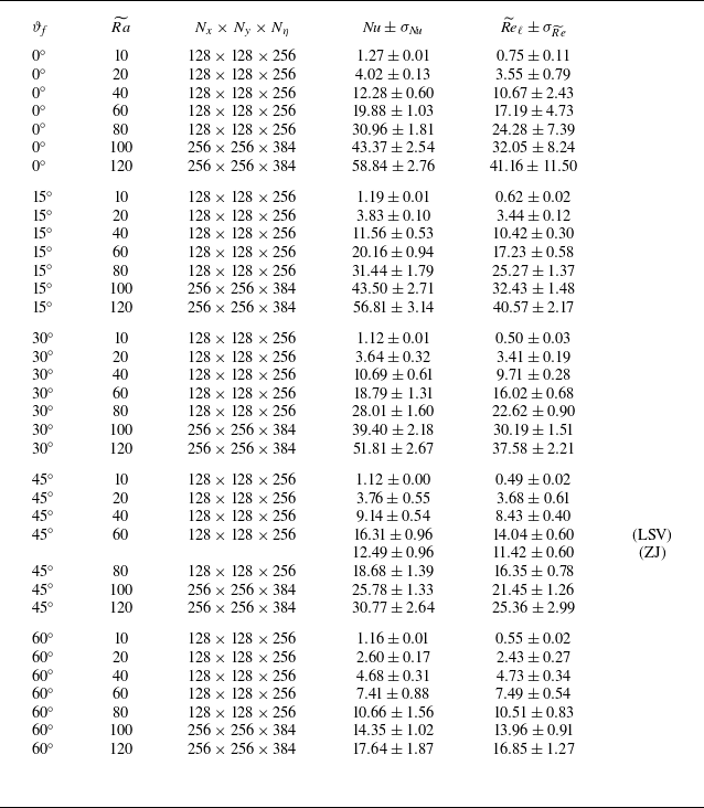
 σ=1
 Nu
 Re~ℓ

 θ
 Ra~=20
 ϑf=30∘
 y
 η
 Y
 Z
 10Lc×10Lc×1
 Ef1/3

 Ra~=120
 ϑf=60∘

 Ra~
 ϑf
 θ
 (x,y)
 Ra~
 ϑf
 Ra~

 η=0.5

 θ
 Ra~
 ϑf
 x
 y
 η
 (y,η)
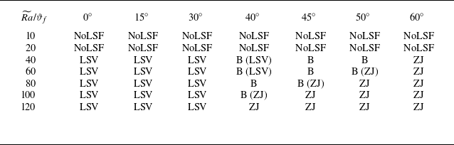
 Ra~
 ϑf

 Ψ′=Ψ−⟨Ψ⟩
 Ra~=120
 η=0.5
 ϑf=0∘
 (kx,ky)
 ky
 kx

 Ψ
 (x,y,η)
 Ra~
 ϑf
 ϑf

 Ra~=60
 ϑf=45∘
 ⟨u⟩rms=⟨u2⟩vol
 m≡(⟨u2⟩vol−⟨v~2⟩vol)/(⟨u2⟩vol+⟨v~2⟩vol)
 Nu−1≡σ⟨wθ⟩
 u=−∂yΨ
 v~=∂xΨ
 m
 m

 ⟨ζ⟩
 ⟨Ψ⟩
 Ra~=120
 ϑf∈{15∘,30∘,45∘,60∘}
 ϑf
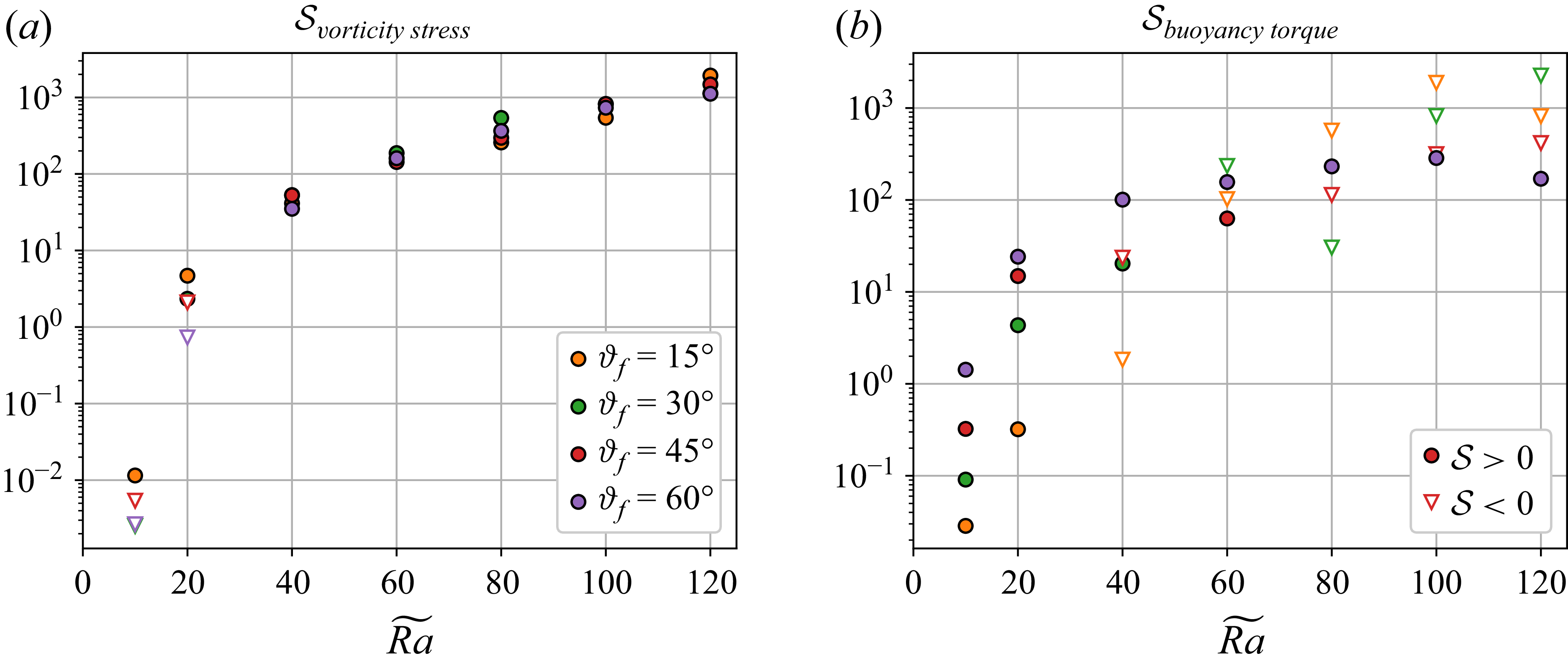
 Svorticitystress
 Sbuoyancytorque

 ⟨u′ζ′⟩rms
 ⟨v~′ζ′⟩rms
 Ra~
 ϑf
 η
 u=−∂yΨ
 v~=∂xΨ
 ζ=∇⊥′2Ψ
 ϑf=30∘
 60∘

 Ra~=120
 ϑf={15∘,30∘,45∘,60∘}
 p⊥≲10
 k⊥box=1
 Tk⊥
 k⊥
 p⊥
 k⊥

 Kbc(k⊥)
 Kbt(k⊥)
 Ra~=40
 Ra~=120
 ϑf

 Θ¯
 ϑf=0∘
 ϑf=60∘
 Ra~
 Ra~
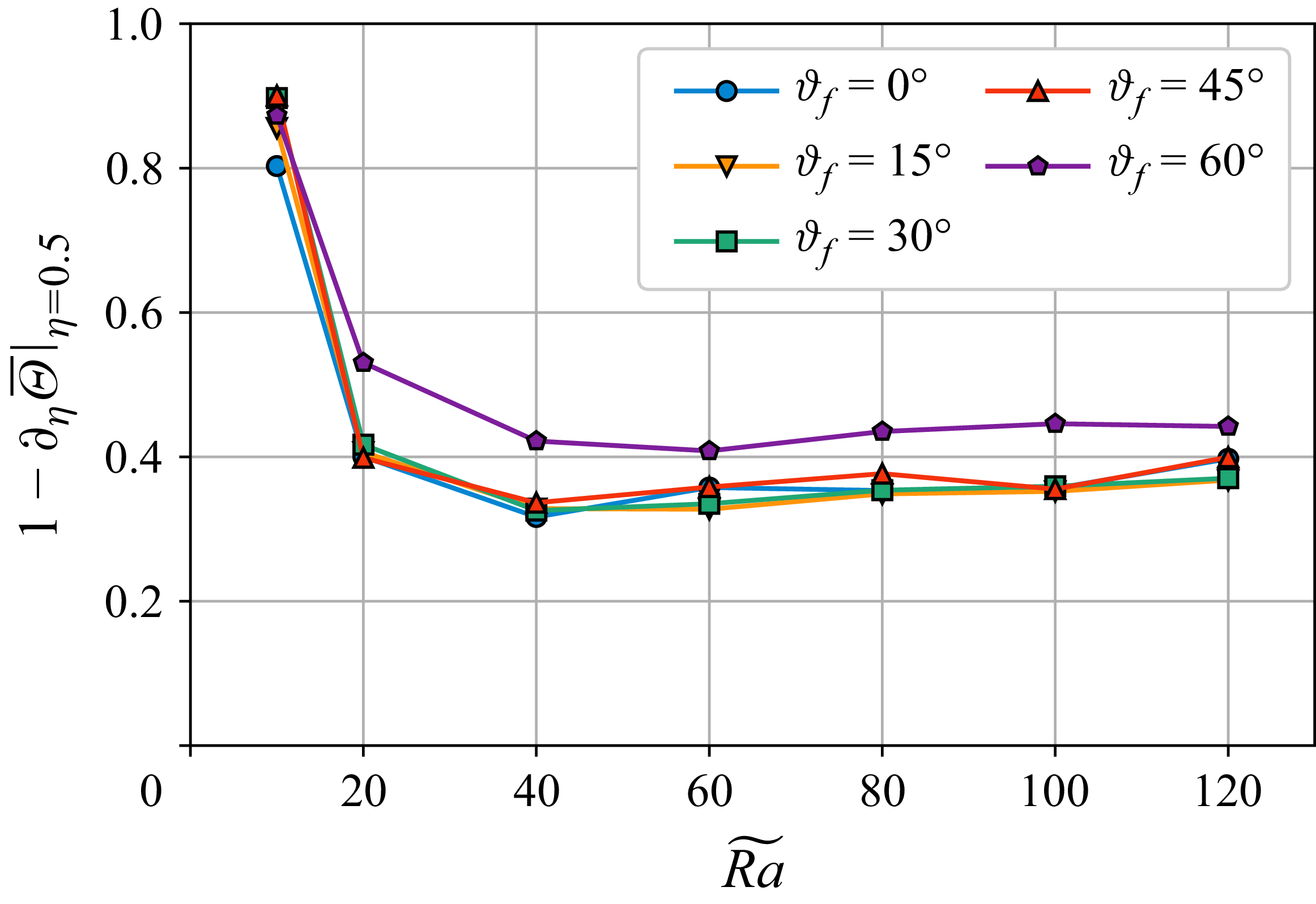
 ∂η(1−η+Θ¯)
 η=0.5
 Ra~
 ϑf
 Ra~

 Nu
 Re~ℓ
 Ra~
 ϑf
 Ra~3/2
 Ra~
 ϑf=45∘
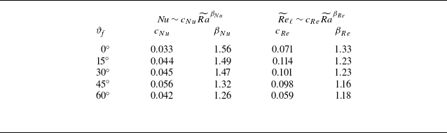
 Nu∼cNuRa~βNu
 Re~ℓ∼cReRa~βRe
 Ra~⩾60
 Nu∼Ra~3/2
 Re~ℓ∼Ra~1

 ϑf

 e^i
 e^i


 Open access

