

Marijuana is the most commonly used illicit drug among US adolescents, and use significantly increases with age. Although only 1% of US youth aged 12 to 13 reported past-month use in 2013, this number rose to 5.8% among youth aged 14 to 15, and to 14.2% among youth aged 16 to 17 (Substance Abuse and Mental Health Services Administration, 2014). By 12th grade, 21% of students reported having used marijuana in the past month, and almost half (44%) reported use in the past year (Johnston, O'Malley, Bachman, Schulenberg, & Miech, Reference Johnston, O'Malley, Bachman, Schulenberg and Miech2014). Although marijuana use among adolescents has remained stable over the past decade (Substance Abuse and Mental Health Services Administration, 2014), data from young adults (aged 19–28) indicate a steady increase in use since 2010 (Johnston et al., Reference Johnston, O'Malley, Bachman, Schulenberg and Miech2014), which the authors attribute to a decline in perceived harm of the drug as more states debate marijuana legalization. Legalization of marijuana for adults also raises concerns over increased availability of marijuana to younger adolescents, for whom marijuana use has been associated with school failure, mental health problems, and increased risk of addiction (Arseneault et al., Reference Arseneault, Cannon, Poulton, Murray, Caspi and Moffitt2002; Copeland, Rooke, & Swift, Reference Copeland, Rooke and Swift2013; Macleod et al., Reference Macleod, Oakes, Copello, Crome, Egger and Hickman2004; Silins et al., Reference Silins, Horwood, Patton, Fergusson, Olsson and Hutchinson2014). As marijuana legalization for adults spreads, a heightened focus on the factors driving marijuana etiology during adolescence will inform the development of adolescent preventive interventions.
Past research suggests that family and peer environmental factors, such as parent monitoring, affiliation with antisocial or deviant peers, and peer pressure, are influential predictors of substance use among adolescents (Hoeve et al., Reference Hoeve, Dubas, Eichelsheim, van der Laan, Smeenk and Gerris2009; Lac & Crano, Reference Lac and Crano2009; Reboussin, Hubbard, & Ialongo, Reference Reboussin, Hubbard and Ialongo2007; Steinberg, Fletcher, & Darling, Reference Steinberg, Fletcher and Darling1994). However, the effects of parents and peers are not static. As adolescents gain autonomy, studies have typically shown a decrease in the effect of family influence and an increase in the influence of peers (Cleveland, Feinberg, Bontempo, & Greenberg, Reference Cleveland, Feinberg, Bontempo and Greenberg2008; Ellickson, Tucker, Klein, & Saner, Reference Ellickson, Tucker, Klein and Saner2004; Tang & Orwin, Reference Tang and Orwin2009; Van Ryzin, Fosco, & Dishion, Reference Van Ryzin, Fosco and Dishion2012). In addition, theories of differential susceptibility (Belsky & Pluess, Reference Belsky and Pluess2009; Ellis, Boyce, Belsky, Bakermans-Kranenburg, & van IJzendoorn, Reference Ellis, Boyce, Belsky, Bakermans-Kranenburg and van IJzendoorn2011) recognize that individuals vary in their vulnerability or susceptibility to environmental influences and posit that there may be evolutionary and neurodevelopmental explanations to this variability (e.g., Wiebe et al., Reference Wiebe, Clark, De Jong, Chevalier, Espy and Wakschlag2015). In a recent update to the differential susceptibility work, Ellis et al. (Reference Ellis, Boyce, Belsky, Bakermans-Kranenburg and van IJzendoorn2011) outline fundamental features of differential susceptibility, including that susceptible individuals are more affected by both positive and negative environmental experiences and that variability in susceptibility is likely to change over development. One such vulnerability may be driven by dispositional characteristics, such as impulsivity, sensation seeking, and lack of constraint, which together form the construct behavioral disinhibition (Dever et al., Reference Dever, Schulenberg, Dworkin, O'Malley, Kloska and Bachman2012; Sher & Trull, Reference Sher and Trull1994; Slater, Reference Slater2003; Stephenson & Helme, Reference Stephenson and Helme2006). Studies have also begun to examine gender as a source of susceptibility, and whether the effect of parents and peers on marijuana use may be different for boys and girls (Choquet, Hassler, Morin, Falissard, & Chau, Reference Choquet, Hassler, Morin, Falissard and Chau2008; Fagan, Van Horn, Antaramian, & Hawkins, Reference Fagan, Van Horn, Antaramian and Hawkins2011; Parsai, Voisine, Marsiglia, Kulis, & Nieri, Reference Parsai, Voisine, Marsiglia, Kulis and Nieri2009). Few studies have examined whether the differences in the effects of parents and peers vary both over time and between these groups. The current study is the first to use a longitudinal approach to test these time-varying interactions with gender and behavioral disinhibition over the course of adolescence.
Theoretical Framework
The current work is based in two complementary theoretical approaches: the social development model (SDM; Catalano & Hawkins, Reference Catalano, Hawkins and Hawkins1996; Hawkins & Weis, Reference Hawkins and Weis1985) and the developmental psychopathology framework (Cicchetti & Rogosch, Reference Cicchetti and Rogosch2002; Cicchetti & Toth, Reference Cicchetti and Toth2009). The choice of environmental factors examined here is based here in the SDM, which organizes known risk and protective factors into causal mechanisms (Catalano & Hawkins, Reference Catalano, Hawkins and Hawkins1996). Rooted in previous psychological, sociological, and delinquency theories, the SDM is a developmentally informed model that outlines two parallel paths that lead to prosocial and antisocial outcomes. The SDM posits that reduced opportunities to engage in antisocial behavior (e.g., through parental monitoring of activities), coupled with rewards for prosocial actions, leads to adopting a prosocial value system and eventual engagement in more healthy behavior. The model also specifies a second parallel path, in which individuals have increased opportunities to bond with antisocial peers and adults (e.g., through limited family monitoring) and engage in antisocial actions, leading to the development of unhealthy behavior, such as substance use. The current work examines the protective effect of family management, operationalized as the combination of high monitoring and high prosocial rewards, on adolescent marijuana use. The presence of antisocial peers is hypothesized to present opportunities for antisocial behavior, combined with implicit social rewards that peers bring to one another.
Although the SDM recognizes the importance of both development and individual characteristics, the interplay of environmental and individual factors over time is well articulated by the developmental psychopathology integrative framework (Cicchetti & Rogosch, Reference Cicchetti and Rogosch2002; Cicchetti & Toth, Reference Cicchetti and Toth2009). The developmental psychopathology perspective emerged in response to a need to identify and prevent mental illness, and combines a focus on development with an emphasis on psychopathology (Masten, Reference Masten2006). The perspective highlights the interactive nature of multiple systems of development, including individual characteristics and environmental influences, and recognizes the importance of examining this interplay over time. We are guided by the developmental psychopathology perspective in our approach to examining how individual difference characteristics known to be related to substance use (gender and behavioral disinhibition) interact with environmental factors over the course of development. The perspective highlights that psychopathology needs to be examined in the context of development and would suggest that interactions are likely to be found at developmentally critical periods, such as during a transition or a sensitive period. This framework also highlights multifinality that occurs when risk and protective factors have divergent outcomes for different individuals or at different points in development. For example, boys might be more susceptible to peer pressure than girls. Conversely, equifinality occurs when individuals with different risk and protective factors in childhood exhibit similar outcomes later on. One example of equifinality might be that girls are more affected by family management during adolescence but that parental influence wanes for both boys and girls as they approach young adulthood. The potential for identifying critical periods when families and peers are particularly influential is important for the timing and delivery of interventions.
In sum, the SDM provides guidance in the selection of family management and antisocial peers as important environmental forces. Developmental psychopathology perspective leads us to examine the interaction between individual characteristics and these environmental factors. The current investigation connects these theoretical approaches to (a) examine the interplay of individual and environmental systems over the course of development and (b) focus on multifinality to explore differences in effects of families and peers over time by gender and level of behavioral disinhibition.
Differential Effects of Family Monitoring and Antisocial Peers on Marijuana Use by Gender and Behavioral Disinhibition
The links between family and peer factors and a range of adolescent outcomes have been widely demonstrated. Family management, or family monitoring, has been shown to be particularly associated with reduced substance use, including marijuana, among adolescents (Hoeve et al., Reference Hoeve, Dubas, Eichelsheim, van der Laan, Smeenk and Gerris2009; Lac & Crano, Reference Lac and Crano2009; Shillington et al., Reference Shillington, Lehman, Clapp, Hovell, Sipan and Blumberg2005; Steinberg et al., Reference Steinberg, Fletcher and Darling1994). This protective effect of family management and monitoring on marijuana use, in particular, has been shown for younger and older adolescents (Chilcoat & Anthony, Reference Chilcoat and Anthony1996; DiClemente et al., Reference DiClemente, Wingood, Crosby, Sionean, Cobb and Harrington2001; Hayatbakhsh et al., Reference Hayatbakhsh, Mamun, Najman, O'Callaghan, Bor and Alati2008; Lac & Crano, Reference Lac and Crano2009), in nationally representative (Dever et al., Reference Dever, Schulenberg, Dworkin, O'Malley, Kloska and Bachman2012; Martins, Storr, Alexandre, & Chilcoat, Reference Martins, Storr, Alexandre and Chilcoat2008; Rodgers-Farmer, Reference Rodgers-Farmer2000) and community samples (Dishion, Nelson, & Kavanagh, Reference Dishion, Nelson and Kavanagh2003; Hill et al., Reference Hill, Hawkins, Bailey, Catalano, Abbott and Shapiro2010; Kosterman, Hawkins, Guo, Catalano, & Abbott, Reference Kosterman, Hawkins, Guo, Catalano and Abbott2000), and for a range of socioeconomic and ethnic groups (Bohnert, Anthony, & Breslau, Reference Bohnert, Anthony and Breslau2012; Griffin, Botvin, Scheier, Diaz, & Miller, Reference Griffin, Botvin, Scheier, Diaz and Miller2000; Lac & Crano, Reference Lac and Crano2009; Moon, Blakey, Boyas, Horton, & Kim, Reference Moon, Blakey, Boyas, Horton and Kim2014; Yabiku et al., Reference Yabiku, Marsiglia, Kulis, Parsai, Becerra and Del-Colle2010). In a similar vein, the negative association between drug-using or antisocial peers and substance use has also been well established. Associating with antisocial or drug-using peers has been linked to marijuana use in multiple samples and in diverse populations of adolescents (Dishion & Owen, Reference Dishion and Owen2002; Donohew et al., Reference Donohew, Hoyle, Clayton, Skinner, Colon and Rice1999; Hampson, Andrews, & Barckley, Reference Hampson, Andrews and Barckley2008; Kosterman et al., Reference Kosterman, Hawkins, Guo, Catalano and Abbott2000; Moon et al., Reference Moon, Blakey, Boyas, Horton and Kim2014; Rodgers-Farmer, Reference Rodgers-Farmer2000; Steinberg et al., Reference Steinberg, Fletcher and Darling1994; Van Ryzin et al., Reference Van Ryzin, Fosco and Dishion2012; Yanovitzky, Reference Yanovitzky2005). The main effects of gender and behavioral disinhibition on substance use are similarly robust and well documented (Donohew et al., Reference Donohew, Hoyle, Clayton, Skinner, Colon and Rice1999; Kopstein, Crum, Celentano, & Martin, Reference Kopstein, Crum, Celentano and Martin2001; Newcomb & McGee, Reference Newcomb and McGee1991; Sargent, Tanski, Stoolmiller, & Hanewinkel, Reference Sargent, Tanski, Stoolmiller and Hanewinkel2010; Teichman, Barnea, & Ravav, Reference Teichman, Barnea and Ravav1989).
Researchers also have investigated interactions between monitoring and antisocial peers on one hand and gender and behavioral disinhibition on the other hand, based on the hypothesis that boys or highly disinhibited youth may be more or less responsive to environmental influence than girls or less disinhibited youth. Among studies that have examined differential influence of family monitoring and antisocial peers by gender, no consistent pattern of results emerged. For example, two studies of European (McArdle et al., Reference McArdle, Wiegersma, Gilvarry, Kolte, McCarthy and Fitzgerald2002) and US (Griffin et al., Reference Griffin, Botvin, Scheier, Diaz and Miller2000) adolescents found that family monitoring and supervision were more related to boys’ than to girls’ alcohol use. Other investigations and a recent meta-analysis of 17 studies found that family influence had greater effects on curbing girls’ marijuana use (e.g., Choquet et al., Reference Choquet, Hassler, Morin, Falissard and Chau2008; Lac & Crano, Reference Lac and Crano2009). Still, others have reported no gender difference in the effect of family monitoring on substance use (Chen & Jacobson, Reference Chen and Jacobson2013; Fagan et al., Reference Fagan, Van Horn, Antaramian and Hawkins2011). Studies of peer effects on substance use have found similar discrepancies in whether boys or girls are more susceptible to peer influence. For example, in a study of Mexican American adolescents, perception of peer use and peer norms was more related to boys’ than to girls’ marijuana use (Parsai et al., Reference Parsai, Voisine, Marsiglia, Kulis and Nieri2009), but another study found that the association between antisocial peers and alcohol use was equally strong for boys and for girls (Simons-Morton, Haynie, Crump, Eitel, & Saylor, Reference Simons-Morton, Haynie, Crump, Eitel and Saylor2001).
Few studies to date have examined whether the link between family monitoring and substance use varies by behavioral disinhibition, and the results are inconsistent. One study found that sixth to eighth graders with higher behavioral disinhibition reported less intent to use marijuana when family management was high (Stephenson & Helme, Reference Stephenson and Helme2006), whereas another investigation found no difference in marijuana dependence by adolescent parental monitoring and levels of behavioral disinhibition among college students (Kaynak et al., Reference Kaynak, Meyers, Caldeira, Vincent, Winters and Arria2013). Studies of differential influence of peers by behavioral disinhibition, however, suggest a clearer story. Most studies found that adolescents who reported high behavioral disinhibition and also had antisocial peers had greater rates of substance use than less disinhibited youth (Epstein & Botvin, Reference Epstein and Botvin2002; Knyazev, Slobodskaya, Kharchenko, & Wilson, Reference Knyazev, Slobodskaya, Kharchenko and Wilson2004; Slater, Reference Slater2003). We found no studies where the effect of peers was greater for individuals with lower behavioral disinhibition.
Change in Risk and Protective Factors Over the Course of Adolescence
Throughout the course of adolescence, young people spend increasing amounts of time away from home, most often in the company of their peers (Furman & Buhrmester, Reference Furman and Buhrmester1992), and less time under parental supervision. Thus, it is often believed that family monitoring decreases both in amount and in effectiveness to reduce problem behavior as young people move toward legal adulthood (Cleveland et al., Reference Cleveland, Feinberg, Bontempo and Greenberg2008; Cleveland, Feinberg, & Jones, Reference Cleveland, Feinberg and Jones2012). At the same time, as peers become more salient during the transition from childhood to adolescence, their influence is thought to increase as well (Van Ryzin et al., Reference Van Ryzin, Fosco and Dishion2012).
Studies examining the effects of parents and peers over time generally confirm the decline of parent influence (Jang, Reference Jang2002; Kelly et al., Reference Kelly, Toumbourou, O'Flaherty, Patton, Homel and Connor2011; Reboussin et al., Reference Reboussin, Hubbard and Ialongo2007; Seydlitz, Reference Seydlitz1991; Van Ryzin et al., Reference Van Ryzin, Fosco and Dishion2012), although the results are not always consistent. For example, in a large cross-sectional sample from the Pennsylvania Youth Risk Study, Cleveland et al. (2012) found that the relationship between family risk factors and alcohol use declined from 6th to 12th grade, although the relationship with marijuana use from 8th to 12th grade remained steady. However, another large study of high school students in 24 US communities found no change in the relationship between family factors and substance use, even though the amount of family monitoring declined from 8th to 12th grade (Fagan et al., Reference Fagan, Van Horn, Antaramian and Hawkins2011). The declining levels, rather than effectiveness, of family monitoring may provide a clue as to why, at a population level, the influence of the family appears to wane as children mature. In contradiction, however, a meta-analysis of over 350 studies found that the effect of family on drug use increases with age (Allen, Donohue, Griffin, Ryan, & Turner, Reference Allen, Donohue, Griffin, Ryan and Turner2003).
A review of the literature examining the change in the strength of peer influence on substance use over the course of adolescence did not unilaterally support the notion that peers become more influential. Although some studies (Cleveland et al., Reference Cleveland, Feinberg, Bontempo and Greenberg2008; Jang, Reference Jang2002; Van Ryzin et al., Reference Van Ryzin, Fosco and Dishion2012), including a meta-analysis (Allen et al., Reference Allen, Donohue, Griffin, Ryan and Turner2003), found that peer influence increased over time, several notable exceptions reported that peer influence declined (Abadi, Shamblen, Thompson, Collins, & Johnson, Reference Abadi, Shamblen, Thompson, Collins and Johnson2011; Fergusson, Swain-Campbell, & Horwood, Reference Fergusson, Swain-Campbell and Horwood2002). In addition, two separate longitudinal studies reported that the effect of delinquent peers on substance use followed a curvilinear trend such that peer influence peaked in middle to late adolescence and then plateaued (Cleveland et al., Reference Cleveland, Feinberg and Jones2012; Jang, Reference Jang2002).
Adding to the complexity is the possibility that the effects of peers and parents on substance use over time may follow a different trend for different groups. For example, Dever et al. (Reference Dever, Schulenberg, Dworkin, O'Malley, Kloska and Bachman2012) found that the association between family management and drug use varied by gender and level of behavioral disinhibition, as well as over time. Because the effect sizes of risk and protective factors vary over the course of development, it is likely that the interactions of those effects with gender and behavioral disinhibition are also specific to certain developmental periods. It could be that some interactions are most evident during younger or older adolescence, or even during periods of change, such as the transition to middle school or high school. An underlying curvilinear pattern to the influence of environmental factors on substance use could explain the inconsistency in results from studies reporting an effect at a single point in time from different parts of the effect curve. Methods that are able to model nonlinear change in effects and can test interactions longitudinally can shine a light on this complexity.
The current study bridges several literatures that investigate risk and protective factors related to adolescent marijuana use. Specifically, the current work uses an innovative longitudinal method to examine nonlinear change in the association between family management and antisocial peers and marijuana use. Analyses using time-varying effect modeling (TVEM) assess the change in the associations throughout adolescence and examine the degree to which they are moderated by gender and behavioral disinhibition. Specifically, the study has three research aims:
-
1. to examine changes in the strength of the association (main effects) between adolescent marijuana use and four predictors: family management, antisocial peers, gender, and behavioral disinhibition;
-
2. to test time-varying interactions between family management and gender and behavioral disinhibition in predicting adolescent marijuana use; and
-
3. to test time-varying interactions between antisocial peers and gender and behavioral disinhibition in predicting adolescent marijuana use.
Methods
Participants
Participants were drawn from the Raising Healthy Children project, a longitudinal study of students recruited from public elementary schools in a suburban Pacific Northwest school district. The project was designed to study the etiology of problem behaviors and to test a randomized preventive intervention (for detailed descriptions of the Raising Healthy Children intervention, see Catalano et al., Reference Catalano, Mazza, Harachi, Abbott, Haggerty and Fleming2003). Two cohorts of families with students in first and second grade in the project schools were invited to participate in the study. Active consent was obtained from 76% of eligible families, and 1,040 students were enrolled in 1993 and 1994. Parental consent and children's assent (until age 18 when child consent was required) were obtained at each wave. All procedures were approved by the University of Washington's Human Subjects Review Committee. Participant surveys were administered at least annually in the spring until 2011 when participants were 24 and 25 years old (younger and older cohort, respectively). Parent and teacher data were collected annually through ages 14/15 (younger/older cohort) for teachers and through age 18 for parents. The current study used participant data from ages 10 through 18 (Grade 12) with 8,320 available person-occasions. Retention was high, with >85% of participants retained from study inception to the last time point.
Of this original sample, 53% were male and 38% were low income, defined by eligibility for the National School Lunch Program or family receipt of food stamps or Temporary Aid for Needy Families in elementary school. The ethnic composition of the sample of was 75% White, 7% Asian American or Pacific Islander, 4% African American, 2% Native American, and 12% mixed ethnicity. Half (54%) of the sample was randomly assigned to receive a preventive intervention during Grades 1–12. Previous examinations of the differences between control and intervention groups did not find differences in outcome behaviors, including marijuana use (Brown, Catalano, Fleming, Haggerty, & Abbott, Reference Brown, Catalano, Fleming, Haggerty and Abbott2005).
Measures
Marijuana use was based on participant self-reports from ages 11 to 19. At age 11/12 participants were asked if they ever used marijuana; starting at age 12/13, participants reported past-month use. Marijuana use was coded at each age as 1 if participants indicated any use and 0 if they indicated no use over the specified period. Because only 3% of the sample reported using any marijuana at age 11/12, we felt comfortable combining the “ever” measure for one time point with past-month measures in the rest of the analyses.
Family management was assessed using a five-item scale based on participant self-reports from ages 10 to 19. Each year, participants were asked about parents’ practices around monitoring, discipline, and rewards. Examples include When you are not home, do your parents know where you are and who you are with? Are the rules in your family clear? Does your mom or dad notice when you've helped out at home? Responses were scored on a 4-point scale (NO!, no, yes, YES!). Items were averaged at each age and then standardized (average Cronbach α = 0.71). Family management variables were treated as time-varying predictors and were lagged 1 year. For example, age 10 family management was used to predict age 11 marijuana use.
Antisocial peer behavior was assessed using a three-item scale based on participant self-reports from ages 11 to 19. Each year, participants were asked How many of your 10 best friends get into fights? How many of your 10 best friends skip school or class? and How many of your 10 best friends get in trouble with their teacher? Responses for each item were scored on a 5-point scale (1 = none to 5 = a lot), and scores were averaged at each age and then standardized (average Cronbach α = 0.72). Similar to family management, antisocial peers variables were treated as time-varying predictors and were lagged 1 year.
Behavioral disinhibition was assessed through a three-item scale assessing impulsivity, reward orientation, and sensation seeking based on participant self-reports from ages 14 to 19. Each year, participants reported how often in the past year they have done: crazy things even if they were a little dangerous, something dangerous because someone dared you to do it, and what feels good no matter what? Responses for each item were scored on a 6-point scale (1 = never to 6 = once a week or more) and averaged across all ages, then standardized (average Cronbach α = 0.66).
Gender was self-reported (1 = male, 0 = female).
Analysis
TVEM
TVEM in SAS was used to examine the effects of family management and antisocial peers on marijuana use across adolescence. TVEM is based in spline regression and estimates an association that is allowed to vary as a nonparametric function of time. That is, the TVEM method makes no assumptions about change as being parametric (linear, quadratic, etc.). Instead, the effect size curve is based on the strength of the association at each point in development and is assumed to be smooth at the population level (Tan, Shiyko, Li, Li, & Dierker, Reference Tan, Shiyko, Li, Li and Dierker2012). TVEM has been effectively used to model ecological momentary assessment data (Lanza, Vasilenko, Liu, Li, & Piper, Reference Lanza, Vasilenko, Liu, Li and Piper2014) as well as data from longitudinal panels (Vasilenko & Lanza, Reference Vasilenko and Lanza2014). TVEM macros are designed to work with outcomes that are normally distributed, binary, or Poisson. Macros are available to download from http://www.methodology.psu.edu (Li, Tan, Huang, Wagner, & Yang, Reference Li, Tan, Huang, Wagner and Yang2014). TVEM effects can be modeled as both time fixed and time varying; that is, a time-varying effect can be estimated for a static predictor like gender or a predictor that changes over time, such as family management.
TVEM analyses were based on participants’ exact age (as opposed to wave) at the time of the interview that was calculated from birth dates and interview dates. Participant age ranged from 10.18 to 20.36 years, but data was sparse at the upper and lower ends of the age distribution. For analyses involving family management, participants younger than 11 and older than 19 were excluded, reducing the person-occasions from 8,320 to 7,754. Because antisocial peer variables were only available starting at age 11 and variables were lagged 1 year, we limited those analyses to ages 12 to 19, reducing person-occasions to 7,045. This created a continuous distribution of data over the target age span (for further detail on the use of TVEM for longitudinal data, see Vasilenko & Lanza, Reference Vasilenko and Lanza2014). In keeping with the TVEM language we use the word “effect” here to refer to the strength of the association rather than a causal inference. Because of its nonparametric nature, TVEM does not formally estimate whether the effect magnitude is larger or smaller at different points in development; however, nonoverlapping confidence intervals are indicators of significant difference in the association.
Research aims
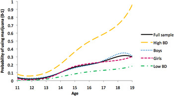
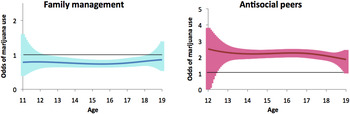
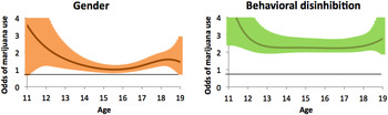
In response to research aim 1, we first show the probability of marijuana use in the past month by gender and behavioral disinhibition (Figure 1). Time-varying main effects (without an interaction term) of family management (Model 1) and antisocial peers (Model 2) are shown in Figure 2, and time-varying main effects of gender (Model 3) and behavioral disinhibition (Model 4) are shown in Figure 3.
(Color online) Probability of marijuana use by gender and behavioral disinhibition.

(Color online) The time-varying main effect of family management (lagged 1 year) and antisocial peers (lagged 1 year) on marijuana use, with 95% confidence intervals. Model 1 is presented on the left-hand side; Model 2 is on the right. Models are adjusted for ethnicity, childhood socioeconomic status, cohort, and intervention status.

(Color online) The time-varying main effect of gender and behavioral disinhibition on marijuana use, with 95% confidence intervals. Model 3 is presented on the left-hand side; Model 4 is on the right. Models are adjusted for ethnicity, childhood socioeconomic status, cohort, and intervention status.

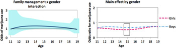
Next, to address research aim 2, we tested two time-varying interaction models with family management: Model 5, Family Management × Gender (Figure 4), and Model 6, Family Management × Behavioral Disinhibition (Figure 5). In a similar vein, research aim 3 was addressed in Model 7, Antisocial Peers × Gender (Figure 6), and Model 8, Antisocial Peers × Behavioral Disinhibition (Figure 7; Although the full range of behavioral disinhibition was tested in the interaction models, for illustration purposes in Figures 6 and 7 we show odds ratios for the participants in the top 33% of the distribution of behavioral disinhibition v. those in the bottom two-thirds). On the left sides of Figures 4–7, we include the time-varying interaction effects with 95% confidence intervals, which were significant in the regions where the confidence interval does not cross the value of 1. Adjacent on the right, we plot the main effects by the moderator (gender or by behavioral disinhibition) to illustrate the interaction term. These illustrations were estimated by stratifying the sample by gender or the top tertile of the distribution of behavioral disinhibition and estimating a main effects only model with control variables. This approach is laid out in the TVEM macro guide (Li et al., Reference Li, Tan, Huang, Wagner and Yang2014).
(Color online) Time-varying main effect of family management on marijuana use, by gender (Family Management × Gender interaction). Time-varying interaction of Model 5 is plotted on the left. The difference in the main effects is illustrated on the right. The area inside the box represents time span during which the gender interaction is significant at p < .05. Models are adjusted for ethnicity, childhood socioeconomic status, cohort, and intervention status.

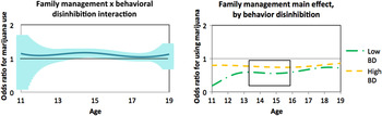
(Color online) Time-varying main effect of family management on marijuana use, by behavioral disinhibition (Family Management × Behavioral Disinhibition interaction). Time-varying interaction of Model 6 is plotted on the left. The difference in the main effects is illustrated on the right. The area inside the box represents time span during which the behavioral disinhibition interaction is significant at p < .05. Models are adjusted for gender, ethnicity, childhood socioeconomic status, cohort, and intervention status.

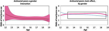
(Color online) Time-varying main effect of antisocial peers on marijuana use, by gender (Antisocial Peers × Gender interaction). Time-varying interaction of Model 7 is plotted on the left. The difference in the main effects is illustrated on the right. The area inside the box represents time span during which the gender interaction is significant at p < .05. Models are adjusted for ethnicity, childhood socioeconomic status, cohort, and intervention status.

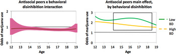
(Color online) Time-varying main effect of antisocial peers on marijuana use, by behavioral disinhibition (Antisocial Peers × Behavioral Disinhibition interaction). Time-varying interaction of Model 8 is plotted on the left. The difference in the main effects is illustrated on the right. The area inside the box represents time span during which the behavioral disinhibition interaction is significant at p < .05. Models are adjusted for gender, ethnicity, childhood socioeconomic status, cohort, and intervention status.

Controls
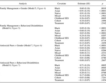
All models included time-fixed control variables: ethnicity (dummy coded), childhood socioeconomic status, sample cohort, and treatment condition. Time-fixed effects of the controls for Models 5–8 are shown in Table 1. In addition, models testing group differences by behavioral disinhibition (Models 6 and 8) included gender, which was entered as a time-varying variable. For example, Model 6, estimating the relationship between family management and marijuana use by behavioral disinhibition (Figure 5), included family management, behavioral disinhibition, their interaction term (Family Management × Behavioral Disinhibition), and gender as time-varying predictors; ethnicity, childhood socioeconomic status, and cohort were included as time fixed.
Time-fixed coefficient estimates

Note: The ethnicity referent was White. SES, Socioeconomic status.
Results
Research aim 1: Main effects
Figure 1 shows the rate of marijuana use from ages 12 to 19 for the full sample, and separately by gender and levels of behavioral disinhibition (top third vs. bottom two-thirds). In the full sample, about 30% of participants reported past-month marijuana use at age 19. Boys generally reported slightly higher levels of marijuana use than girls. Among those in the top third of the behavioral disinhibition distribution, past-month marijuana use by age 19 was about 90%, whereas among those in the bottom two-thirds it was about 20%.
Models 1 and 2, showing the main effects of family management and antisocial peers (each lagged by 1 year) on marijuana use, are shown in Figure 2. The y axis presents the odds of past-month marijuana use for each standard deviation of family management or antisocial peers. The solid lines represent estimates of the strength of the association between family management and marijuana use (left side) and antisocial peers and marijuana use (right side). The 95% confidence interval is shown as the shaded area around the solid line. The horizontal line at the value of 1 shows the significance for odds ratios; when the 95% confidence interval crosses the line, the significance of the estimate falls below p = .05.
Model 1 shows that odds ratios of marijuana use were <1, indicating that family management was significantly associated with lower odds of marijuana use from ages 12 to 19. The effect was significant (confidence interval values did not cross 1) from ages 12.3 to 18.2. Effect sizes for the full sample ranged from an odds ratio of 0.73 at age 15.5 to an odds ratio of 0.86 at age 19. This pattern suggests a possible decline in the protective power of family management across adolescence. The main effect of antisocial peers (Model 2), presented on the right-hand side of Figure 2, shows values of >1, suggesting that the presence of antisocial peers in the previous year was associated with a significant increase in the odds of marijuana use from ages 12.5 to 19. The odds of marijuana use varied from approximately 2.5 at age 12 to 1.85 at age 19, suggesting a decrease in the effect of peers over the adolescent period.
Figure 3 shows the time-varying main effect of the moderators: (male) gender (Model 3) and behavioral disinhibition (Model 4). On the left-hand side, the main effect of gender had odds ratios of >1, revealing that being male was associated with significantly greater odds of marijuana use than being female. This difference was significant in early and late adolescence (approximately < age 13.3 and > age 17). The gender odds varied from just under 3 at age 11.5 to 1.58 at age 15; that is, at age 11.5, the odds of marijuana use for a boy were three times as high as for a girl, whereas the difference in odds was closer to 0.01–0.05 and not significantly different by gender at age 15. The right side of Figure 3 shows the main effect of behavioral disinhibition on marijuana use, which was relatively stable and significant throughout adolescence. With odds ratios >1, greater behavioral disinhibition predicted higher odds of marijuana use, with one standard deviation change in the behavioral disinhibition measure increasing the odds of using marijuana 2.8 times at age 12 and approximately 2.2 times at age 15.
Research aim 2: Interactions with family management
We tested whether family management had a differential effect on marijuana use for girls versus boys (Model 5) and for adolescents with high versus low behavioral disinhibition (Model 6). Figure 4 shows the time-varying interaction for Model 5, and then plots the main effects of family management for boys and girls separately. The left side shows the time-varying interaction term, which is significant in the region where the confidence interval does not cross the value of 1. This region is demonstrated on the right side by a black box. The gender interaction was significant for a period of adolescence consistent with the transition to high school (approximate ages 14.6–15.1). That is, the significant main effect shows that consistent family management was associated with a lower likelihood of marijuana use for both girls and boys. However, during the transition to high school, the significant interaction suggests that this association was stronger for girls than for boys. On the right side of Figure 4, this can be observed as the curve for boys being closer to the reference line at 1 (i.e., weaker effect of family management for boys). The interaction value (exponentiated) was around 1.25 at age 15, meaning that the odds of girls using marijuana was 25% lower than the odds of boys using marijuana at average levels of family management.
Next, Model 6 tested whether the effect of family management was different for adolescents with high versus lower levels of behavioral disinhibition (controlling for the time-varying effect of gender). The interaction shown on the left-hand side of Figure 5 was significant at approximately ages 13.4 to 16, roughly the same period of the transition to high school during which the effect of family management differed by gender. The right-hand side of Figure 5 plots the effect of family management on marijuana use separately by levels of behavioral disinhibition, showing that the effect was greater for adolescents with lower levels of behavioral disinhibition than more disinhibited adolescents. The exponentiated interaction value was about 1.15 throughout the significant region, corresponding to about 15% higher odds of marijuana use for youth with lower behavioral disinhibition. However, for all youth, family management had a consistent protective main effect. A three-way interaction with family management, gender, and behavioral disinhibition was also tested and showed a small region of significance between ages 11 and 13.
Research aim 3: Interactions with antisocial peers
We followed a parallel process to test interactions with antisocial peers by gender and behavioral disinhibition. Figure 6 shows the interaction between antisocial peers and gender (Model 7). The interaction was significant from ages 12.1 to 18.4 (Figure 6, left side). The magnitude of the interaction effect ranged from over 2 at age 12 to 1.30 at age 18. The right side of Figure 6 shows that the presence of antisocial peers was associated with greater (30%–200%) odds of marijuana use for girls than for boys during most of adolescence.
Figure 7 presents the interaction of antisocial peers with behavioral disinhibition (Model 8). Similar to family management, results on the left side of Figure 7 show significant interactions in mid dleadolescence (around age 14.5) and up to age 18.4. The right side of Figure 7 shows that adolescents with lower levels of behavioral disinhibition were more susceptible to the influence of antisocial peers; the interaction values ranged from 0.84 to 0.89. Thus, antisocial peers had 12% to 19% more influence on marijuana use for adolescents with lower levels of behavioral disinhibition than for more disinhibited youth (although, for all youth, it was associated with generally more marijuana use). A three-way interaction with gender and behavioral disinhibition was not significant at any time.
Control variables
Table 1 shows estimates for time-fixed covariates for Models 5–8. In all models, identifying as Black or Native American was associated with greater odds of marijuana use, compared to being White. Identifying as Asian reduced the odds in all models. Mixed ethnicity was significantly associated with higher odds of marijuana use only in Model 6 (Family Management × Behavioral Disinhibition). Childhood socioeconomic status was related to greater odds of marijuana use in all analyses except in Model 7 (Antisocial Peers × Gender). Finally, cohort and intervention condition were unrelated to marijuana use in any of the four analyses.
Discussion
The current study aimed to clarify questions related to changes in the strength of association between known risk and protective factors and marijuana use over the course of adolescence. Previous investigations have yielded few consistent findings about whether the strength of family and peer predictors increases or decreases over time, and whether some youth are more susceptible to their influence. Some of the confusion is likely due to differential age sampling in different studies, to the fact that changes in the size of predictive effects may be nonlinear (e.g., Cleveland et al., Reference Cleveland, Feinberg and Jones2012), and to limited availability of methodologies that test changes in effect size over time. In this study we attempted to address these limitations by using TVEM, which allowed us to fully utilize the longitudinal data from the Raising Healthy Children study and to test interactions between individual and environmental factors throughout adolescence.
The results from this investigation show that family management had a consistent negative association with marijuana use. For the entirety of the developmental period examined in the current analysis (ages 12–19), we observed that good family management was associated with reduced likelihood of marijuana use for all adolescents. This association remained unchanged until late adolescence, around the time when youth tend to leave the parental home. However, some multifinality in the effect of family management was observed: girls and adolescents with lower levels of behavioral disinhibition may have benefitted more from good family management than boys and more disinhibited adolescents, and these differences were most pronounced during the transition to high school. It is important to note, however, that family management was also associated with significantly lower odds of marijuana use for boys and less inhibited youth across adolescence, even if the size of the effect was slightly smaller. Analyses also showed that exposure to antisocial peers was associated with higher odds of using marijuana for the same developmental period (ages 12–19). Peer effects were also robustly related to marijuana use and were relatively stable over time. Here, multifinality by gender and behavioral disinhibition was also observed, but the timing was different than for family management. Association with antisocial peers was linked to higher odds of marijuana use, and this relationship was stronger for girls than for boys in the late teenage years. The relationship between antisocial peers and marijuana use was also stronger for youth with lower levels of behavioral disinhibition; this effect was significant throughout middle and late adolescence.
Comparison with previous findings
Our main findings are consistent with prior studies that have shown both family management and exposure to antisocial peers to be related to adolescent substance use. Prior research examining the interaction of antisocial peers and family management with gender has produced inconsistent results as to which gender is more susceptible to environmental influences (Choquet et al., Reference Choquet, Hassler, Morin, Falissard and Chau2008; McArdle et al., Reference McArdle, Wiegersma, Gilvarry, Kolte, McCarthy and Fitzgerald2002; Parsai et al., Reference Parsai, Voisine, Marsiglia, Kulis and Nieri2009; Simons-Morton et al., Reference Simons-Morton, Haynie, Crump, Eitel and Saylor2001). In the current study, we found that the association of family management with antisocial peers was stronger for girls than for boys, but only during the transition to high school. Some researchers have raised questions about the role that child disclosure plays in parents’ knowledge (a part of parental management) about the child's whereabouts. For example, Eaton, Krueger, Johnson, McGue, and Iacono (Reference Eaton, Krueger, Johnson, McGue and Iacono2009) reported associations between gender, child personality traits, and disclosure, suggesting that some children are more likely to facilitate monitoring by volunteering information. Girls with greater harm avoidance (lower behavior disinhibition) tendencies disclosed more than more disinhibited girls. This is a pattern of results generally consistent with our findings. Families are believed to monitor girls more closely than boys as part of a sexual double standard that makes it more acceptable for boys to engage in some antisocial behaviors (Smetana & Daddis, Reference Smetana and Daddis2002; Tucker, McHale, & Crouter, Reference Tucker, McHale and Crouter2003; Varner & Mandara, Reference Varner and Mandara2014). It is possible that parents expect greater disclosure from girls and provide greater sanctions for girls’ misbehavior, thereby increasing the likelihood of disclosure.
In a similar vein, gender differences in peer influence may be explained by gender-based substance use norms (Schulenberg, Reference Schulenberg1999; Simons-Morton et al., Reference Simons-Morton, Haynie, Crump, Eitel and Saylor2001). Boys, for whom marijuana use is more normative than for girls, may be less dependent on peer influence to engage in marijuana use. Some of the inconsistency in gender effects in the literature may be due to the relatively low prevalence of girls reporting antisocial peers compared to boys in some samples (Mears, Ploeger, & Warr, Reference Mears, Ploeger and Warr1998; Svensson, Reference Svensson2004), such that girls who have antisocial peers are relative outliers, and thus may be more likely to use marijuana.
The current study also found that the association between family management and antisocial peers and marijuana use differed by behavioral disinhibition and that less disinhibited youth were more susceptible to outside influence. This is interesting given that some advocates of selective intervention recommend identifying and selecting for intervention youths at higher risk (see Bröning et al., Reference Bröning, Kumpfer, Kruse, Sack, Schaunig-Busch and Ruths2012), when in this case, the lower risk youth were most responsive to these environmental experiences. These findings are not without precedent. Several studies have found that antisocial peers had the strongest effect on youth who are less impulsive and have higher self-control (Meldrum, Miller, & Flexon, Reference Meldrum, Miller and Flexon2013; Thomas & McGloin, Reference Thomas and McGloin2013; Vitulano, Fite, & Rathert, Reference Vitulano, Fite and Rathert2010). It is possible that more disinhibited youth choose peers who, like them, are more likely to engage in substance use. Similar to the case of boys versus girls, for disinhibited youth, marijuana use would be driven more by their own sensation seeking than by peer influence, whereas less disinhibited youth might start using marijuana only in the presence of antisocial peers. Another possible explanation, as put forth by Thomas and McGloin (Reference Thomas and McGloin2013), is that high- and low-impulsive youth may be differentially susceptible to different types of peer influence. They posit that low-impulsive youth may be more susceptible to normative peer influence (shared values and behavior reinforcement), whereas high-impulsive youth may be most susceptible to situational peer influences (opportunities that arise during unstructured or unsupervised time with peers). This might partially explain why these contradictory results have emerged.
Our finding that family management had a greater effect for less disinhibited youth deviates from the few studies that have examined this interaction (Chen & Jacobson, Reference Chen and Jacobson2013; Hill et al., Reference Hill, Hawkins, Bailey, Catalano, Abbott and Shapiro2010; Kaynak et al., Reference Kaynak, Meyers, Caldeira, Vincent, Winters and Arria2013; Stephenson & Helme, Reference Stephenson and Helme2006). It may be that traditional family management approaches are not as effective for more disinhibited youth because these youth are less likely to voluntarily disclose to parents or to consider the consequences of their actions. This might suggest the need for more targeted parenting techniques for families with more disinhibited youth in addition to consistent family management. For example, programs teaching interpersonal skills to temper behavioral disinhibition also seem promising (e.g., Conrod, Stewart, Comeau, & Maclean, Reference Conrod, Stewart, Comeau and Maclean2006) in reducing substance use and could be explored as preventive interventions for marijuana use.
Limitations and implications
Limitations of the current study should be noted. The sample size afforded a relatively small number of person-occasions in our analytic sample (7,754 person-occasions for family management effects and 7,045 person-occasions for peer effects) compared to other TVEM studies (Evans-Polce, Vasilenko, & Lanza, Reference Evans-Polce, Vasilenko and Lanza2015; Shiyko, Lanza, Tan, Li, & Shiffman, Reference Shiyko, Lanza, Tan, Li and Shiffman2012; Vasilenko et al., Reference Vasilenko, Piper, Lanza, Liu, Yang and Li2014), which might have led to lower analytic power. Still, some TVEM studies have been conducted with fewer than 2,000 person-occasions (Shiyko, Burkhalter, Li, & Park, Reference Shiyko, Burkhalter, Li and Park2014) and even as few as 1,116 (Wright, Hallquist, Swartz, Frank, & Cyranowski, Reference Wright, Hallquist, Swartz, Frank and Cyranowski2014). Furthermore, because the presence of antisocial peers was not measured until age 12/13, only a few cases contributed to the early part of the curve, making precise estimation of peer effects on marijuana use during early adolescence difficult. Likewise, family management was measured only until age 18. It is possible that other changes in its effect size or in its interaction with gender and behavioral disinhibition might have emerged later in development. Future studies should examine time-varying interactions with other individual characteristics that could suggest other targets of intervention. One of the strengths of the TVEM method is that the change in effect size over time is modeled freely, without a predetermined multivariate trend (e.g., linear or quadratic). However, this also means that determining whether a predictor is increasing or decreasing in influence over time is difficult. In addition, our analyses relied on two different measures of marijuana use: lifetime use at age 11/12 and past-month use at all subsequent ages. Although it is possible that use of a lifetime measure may have led to an overestimation of marijuana use at age 11/12, we believe it is unlikely to have had a significant impact on our findings, because only 3% of the sample reported use at that initial time point. Finally, analyses were conducted in a community intervention sample; future studies should examine these effects in other samples, and in samples with greater geographic and ethnic diversity.
The current study approach and findings are of great interest to other disciplines that examine person–environment interactions. One of the advantages of TVEM is that analyses are based on person–year observations rather than number of participants, because each participant contributes more than one data point. This greatly increases power to detect interactions. The TVEM approach may be of particular interest to studies of gene–environment interaction where insufficient power is often an issue (Duncan & Keller, Reference Duncan and Keller2011). Further, there have been some questions as to whether gene–environment interactions are more likely to be found in adolescence or adulthood (Burt & Neiderhiser, Reference Burt and Neiderhiser2009; Kretschmer, Dijkstra, Veenstra, Ormel, & Verhulst, Reference Kretschmer, Dijkstra, Veenstra, Ormel and Verhulst2013; Lee, Reference Lee2011). The present paper is part of a larger program of study seeking to clarify the contributions of genes (and other individual difference measures) and environment to addiction over the course of development. As strong, reliable genetic markers of addiction are developed, the current TVEM approach could be used in this and other longitudinal studies to identify specific developmental periods when gene–environment interactions are present.
The practical implications of these findings are threefold. First, parents and peers emerged as important targets of preventive intervention, with some suggestion about the timing of intervention delivery. For example, the transition to high school is one of the key times during which adolescents gain more autonomy and are exposed to older adolescents who may increase the availability of drugs and opportunities to try marijuana. This is an important period for parents to intervene with their children and, according to results of the current study, an opportunity to exercise family management techniques to prevent teen marijuana use. Second, and more important, these findings challenge the notion that interventions should be selective based on the identification of high-risk youth. For all youth in the current study, consistent family management and antisocial peers were important predictors of marijuana use, suggesting that all youth could benefit from universal preventive efforts that strengthen families and curb exposure to antisocial peers. Selecting only the higher risk youth (boys and those with greater behavioral disinhibition) would miss the potential benefit to those youth who are low risk and who, in this study, were more responsive to family management and antisocial peers. Third, higher and lower risk youth in this study were differentially responsive to their environment during certain periods in adolescence, which also suggests that interventions should be designed with these differential effects in mind. Universal interventions that contain program elements targeting boys and disinhibited youth hold promise for more effective marijuana prevention.