1. Introduction
Transversely rotating spheres have historically attracted significant attention due to the induced ‘Robins–Magnus’ lift force. The ‘Robins–Magnus’ lift force plays an important role in many applications such as a gas–solid flow in a cold circulating fluidised bed (Wu et al. Reference Wu, Cen, Luo, Wang and Fang2008a ,Reference Wu, Wang, Luo, Fang and Cen b ; Liu & Prosperetti Reference Liu and Prosperetti2010), a spinning soccer ball (Passmore et al. Reference Passmore, Tuplin, Spencer and Jones2008; Goff & Carre Reference Goff and Carre2010; Alcock et al. Reference Alcock, Gilleard, Brown, Baker and Hunter2012), combustion systems (Dgheim et al. Reference Dgheim, Abdallah, Habchi and Zakhia2012) and even the understanding of particle contamination in a hard disk drive (Liu & Bogy Reference Liu and Bogy2008, Reference Liu and Bogy2009).
Rubinow & Keller (Reference Rubinow and Keller1961) derived an expression for the ‘Robins–Magnus’ lift force in the Stokes regime
 $(\mathit{Re}=U_{\infty }d/{\it\nu}\leqslant 0.1\text{ and }{\it\Omega}^{\ast }={\it\Omega}\,d/2U_{\infty }\leqslant 0.10)$
, and the lift coefficient can be expressed as
 $C_{L}=2{\it\Omega}^{\ast }$
. Here,
 $\mathit{Re}$
is the Reynolds number based on the sphere diameter
 $d$
,
 $U_{\infty }$
is the free stream velocity,
 ${\it\nu}$
denotes the kinematic viscosity and
 ${\it\Omega}$
is the angular velocity orthogonal to the free stream. On the other hand, they found that the drag remains equal to the Stokes drag of a stationary sphere. Beyond the Stokes regime,
 $C_{L}$
must be obtained either experimentally or numerically. Some of the earliest empirical models for
 $C_{L}$
at
 $\mathit{Re}\leqslant 120$
were derived by rotating the sphere in a uniform flow and measuring the corresponding lift coefficient (Tanaka, Yamagata & Tsuji Reference Tanaka, Yamagata and Tsuji1990; Tri, Oesterle & Deneu Reference Tri, Oesterle and Deneu1990). However, Tsuji, Morikawa & Mizuno (Reference Tsuji, Morikawa and Mizuno1985) stated that the lift force remains too small for measurement at
 $\mathit{Re}\leqslant O(10^{4})$
. Oesterlé & Dinh (Reference Oesterlé and Dinh1998) observed the trajectory of the sphere and obtained
 $C_{L}$
for
 $10\leqslant \mathit{Re}\leqslant 140$
and
 $1.00\leqslant {\it\Omega}^{\ast }\leqslant 6.00$
. The uncertainty in
 $C_{L}$
was estimated to be 20 % as a result of the measurement errors in the sphere’s trajectory and rotation rate.
Numerical simulation eliminates the uncertainties associated with experimental set-up and measurement. Kurose & Komori (Reference Kurose and Komori1999) and Niazmand & Renksizbukut (Reference Niazmand and Renksizbukut2003) performed direct numerical simulation (DNS) over a wide range of Reynolds numbers and dimensionless rotation rates:
 $1\leqslant \mathit{Re}\leqslant 500$
and
 $0\leqslant {\it\Omega}^{\ast }\leqslant 0.25$
;
 $10\leqslant \mathit{Re}\leqslant 300$
and
 $0\leqslant {\it\Omega}^{\ast }\leqslant 1.00$
, respectively. They presented detailed discussions on both the variation of flow structures and shedding frequency. Although their results are in agreement with each other, their lift coefficients are only half of the theoretical value (Rubinow & Keller Reference Rubinow and Keller1961). In contrast, the DNS by You, Qi & Xu (Reference You, Qi and Xu2006) shows good agreement with the theoretical value at
 $\mathit{Re}=0.5$
. Their results also agree with those of Oesterlé & Dinh (Reference Oesterlé and Dinh1998), which show a decrease in
 $C_{L}$
for a given
 ${\it\Omega}^{\ast }$
as the Reynolds number increases.
Giacobello, Ooi & Balachandar (Reference Giacobello, Ooi and Balachandar2009) and Kim (Reference Kim2009) provided some of the most comprehensive studies of the flow structures and the change in force coefficients for a transversely rotating sphere at moderate Reynolds numbers. At
 $\mathit{Re}=100{-}300$
and
 ${\it\Omega}^{\ast }\leqslant 1.20$
, the flow fields for a transversely rotating sphere always maintain a symmetry plane orthogonal to the rotation axis. The flow past a transversely rotating sphere follows a similar flow dynamics to that for a rotating cylinder (Mittal & Kumar Reference Mittal and Kumar2003). That is, from the steady vortex suppression at medium
 ${\it\Omega}^{\ast }$
to Kelvin–Helmholtz type instability of the shear layer at high
 ${\it\Omega}^{\ast }$
. However, the critical rotation rate for the shear layer instability is four times lower for a rotating sphere.
Numerical data remain absent above the laminar flow regime
 $(\mathit{Re}>300)$
. Tsuji et al. (Reference Tsuji, Morikawa and Mizuno1985) performed experiments at
 $\mathit{Re}=550{-}1600$
and
 ${\it\Omega}^{\ast }\leqslant 0.70$
. By tracing the sphere’s flight path,
 $C_{L}$
was recovered using conservation of momentum and rotation rates were measured from photographic images. On the other hand, they assumed the drag coefficient to be independent of the rotation rate. Loth (Reference Loth2008) provided an excellent review and a model for
 $C_{L}$
at
 $\mathit{Re}\leqslant 2000$
and
 ${\it\Omega}^{\ast }\leqslant 10$
. However, the simulations of Giacobello et al. (Reference Giacobello, Ooi and Balachandar2009) and Kim (Reference Kim2009) give lift values as much as 40 % larger than those of previous experimental trends, and this difference is not understood, nor has it been investigated.
In view of the above considerations, the unsteadiness of the three-dimensional wake structures and the ‘Robins–Magnus’ lift coefficients for a transversely rotating sphere are numerically investigated at
 $\mathit{Re}=500{-}1000$
. The sphere rotates at uniform non-dimensional rotation rates
 ${\it\Omega}^{\ast }\leqslant 1.20$
. In § 2, a brief description of the problem set-up is presented. Code validation is demonstrated against a stationary sphere at
 $\mathit{Re}=500{-}1000$
in § 3. Flow past a transversely rotating sphere at these
 $\mathit{Re}$
and
 ${\it\Omega}^{\ast }$
values is carefully compared with previous numerical studies (Giacobello et al.
Reference Giacobello, Ooi and Balachandar2009; Kim Reference Kim2009; Poon et al.
Reference Poon, Ooi, Giacobello and Cohen2010, Reference Poon, Ooi, Giacobello and Cohen2013), and can be classified into two previously reported regimes and a newly discovered ‘shear layer–stable foci’ regime. These regimes are described in detail in §§ 4.1.1–4.1.3. The effect of Reynolds number on the ‘shear layer–stable foci’ is reported in § 4.2. In §§ 4.3–4.4, the dynamic and statistical behaviour of the force coefficients is presented. Conclusions are drawn in § 5.
2. Numerical formulation and problem set-up
The flow past a sphere is described by the incompressible Navier–Stokes equations,
 $$\begin{eqnarray}\displaystyle & \displaystyle \frac{\text{d}\boldsymbol{u}}{\text{d}t}+\boldsymbol{u}\boldsymbol{\cdot }\boldsymbol{{\rm\nabla}}\boldsymbol{u}=-\boldsymbol{{\rm\nabla}}P+\frac{1}{\mathit{Re}}{\rm\nabla}^{2}\boldsymbol{u}, & \displaystyle\end{eqnarray}$$
 $$\begin{eqnarray}\displaystyle & \boldsymbol{{\rm\nabla}}\boldsymbol{\cdot }\boldsymbol{u}=\mathbf{0}. & \displaystyle\end{eqnarray}$$
 $\boldsymbol{u}$
and pressure
 $P$
in a Cartesian coordinate system using an unstructured finite volume collocated solver, CDP, developed at the Center of Turbulence Research (CTR), Stanford University (Zang, Street & Koseff Reference Zang, Street and Koseff1994; Kim & Choi Reference Kim and Choi2000; Mahesh, Constantinescu & Moin Reference Mahesh, Constantinescu and Moin2004; You, Ham & Moin Reference You, Ham and Moin2008).
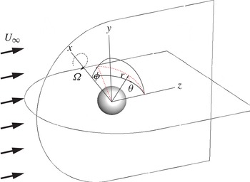
Figure 1 presents the problem geometry and the coordinate systems used in this study. A Cartesian coordinate system is aligned with the centre of the sphere. The free stream flows along the
 $z$
direction and the sphere rotation axis is constrained to the transverse
 $(x\text{-})$
axis only. A spherical coordinate system
 $(r,{\it\theta},{\it\phi})$
is also introduced for calculating the surface velocity distribution, where
 ${\it\theta}$
is the angle between the
 $z$
-axis and the
 $x$
-axis and
 ${\it\phi}$
is the angle between the
 $x$
-axis and the
 $y$
-axis.
The problem geometry and coordinate system used in CDP. The sphere is constrained to rotate in the transverse direction.

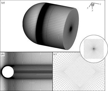
Figure 2(a) shows a typical computational domain. The dimensions of the computational domain are
 $$\begin{eqnarray}x^{\ast }=x/d\in \left[-15,15\right]\!,\quad y^{\ast }=y/d\in \left[-15,15\right]\!,\quad z^{\ast }=z/d\in \left[-15,20\right]\!.\end{eqnarray}$$
The computational domain comprises 6.94 million hexahedra cells. There are 280 cells along both the
 $x$
and
 $y$
directions, and approximately 500 cells are located downstream of the sphere. The grid is clustered towards the sphere surface ensuring that there are at least 10–15 cells within the boundary layer before flow separation and that there is sufficient resolution in the near wake (see figure 2
b). In figure 2(c), the arrangement of hexahedra cells near the centreline is presented in the
 $(x,y)$
-plane. A diamond shape arrangement of the hexahedra cells near the centreline (see inset in figure 2
c) avoids a numerical singularity when the mesh is rotated azimuthally to create the three-dimensional computational domain.
The unstructured-grid computational domain. (a) Isometric view, (b)
 $(x,z)$
-plane view and (c)
 $(x,y)$
-plane view downstream of the sphere showing the diamond centre section.

At the inlet
 $(z<0)$
and the outer cylindrical surface, a Dirichlet boundary condition
 $\boldsymbol{u}=(0,0,U_{\infty })$
is prescribed. The boundary condition is convective at the outlet. No-slip and no-penetration boundary conditions are employed on the sphere surface. The surface velocity distribution for a rotating sphere in Cartesian coordinates is
 $$\begin{eqnarray}\displaystyle \boldsymbol{u}|_{\partial {\it\Gamma}} & = & \displaystyle {\it\bf\Omega}\times \boldsymbol{r}\nonumber\\ \displaystyle & = & \displaystyle \frac{{\it\Omega}d}{2}[\left(-\text{cos}\,{\it\theta}\right)\boldsymbol{e}_{y}-\left(\sin {\it\phi}\sin {\it\theta}\right)\boldsymbol{e}_{z}].\end{eqnarray}$$
Initially, a uniform velocity field,
 $U_{\infty }$
, was defined throughout the computational domain. The simulations were carried out until the flow fields reached a statistically steady state. The corresponding flow fields were used as the initial condition for the flow past a rotating sphere at
 $\mathit{Re}=500{-}1000$
.
3. Code validation
The finite volume solver, CDP, has been extensively validated with experimental data for flow past a cylinder (Mahesh et al.
Reference Mahesh, Constantinescu and Moin2004) and flow past an aerofoil (Lopez & Moser Reference Lopez and Moser2008; You et al.
Reference You, Ham and Moin2008). In this section, results for the flow past a stationary sphere at
 $\mathit{Re}=500$
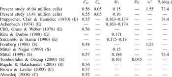
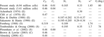
and 1000 are presented. The aim is to demonstrate the solver’s ability to capture the important flow physics behind a sphere. Tables 1 and 2 show that the important flow parameters calculated from the present study are in excellent agreement with the experimental data, numerical data and revisited correlations for sphere drag available in the open literature. The sensitivity of the spatial resolution is also presented in the tables. A decrease in the number of cells to 3.41 million results in negligible changes in the important flow parameters (see tables 1 and 2). In particular,
 $C_{D}$
remains accurate up to two significant digits. However, the numerical studies were performed using 6.94 million cells in order to provide a better resolution to the near-wake flow field and to ensure adequate spatial resolution once sphere rotation was enforced.
The sensitivity of the spatial resolution and comparison of the important flow parameters for
 $\mathit{Re}=500$
. The time-averaged drag coefficient,
 $C_{D}$
, lift coefficient,
 $C_{L}$
, Strouhal number,
 $St$
, non-dimensional wake length,
 $w^{\ast }$
(distance between the sphere centre and the tail of the recirculation bubbles), and separation angle,
 ${\it\theta}_{s}$
, are listed. E stands for experimental data, S for numerical data and C for correlations.

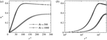
The boundary layer velocity profile for the flow past a stationary sphere at
 $\mathit{Re}=500$
and 1000. (a) Linear–linear scale and (b) linear–log scale to emphasise the adequate spatial resolution in the viscous sublayer.

The sensitivity of the spatial resolution and comparison of the important flow parameters for
 $\mathit{Re}=1000$
. The time-averaged drag coefficient,
 $C_{D}$
, lift coefficient,
 $C_{L}$
, Strouhal number,
 $St$
, non-dimensional wake length,
 $w^{\ast }$
(distance between the sphere centre and the tail of the recirculation bubbles), and separation angle,
 ${\it\theta}_{s}$
, are listed. E stands for experimental data, S for numerical data and C for correlations.

Evidence of adequate spatial resolution for all
 $\mathit{Re}$
and
 ${\it\Omega}^{\ast }$
considered will be discussed in detail. In DNS, it is important that the boundary layer before flow separation is well resolved. The number of cells within the boundary layer before flow separation for a stationary sphere at
 $\mathit{Re}=500$
and 1000 is presented in figure 3. The velocity is normalised by the friction velocity,
 $u_{{\it\tau}}=\sqrt{{\it\tau}_{w}/{\it\rho}}$
, where
 ${\it\tau}_{w}$
is the local wall shear stress. The normalised radial distance is
 $r^{+}=ru_{{\it\tau}}/{\it\mu}$
, where
 ${\it\mu}$
is the dynamic viscosity. At both Reynolds numbers, there are more than 15 cells within the boundary layer. Although the amount of cells shown is more than adequate, the same computational domain is employed for calculations of the flow past a transversely rotating sphere. Sphere rotation can reduce the boundary layer thickness as the local Reynolds number on the advancing side of the sphere (hemisphere where the sphere surface velocity vector opposes the free stream velocity) increases and thus requires a higher mesh resolution near the surface. The velocity profile is also plotted on a linear–log scale (see figure 3
b). The linear–log scale plot shows that there is sufficient resolution to capture the viscous sublayer region and a smooth velocity profile is predicted using the current computational domain.
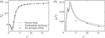
The time-averaged centreline velocity is presented in figure 4(a) and agrees well with experimental data from Wu & Faeth (Reference Wu and Faeth1993) and numerical data from Tomboulides & Orszag (Reference Tomboulides and Orszag2000). The non-dimensional wake length
 $(w^{\ast }\approx 1.85)$
, measured by locating
 $\overline{u^{\ast }}=0$
in figure 4(a), is in good agreement with the values listed in table 2. Figure 4(b) shows the RMS velocity profile along the centreline. Although the present study is in good agreement with the numerical data of Tomboulides & Orszag (Reference Tomboulides and Orszag2000), both differ from the experimental data of Wu & Faeth (Reference Wu and Faeth1993). Tomboulides & Orszag (Reference Tomboulides and Orszag2000) attributed this discrepancy to measurement errors in the experimental study.
Centreline velocity for
 $\mathit{Re}=1000$
. (a) Time-averaged centreline velocity and (b) RMS centreline velocity.

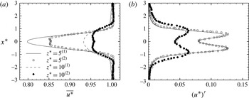
Figure 5 presents the time-averaged velocity deficit and RMS streamwise velocity at two locations downstream of the sphere. There are some differences in the velocity deficit near the centreline between the present study and Tomboulides & Orszag (Reference Tomboulides and Orszag2000). The discrepancy could be perhaps attributed to the increase in spatial resolution in the
 $x$
direction (
 ${\rm\Delta}x^{\ast }\approx 0.007$
in the presented study versus 0.013 as estimated from figure 2 in Tomboulides & Orszag Reference Tomboulides and Orszag2000). The RMS streamwise velocity shows excellent agreement.
The velocity deficit along the
 $x$
direction at 5 diameters and 10 diameters downstream for
 $\mathit{Re}=1000$
. (a) Time-averaged velocity deficit and (b) RMS streamwise velocity.
 $\text{}^{(1)}$
Present study and
 $\text{}^{(2)}$
Tomboulides & Orszag (Reference Tomboulides and Orszag2000).

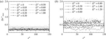
The implementation of the surface velocity distribution for a rotating sphere (2.4) is also verified against other published data (Giacobello et al. Reference Giacobello, Ooi and Balachandar2009; Kim Reference Kim2009; Poon et al. Reference Poon, Ooi, Giacobello and Cohen2010, Reference Poon, Ooi, Giacobello and Cohen2013). To ensure that the flow past a transversely rotating sphere is well resolved in the presented computational domain, the maximum size of all viscous wall units is presented in figure 6. The viscous wall unit in the radial direction is given as
 $$\begin{eqnarray}{\rm\Delta}r^{+}=\frac{{\rm\Delta}r\,u_{{\it\tau}}}{{\it\nu}},\end{eqnarray}$$
where
 ${\rm\Delta}r$
denotes the size of the first cell in the radial direction. For a bluff body flow,
 ${\rm\Delta}r^{+}\leqslant 1$
is required to ensure accurate prediction of the flow separation that leads to reverse flow in the near wake (Spalart & Squires Reference Spalart, Squires, McCallen, Browand and Ross2004). At
 $\mathit{Re}=500$
,
 ${\rm\Delta}{r^{+}}_{max}$
is always below 1 (the upper limit). However, for
 $\mathit{Re}=1000$
the instantaneous
 ${\rm\Delta}{r^{+}}_{max}$
at
 ${\it\Omega}^{\ast }=1.20$
occasionally exceeds 1. The significant increase in
 ${\rm\Delta}{r^{+}}_{max}$
is attributed to the increase in local relative velocity on the advancing side of the sphere. This increases the local Reynolds number,
 $\mathit{Re}_{l}=(U_{\infty }+{\it\Omega}d)d/2{\it\nu}=2200$
, and therefore requires more spatial resolution near the wall. Strictly speaking, this computational domain is not adequate for this set of simulation parameters. However, since the flow is separated and unsteady, it is reasonable to consider the upper bound (99.7 %) of the statistical Gaussian distribution of
 ${\rm\Delta}{r^{+}}_{max,u}$
, for which
 ${\rm\Delta}{r^{+}}_{max,u}=\overline{{\rm\Delta}{r^{+}}_{max}}+3{\rm\Delta}{r^{+}}_{max}^{\prime }=0.7907<1$
. As a result, the size of the first cell is deemed to be adequate for simulation at
 $\mathit{Re}=1000$
and
 ${\it\Omega}^{\ast }=1.20$
.
Maximum instantaneous viscous wall unit
 $({\rm\Delta}{r^{+}}_{max})$
of all wall-adjacent cells for (a)
 $\mathit{Re}=500$
and (b)
 $\mathit{Re}=1000$
.

The adequacy of the spatial resolution in the near wake is further verified by presenting the ratio of the grid spacing in the
 $z$
direction,
 ${\rm\Delta}z$
, to the Kolmogorov length scale,
 ${\it\eta}$
, for
 $\mathit{Re}=1000$
,
 ${\it\Omega}^{\ast }=0.00$
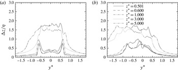
(stationary sphere) and 1.20 (highest rotational rate considered) in figure 7. Even though transverse rotation leads to substantial increase in
 ${\rm\Delta}z/{\it\eta}$
towards the advancing side of the sphere
 $(y^{\ast }<0)$
, the maximum
 ${\rm\Delta}z/{\it\eta}$
remains less than three for the highest
 $\mathit{Re}$
and
 ${\it\Omega}^{\ast }$
considered. According to Kurien & Taylor (Reference Kurien and Taylor2005), the spatial resolution is therefore sufficient. The temporal resolution is also checked against the Kolmogorov time scale and the time step used is at least two times smaller than the calculated Kolmogorov time scale.
The ratio of the grid spacing in the
 $z$
direction,
 ${\rm\Delta}z$
, to the Kolmogorov length scale,
 ${\it\eta}$
, at various locations downstream of the sphere for (a)
 $\mathit{Re}=1000$
,
 ${\it\Omega}^{\ast }=0.00$
and (b)
 $\mathit{Re}=1000$
,
 ${\it\Omega}^{\ast }=1.20$
.

4. Results and discussion
The flow past a transversely rotating sphere at
 $\mathit{Re}=500{-}1000$
is investigated for non-dimensional rotation rates
 ${\it\Omega}^{\ast }=0{-}1.20$
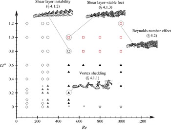
. The flow regimes are reported in figure 8 together with data available in the open literature (Giacobello et al.
Reference Giacobello, Ooi and Balachandar2009; Kim Reference Kim2009; Poon et al.
Reference Poon, Ooi, Giacobello and Cohen2010, Reference Poon, Ooi, Giacobello and Cohen2013). The flow past a transversely rotating sphere over the range of
 $\mathit{Re}$
and
 ${\it\Omega}^{\ast }$
considered can be classified into two previously reported regimes, the ‘vortex shedding’ and ‘shear layer instability’ regimes, and a new ‘shear layer–stable foci’ regime. The ‘vortex shedding’ regime is observed for
 $\mathit{Re}=500{-}1000$
at
 ${\it\Omega}^{\ast }\leqslant 0.60$
. Depending on
 ${\it\Omega}^{\ast }$
, the flow can either be planar-symmetric or asymmetric. The ‘shear layer instability’ regime is observed at
 $\mathit{Re}=500$
and
 ${\it\Omega}^{\ast }=0.80$
, whereas the ‘shear layer–stable foci’ regime occurs at
 $\mathit{Re}=500$
and
 ${\it\Omega}^{\ast }=1.00$
;
 $\mathit{Re}=640{-}1000$
and
 ${\it\Omega}^{\ast }\geqslant 0.80$
. It is important to note that the flow structures are sensitive to small variation in
 ${\it\Omega}^{\ast }$
, therefore no inference can be made about the flow structure expected between the discrete values simulated. In the following sections, the dynamic features of each flow regime and its effect on the near-wake flow fields are described in detail. A complete picture of the flow past a transversely rotating sphere at
 $\mathit{Re}=500$
and 1000 for all
 ${\it\Omega}^{\ast }$
considered is provided in the Appendix.
Different flow regimes for a transversely rotating sphere for low to moderate Reynolds numbers: ⬥, steady flow; +, oscillation vortex threads; ▴, vortex shedding; ○, shear layer instability; ▿, turbulent flow with laminar boundary layer; ▫, shear layer–stable foci. Symbols in grey represent data in the open literature. Symbols in red indicate the newly discovered regime. A representation of the isosurface of the instantaneous vortical structures for selected regime is also presented. Data for
 $\mathit{Re}\leqslant 300$
are obtained from Kim (Reference Kim2009), Giacobello et al. (Reference Giacobello, Ooi and Balachandar2009) and Poon et al. (Reference Poon, Ooi, Giacobello and Cohen2010, Reference Poon, Ooi, Giacobello and Cohen2013).

4.1. Flow past a transversely rotating sphere
4.1.1. Vortex shedding regime
The ‘vortex shedding’ regime has been reported by Giacobello et al. (Reference Giacobello, Ooi and Balachandar2009) and Kim (Reference Kim2009) for the flow past a transversely rotating sphere at
 $\mathit{Re}\leqslant 300$
and
 ${\it\Omega}^{\ast }\leqslant 0.30$
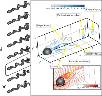
. Figure 9 presents the temporal evolution of the vortex shedding flow structures over a shedding period at
 $\mathit{Re}=500$
and
 ${\it\Omega}^{\ast }=0.20$
. Isosurfaces are identified using the
 ${\it\lambda}_{2}$
vortex identification method (Jeong & Hussain Reference Jeong and Hussain1995) by plotting an isosurface value
 ${\it\lambda}_{2}=-0.0008$
. In the ‘vortex shedding’ regime, the flow comprises horseshoe shape vortices (top of the flow structures) shed from the sphere and induced vortices (bottom of the flow structures) which connect the horseshoe shape vortices together. These flow structures are qualitatively similar to a stationary sphere at
 $\mathit{Re}=300$
(Johnson & Patel Reference Johnson and Patel1999) and a transversely rotating sphere at low
 $\mathit{Re}$
and
 ${\it\Omega}^{\ast }$
(Giacobello et al.
Reference Giacobello, Ooi and Balachandar2009; Kim Reference Kim2009) except that the flow loses
 $(y,z)$
-plane symmetry at certain
 ${\it\Omega}^{\ast }$
. For a clear illustration of the vortex shedding regime, planar-symmetric flow structures at
 $\mathit{Re}=500$
and
 ${\it\Omega}^{\ast }=0.20$
are presented.
The vortex shedding regime (
 $\mathit{Re}=500$
and
 ${\it\Omega}^{\ast }=0.20$
): temporal evolution of vortical structures (isosurfaces of
 ${\it\lambda}_{2}=-0.0008$
) over a shedding period. Snapshot of out-of-plane vorticities,
 ${\it\omega}_{i}$
, where the subscript
 $i=x$
,
 $y$
and
 $z$
, in the
 $(y,z)$
-plane, the
 $(x,z)$
-plane and a cross-stream plane at
 $z^{\ast }=5$
; the projected streamline patterns in the
 $(y,z)$
-plane are also shown. The projected streamlines are coloured by the out-of-plane velocity,
 $u_{x}$
.

To further analyse the effect of the sphere rotation on the near-wake flow field, instantaneous out-of-plane vorticities,
 ${\it\omega}_{i}$
, at five-eighths of the shedding period are presented in the
 $(x,z)$
-,
 $(y,z)$
- and cross-stream planes at
 $z^{\ast }=5.0$
(see figure 9). At this time instant, the shed vortex begins to separate from the sphere. The
 $x$
-vorticity,
 ${\it\omega}_{x}$
, in the
 $(y,z)$
-plane shows long finger-like negative contours on the advancing side of the sphere
 $(y^{\ast }<0)$
. A small patch of positive
 ${\it\omega}_{x}$
is also found in the near wake towards the advancing side of the sphere. This is because the sphere rotation expands the positive
 ${\it\omega}_{x}$
towards
 $y^{\ast }<0$
(Giacobello et al.
Reference Giacobello, Ooi and Balachandar2009). In the wake, a patch of vertical positive
 ${\it\omega}_{x}$
discharged previously is shown. In the
 $(x,z)$
-plane, the
 $y$
-vorticity changes rapidly from positive near the centreline to negative as
 $x^{\ast }$
increases. The tail of the negative
 ${\it\omega}_{y}$
rolls up where the shed vortex is located (see the isosurfaces of
 ${\it\lambda}_{2}$
). A separate patch of
 ${\it\omega}_{y}$
is shown further downstream. The location of this patch coincides with the legs of the induced vortex. The location of this patch of
 ${\it\omega}_{y}$
also indicates that the induced vortex is likely to be formed from the positive
 $x$
-vorticity in the
 $(y,z)$
-plane. In the cross-stream plane at
 $z^{\ast }=5.0$
, the negative
 $z$
-vorticity
 $({\it\omega}_{z})$
shows a kidney shape as the plane cuts through the horseshoe vortex (Giacobello et al.
Reference Giacobello, Ooi and Balachandar2009).
One of the main features of the ‘vortex shedding’ flow regime is the ‘buildup and release’ of the recirculation bubbles in the near wake (Johnson & Patel Reference Johnson and Patel1999). However, both Johnson & Patel (Reference Johnson and Patel1999) and Giacobello et al. (Reference Giacobello, Ooi and Balachandar2009) mentioned that the presence of the recirculation bubbles can be masked by the vorticity generated by the cylindrical shear layer in the near wake. As a result, to confirm the existence of the recirculation bubbles, the streamline pattern, which is coloured by the out-of-plane velocity
 $(u_{z})$
, projected in the
 $(y,z)$
-plane is necessary. The recirculation bubbles are clearly evident in the streamline pattern. As a result of the transverse sphere rotation, the recirculation bubbles are also displaced towards the advancing side of the sphere. The planar-symmetric flow structures result in
 $u_{x}\approx 0$
.
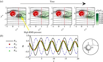
The effect of the ‘buildup and release’ of the recirculation bubbles in the ‘vortex shedding’ regime on the near-wake flow fields is shown by displaying the near-wake streamline pattern and RMS pressure in the
 $(y,z)$
-plane in figure 10(a), and the normalised cross-correlations at
 $(z^{\ast },r^{\ast })=(1.0,0.6)$
in the azimuthal direction in figure 10(b). The cross-correlation function is given as
 $$\begin{eqnarray}C_{IJ}=\lim _{T\rightarrow \infty }\frac{1}{T}\int _{0}^{T}u_{z},\text{}_{I}(t)u_{z},\text{}_{J}(t+{\it\tau})\text{d}t,\end{eqnarray}$$
where the subscripts
 $I$
and
 $J$
denote the signal locations of the streamwise velocity with
 $I,\,J=1$
, 2, 3 and 4, as shown in the inset of figure 10(b). In the present study, the normalised cross-correlation coefficients
 $R_{IJ}$
are presented, where
 $$\begin{eqnarray}R_{IJ}\left({\it\tau}\right)=\frac{C_{IJ}\left({\it\tau}\right)}{\sqrt{C_{II}\left(0\right)\,C_{JJ}\left(0\right)}},\end{eqnarray}$$
such that
 $R_{11}$
stands for the auto-correlation, and
 $R_{12}$
is the cross-correlation of
 $u_{z}$
between locations 1 and 2, etc.
(a) The effect of ‘vortex shedding’ on the near-wake streamline pattern and RMS pressure; (b) normalised cross-correlations,
 $R$
, versus time delay,
 ${\it\tau}$
, (see (4.2)) at
 $z^{\ast }=1.0$
(indicated by the red dashed line in a) for four azimuthal locations (see inset).

Due to the ‘buildup and release’ of the recirculation bubbles, the near wake
 $(z^{\ast }\approx 0.5{-}2.0)$
is highly unstable. This unstable near wake is clearly shown in the RMS pressure contour plots in the
 $(y,z)$
-plane where the patch of high RMS pressure coincides with the location of the recirculation bubbles at
 $z^{\ast }\approx 0.5{-}2.0$
. It should be noted that the RMS pressure is stronger on the advancing side of the sphere
 $(y^{\ast }<0)$
as the recirculation bubbles are displaced towards the advancing side of the sphere by the transverse sphere rotation. The cross-correlations of
 $u_{z}$
show that
 $R_{13}$
is anti-correlated (as
 $R_{13}({\it\tau}=0)\approx -1$
) and is
 ${\rm\pi}$
out-of-phase with
 $R_{11}$
. This anti-correlated and
 ${\rm\pi}$
out-of-phase behaviour is attributed to the alternating shed and induced vortices aligned with the
 $y$
-axis as a result of the ‘buildup and release’ mechanism. On the other hand,
 $R_{12}$
and
 $R_{14}$
are less correlated because the recirculation bubbles are ‘buildup and released’ in the
 $y$
direction.
4.1.2. Shear layer instability regime
The recirculation region on the retreating side of the sphere
 $(y^{\ast }>0)$
is progressively suppressed as
 ${\it\Omega}^{\ast }$
increases and the flow structures transform into the ‘shear layer instability’ regime at
 $\mathit{Re}=500$
and
 ${\it\Omega}^{\ast }=0.80$
, similarly to those at lower
 $\mathit{Re}$
(Giacobello et al.
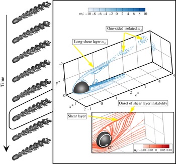
Reference Giacobello, Ooi and Balachandar2009; Kim Reference Kim2009). Temporal evolution of the ‘shear layer instability’ vortical structures is shown in figure 11. Differently from the ‘vortex shedding’ regime, the flow structures show double vortical threads in the near wake. These threads tilt and connect to form a one-sided hairpin structure further downstream. Giacobello et al. (Reference Giacobello, Ooi and Balachandar2009) reasoned that the formation of the one-sided vortices was due to the oblique Kelvin–Helmholtz instability.
Shear layer instability (
 $\mathit{Re}=500$
and
 ${\it\Omega}^{\ast }=0.80$
): temporal evolution of vortical structures (isosurfaces of
 ${\it\lambda}_{2}=-0.0008$
) over a shedding period. Snapshot of out-of-plane vorticities,
 ${\it\omega}_{i}$
, where the subscript
 $i=x$
,
 $y$
and
 $z$
, in the
 $(y,z)$
-plane,
 $(x,z)$
-plane and a cross-stream plane at
 $z^{\ast }=5$
; projected streamline patterns in the
 $(y,z)$
-plane are also shown. The projected streamlines are coloured by the out-of-plane velocity,
 $u_{x}$
.

A snapshot of the out-of-plane vorticities,
 ${\it\omega}_{i}$
, is also presented in figure 11. As
 ${\it\Omega}^{\ast }$
increases from 0.20 to 0.80, the positive
 $x$
-vorticity,
 ${\it\omega}_{x}$
, in the
 $(y,z)$
-plane is directed towards the advancing side of the sphere and is progressively shorter so that it almost becomes invisible. In the meantime, the increase in rotation rate increases flow shear on the advancing side of the sphere and results in a thinner but stronger negative
 ${\it\omega}_{x}$
. This negative
 ${\it\omega}_{x}$
clearly indicates the presence of the shear layer instabilities further downstream and forms isolated patches of negative vortices that represent the one-sided vortices in the flow structures. The shear layer instability is also quantified by Poon et al. (Reference Poon, Ooi, Giacobello and Cohen2013), who compared the Strouhal number of the unsteady shear layer to the analytical Strouhal number from the linear stability analysis. The
 $y$
-vorticity in the
 $(x,z)$
-plane shows elongated patches of positive
 ${\it\omega}_{y}$
near the centreline, but is negative in value near the surface of the sphere. In addition, the contour lines show no sign of waviness. This is because the Kelvin–Helmholtz instability is only observed on the advancing side of the sphere. The cross-stream plane at
 $z^{\ast }=5.0$
shows a relatively small patch of negative
 ${\it\omega}_{z}$
. However, the
 ${\it\omega}_{z}$
contours are more concentrated as the Kelvin–Helmholtz instability redistributes the shear layer vorticity (Giacobello et al.
Reference Giacobello, Ooi and Balachandar2009).
The instantaneous projected streamline pattern is presented at the bottom of the figure. Within the ‘shear layer instability’ regime, the recirculation bubbles are completely suppressed. The fluid on the retreating side of the sphere is vectored towards the advancing side and creates a shearing motion on the advancing side. The shear layer eventually becomes unstable and releases small vortices, as shown in the
 $x$
-vorticity in the
 $(y,z)$
-plane.
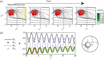
The shear layer is clearly evident in figure 12(a), which shows the temporal evolution of the streamline pattern. The shear layer is relatively stable in the near wake and instability only begins at
 $z^{\ast }\geqslant 2.0$
. As a result, the high RMS pressure is pushed downstream and is only evident near the onset of the shear layer instability (waviness of the streamlines at
 $z^{\ast }\geqslant 2.0$
). The transformation of flow from the ‘vortex shedding’ regime to the ‘shear layer instability’ regime also leads to a substantial change in the cross-correlations of
 $u_{z}$
, as shown in figure 12(b). Within the ‘shear layer instability’ regime,
 $R_{12}$
and
 $R_{14}$
become more anti-correlated than
 $R_{13}$
. In addition,
 $R_{13}$
is less anti-correlated for the ‘shear layer instability’ regime compared with the ‘vortex shedding’ regime
 $(R_{13\text{-}vortex\;shedding}>R_{13\text{-}shear\;layer\;instab.}\text{ at }{\it\tau}=0)$
. The physical reason for this change in cross-correlations can be attributed to the one-sided vortices that scale with the shear layer on the advancing side of the sphere (Giacobello et al.
Reference Giacobello, Ooi and Balachandar2009). As a result, the flow on the retreating side of the sphere is less affected by the instability of the shear layer. Similarly, the increasing anti-correlated
 $R_{12}$
and
 $R_{14}$
can be attributed to the locations of 2 and 4 being closer to the shear layer.
(a) The effect of ‘shear layer instability’ on the near-wake streamline pattern and RMS pressure; (b) normalised cross-correlations,
 $R$
, versus time delay,
 ${\it\tau}$
, (see (4.2)) at
 $z^{\ast }=1.0$
(indicated by the red dashed line in a) for four azimuthal locations (see inset).

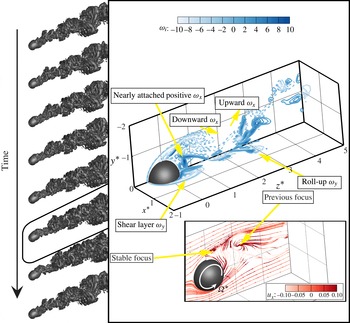
4.1.3. Shear layer–stable foci regime
A newly discovered flow regime is observed above the ‘shear layer instability’ regime at
 $\mathit{Re}=500$
and
 ${\it\Omega}^{\ast }=1.00$
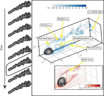
. This flow regime is denoted the ‘shear layer–stable foci’ regime. Figure 13 shows the temporal evolution of the flow structures with the instantaneous out-of-plane vortices and projected streamlines for this newly discovered regime. The flow structures become chaotic in the ‘shear layer–stable foci’ regime. Vortex loops roll up in different directions and form a ‘zigzag’ pattern in the wake. Although the vortex loops are no longer rolling up in a unidirectional manner, the orientation of these vortex loops is far from random. Vortex loops are either rolling up towards the advancing side of the sphere or at a slight angle. This vortex loop roll-up at an angle contributes to the sideways oriented vortex loops further downstream.
‘Shear layer–stable foci’ regime (
 $\mathit{Re}=500$
and
 ${\it\Omega}^{\ast }=1.00$
): temporal evolution of vortical structures (isosurfaces of
 ${\it\lambda}_{2}=-0.0008$
) over a shedding period. Snapshot of out-of-plane vorticities,
 ${\it\omega}_{i}$
, where the subscript
 $i=x$
,
 $y$
and
 $z$
, in the
 $(y,z)$
-plane,
 $(x,z)$
-plane and a cross-stream plane at
 $z^{\ast }=5$
; projected streamline patterns in the
 $(y,z)$
-plane are also shown. The projected streamlines are coloured by the out-of-plane velocity,
 $u_{x}$
.

The chaotic pattern of the flow structures can be explained in detail using the out-of-plane vorticities
 ${\it\omega}_{i}$
. A further increase of
 ${\it\Omega}^{\ast }$
from 0.80 to 1.00 shows an intensified (highly negative) shear layer vorticity
 ${\it\omega}_{x}$
on the advancing side of the sphere in the
 $(y,z)$
-plane. The shear layer vorticity is significantly shortened at this rotation rate and vortices of negative
 ${\it\omega}_{x}$
are released from the shear layer as early as
 $z^{\ast }\approx 1.0$
. Furthermore, a patch of positive
 ${\it\omega}_{x}$
is formed near the centreline at
 $z^{\ast }\approx 1.0$
below the first vortex that is released from the shear layer instability. This positive
 ${\it\omega}_{x}$
is detached from the lee side of the sphere and interacts with the negative
 ${\it\omega}_{x}$
to form a chaotic flow pattern in the wake comprising small patches of both positive and negative
 ${\it\omega}_{x}$
vortices. The flow unsteadiness near the centreline is also demonstrated by the waviness of positive
 ${\it\omega}_{y}$
in the
 $(x,z)$
-plane. As most of the vortices are released from the shear layer on the advancing side of the sphere, this unsteady
 ${\it\omega}_{y}$
motion near the centreline at
 $z^{\ast }\approx 2.0$
may be localised. In the cross-stream plane at
 $z^{\ast }=5.0$
, the interaction of the positive
 ${\it\omega}_{x}$
with the negative
 ${\it\omega}_{x}$
from the shear layer has led to small patches of positive and negative
 ${\it\omega}_{z}$
.
The instantaneous projected streamline pattern is shown at the bottom of the figure. The streamline pattern has a topology similar to those at
 ${\it\Omega}^{\ast }=0.80$
except that a stable focus (Chong, Perry & Cantwell Reference Chong, Perry and Cantwell1990) is formed on the advancing side of the sphere at
 $z^{\ast }\approx 1.0$
. The formation of this stable focus is different from the recirculation bubbles shown in the ‘vortex shedding’ regime (refer to figure 9). One of the major differences is that this stable focus is located near the onset of the shear layer instability rather than on the lee side of the sphere. The presence of the stable focus near the onset of the shear layer instability leads to an increase in flow unsteadiness in the near wake. The increase in flow unsteadiness below the stable focus at
 $z^{\ast }\approx 1.0$
explains the reappearance of the positive
 ${\it\omega}_{x}$
in the
 $(y,z)$
-plane. As a result of this stable focus near the onset of shear layer instability, small patches of positive and negative
 ${\it\omega}_{x}$
vortices in the
 $(y,z)$
-plane are thus shown in the wake. The presence of the stable focus also contributes to the ‘zigzag’ pattern of the vortex loops in the wake as there is a significant increase in velocity
 $(u_{x})$
both into and out of the
 $(y,z)$
-plane.
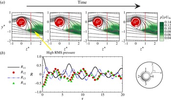
Figure 14(a) shows the temporal evolution of the stable focus over a shedding period. The stable focus oscillates in size as it convects downstream and results in highly unsteady flow on the advancing side of the sphere at
 $z^{\ast }>0.5$
. The increase in flow unsteadiness in this region leads to a substantial increase in pressure fluctuations on the advancing side of the sphere at
 $z^{\ast }>0.5$
, as shown in the RMS pressure contours. The cross-correlations
 $R_{12}$
,
 $R_{13}$
and
 $R_{14}$
in figure 14(b) show that the flow no longer comprises a single frequency in this flow regime. The second frequency may be linked to the existence of the stable focus. Apart from showing higher frequency oscillations, the cross-correlations for the ‘shear layer–stable foci’ regime show similar behaviour to the ‘shear layer instability’ regime, i.e.
 $R_{12}$
and
 $R_{14}$
are more anti-correlated than
 $R_{13}$
as a result of the shear layer instability on the advancing side of the sphere. In conclusion, it is observed that
 $R_{12}$
and
 $R_{14}$
become more anti-correlated than
 $R_{13}$
as the flow transforms from the ‘vortex shedding’ regime to either the ‘shear layer instability’ or the ‘shear layer–stable foci’ regime.
(a) The effect of ‘shear layer–stable foci’ on the near-wake streamline pattern and RMS pressure; (b) normalised cross-correlations,
 $R$
, versus time delay,
 ${\it\tau}$
, (see (4.2)) at
 $z^{\ast }=1.0$
(indicated by the red dashed line in a) for four azimuthal locations (see inset).

4.2. Effect of Reynolds number on the shear layer–stable foci regime
Figure 15 presents the flow past a transversely rotating sphere at
 $\mathit{Re}=1000$
and
 ${\it\Omega}^{\ast }=1.20$
. As the vortices are scaled with the shear layer in the ‘shear layer–stable foci’ regime, increasing
 $\mathit{Re}$
and
 ${\it\Omega}^{\ast }$
result in smaller vortices in the wake. On the other hand, the flow structures display some kind of large-scale shedding pattern qualitatively similar to that in the ‘vortex shedding’ regime. Although the large-scale shedding pattern of the ‘roll-up and release’ of the small vortices from the Kelvin–Helmholtz instability was also reported for a stationary sphere at
 $\mathit{Re}=3700$
(Yun, Kim & Choi Reference Yun, Kim and Choi2006), the large-scale shedding pattern observed here is attributed to the presence of the stable focus near the onset of shear layer instability and will be discussed in detail.
Effect of Reynolds number on the ‘shear layer–stable foci’ (
 $\mathit{Re}=1000$
and
 ${\it\Omega}^{\ast }=1.20$
) vortical structures (isosurfaces of
 ${\it\lambda}_{2}=-0.0008$
) over a shedding period. Snapshot of out-of-plane vorticities,
 ${\it\omega}_{i}$
, where the subscript
 $i=x$
,
 $y$
and
 $z$
, in the
 $(y,z)$
-plane,
 $(x,z)$
-plane and a cross-stream plane at
 $z^{\ast }=5$
; projected streamline patterns in the
 $(y,z)$
-plane are also shown. The projected streamlines are coloured by the out-of-plane velocity,
 $u_{x}$
.

Before we present the instantaneous streamline pattern and discuss the effect of
 $\mathit{Re}$
on the stable focus, the out-of-plane vorticities
 $({\it\omega}_{i})$
are described. In the
 $(y,z)$
-plane, the negative
 $x$
-vorticity shear layer is substantially shortened. The patch of positive
 ${\it\omega}_{x}$
is also brought upstream and is nearly attached to the downstream pole of the sphere. This
 $x$
-vorticity patch is drawn upward in the negative
 $y$
direction and interacts with the negative vorticity near the onset of the shear layer instability. The interaction between the positive and negative vorticity patches draws the
 $x$
-vorticity downward. Further downstream, other patches of vorticity are shown vectoring upward again forming a vortex-shedding-like pattern in the
 $(y,z)$
-plane. In the
 $(x,z)$
-plane, the small patch of
 $y$
-vorticity
 $({\it\omega}_{y})$
in the near wake clearly indicates the shortened shear layer at this
 $\mathit{Re}$
and
 ${\it\Omega}^{\ast }$
. A patch of positive
 ${\it\omega}_{y}$
begins to roll up in the horizontal direction in the wake
 $(z^{\ast }\approx 2.0{-}3.0)$
. In the cross-stream plane at
 $z^{\ast }=5.0$
, only a small patch of the negative
 ${\it\omega}_{y}$
is observed.
The instantaneous projected streamline pattern is also shown in the figure. The streamlines on the retreating side of the sphere
 $(y^{\ast }>0)$
are clearly vectored towards the advancing side of the sphere, suppressing any shear layer instability of the Kelvin–Helmholtz type on the retreating side, as observed for flow past a stationary sphere at
 $\mathit{Re}=1000$
(Kim & Durbin Reference Kim and Durbin1988; Sakamoto & Haniu Reference Sakamoto and Haniu1990; Bonneton & Chomax Reference Bonneton and Chomax1992; Tomboulides & Orszag Reference Tomboulides and Orszag2000). These streamlines join those of the advancing side and result in shear layer instability of the Kelvin–Helmholtz type. Due to the high local Reynolds number
 $(\mathit{Re}_{l}=2200)$
, the onset of shear layer instability is pushed further upstream and the stable focus (Chong et al.
Reference Chong, Perry and Cantwell1990) is formed immediately behind the sphere. In addition, it is shown in the figure that the previous stable focus diffuses quickly as it convects downstream, drawing the streamlines towards the bottom of the plane. This explains the downward motion of the
 $x$
-vorticity at
 $z^{\ast }\approx 1.0{-}2.0$
. However, the surrounding flow is continuously drawn upward by the sphere rotation; the flow structures therefore exhibit a large-scale shedding pattern.
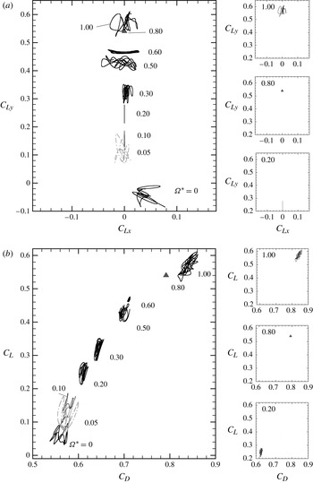
(a) Phase diagram
 $(C_{Ly},C_{Lx})$
and (b) phase diagram
 $(C_{L},C_{D})$
for a transversely rotating sphere at
 $\mathit{Re}=500$
.

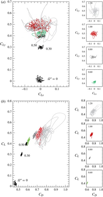
(a) Phase diagram
 $(C_{Ly},C_{Lx})$
and (b) phase diagram
 $(C_{L},C_{D})$
for a transversely rotating sphere at
 $\mathit{Re}=1000$
.

4.3. Hydrodynamic force coefficients for a transversely rotating sphere at
 $\mathit{Re}=500{-}1000$

The dynamic behaviour of the lift and drag coefficients acting on a transversely rotating sphere at
 $\mathit{Re}=500$
and 1000 is reported using phase diagrams of
 $(C_{Ly},C_{Lx})$
and
 $(C_{L},C_{D})$
in figures 16 and 17. All flow solutions are unsteady at these Reynolds numbers, but some solutions may appear to be steady due to the scaling of the phase diagram. These solutions are represented by a solid delta (▴). At
 $\mathit{Re}=500$
and
 ${\it\Omega}^{\ast }=0$
,
 $C_{Lx}$
and
 $C_{Ly}$
change irregularly and show a preferential orientation towards the positive
 $C_{Lx}$
-axis within a finite period of time; this was also reported by Mittal, Wilson & Najjar (Reference Mittal, Wilson and Najjar2002). As the sphere rotates, the preferential direction of lift changes from the positive
 $C_{Lx}$
-axis to the positive
 $C_{Ly}$
-axis due to the pressure differential created by a transversely rotating sphere. Increasing
 ${\it\Omega}^{\ast }$
decreases the oscillation magnitudes of
 $C_{Ly}$
for
 ${\it\Omega}^{\ast }\leqslant 0.60$
. As
 ${\it\Omega}^{\ast }$
increases from 0.50 to 0.60, the recirculation bubble on the retreating side of the sphere is almost suppressed. Therefore, although the flow structures are qualitatively similar as they are both within the ‘vortex shedding’ regime, the smaller recirculation bubble induces lower pressure fluctuation in the near wake and leads to a decrease in
 $C_{Ly}$
oscillation magnitudes. This decrease in lift coefficient fluctuation is most obvious as the flow enters the ‘shear layer instability’ regime where the recirculation bubbles are completely suppressed (see figure 12). Further increase in
 ${\it\Omega}^{\ast }$
to 1.00 leads to the formation of stable foci. These stable foci oscillate vigorously as they travel downstream (as shown in figure 14) and increase the pressure fluctuation in the near wake. As a result, both
 $C_{Lx}$
and
 $C_{Ly}$
oscillation magnitudes increase substantially.
Similar behaviour is observed for
 $C_{L}$
and
 $C_{D}$
at
 $\mathit{Re}=500$
. At
 ${\it\Omega}^{\ast }\leqslant 0.60$
(within the ‘vortex shedding’ regime), both
 $C_{L}$
and
 $C_{D}$
show large oscillations. Here,
 $C_{L}$
and
 $C_{D}$
decrease their oscillation magnitudes as the flow enters the ‘shear layer instability’ regime at
 ${\it\Omega}^{\ast }=0.80$
, but increase their oscillation magnitudes dramatically at
 ${\it\Omega}^{\ast }=1.00$
due to the oscillations of the stable foci.
At
 $\mathit{Re}=1000$
and
 ${\it\Omega}^{\ast }=0.00$
, the lift coefficients
 $C_{Ly}$
and
 $C_{Lx}$
again change irregularly with time but do not show a preferential direction. For a transversely rotating sphere at
 ${\it\Omega}^{\ast }\leqslant 0.60$
, even though the flow is within the ‘vortex shedding’ regime, the oscillation amplitudes of
 $C_{Ly}$
and
 $C_{Lx}$
are relatively small. Above
 ${\it\Omega}^{\ast }=0.80$
, the flow transforms to the ‘shear layer–stable foci’ regime and there is a slight increase in both
 $C_{Lx}$
and
 $C_{Ly}$
oscillation amplitudes. Their oscillation amplitudes increase dramatically for
 ${\it\Omega}^{\ast }\geqslant 1.00$
. The reason for the smaller oscillation amplitudes of
 $C_{Ly}$
at
 ${\it\Omega}^{\ast }\leqslant 0.60$
is attributed to the presence of the shear layer instability on the advancing side of the sphere. Giacobello et al. (Reference Giacobello, Ooi and Balachandar2009), Kim (Reference Kim2009) and Poon et al. (Reference Poon, Ooi, Giacobello and Cohen2013) showed that eddies released from the Kelvin–Helmholtz instability of the shear layer reduce the unsteadiness of the near-wake flow field. On the other hand, the oscillations of the stable foci contribute to the increase in
 $C_{Lx}$
and
 $C_{Ly}$
oscillation amplitudes. As
 ${\it\Omega}^{\ast }$
increases, these stable foci oscillate more vigorously and thus large oscillation amplitudes of
 $C_{Lx}$
and
 $C_{Ly}$
are observed.
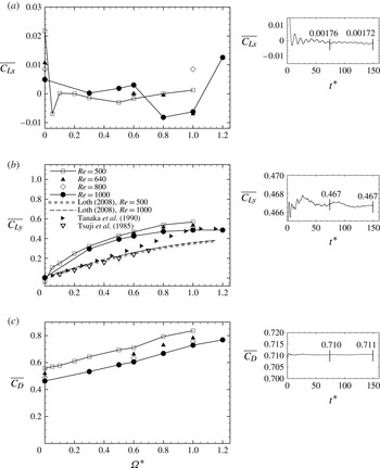
Time-averaged force coefficients for the flow past a stationary and transversely rotating sphere at
 $\mathit{Re}=500{-}1000$
: (a)
 $\overline{C_{Lx}}$
against
 ${\it\Omega}^{\ast }$
; (b)
 $\overline{C_{Ly}}$
against
 ${\it\Omega}^{\ast }$
; (c)
 $\overline{C_{D}}$
against
 ${\it\Omega}^{\ast }$
. The effect of integration time on the time-averaged force coefficients is shown in the insets for a sample parameter
 $(\mathit{Re}=500\text{ and }{\it\Omega}^{\ast }=0.60)$
. Time-averaged force coefficients are displayed at half integration time and full integration time.

Both
 $C_{L}$
and
 $C_{D}$
at
 $\mathit{Re}=1000$
show low oscillation amplitudes within the ‘vortex shedding’ regime
 $({\it\Omega}^{\ast }\leqslant 0.60)$
. This is again related to the formation of the shear layer instability of the Kelvin–Helmholtz type on the advancing side of the sphere. On the other hand, for
 ${\it\Omega}^{\ast }\geqslant 0.80$
the stable foci oscillate and result in a substantial increase in the oscillation amplitudes of both
 $C_{L}$
and
 $C_{D}$
.
4.4. Time-averaged force coefficients for a transversely rotating sphere at
$\mathit{Re}=500{-}1000$

The time-averaged force coefficients acting on a stationary and transversely rotating sphere at
 $\mathit{Re}=500$
and 1000 are presented in figure 18. In all cases, the force coefficients are averaged over
 $t^{\ast }=150$
, which is equivalent to approximately 25 shedding periods for the flow past a stationary sphere at
 $\mathit{Re}=500{-}1000$
. The effect of time integration is demonstrated in the insets of figure 18 for a sample parameter at
 $\mathit{Re}=500$
and
 ${\it\Omega}^{\ast }=0.60$
. Convergence criteria are set such that the variation in time-averaged force coefficients is within 3 % of the value obtained at half the integration time interval. The time-averaged lift coefficient in the
 $x$
direction,
 $\overline{C_{Lx}}$
, is presented in figure 18(a);
 $\overline{C_{Lx}}\approx 0$
for all
 $\mathit{Re}$
and
 ${\it\Omega}^{\ast }$
considered beside a stationary sphere at
 $\mathit{Re}=500$
and a transversely rotating sphere at
 $\mathit{Re}=1000$
and
 ${\it\Omega}^{\ast }=1.20$
. The non-zero
 $\overline{C_{Lx}}$
for a stationary sphere at
 $\mathit{Re}=500$
may be attributed to flow structures showing a preferential orientation. Similar findings were also reported by Bagchi, Ha & Balachandar (Reference Bagchi, Ha and Balachandar2001) and Mittal et al. (Reference Mittal, Wilson and Najjar2002). Such preferential orientation is also observed for
 $\mathit{Re}=1000$
and
 ${\it\Omega}^{\ast }=1.20$
as a result of the vigorous oscillations of the stable foci near the onset of shear layer instability and leads to a non-zero
 $\overline{C_{Lx}}$
. However, it is important to note that this preferential orientation of the flow may not exist over a longer integration time and thus results in
 $\overline{C_{Lx}}\rightarrow 0$
(Yun et al.
Reference Yun, Kim and Choi2006). Although
 $\overline{C_{Lx}}$
may approach zero as the preferential orientation ceases over a longer integration time, a transversely rotating sphere always induces flow in the
 $y$
directions due to the ‘Robins–Magnus’ effect (see figures 9, 11, 13 and 15). As a result, time integration over 25 shedding periods that results in 3 % variation in
 $\overline{C_{Ly}}$
is considered adequate. In general,
 $\overline{C_{Ly}}$
increases with
 ${\it\Omega}^{\ast }$
, but decreases with
 $\mathit{Re}$
. However, the sensitivity of
 $\overline{C_{Ly}}$
to
 ${\it\Omega}^{\ast }$
decreases as
 ${\it\Omega}^{\ast }$
increases. Poon et al. (Reference Poon, Ooi, Giacobello and Cohen2010) reasoned that the decrease in sensitivity is due to the physical limit on the flow separation. Experimental results from Tsuji et al. (Reference Tsuji, Morikawa and Mizuno1985) as well as the correlation models of Tanaka et al. (Reference Tanaka, Yamagata and Tsuji1990) and Loth (Reference Loth2008) are also included. It is observed that experimental results reported a smaller
 $\overline{C_{Ly}}$
for a given
 ${\it\Omega}^{\ast }$
. On the other hand, Tanaka et al.’s correlation model was derived for subcritical
 $\mathit{Re}$
, but was shown to show good agreement with
 $\overline{C_{Ly}}$
at low
 $\mathit{Re}$
by Loth (Reference Loth2008). It is also important to mention that Loth’s model, although it gives a smaller
 $\overline{C_{Ly}}$
compared with our numerical results, provides a good agreement with the experimental results as it is mainly derived from the experimental data. The time-averaged resultant drag coefficient,
 $\overline{C_{D}}$
, is presented in figure 18(c). In brief,
 $\overline{C_{D}}$
increases with
 ${\it\Omega}^{\ast }$
but decreases with
 $\mathit{Re}$
.
The smaller experimental
 $\overline{C_{Ly}}$
may be attributed to the difficulties in maintaining a constant sphere rotation rate as the rotating sphere travels through a stationary viscous medium (Tsuji et al.
Reference Tsuji, Morikawa and Mizuno1985; Tri et al.
Reference Tri, Oesterle and Deneu1990). Tsuji et al. (Reference Tsuji, Morikawa and Mizuno1985) estimated that the sphere rotation decreases at a rate proportional to the viscous torque,
 $T$
, on the moment of inertia,
 $I$
, of the sphere, i.e.
 $\text{d}{\it\Omega}/\text{d}t=-T/I$
. However, the viscous torque acting on the sphere was only estimated based on the numerical results of Dennis, Singh & Ingham (Reference Dennis, Singh and Ingham1980). Bagchi & Balachandar (Reference Bagchi and Balachandar2002) performed a similar study numerically on the motion of a sphere in a linear shear flow and concluded that the sphere shows a faster decay rate for its rotating motion than its translation motion at finite Reynolds numbers. The ratio of the rotation decay,
 ${\it\tau}_{r}$
, to the translation decay,
 ${\it\tau}_{t}$
, lies between 0 and 0.3. Although the above expression was derived for a sphere that is free to translate and rotate in a linear shear flow, one would also expect similar decay behaviour for a sphere translating and rotating in a stationary viscous medium. Other uncertainties in measuring the sphere rotation rate, the sphere trajectory and its axis of rotation may contribute to the difference between experimental and numerical lift coefficients. In fact, Oesterlé & Dinh (Reference Oesterlé and Dinh1998) stated an error of 20 % in determining the sphere rotation rate. Tsuji et al. (Reference Tsuji, Morikawa and Mizuno1985) also reported a wide range of sphere rotation rates from their experimental set-up and the reported rotation rates are averaged over 100 trials. Furthermore, Bagchi & Balachandar (Reference Bagchi and Balachandar2003) showed that the effect of free stream disturbance, which is often difficult to remove experimentally, displays a small effect on the lift coefficient for a non-rotating sphere. The effect of free stream disturbance may become more pronounced as the sphere rotates due to the wake structures being sensitive to the modest changes in
 $\mathit{Re}$
and
 ${\it\Omega}^{\ast }$
.
The time-averaged resultant force coefficients
 $(\overline{C_{D}}\text{ and }\overline{C_{Ly}})$
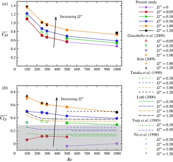
versus Reynolds numbers for the flow past a stationary and transversely rotating sphere are presented in figure 19. The numerical data for laminar Reynolds numbers obtained in Giacobello et al. (Reference Giacobello, Ooi and Balachandar2009), Kim (Reference Kim2009) and Poon et al. (Reference Poon, Ooi, Giacobello and Cohen2010), experimental data from Tsuji et al. (Reference Tsuji, Morikawa and Mizuno1985), Tanaka et al. (Reference Tanaka, Yamagata and Tsuji1990) and Tri et al. (Reference Tri, Oesterle and Deneu1990), and the lift correlation model by Loth (Reference Loth2008) are also superimposed onto the figure. In general, the resultant drag coefficient,
 $\overline{C_{D}}$
, increases with
 ${\it\Omega}^{\ast }$
but decreases with
 $\mathit{Re}$
. On the other hand, although the time-averaged lift coefficient,
 $\overline{C_{Ly}}$
, increases with the dimensionless rotation rate,
 ${\it\Omega}^{\ast }$
, it shows two different behaviours (highlighted in figure 19
a by white and grey colour) with increasing
 $\mathit{Re}$
. At low
 ${\it\Omega}^{\ast }\ ({\it\Omega}^{\ast }\leqslant 0.30)$
,
 $\overline{C_{Ly}}$
increases initially and decreases after reaching a maximum as
 $\mathit{Re}$
increases. However, for higher rotation rate
 $({\it\Omega}^{\ast }\geqslant 0.50)$
, all calculations show a monotonic decrease in
 $\overline{C_{Ly}}$
with
 $\mathit{Re}$
. It is also important to remember that the flow structures for a stationary sphere may show a preferential direction over the time integration of 25 shedding periods. As a result of this historical bias in data collected,
 $\overline{C_{Ly}}$
shows a significant magnitude at these considered Reynolds numbers.
Time-averaged resultant force coefficients against Reynolds number for the flow past a stationary and transversely rotating sphere: (a)
 $\overline{C_{D}}$
and (b)
 $\overline{C_{Ly}}$
. The grey box highlights the change in behaviour in
 $\overline{C_{Ly}}$
with
 $\mathit{Re}$
.

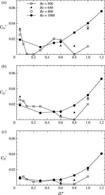
RMS force coefficients for the flow past a stationary and transversely rotating sphere at
 $\mathit{Re}=500{-}1000$
: (a)
 ${C_{Lx}}^{\prime }$
against
 ${\it\Omega}^{\ast }$
; (b)
 ${C_{Ly}}^{\prime }$
against
 ${\it\Omega}^{\ast }$
; (c)
 ${C_{D}}^{\prime }$
against
 ${\it\Omega}^{\ast }$
.

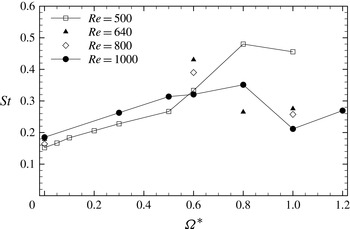
Strouhal number,
 $St$
, versus dimensionless rotation rate,
 ${\it\Omega}^{\ast }$
, for a transversely rotating sphere.

In early sections of this paper, it was mentioned that the stable foci oscillate vigorously and lead to a significant increase in the near-wake RMS pressure fluctuations and thus higher oscillation magnitudes for the force coefficients. Here, we quantify this effect by presenting the RMS force coefficients. In figure 20(a), the RMS force coefficient fluctuation,
 ${C_{Lx}}^{\prime }$
, in the
 $x$
direction is presented. Here,
 ${C_{Lx}}^{\prime }>0$
for all cases considered except for
 $\mathit{Re}=500$
and
 ${\it\Omega}^{\ast }=0.20$
. It should be noted that for
 $\mathit{Re}=500$
and
 ${\it\Omega}^{\ast }=0.80$
,
 ${C_{Lx}}^{\prime }$
is slightly above zero. In addition, it is observed that as the flow enters the newly discovered ‘shear layer–stable foci’ regime, there is a substantial increase in
 ${C_{Lx}}^{\prime }$
for both Reynolds numbers. Here,
 ${C_{Lx}}^{\prime }=0$
at
 $\mathit{Re}=500$
and
 ${\it\Omega}^{\ast }=0.20$
due to the fact that the flow remains planar-symmetric about the
 $(y,z)$
-plane. For
 ${C_{Ly}}^{\prime }$
at
 $\mathit{Re}=500$
, it is evident in figure 20(b) that with increasing
 ${\it\Omega}^{\ast }$
,
 ${C_{Ly}}^{\prime }$
decreases and reaches a minimum at
 ${\it\Omega}^{\ast }=0.80$
;
 ${C_{Ly}}^{\prime }$
increases dramatically at
 ${\it\Omega}^{\ast }=1.00$
. For
 $\mathit{Re}=1000$
,
 ${C_{Ly}}^{\prime }$
also decreases initially with
 ${\it\Omega}^{\ast }$
. However,
 ${C_{Ly}}^{\prime }$
increases substantially at
 ${\it\Omega}^{\ast }\geqslant 0.80$
when the flow enters the ‘shear layer–stable foci’ regime. The results for
 $\mathit{Re}=640$
and 800 show a similar increase in
 ${C_{Ly}}^{\prime }$
for
 ${\it\Omega}^{\ast }\geqslant 0.80$
. A similar behaviour is also observed for
 ${C_{D}}^{\prime }$
in figure 20(c). Hence, it can be concluded that the presence of stable foci leads to an increase in the RMS force coefficients for the Reynolds numbers considered.
The Strouhal number,
 $St$
, versus the dimensionless rotation rate,
 ${\it\Omega}^{\ast }$
, is presented in figure 21. The Strouhal number is calculated by averaging the frequency of the streamwise velocity,
 $u_{z}$
, at
 $(z^{\ast },r^{\ast })=(2.5,0.6)$
in the azimuthal direction. Only the dominant frequency, which is the frequency corresponding to the most energetic mode, is presented. For
 $\mathit{Re}=500$
, the Strouhal number monotonically increases for
 ${\it\Omega}^{\ast }\leqslant 0.80$
before decreasing slightly. There is also a substantial increase in
 $St$
for
 ${\it\Omega}^{\ast }=0.80$
compared with lower
 ${\it\Omega}^{\ast }$
. For
 $\mathit{Re}=1000$
,
 $St$
increases for
 ${\it\Omega}^{\ast }\leqslant 0.80$
. For
 ${\it\Omega}^{\ast }=1.00$
, there is a sudden decrease in
 $St$
, but it increases again for
 ${\it\Omega}^{\ast }=1.20$
. For
 $\mathit{Re}=640$
and 800, high
 $St$
is observed at
 ${\it\Omega}^{\ast }=0.60$
. Here,
 $St$
decreases significantly at
 $\mathit{Re}=640$
and
 ${\it\Omega}^{\ast }=0.80$
. At
 ${\it\Omega}^{\ast }=1.00$
, both values of
 $\mathit{Re}$
show similar values of
 $St$
and are closer to the one at
 $\mathit{Re}=1000$
.
5. Conclusions
Direct numerical simulation of the flow past a transversely rotating sphere was investigated beyond the laminar Reynolds number range at
 $\mathit{Re}=500{-}1000$
, and for dimensionless rotation rates between
 ${\it\Omega}^{\ast }=0$
and 1.20. The accuracy of the solver was validated against existing experimental and numerical data. The spatial and temporal resolutions were checked with both Kolmogorov length and time scales, and wall
 $(+)$
units.
By studying the unsteadiness of the flow structures at
 $\mathit{Re}=500{-}1000$
and other numerical results reported previously, three main flow regimes can be observed at
 $\mathit{Re}=500{-}1000$
. These are the ‘vortex shedding’, ‘shear layer instability’ and a newly discovered ‘shear layer–stable foci’ regimes. The new regime is found at
 $\mathit{Re}=500$
and
 ${\it\Omega}^{\ast }=1.00$
;
 $\mathit{Re}=640{-}1000$
and
 ${\it\Omega}^{\ast }\geqslant 0.80$
. In this regime, a stable focus is observed near the onset of shear layer instability. The existence of the stable focus near the onset of shear layer instability results in highly unsteady flow in that region and thus increases the RMS pressure. The stable focus becomes more pronounced at
 $\mathit{Re}=1000$
and
 ${\it\Omega}^{\ast }=1.20$
. The increase in
 $\mathit{Re}$
further shortens the shear layer on the advancing side of the sphere. Small-scale vortices released from the shear layer interact with the stable focus to form large-scale shedding patterns. In addition, the more pronounced stable focus dramatically increases the RMS pressure aft of the sphere and thus increases the RMS force coefficients significantly. Numerical studies of the flow past a transversely rotating sphere also reveal two distinctive behaviours of
 $\overline{C_{Ly}}$
across the
 $\mathit{Re}$
range considered. At low
 ${\it\Omega}^{\ast }\leqslant 0.30$
,
 $\overline{C_{Ly}}$
increases with
 $\mathit{Re}$
and reaches a maximum before decreasing. In contrast,
 $\overline{C_{Ly}}$
shows a monotonic decrease with
 $\mathit{Re}$
for higher rotation rates
 $({\it\Omega}^{\ast }\geqslant 0.50)$
.
Acknowledgements
This research was undertaken at the NCI National Facility in Canberra, Australia, which is supported by the Australian Commonwealth Government.
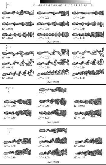
Appendix. Instantaneous flow structures for a transversely rotating sphere at
$\mathit{Re}\ =\ 500$
and
$1000$


The isosurfaces of the vortical structures for the flow past a stationary and transversely rotating sphere at
 $\mathit{Re}=500$
and 1000 are presented in figure 22. (The isosurfaces of the flow structures for
 $\mathit{Re}=1000$
are output to a smaller computational domain compared with those at
 $\mathit{Re}=500$
to minimise computational storage. The simulation computational domain size is of course identical for both Reynolds numbers.) The flow structures are identified using the Jeong & Hussain (Reference Jeong and Hussain1995)
 ${\it\lambda}_{2}$
vortex identification method by plotting an isosurface of
 ${\it\lambda}_{2}=-0.0008$
at the time instant where
 $C_{Ly}$
is at a local minimum.
Instantaneous vortical structures for a transversely rotating sphere at
 $\mathit{Re}=500$
and 1000. The isosurfaces are identified using the
 ${\it\lambda}_{2}$
vortex identification and coloured by the streamwise vorticity,
 ${\it\omega}_{z}$
.

At
 $\mathit{Re}=500$
and
 ${\it\Omega}^{\ast }=0.00$
, vortices are shed from the sphere in random directions. This is consistent with many experimental studies (Magarvey & Bishop Reference Magarvey and Bishop1961; Sakamoto & Haniu Reference Sakamoto and Haniu1990) and numerical simulations (Mittal Reference Mittal1999; Lee Reference Lee2000; Tomboulides & Orszag Reference Tomboulides and Orszag2000; Ploumhans et al.
Reference Ploumhans, Winckelmans, Salmon, Leonard and Warren2002; Bagchi & Balachandar Reference Bagchi and Balachandar2004). Transverse sphere rotation forces vortex loops to roll up in the
 $y$
direction perpendicular to the rotation axis (
 $x$
-axis). The vortex shedding regime exists until
 ${\it\Omega}^{\ast }=0.60$
. At
 ${\it\Omega}^{\ast }=0.80$
, flow is governed by the Kelvin–Helmholtz shear layer instability. The same mechanism has both been discussed qualitatively by Giacobello et al. (Reference Giacobello, Ooi and Balachandar2009) and Kim (Reference Kim2009), and quantitatively compared with the linear stability analysis by Poon et al. (Reference Poon, Ooi, Giacobello and Cohen2013). The flow structures show a chaotic pattern at
 ${\it\Omega}^{\ast }=1.00$
as they enter the ‘shear layer–stable foci’ regime.
For flow past a sphere at
 $\mathit{Re}=1000$
and
 ${\it\Omega}^{\ast }=0.00$
, a shear layer of the Kelvin–Helmholtz instability type can be observed (Kim & Durbin Reference Kim and Durbin1988; Sakamoto & Haniu Reference Sakamoto and Haniu1990; Bonneton & Chomax Reference Bonneton and Chomax1992), and this leads to the formation of the small eddies in the wake (Yun et al.
Reference Yun, Kim and Choi2006). As the sphere rotates, the flow structures are topologically similar to those at
 $\mathit{Re}=500$
and
 ${\it\Omega}^{\ast }\in [0.30,0.60]$
; this clearly shows the periodic roll-up and shedding of large-scale vortex structures together with small-scale vortices in the wake which are released via a Kelvin–Helmholtz instability. These small-scale vortices are a result of the increase in local Reynolds numbers,
 $\mathit{Re}_{l}$
, on the advancing side of the sphere (in the negative
 $y$
direction). On the retreating side of the sphere,
 $\mathit{Re}_{l}$
decreases and thus the Kelvin–Helmholtz instability is suppressed. It is also important to mention that although the induced vortices on the retreating side of the sphere become less pronounced as
 ${\it\Omega}^{\ast }$
increases, they are not completely suppressed in this range of rotation rates. For
 ${\it\Omega}^{\ast }=0.80$
, the flow enters the ‘shear layer–stable foci’ regime. The stable focus increases in size as
 ${\it\Omega}^{\ast }$
increases and leads to a more chaotic flow pattern, as shown in figure 22.