I am taking advantage of the opportunity afforded me by my presidency of the EHA to write what amounts to a personal memoir. It is something of an homage to data for data have been good to me. During my career, I have collected many different data sets; some as a research assistant, others as a principal investigator.Footnote ¹ All have been “hands on” and all have figured in my own research. All have also been public goods.Footnote ² None, however, has attracted quite the interest with as much speed of uptake as my ongoing work to develop a historical transportation database for the United States.Footnote ³ Consequently, I think it important and useful to describe in detail how these data have been assembled and what their virtues and pitfalls might be. In doing so, it is my intent that this description serve as a reference for users. It might also serve as a blueprint for others desiring to do similar work or who wish to extend what I have done.

Widespread interest in transportation is hardly surprising given the importance of transportation improvements in economic growth and development and their role in the historiography of our field. For example, Thomas Jefferson's Secretary of the Treasury, Albert Gallatin, could confidently assert in his report to the U.S. Senate that “the general utility of artificial roads and canals is at this time so universally admitted as hardly to require any additional proofs” in making his case for more and better means of communication within the United States despite the lapse of more than two thousand years since Appius Claudius Caecus began construction of the road that would bear his name (U.S. Congress. Senate and U.S. Department of the Treasury 1808; Della Portella 2004). The case that Gallatin made was a familiar one to contemporaries then, as now. It emphasized the general gains arising from the changes in the cost of transportation which are central to calculations of social savings by Robert Fogel, Albert Fishlow and others (Fogel 1962, 1964; Fishlow 1965). It also emphasized the trade creation and trade diversion effects arising from the removal of trade barriers that, for example, play a central role in Douglass North's model of regional trade and economic growth (North 1955, 1961, 1966).

In the years preceding Gallatin's report, a multitude of transportation infrastructure improvements had been concluded. These included the Charles River Bridge between Cambridge and Boston in 1786; the Philadelphia to Lancaster turnpike which opened to traffic in 1792, and the Santee Canal which passed the first canal barges through its locks between Charleston SC and the Santee River in 1800 (see, for example, United States Supreme Court, Proprietors of Charles River Bridge et al. 1837; Landis 1918a, 1918b, 1918c, 1919a, 1919b; Landis, Webb et al. 1918; Webber 1927a, 1927b; Taylor 1951; Kutler 1971). Despite this flurry of activity, however, the driving force behind Gallatin's plan was the perception that the expansion of transportation infrastructure through private sector efforts alone was too slow and haphazard to meet the economic and the political needs and aspirations (including national security) of the country. As a result, Gallatin advocated for the “early and efficient aid of the Federal government” [emphasis in the original] on the grounds that, “No other single operation, within the power of Government, can more effectually tend to strengthen and perpetuate that Union which secures external independence, domestic peace, and internal liberty” (U.S. Congress. Senate and U.S. Department of the Treasury 1808, pp. 724–25) That role has been extensively investigated and the subject of spirited debate (Fogel 1960; Goodrich 1960, 1961, 1967; Mercer 1969; Duran 2010).

The impact of improvements in transportation upon markets has been illustrated by generations of economic historians using price data for some tradable good. An abundance of such data are to be found in “prices current,” which first appeared in Philadelphia's American Weekly Mercury in 1719, and in New York papers beginning in 1720 (Bezanson, Gray, and Hussey 1935; Cole 1938a, 1938b; Berry 1943). By 1732 similar data appeared for Charleston (Taylor 1932; Warren, Pearson, and Stoker 1932) and, by the early nineteenth century local prices appeared irregularly in Kentucky and Ohio papers. Those Midwestern local prices were also often printed alongside New Orleans prices and those in even more distant markets (Berry 1943, pp. 14–15). The publication of price data reduced any monopsony power that particular groups of traders might have enjoyed. However, such data also have an immediate appeal to economists via the law of one price which posits that, in the absence of trade barriers, savvy traders would exploit arbitrage opportunities by buying in the cheaper market and reselling in the more expensive (Persson 2008). In an open economy with a common currency such as the United States, the major barriers to trade were distance and high transport costs. However, over time as transportation improved both in cost and also in quality dimensions such as speed and the certainty of timely delivery. The impact of these changes has even been described as revolutionary without accusations of hyperbole (Taylor 1951).

Figure 1

PRICE CONVERGENCE IN THE WHEAT MARKET: NEW YORK-CHICAGO, 1841–1910

Sources: Chicago price data: Boyle (1922); New York price data: Ronk (1936).

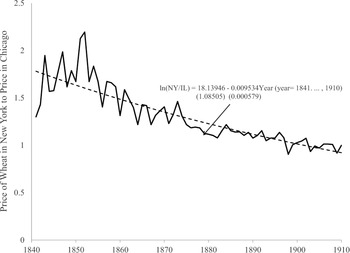
The possible impact of such changes may be illustrated with data on the price of wheat in Chicago and New York from 1841 to 1910 (Boyle 1922; Ronk 1936). These show an increase in the price of wheat in New York relative to Chicago before about 1850 but then there is a steady decline in that ratio from more than 2 to 1 to just about 1:1 by 1900 (Figure 1).Footnote ⁴ Key events bringing about these changes are the improvement in transportation into and out of Chicago beginning with the opening of the Illinois and Michigan canal between Lake Michigan and the Illinois (and thus, the Mississippi) River in 1848 (Conzen and Carr 1988; Cronon 1991). The first railroad arrived the same year but it was not until the arrival of the Michigan Southern Railroad in 1852 that Chicago had connections to the East. Even so, it was not until 1858 that the first all-rail link between Chicago and New York City opened. However, on the eve of the Civil War, the city was served by 11 railroads, allegedly with 100 trains a day (Grossman, Keating, and Reiff 2004, “Transportation,” p. 826ff). Indeed, during the 1850s Illinois became the epicenter of railroads construction in the United States with most of the rails being concentrated in the leading wheat and corn-producing counties (Fishlow 1965).

Figure 2

TRANSPORTATION “WEDGE”: CHICAGO-NEW YORK, 1841–1910

Sources: Chicago price data: Boyle (1922); New York price data: Ronk (1936).

The fitted trend line (the dashed line in Figure 1) shows a statistically significant and reasonably rapid rate of price convergence between Chicago and New York wheat prices averaging about 1 percent per year over the period. Similar rates of price convergence are reported by others (see, for example, Slaughter 1995).

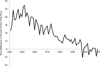
A somewhat different way of looking at these same data is simply to take the difference between market prices in the two markets as a percentage of the price in New York City (Figure 2). Looked at in this way, there is a price “wedge “ between Chicago and New York of between 40 and 50 percent from the mid-1840s through the early 1850s. This wedge then declines sharply to 20–30 percent by the early 1860s where it remains until dropping sharply lower beginning in the mid-1870, plateauing at between 5 and 15 percent from the mid-1880s through the mid-late 1890s before being eliminated (subject to cyclical fluctuations) thereafter.

In their analysis of the various transportation improvements, however, previous generations of economic historians have faced a major challenge in dealing with the locational effects of specific improvements. The location of those improvements provided a point to which distance could be measured and from which influence (market access to and from elsewhere, information flows, etc.) radiated. Adequate modeling tools to deal with this simply did not exist. The famous drawing in Fogel's Railroad and American Economic Growth (1964) showing land in the 48 states that lay within 40 airline miles of navigable waterways in 1890 or those navigable waterways which could have been built, for example, took months to produce.Footnote ⁵ More recently, Lee Craig and Thomas Weiss spent hours poring over old maps trying to map their approximations of navigable waterways and rail lines into contemporaneous county boundaries in 1850 and 1860 (Craig, Palmquist, and Weiss 1998). It was this work more than any other which encouraged and inspired my current endeavors.

Specifically, their efforts motivated me to try harder to understand geographic information systems (GIS) so that I might develop a GIS transportation database for the United States. I am still learning GIS and my work assembling a comprehensive transportation database is still incomplete. Nevertheless, a growing number of scholars are already using my data making it increasingly important that the fundamentals underlying them are understood by audience and researchers alike.

The work by Craig and Weiss was one of several pieces appearing in a special issue of the Journal of Real Estate Finance and Economics which grappled with GIS/spatial location problems (see also Atack and Margo 1998; Coffman and Gregson 1998). Robert Margo and I were certainly frustrated with the spatial tools we had available and our ability to use them. I had long endeavored to use spatial tools from my first encounters with the late geographer Carville Earle (LSU Department of Geography and Anthropology 2004) and with the Great American History Machine which brought the ICPSR county level data together with mapping capabilities and simple analytical tools (Miller and Modell 1988; Miller 1995) and built upon the choropleth maps that began appearing with the 1870 Census (United States. Census Office., Walker et al. 1874). I had early copies of DOS-based software like “Atlas Graphics” from Strategic Locations Planning Inc. of San Jose. The work of others, notably Anne Knowles (Knowles 2002) and Richard Healey (Waugh, Healey et al. 1995; Healey and Stamp 2000; Healey 2007), however, also pointed the way forward. Knowles’ book, in particular, illustrates the diversity of historical issues on which GIS can shed new light from the Salem Witch trials to Civil War battlefields to the Dust Bowl of the 1930s.

My initial effort to improve upon Craig and Weiss (1998) was a miserable failure. I began with the digitized maps available through the Library of Congress “American Memory” website. The earliest map showing railroads is by Henry Tanner and dates from 1830 (Tanner 1830). It shows a number of railroads as operational—certainly more miles than were actually operational at that time. For example, it shows an operational rail link between Harpers Ferry and Winchester, the Winchester and Potomac Railroad, although that route was not surveyed until 1831/32 (Haney 1968) and did not open until 1836 (Dilts 1993, p. 191). Indeed, the Baltimore and Ohio Railroad to which it would link did not itself reach Harpers Ferry until 1834 (Stover 1987; Dilts 1993). Similarly, Tanner's map shows the Columbia-Philadelphia Railroad as operational although it did not see its first train until 1832 (Wilson 1985). Consequently, I began my foray into GIS with David Burr's (credentialed on the map as “geographer to the House of Representatives of the U.S.”) (Burr 1839) map from 1839. I then moved on to later years such as Disturnell's map for 1851 (Burr 1851), and Colton's maps for 1860 and 1870 (J. H. Colton 1860; G. W. Colton 1870).

At some point, however, I began to reexamine my series of mappings and quickly realized that because of the inaccuracy of the underlying maps, the collection did not work as a time series even if the individual renderings were useful. Specific railroads “changed” location from map to map. Some magically disappeared only to reappear in later mappings. I should have realized problem before I began. It was right there in front of me with the early Tanner and Burr maps (Tanner 1830; Burr 1839). The operational nature of some railroads was a figment of the cartographer's imagination (or faulty information). Indeed, Mark Ovenden (2011) even has a clever word for it: “cartograFibs.” Moreover, the railroads themselves were drawn with the early nineteenth-century equivalent of a magic marker and in the manner not unlike that which child might use if asked to connect point A to point B.

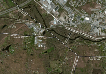
I began again. This time my efforts were more successful thanks to a reversal in strategy. Rather than moving forwards in time, I would go backwards. I began with a set of fairly accurately drawn, state-level, digitized maps available on CD from http://www.goldbug.com under the title “Historic Map Library: 1911 Century Map series-Eastern United States” and “Historic Map Library: 1911 Century Map series-Western United States.”Footnote ⁶ Their dating predates by a few years the maximum railroad track mileage in the United States (Carter et al. 2006, Series Df930-933).Footnote ⁷ Since then, about 100,000 miles of track have been torn up. My assessment that the 1911 maps are fairly accurately drawn rests on a simple comparison of the location of railroads still in operation (United States Department of Transportation. 2012) (but which may have been realigned) and those in 1911. An illustration of the mapping accuracy based upon the 1911 maps is shown in Figure 3 for the southern fringes of Willimantic, Connecticut. The heavy dot-dashed white line is the railroad today as traced in the National Transportation database (United States Department of Transportation 2012) from a satellite image such as that which it overlies. The heavy black and white dashed lines represent the railroads mapped in 1911 from the map for Connecticut (Whitney and Smith 1911). The distance between the railroad location as mapped in 1911 and where it actually lies is a matter of a few hundred meters on the ground.Footnote ⁸ In 1911 more railroads passed through Willimantic than do today. In just the area shown, two lines were torn up sometime after 1911. However, faint vestige of those missing lines may still be seen from the shape of property lines, vegetation, and buildings (and as indicated by “Abandoned railroad” and an intermittent trail of white dot “bread crumbs” that I placed on the image).Footnote ⁹ To trace the 1911 rail system, I digitized “only” 145,000 points. To map the 238,000 miles of railroad track shown in the National Transportation Atlas database, more than 1,380,000 points were digitized, or more than 9 times as many points as I used.Footnote ¹⁰ Not surprisingly, the National Transportation database features drawn from satellite imagery follow railroad lines more closely than do my 1911 tracings. I will return to this general point later.

Figure 3

WILLIMANTIC, CONNECTICUT: RAILROAD LOCATION TODAY FROM SATELLITE IMAGERY AND RAILROAD LOCATIONS AS MAPPED IN 1911

Source: Mappings from author.

Moving from a digitized image of a map to a GIS database requires several steps. The following steps are those that one would take using ESRI's ArcGIS software which generates a series of interlinked and interdependent files that I am referring to collectively as a GIS database.Footnote ¹¹ The first step is to “geo-reference” the digitized image by providing spatial coordinates. These will provide the means to relate this image to others. In my specific example, I use a geographic coordinate system and these spatial coordinates are provided by reference to a boundary shapefile and transferred to the digitized map through a process aptly described by many as “rubber sheeting.”Footnote ¹² Conceptually, this involves pinning a specific, easily identified point from the digitized image to the corresponding reference point on the boundary file. I used points such as where several state (or county) boundaries meet. This process is then repeated for other fixed points and, in essence, the digitized image is stretched as if drawn on a sheet of latex rubber, distributing the interval evenly between the fixed points so that the digitized image more or less perfectly overlays the boundary file. With a well-drawn, accurate map, relatively few points—at least two but four generally worked well with the 1911 state maps—are needed. If, however, the map is distorted in some way, more points are needed to make for an acceptable fit (determined by the user) between the digitized image and the boundary file.Footnote ¹³ In ArcGIS, this geo-referenced image is then rewritten—“rectified”—so that it may be reused in whole or in part with related boundary files at any scale or magnification as a layer. One great advantage of electronic GIS over paper copy is the ability to render any layer transparent to any desired degree and so to overlay such images on top of one another. One can therefore immediately see whatever features that one desires in whatever layer with the correct spatial relationships one to another. As a result, one also has immediate access to modern cartographic resources—satellite imagery, topographical maps from the U.S. Geological Service, and even hybrid BING maps from Microsoft which merge satellite imagery with highway maps and the like—which overlay as “Base Maps” in ArcGIS v.10 and align with any correctly georeferenced feature file created as described above.

Once one has a spatially linked image to work with, tracing features from the digitized image into a shapefile simply requires the creation of a new feature database of the correct type and the digitization of appropriate points. Features can be points, lines or polygons. A point is simply that, a single point. Lines are created by the GIS software connecting two or more points together. Polygons are created by the software by connecting consecutive polygon vertices with lines and then closing the polygon by connecting the last point to the first point.Footnote ¹⁴

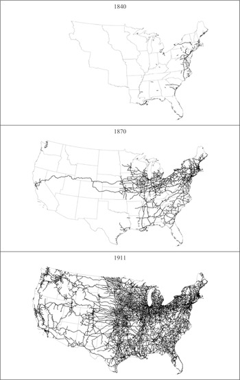
To create a mapping of railroads for dates prior to 1911, I began with a copy of the shapefile for the next later year (so, for example, the mapping for 1887 used a copy of the 1911 railroad shapefile as a starting point, while the 1882 mapping was based upon a copy of the 1887 shapefile). I then overlaid the copy on the geo-referenced and rectified digital map showing the railroad system for the year I desired. Not surprisingly, the railroad lines shown on an earlier map did not perfectly align with the digitized tracings from the later map. However, the fit is sufficiently close that one can confidently erase railroad lines and line segments—by entering editing mode, selecting the erroneous tracings and deleting those where no line appears on the earlier map (making due allowance for imperfections in the overlay). The end product is a series of perfectly coincident railroad lines, whose location is fixed in its 1911 place but whose extent reflects the extent of that line at some earlier date (Figure 4). Fading one feature into later features generates the movie of the spreading railroad network shown at http://journals.cambridge.org/action/displayJournal?jid=JEH (under “JEH Railroad and Waterways Maps”). Thus far, I have railroad mappings covering the lower 48 states for 1830, 1840, 1851 (Burr 1851), 1860 (J. H. Colton 1860), 1870 (G. W. Colton 1870), 1882 (G. W. Colton 1882), 1887 (Cram 1887), and 1911 (Whitney and Smith 1911). The choice of dates from 1851 onward has been dictated by the availability of what I view as suitable maps on the Library of Congress “American Memory” website and elsewhere. There is, however, an abundance of other sources of high-quality digitized images including the David Rumsey map collection (now housed at Stanford University) and public and university libraries (for example, http://www.lib.utexas.edu/maps/historical/index.html). The mappings prior to 1851 were based upon a database of early railroads operating in the United States assembled by Professor Milton C. Hallberg (1936–2012) and available online at www.oldrailhistory.com modifying my 1851 mapping as necessary.Footnote ¹⁵

Figure 4

THE AMERICAN RAIL SYSTEM AT BENCHMARK DATES

Source: GIS mappings from Atack, Jeremy. National Historical Transportation Database (as of January 2012) on state-level NHGIS boundary files from http://www.nhgis.org.

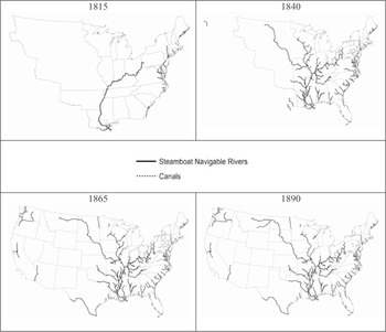
The railroad mappings represent just one dimension of my transportation database albeit the one which has attracted the greatest attention to date. I have also assembled information on canals and rivers.Footnote ¹⁶ Several sources provided information about the construction of canals during the nineteenth century. These sources include Henry Poor (1970) and Carter Goodrich (1961). Maps in these sources as well as in the Library of Congress “American Memory” collection (see, for example, Tanner 1830) also provide indications of the approximate location of the canals. More precise locations for each canal have been determined based upon topographical maps and histories of the individual canal projects. Many of these histories are available online (see, for example, http://www.winchestermass.org/canal.html for the Middlesex Canal) and they provide useful information about the construction of specific sections of canals and when these were opened to traffic and also when they were abandoned.Footnote ¹⁷ As a result, it has been possible to generate a year-by-year mapping of the canal system in America such as has thus far proved elusive for the rail system.Footnote ¹⁸

The canal system sometimes made use of stretches of navigable river but the canals themselves are generally well-defined. The notion of a navigable river, however, is much less clear cut.Footnote ¹⁹ Canoes could and did travel on almost any river, stream, or lake. However, while a canoe can hold several hundred pounds of cargo and bateaux carried several tons, I have taken commercial shipping to involve something larger and more technologically advanced.Footnote ²⁰ Specifically, I have tried to determine where and when steam navigation became a normal part of life. This definition of a navigable river is narrower than that used by Fogel's (1964). The differences are especially great in the South. For example, according to a history of Conecuh County, Alabama, one steamboat, the “Shaw,” managed to steam upriver as far as the town of Brooklyn in 1845/46, but it sank almost immediately upon starting out on its return voyage, putting an abrupt, and early end to steam navigation of the Conecuh and Escambia Rivers (Riley 1881).Footnote ²¹ The mapping of navigable rivers was taken from U.S. Army Corp of Engineers GIS data (Vanderbilt University. Engineering Center for Transportation Operations and Research 1999). The dates attached to steamboat navigation of the rivers come from Louis Hunter (1949), gazetteers (for example, Rowell 1873), contemporary newspaper accounts regarding steamboat service on specific rivers found through online searches, and searches of congressional reports (see, for example, U.S. Congress. House, Engineers et al. 1871, p. 12).Footnote ²² Like the canal database, the river database effectively shows the expansion of inland water navigation on an annual basis (Figure 5). Collectively, these data suggest that river and canal navigation in the United States increased from about 300 miles in 1800 to over 10,000 miles by 1826, more than 20,000 by 1841, and over 25,000 miles by 1860. The river and canal system peaked in the late 1870s at about 26,000 miles but, by then, canals had been on the wane for more than a decade and water waterways in general had been eclipsed in terms of mileage by railroads by the late 1850s. A time-lapse “movie” of the spread of river navigation by steamboat and canals during the nineteenth century is available at http://journals.cambridge.org/action/displayJournal?jid=JEH.

Figure 5

RIVER STEAMBOAT AND CANAL NAVIGATION AT BENCHMARK DATES

Sources: See the text for a description of transportation series. State boundary outlines are from state boundary files from www.nhgis.org. Those underlying 1815 are for 1820 and those underlying 1865 are for 1870. State boundaries in 1840 and 1890 are as shown.

My GIS skills, such as they are, have relied heavily upon personal training that I received from a GIS expert, Jacob Thornton, whom Vanderbilt University had presciently hired to the library staff despite Vanderbilt not having a geography program. Jacob proved to be an invaluable resource and he would serve as a catalyst for many GIS projects around campus. I describe him accurately as “invaluable” since, despite having had GIS software of one flavor or another for at least fifteen years, I had found successive generations of GIS software all but impenetrable. Even with Jacob's help, my learning curve on ArcGIS has remained depressingly flat. The ArcGIS software is enormously complex and has its own vocabulary.

Figure 3 which compared my GIS mapping based on printed maps from 1911 with that from current satellite imagery suggests several sources of error. The original maps may be wrong. The mapmaker, for example, may have had less than perfect information about the location of new railroads as, for example, was the case with the crudely drawn lines in Henry Burr (1839). Railroad builders may have been over-optimistic in their estimate of the construction speed and prowess and mapmakers seeking to maximize their usefulness and longevity of their product tended to be forward-looking (see, for example, Tanner 1830). A financial crisis may have interrupted the flow of funds needed to complete an otherwise certain project. Nor is it unheard of for a mapmaker to deliberately include errors in his map in order to detect illegal copying. Errors also arise in the creation of the shapefile. The digitized map may have been poorly geo-referenced. That geo-referenced map may have been imperfectly traced. In short, errors can and do occur throughout the process; the system is far from perfect. Nevertheless, it remains better than trying to determine the location and extent of a transportation network by eye.

A careful study of satellite imagery (see, for example, Figure 3) suggests that even when features like railroad lines have been torn up and nature has tried to reclaim that right of way, traces still remain.Footnote ²³ Railroad ballast, for example, was designed for drainage so even when crops now grow atop old railroad rights of way, growth patterns and vegetation coloration still often give its presence away. So too do cuts and fills. Even more helpfully, the legend “Old Railroad Grade” sometimes appears on current topographical maps.Footnote ²⁴ Occasionally, however, evidence of an abandoned right of way was totally obliterated when it was incorporated into a new road as was the case with some former Union Pacific right of way which is now a part of the Interstate 10 (I-10)/Katy Freeway outside of Houston. Nevertheless, it may ultimately prove possible, using the 1911 mappings as a guide and current satellite imagery as a starting point, to recreate a mapping of railroads for the early twentieth century that has the accuracy of location inherent in satellite mapping but which truly captures the extent of America's railroads in 1911.

The mappings that I have made thus far only trace the location of transportation media during the nineteenth and early twentieth century. Other features and attributes, however, are important. It is, for example, tempting to refer to the railroad system as a “network,” ignoring the fact that many different and incompatible track gauges were in use before the United States settled on the standard (4 feet 8½ inches) gauge system (Puffert 1991, 2000). Until that standardization took place, the interchange of cargo between different railroads often required unloading and reloading. Even neglecting the practical issue of track gauge, it is not possible to switch from one railroad line to another with the current GIS mapping even when those lines cross unless that intersection marks the end or beginning of a line segment. Where this is not the case, it is as if one railroad track flies over the other as on a bridge. This is an artifact of GIS and a result of decisions that I made when digitizing the 1911 data.Footnote ²⁵ Each line segment that I digitized began and ended at a named place on the 1911 maps—likely a station or depot but certainly a place worthy of note and thus a place where interchange might occur. Such “Wye” (or “Y”) interchanges required points and someone to operate (and reset) those switches. That operator might be the engineer/conductor on the train, in which case the train had to at least slow to a crawl, if not stop, when passing through, or the switches might be operated by a dedicated railroad employee stationed there for exactly that purpose. However, the scale of the underlying maps that I use is such that minutiae regarding track configurations are unobservable.Footnote ²⁶

Stations and depots provided a focus for economic activity through the routine pickup and drop off of freight and passengers, although at earlier times trains might stop almost anywhere to pick up or drop off, just as the flag stop service on the Alaska Railroad does today. The earliest railroad map for the United States that I have found which explicitly lists depots and stations is from 1856 (Ensign 1856). Thereafter, stations and depots are marked on maps with increasing frequency (Sage 1858). Indeed, many cartographers begin to advertise their works as “commercial” maps (see, for example, G. W. Colton 1870). Recognizing the importance of this kind of information, Rand McNally began to publish a series of commercial Atlases beginning in the 1870s (Library of Congress. Geography and Map Division and Modelski 1975). These served the needs of shippers by advising them to which station goods should be consigned. Such maps also served the interests of commercial travelers who rode the rails from town to town in the manner shown in the opening scene of “Music Man.” However, even where maps marked cities with railroad stations, not all railroads went to the same station or depot in that city. This further complicated the interchange of traffic and the treatment of railroads as a network. The construction of “Union Stations,” beginning with that in Indianapolis in the early 1850s (see http://www.nps.gov/nr/travel/indianapolis/unionstation.htm), was a giant step towards resolving this problem although the movement nationwide did not really catch fire until the 1890s and continued into the 1930s (Chappell 1989).Footnote ²⁷ Other railroad specific information can also be linked to the GIS transportation database such as the information regarding fares and travel times that appears in the numerous contemporary travel guides (see, for example, Appleton; Disturnell 1847; Doggett 1848; Cobb 1853; Lloyd 1857; Rand McNally and Company, National General Ticket Agents’ Association et al. 1879).Footnote ²⁸

This historical GIS transportation database will change our understanding of the contribution made by transportation improvements to American economic growth and development. Most of the analysis with which I have been involved thus far uses a GIS rendition of Frederic Paxson's (1914) data for the Old Northwest, expanded to include Iowa and Missouri, to measure the effect of the coming of the railroad using a difference-in-differences framework with an instrumental variable as a robustness check. The argument for focusing attention on the Midwest is that this was the region that saw the most dramatic expansion of the rail system in the 1850s (Fishlow 1965). That expansion also coincides with the collection of vastly more economic and social data as a part of the increasing scale and scope of the federal census (Wright 1900). To date, waterborne transportation plays the role of a control in our modeling. Using county-level data for those counties whose borders remained unchanged throughout the period, we (Atack et al. 2010) found that the railroad accounts for more than half of the increase in urbanization in the region (and primarily through its effects upon the growth of many smaller towns and cities throughout the region rather than by its effect on the growth of a few large centers) even though its effect upon population growth per se seems to have been minimal. If and when more detailed population data become available for the United States at the township and town level, one might see more effect upon location-specific population growth as, for example, Marta Felis, Jordi Marti Henneberg, and Laia Mojica (Felis-Rota, Henneberg, and Mojica 2012) find in England and Wales using parish level population data relative to railway lines and stations. In the United States, such urban growth was, in turn, central to the expansion of manufacturing, trade and commerce, and productivity growth (Kim 1995, 2000; Atack, Bateman, and Margo 2004, 2005).

Areas of the Midwest served by rail also saw land values rise much more rapidly than in other areas lacking such transportation access. In those places, farmers cleared more land and planted more crops. Indeed, we attribute as much as two-thirds of the increase in improved acreage in the Midwest in the decade before the Civil War to the spread of the railroad in the region (Atack and Margo 2011). Those rising land value also made it more difficult for persons to become land owners at a time when capital markets were imperfect and still developing thus potentially slowing the ascent of farmers up the agricultural ladder (Atack and Margo 2012).

One key component in the evolving capital markets was the role played by financial intermediaries, especially banks. In other, more preliminary work with Matthew Jaremski and Peter Rousseau (Atack, Jaremski, and Rousseau 2013), we find that counties which already had a bank were more likely than others to see the railroad come during the next decade, and that new banks tended to enter a county a year or two after it got a railroad. This pattern suggests that early banks in a county helped to establish the rail system while the rapid development of railroads thereafter helped fill in the banking map at least so far as the American Midwest was concerned.

The effect of the railroad, however, was not confined to the American Midwest or to the antebellum period. We have found that rail access was positively and significantly associated with the location of inanimately powered, larger manufacturing establishments (Atack, Haines, and Margo 2010). Such businesses made much more extensive use of the division of labor and specialized capital goods than smaller establishments. As a result, they were productivity leaders and they formed the nucleus around which American manufacturing rose to dominance in the late nineteenth and early twentieth centuries (Wright 1990; Broadberry and Irwin 2006).

Moreover, the effects of the improved transportation also show up in human capital formation where preliminary work suggests it may account for perhaps 40 percent of the observed increase in school attendance between 1850 and 1880 (Atack, Margo, and Perlman 2012). Lastly, I would note the conclusion of Dave Donaldson and Richard Hornbeck (2012) based upon their analysis of post-Civil War changes in market access from the spread of the railroad that Fogel (Fogel 1964) may significantly underestimate the railroad's social saving. Although it is, as yet, too soon to (re-) assert the indispensability of the “iron horse” for American economic growth and development, it is not too soon to claim that historical GIS transportation databases will change our interpretation of American economic history.