1 Introduction
In the late 1980s – in concert with an increase in the number of blades being used in aerospace propeller designs – researchers began to use a high-blade-number asymptotic approach to study and understand propeller noise. Parry & Crighton (Reference Parry and Crighton1989a ) showed that subsonic propeller noise could be predicted using a simplified formula that removed the need for an integration over the blade span, and showed how the noise is dominated by radiation from the blade tips, with the result linked precisely to the tip geometry. Crighton & Parry (Reference Crighton and Parry1991, Reference Crighton and Parry1992) applied the approach to supersonic propellers where the noise is dominated to leading order by radiation from a sonic radius with a lower-order term arising from the blade tips; the leading-order term is purely an algebraic expression. For swept propellers Parry (Reference Parry1995) applied asymptotics in the frequency domain to a two-dimensional source annulus to show that the noise is dominated by regions (critical points) in which (a) the blade leading edge is moving at precisely sonic speed in the direction of the observer and (b) the blade leading edge is normal to a position vector from the observer to the blade leading edge; these criteria had previously been obtained in the time domain by Amiet (Reference Amiet1988). Whilst straight-blade propellers have, at most, a single critical point, Parry (Reference Parry1995) showed that, for a swept propeller, the noise could be increased relative to a straight propeller due to the presence of multiple, or continuums of, critical points. Other applications of high-blade-number asymptotics have been made to near-field propeller noise by Peake & Crighton (Reference Peake and Crighton1991a ), to propeller quadrupole noise by Peake & Crighton (Reference Peake and Crighton1991b ), and to reduce computation time for propeller noise calculations by Envia (Reference Envia1994), who maintained a high-fidelity calculation of the local source region that ensured the result naturally applied to both far and near fields and to loading, thickness and quadrupole source terms. Also of interest are the time-domain analyses of propeller noise by Chapman (Reference Chapman1992) and Prentice (Reference Prentice1994a ,Reference Prentice b ). Those authors did not explicitly use high-blade-number asymptotics and opted, instead, for asymptotically small blade chord. Nonetheless, since blades are usually designed with fixed space/chord (or pitch/chord) ratio (see, for example, Saravanamuttoo et al. (Reference Saravanamuttoo, Rogers, Cohen, Straznicky and Nix2017)), it follows that small chord is equivalent to large blade number.
To the authors’ knowledge, there has been little work on the application of asymptotic analyses to contra-rotating propellers. Envia (Reference Envia2015) extended previous work on single-rotating propellers to the contra-rotating case, with the radiation expressions, as before, requiring a high-fidelity calculation of the local source region. Kingan & Parry (Reference Kingan and Parry2019) extended the two-dimensional surface asymptotic approach of Parry (Reference Parry1995) to study convected wake interactions on contra-rotating propellers, including the effects of blade sweep and sub- or super-critical wake–blade interactions. The analyses produced simplified, largely algebraic, results and showed that the noise is dominated in most cases by localised critical points on the surface of revolution described by the rear blade leading edges. In certain cases – dependent on blade sweep and the order of the circumferential spinning mode – radial or azimuthal one-dimensional continuums of critical points can be present or, exceptionally, a two-dimensional continuum of critical points. Kingan & Parry (Reference Kingan and Parry2019) validated their asymptotic approach extensively by comparing their results with full numerical calculations – of a real engineering test case – over a range of combination frequencies and azimuthal modes, including the zero-mode case, and for both straight and swept propeller blades. For all cases, there was good agreement between the asymptotic results and the numerical calculations (that had, themselves, been validated via many previous comparisons with a wide range of experimental data), showing that the asymptotics could be applied to prediction and design.
The power of the asymptotic analysis in Kingan & Parry (Reference Kingan and Parry2019) lies not just in the accuracy of the results but also in the fact that the formulae indicate precisely how the radiation is linked to certain key regions of the blade, and also to the geometry of the blades in those regions. However, unlike the work of Parry (Reference Parry1995) it did not provide an explanation of why those specific critical regions dominate the sound radiation in terms of the underlying physics; it merely provided a simple equation through which those critical points could be determined. Here, then, our aim is to interrogate Kingan & Parry’s (Reference Kingan and Parry2019) results to help understand the physics of the noise generation and propagation processes associated with those critical regions.
First, though, it is important to be clear about what our approach does and does not do. There is substantial discussion in Kingan & Parry (Reference Kingan and Parry2019) of the assumptions that underpin both the analytical analyses of Hanson (Reference Hanson1980), Parry (Reference Parry1988) and Parry & Crighton (Reference Parry and Crighton1989b ) and the high-blade-number asymptotics, as well as of the alternative computational approaches that can be used for more complex flows. However, we add a little extra discussion here for clarity.
The wakes in Kingan & Parry (Reference Kingan and Parry2019) are generic blade-generated distortions that are convected with the mean flow, and the model can thus be applied to either the viscous or the vortex wake components (including a vortex wake that has rolled up into a tip vortex) but not to the bound potential field components; for the latter it is important to note that, as the distortions are not convected by the mean flow, the rear blade interaction with a potential distortion occurs at a different circumferential location to that of the blade interaction with a convected wake.
The work described here is intended to be applicable in the far field of a contra-rotating propeller at typical take-off or approach conditions, and thus to be relevant to the problem of community noise rather than that of near-field cabin noise. At higher blade speeds – typically relevant to operating conditions at cruise – the noise radiation tends to become dominated by high-amplitude rotor-alone tones caused by steady loading, blade thickness and quadrupole effects. Suitable asymptotic approaches in these areas are Peake & Crighton (Reference Peake and Crighton1991a ,Reference Peake and Crighton b ) and Parry (Reference Parry1995), though we emphasise that the study in this paper is limited to subsonic blade speeds, wake interaction and to far-field noise radiation. (The distances at which the far-field approximation becomes valid for propellers are discussed by Peake & Boyd (Reference Peake and Boyd1993)). The unsteady response of the downstream blades is calculated assuming that they can be represented by flat plates, and the authors have used a modification of Adamczyk (Reference Adamczyk1974) for this purpose. Extensions to account for aerofoil incidence, camber, mean loading, transonic flow and non-uniform mean flow are discussed by Myers & Kerschen (Reference Myers and Kerschen1995, Reference Myers and Kerschen1997), Peake & Kerschen (Reference Peake and Kerschen1997) and Evers & Peake (Reference Evers and Peake2000, Reference Evers and Peake2002), and it may be possible to utilise these analyses to extend the range of applicability of the present paper. For more complex flow fields or for supersonic unsteady interactions, a computational approach is more likely to be necessary (see, for example, Brandvik, Hall & Parry (Reference Brandvik, Hall and Parry2012)).
Finally, the paper is limited to studying the role of blade sweep on the physics of the wake interactions. The effects of lean are neglected. Lean can be aerodynamic or geometric, or both. Aerodynamic lean is a natural by-product of the loading on the propeller and is caused by the presence of swirl, behind the front propeller blades, which convects the wakes circumferentially, as well as axially, such that the wakes become more skewed (circumferentially) with downstream distance – the amount of skew is dependent on the radial swirl gradient. Geometric lean refers to the local dihedral that is produced in the design of realistic propeller blades. In this paper, the approach is based on the helicoidal surface theory of Hanson (Reference Hanson1980, Reference Hanson1985), in which the effects of flow swirl (wake lean) are neglected. The Hanson (Reference Hanson1985) framework has been applied widely and, moreover, has received much validation against experimental data (see the discussion in Kingan & Parry (Reference Kingan and Parry2019)), making it an ideal model for exploitation. Nonetheless, further improvements that could be made to the wake models to make them more realistic are described by the hybrid framework of Ekoule et al. (Reference Ekoule, Kingan, McAlpine, Sohoni and Parry2015, Reference Ekoule, McAlpine, Parry, Kingan and Sohoni2017) and could, with some extensions, be applied to the approach described here. The other important effects relating to lean are those of the unsteady response of the downstream row and of the acoustic radiation. For the downstream blade response it is possible to use, and extend, the work of Graham (Reference Graham1970), Adamczyk (Reference Adamczyk1974) and Glegg (Reference Glegg1999) to account for both aerodynamic and geometric lean (indeed, those approaches can be used even when the inter-row region has a non-zero radial flow component). In addition, circumferential blade lean is included in the fundamental analysis of Hanson (Reference Hanson1985), which describes the acoustic radiation based on the precise location of the unsteady blade forces. However, these lean effects were not included in the asymptotic analysis of Kingan & Parry (Reference Kingan and Parry2019); nonetheless, we point out that these complicated effects, as well as those of potential interactions – both of which exhibit a number of physically interesting phenomena in their own right – could be included in the high-blade-number asymptotic analysis and, thereby, in the implications for the event line discussed in this paper.
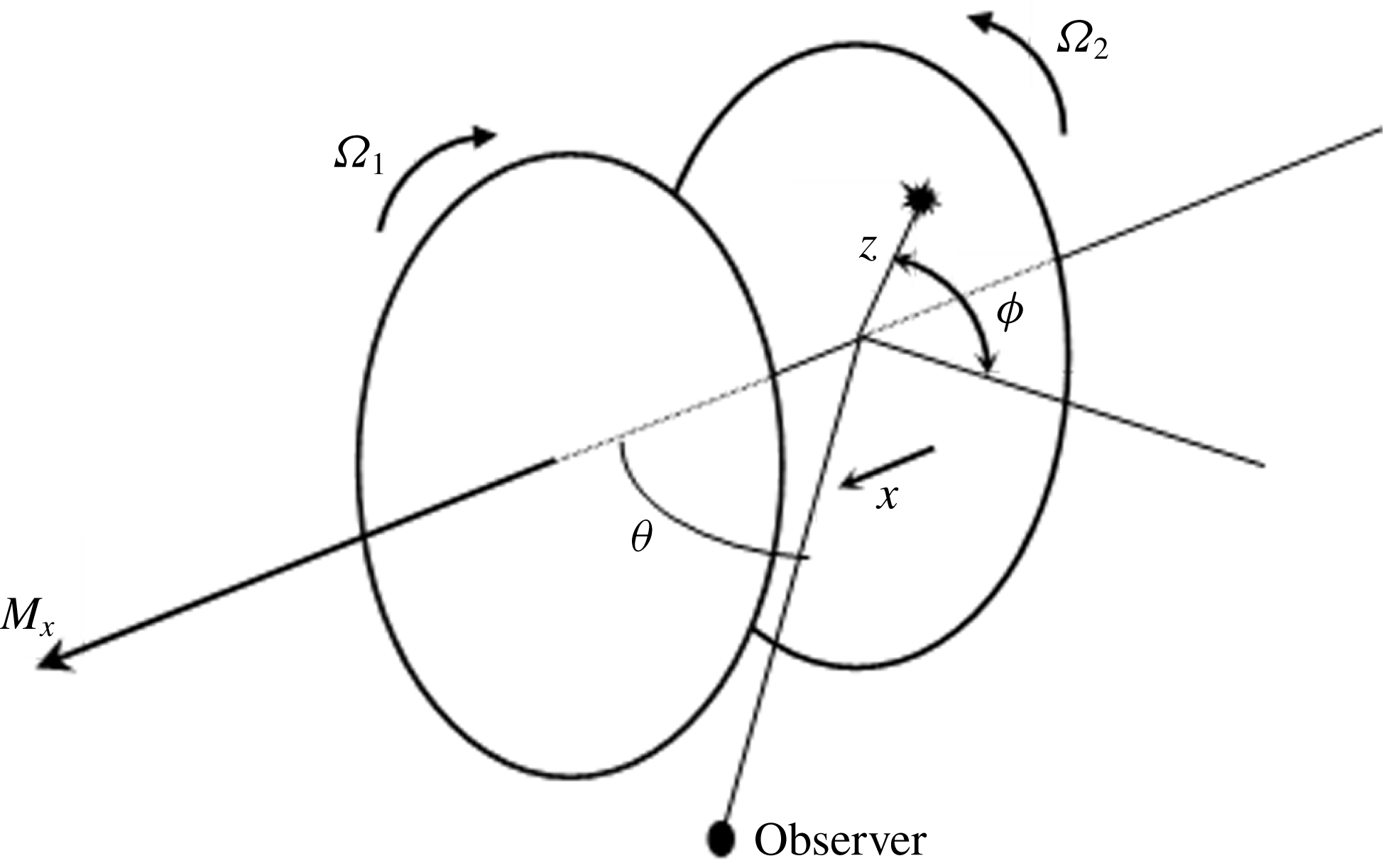
Illustration of the propeller coordinate system.

2 The asymptotic solutions
In order to allow easy comparison with the results of Kingan & Parry (Reference Kingan and Parry2019) we will, in the main, use their notation, which is summarised in this section. The architecture involves two rotating frames, and one absolute frame, as well as important reference points such as the front rotor wake, the rear blade leading edge and the two propeller pitch change axes, and it will be necessary to use all of these frames and locations. The analysis uses a cylindrical coordinate system,
 $(x,z,\unicode[STIX]{x1D719})$
, where
 $x$
is the axial coordinate, which is parallel to the propeller axis,
 $z$
is the radial coordinate and
 $\unicode[STIX]{x1D719}$
is the azimuthal angle. The coordinate system is shown in figure 1. Subscripts 1 and 2 denote parameters associated with the upstream and downstream rotors, respectively, and subscripts
 $x$
,
 $t$
and
 $r$
are used for the Mach numbers in the axial, rotational (at the tip radius) and helical (at radius
 $z$
) directions, respectively. In particular, the rotors move with Mach number
 $M_{x}$
in the positive
 $x$
direction; the upstream and downstream rotors rotate in the negative and positive
 $\unicode[STIX]{x1D719}$
directions with tip rotational Mach numbers
 $M_{t_{1}}$
and
 $M_{t_{2}}$
, respectively; and, for each row,
 $M_{r}=\sqrt{M_{x}^{2}+z^{2}M_{t}^{2}}$
is the section relative, or helicoidal, Mach number. The propeller blades have leading-edge sweep
 $s(z)$
measured from the pitch change axis and each row has
 $B$
blades with front and rear pitch change axes separated by a distance
 $g$
in the axial direction. The observer lies in the
 $\unicode[STIX]{x1D719}=0$
plane at polar angle
 $\unicode[STIX]{x1D703}$
from the
 $x$
axis. For convenience, distances have been normalised on the tip radius
 $R$
, velocities on
 $c_{0}$
and time on
 $R/c_{0}$
, where
 $c_{0}$
is the speed of sound.
For a contra-rotating propeller the radiated tones can be described as a double Fourier series of combination tones
 $(n_{1},n_{2})$
at frequencies
 $\unicode[STIX]{x1D702}=n_{1}B_{1}M_{t_{1}}+n_{2}B_{2}M_{t_{2}}$
and with azimuthal order
 $\unicode[STIX]{x1D708}=n_{2}B_{2}-n_{1}B_{1}$
. As the results depend on the Fourier indices
 $(n_{1},n_{2})$
, they will be retained as subscripts in what follows, where appropriate, to indicate phase terms that are functions of
 $(n_{1},n_{2})$
. Other important parameters used by Kingan & Parry (Reference Kingan and Parry2019) for each of these
 $(n_{1},n_{2})$
combination tones are the non-dimensional radius
 $$\begin{eqnarray}z^{\ast }=\frac{(1-M_{x}\cos \unicode[STIX]{x1D703})}{\sin \unicode[STIX]{x1D703}}\frac{(n_{2}B_{2}-n_{1}B_{1})}{(n_{1}B_{1}M_{t_{1}}+n_{2}B_{2}M_{t_{2}})},\end{eqnarray}$$
which was first introduced for both single-rotating and contra-rotating propellers by Parry (Reference Parry1988), and the sweep factor
 $$\begin{eqnarray}\unicode[STIX]{x1D6E4}(z)=\frac{1}{z^{\ast }\sin \unicode[STIX]{x1D703}}\frac{s}{M_{r_{2}}}+\frac{n_{1}B_{1}}{(n_{2}B_{2}-n_{1}B_{1})}g\frac{M_{t_{1}}}{M_{x}}.\end{eqnarray}$$
Kingan & Parry’s asymptotic analysis showed that as
 $B_{1},B_{2}\rightarrow \infty$
the radiated sound field is dominated, to leading order in
 $\unicode[STIX]{x1D708}$
, by small regions – corresponding to the interior stationary points of the radiation integral – which are localised around radii
 $z$
satisfying
 $$\begin{eqnarray}(z/z^{\ast })^{2}-1=[z\unicode[STIX]{x1D6E4}^{\prime }(z)]^{2}.\end{eqnarray}$$
Additional lower-order solutions came from two boundary points at the propeller hub
 $z_{h}$
and two at the tip
 $z_{t}$
lying at the azimuthal locations
 $u$
satisfying
 $$\begin{eqnarray}u_{+}=\sin ^{-1}(z^{\ast }/z_{b}),\quad u_{-}=\unicode[STIX]{x03C0}\text{sgn}(z^{\ast })-\sin ^{-1}(z^{\ast }/z_{b}),\end{eqnarray}$$
where we have used
 $z_{b}$
to indicate a boundary radius so
 $z_{b}=z_{h}$
or
 $z_{b}=z_{t}$
.
In what follows, other subscripts of note, relating to specific geometric locations, are
 $LE$
,
 $PCA$
,
 $W$
and
 $ev$
, representing the rear blade leading edge, the propeller’s pitch change axis, the front wake’s centreline and an interaction event, respectively. For the Mach number of the pressure disturbances, produced by the interactions, we have also used the subscripts
 $p$
and
 $obs$
for the components in the azimuthal and observer directions, respectively.
3 Physical interpretation of the asymptotic solutions
3.1 Interaction event
We use
 $\unicode[STIX]{x1D719}_{2}=\unicode[STIX]{x1D719}-M_{t_{2}}t$
to switch to a frame of reference rotating with the downstream propeller, and follow the approach of Tyler & Sofrin (Reference Tyler and Sofrin1962), who showed that the pressure disturbance anywhere ahead of or behind the blades, and at an arbitrary radial height, can be written – in our notation – as a function of azimuthal location
 $\unicode[STIX]{x1D719}_{2}$
and time
 $t$
in a double Fourier series of terms
 $p_{n_{1},n_{2}}\cos [(n_{1}B_{1}-n_{2}B_{2})\unicode[STIX]{x1D719}_{2}-n_{1}B_{1}(M_{t_{1}}+M_{t_{2}})t+\unicode[STIX]{x1D712}_{n_{1},n_{2}}]$
, where the series is summed over positive values of
 $n_{1}$
and positive and negative values of
 $n_{2}$
.
Tyler & Sofrin (Reference Tyler and Sofrin1962) referred to the space-time interaction between a front rotor wake and a downstream stator leading edge as a blade-vane event or, more simply, as an event. In order to study the variation in the blade-vane event with radius we now allow the amplitude
 $p_{n_{1},n_{2}}$
and phase
 $\unicode[STIX]{x1D712}_{n_{1},n_{2}}$
to vary with
 $z$
, and rewrite the radially varying harmonic phase term as
 $\unicode[STIX]{x1D712}_{n_{1},n_{2}}(z)=-\unicode[STIX]{x1D714}\unicode[STIX]{x1D70F}(z)+\unicode[STIX]{x1D708}\unicode[STIX]{x1D719}_{LE}(z)+\unicode[STIX]{x1D713}_{n_{1},n_{2}}(z)$
, where
 $\unicode[STIX]{x1D714}=n_{1}B_{1}(M_{t_{1}}+M_{t_{2}})$
is the angular frequency in the frame of reference of the rear row and where the time
 $t=\unicode[STIX]{x1D70F}(z)$
and azimuthal location
 $\unicode[STIX]{x1D719}_{2}=\unicode[STIX]{x1D719}_{LE}(z)$
represent those at which a reference rear blade leading edge first intercepts the centreline of a reference wake from the front blade row, thus ensuring that the phase of a blade-vane event varies only with span. Then we can write the pressure disturbance as
 $$\begin{eqnarray}p(z,\unicode[STIX]{x1D719}_{2},t)=\mathop{\sum }_{n_{1}=-\infty }^{\infty }\mathop{\sum }_{n_{2}=-\infty }^{\infty }p_{n_{1},n_{2}}(z)\exp \{\text{i}\unicode[STIX]{x1D6EC}_{n_{1},n_{2}}(z,\unicode[STIX]{x1D719}_{2},t)+\text{i}\unicode[STIX]{x1D713}_{n_{1},n_{2}}(z)\},\end{eqnarray}$$
where
 $p_{n_{1},n_{2}}$
is real and the phase of each
 $(n_{1},n_{2})$
harmonic is given in terms of a component
 $\unicode[STIX]{x1D6EC}_{n_{1},n_{2}}(z,\unicode[STIX]{x1D719}_{2},t)=\unicode[STIX]{x1D714}[t-\unicode[STIX]{x1D70F}(z)]-\unicode[STIX]{x1D708}[\unicode[STIX]{x1D719}_{2}-\unicode[STIX]{x1D719}_{LE}(z)]$
that reduces to zero when a reference rear blade leading edge intercepts a reference wake from the front blade row; we will refer to this phase term as the space-time component. The other phase term
 $\unicode[STIX]{x1D713}_{n_{1},n_{2}}(z)$
varies with
 $z$
but, crucially, not with
 $\unicode[STIX]{x1D719}_{2}$
or
 $t$
, and we will refer to it as the residual phase component. In (3.1) we have, for convenience, used the exponential form of the Fourier series, rather than the cosine form.
In our approach it is clear, from (3.1), that we can describe an event as one for which the space-time component of phase,
 $\unicode[STIX]{x1D6EC}_{n_{1},n_{2}}(z,\unicode[STIX]{x1D719}_{2},t)$
, is zero. From Tyler & Sofrin (Reference Tyler and Sofrin1962) it is clear that the pressure disturbances at each
 $(n_{1},n_{2})$
combination frequency move around the azimuth at angular speed
 $$\begin{eqnarray}M_{p_{2}}=n_{1}B_{1}(M_{t_{1}}+M_{t_{2}})/\unicode[STIX]{x1D708},\quad M_{p}=\unicode[STIX]{x1D702}/\unicode[STIX]{x1D708},\end{eqnarray}$$
where
 $M_{p_{2}}$
is the angular speed in the frame of reference of the rear row and
 $M_{p}$
is that in the absolute frame, obtained via a change of reference frame from
 $\unicode[STIX]{x1D719}_{2}$
to
 $\unicode[STIX]{x1D719}$
. The zero space-time phase event thus rotates at angular speed
 $M_{p_{2}}$
in the rear row’s frame and, as the mode number is
 $\unicode[STIX]{x1D708}$
, the zero phase point (to within an arbitrary multiple of
 $2\unicode[STIX]{x03C0}$
) occurs
 $\unicode[STIX]{x1D708}$
times, simultaneously, around the azimuth. It is important to emphasise that an event line between hub and tip, representing the locus of the events across the span, is not a line of constant (zero) phase because of the presence in (3.1) of the residual phase term
 $\unicode[STIX]{x1D713}_{n_{1},n_{2}}(z)$
; it is a line along which the phase at each radius is zero relative to its phase at a wake–blade interaction point (at that radius). With the definition in (3.1), the phase of the
 $(n_{1},n_{2})$
harmonic space-time component at an event is simply
 $\unicode[STIX]{x1D6EC}_{n_{1},n_{2}}(z,\unicode[STIX]{x1D719}_{2},t)=0$
. For a straight-bladed configuration,
 $\unicode[STIX]{x1D719}_{LE}(z)$
is a constant, and thus
 $\unicode[STIX]{x1D70F}(z)$
is a constant, and the event line, describing the variation in the zero space-time phase location with radius, is a straight line described by
 $\unicode[STIX]{x1D719}_{2}=\unicode[STIX]{x1D719}_{ev}(z)=\unicode[STIX]{x1D719}_{LE}(z)=\text{constant}$
, where
 $\unicode[STIX]{x1D719}_{ev}(z)$
represents the location of the interaction event as a function of radius. However, for a swept rear blade, the interactions are no longer simultaneous and the event line is not straight.
3.2 Interaction variation with radius
To analyse the radial variation, we pick a radius
 $z=\tilde{z}$
, say, and consider the interaction of our reference blades at time
 $t=\unicode[STIX]{x1D70F}(\tilde{z})$
. At this radius, the interaction, and event, occurs at
 $[x_{LE}(\tilde{z}),\tilde{z},\unicode[STIX]{x1D719}_{LE}(\tilde{z})]$
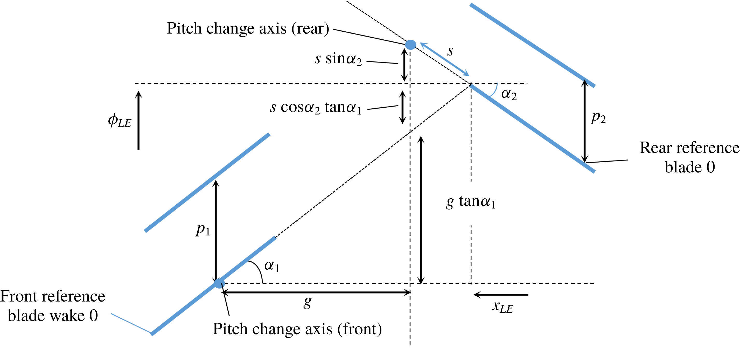
on the leading edge of the downstream blade. By geometric considerations (see figure 2), we find that
 $x_{LE}(z)=x_{PCA_{2}}-M_{x}S(z)$
and
 $\unicode[STIX]{x1D719}_{LE}(z)=\unicode[STIX]{x1D719}_{PCA_{2}}-M_{t_{2}}S(z)$
, where
 $x_{PCA}$
and
 $\unicode[STIX]{x1D719}_{PCA}$
are the axial and azimuthal locations of the pitch change axes,
 $\unicode[STIX]{x1D6FC}_{2}$
is the local (rear blade) helicoidal propeller advance angle used by Hanson (Reference Hanson1980, Reference Hanson1985), such that
 $\cos \unicode[STIX]{x1D6FC}_{2}=M_{x}/M_{r_{2}}$
and
 $\sin \unicode[STIX]{x1D6FC}_{2}=zM_{t_{2}}/M_{r_{2}}$
, and, for convenience, we have introduced
 $S(z)=s(z)/M_{r_{2}}(z)$
. The location of the leading edge is thus
 $$\begin{eqnarray}\frac{\text{d}x_{LE}}{\text{d}z}=-M_{x}\frac{\text{d}S}{\text{d}z},\quad \frac{\text{d}\unicode[STIX]{x1D719}_{LE}}{\text{d}z}=-M_{t_{2}}\frac{\text{d}S}{\text{d}z}.\end{eqnarray}$$
Two-dimensional interaction geometry.

We now introduce the coordinates of the wake centreline of the front row’s reference blade as
 $[x_{W}(z),z,\unicode[STIX]{x1D719}_{W}(z)]$
so that, when
 $x_{W}=x_{LE}$
, the wake’s centreline location is
 $\unicode[STIX]{x1D719}_{W}(z)=\unicode[STIX]{x1D719}_{PCA_{1}}+M_{t_{1}}S(z)$
, where the wake coordinates are, naturally, measured from the front row’s pitch change axis. Since the relative rotation speed of the two blade rows is
 $M_{t_{1}}+M_{t_{2}}$
and the azimuthal gap between the rear row leading edge and the wake is
 $\unicode[STIX]{x1D719}_{LE}(z)-\unicode[STIX]{x1D719}_{W}(z)$
, we can obtain the times of the leading-edge interactions as
 $\unicode[STIX]{x1D70F}(z)=S(z)$
, where we have arranged
 $\unicode[STIX]{x1D70F}(z)=0$
at the hub where
 $S(z)=0$
. The space-time phase is thus
 $$\begin{eqnarray}\unicode[STIX]{x1D6EC}_{n_{1},n_{2}}(z,\unicode[STIX]{x1D719}_{2},t)=\unicode[STIX]{x1D714}[t-S(z)]-\unicode[STIX]{x1D708}[\unicode[STIX]{x1D719}_{2}-\unicode[STIX]{x1D719}_{LE}(z)],\end{eqnarray}$$
which is zero when
 $\unicode[STIX]{x1D719}_{2}=\unicode[STIX]{x1D719}_{ev}(z,t)$
and an interaction event occurs. Thus, after a little manipulation, we obtain the event line as
 $$\begin{eqnarray}\unicode[STIX]{x1D719}_{ev}(z,t)=\unicode[STIX]{x1D719}_{PCA_{2}}+(\unicode[STIX]{x1D714}/\unicode[STIX]{x1D708})t-(\unicode[STIX]{x1D702}/\unicode[STIX]{x1D708})S(z),\end{eqnarray}$$
which can be differentiated to get
 $$\begin{eqnarray}\frac{\text{d}\unicode[STIX]{x1D719}_{ev}}{\text{d}z}=-\frac{\unicode[STIX]{x1D702}}{\unicode[STIX]{x1D708}}S^{\prime }=-M_{p}vS^{\prime },\end{eqnarray}$$
where a prime denotes differentiation with respect to
 $z$
.
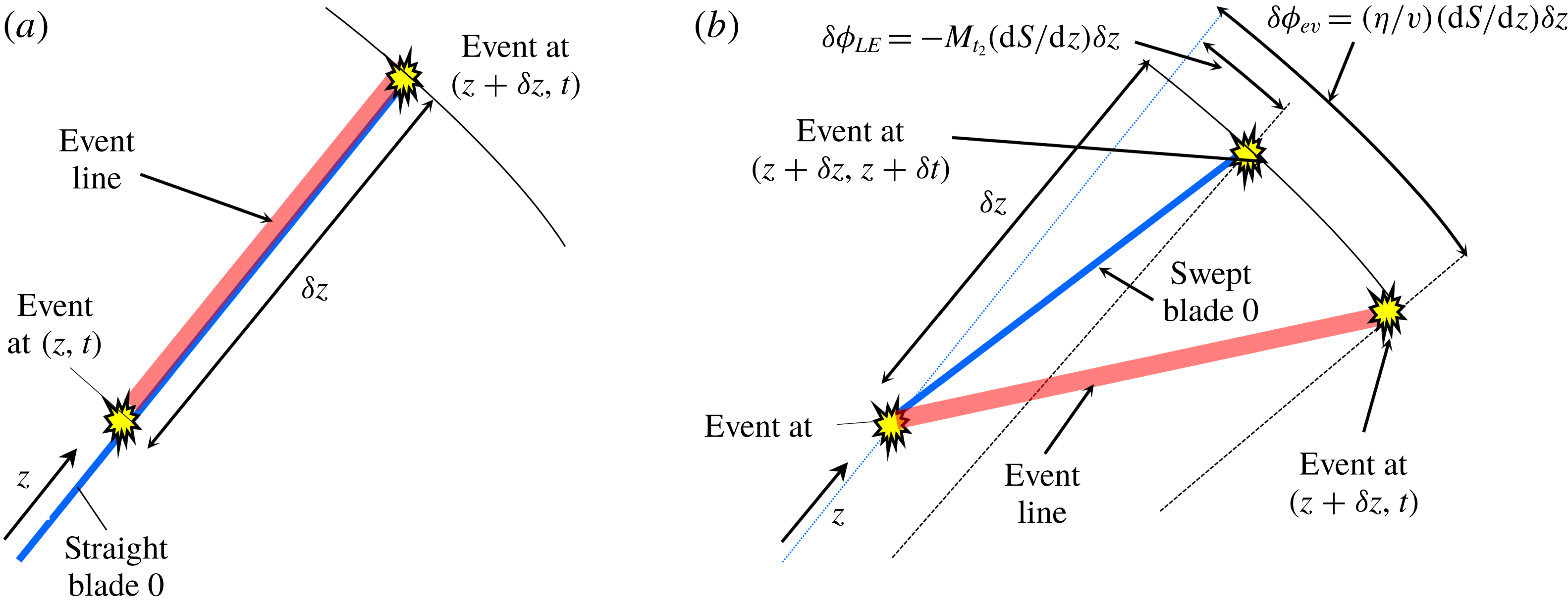
Locations of the rear row blade leading edges and the locus of the interaction events at fixed time: (a) straight blades, (b) swept blades.

The result (3.6) defines the event line as a function of radius
 $z$
and, most importantly, at a fixed time (see figure 3). We recall that this event line represents the locus of points, between the propeller hub and tip, along which the space-time phase
 $\unicode[STIX]{x1D6EC}_{n_{1},n_{2}}$
is zero. These points do not necessarily correspond to the radial distribution of interaction events because the interaction time
 $t$
varies with
 $z$
whereas, for an event line, the time remains fixed. It is also worth noting that the event line is not the same as the downstream propeller’s leading-edge line
 $\unicode[STIX]{x1D719}_{2}=\unicode[STIX]{x1D719}_{LE}(z)$
, even though the space-time phase is zero at the wake interaction points along that line, because, once again, as the wake interaction moves along the downstream blade leading edge, the time is not constant but varies as
 $\unicode[STIX]{x1D70F}(z)$
.
4 Interactions as viewed by the observer
We now consider the location of the interactions from the viewpoint of a fixed observer. The interaction events are all located on the surface of revolution described by the leading edges of the rear row blades, which all move in the positive
 $x$
direction at Mach number
 $M_{x}$
. With
 $\unicode[STIX]{x1D719}_{ev}$
as the azimuthal event location we can obtain the component of the Mach number resolved in the direction of the observer as
 $$\begin{eqnarray}\displaystyle M_{obs}=M_{x}\cos \unicode[STIX]{x1D703}-\mathbb{M},\quad \mathbb{M}=zM_{p}\sin \unicode[STIX]{x1D719}_{ev}\sin \unicode[STIX]{x1D703}, & & \displaystyle\end{eqnarray}$$
where
 $\mathbb{M}$
represents the contribution to
 $M_{obs}$
from the azimuthal speed of the disturbance. Using (2.1) we find that this Mach number is precisely sonic (the sonic condition) when
 $$\begin{eqnarray}\displaystyle \mathbb{M}=-(1-M_{x}\cos \unicode[STIX]{x1D703}),\quad \sin \unicode[STIX]{x1D719}_{ev}=-z^{\ast }/z. & & \displaystyle\end{eqnarray}$$
Now consider the term
 $\mathfrak{l}=(\text{d}x_{ev}/\text{d}z)\cos \unicode[STIX]{x1D703}+(\text{d}y_{ev}/\text{d}z)\sin \unicode[STIX]{x1D703}$
, which represents the dot product of the position vector from the far-field observer to the event at location
 $z$
with a local vector that represents the tangent to the event curve, as a function of
 $z$
, at fixed source time. Since
 $x_{ev}=x_{LE}$
and
 $y_{ev}=z\cos \unicode[STIX]{x1D719}_{ev}$
we can use (3.3) and (3.6) to get
 $$\begin{eqnarray}\frac{\text{d}x_{ev}}{\text{d}z}=-M_{x}S^{\prime },\quad \frac{\text{d}y_{ev}}{\text{d}z}=\cos \unicode[STIX]{x1D719}_{ev}+z\sin \unicode[STIX]{x1D719}_{ev}M_{p}S^{\prime },\end{eqnarray}$$
so that, using (4.1b
) and (4.2a
),
 $\mathfrak{l}=-S^{\prime }+\sin \unicode[STIX]{x1D703}\cos \unicode[STIX]{x1D719}_{ev}$
and thus
 $\mathfrak{l}=0$
, and the line from the observer to an interaction location at radial station
 $z$
is normal to the local tangent of the event curve (the normal-edge condition), when
 $$\begin{eqnarray}\sin \unicode[STIX]{x1D703}\cos \unicode[STIX]{x1D719}_{ev}=S^{\prime }.\end{eqnarray}$$
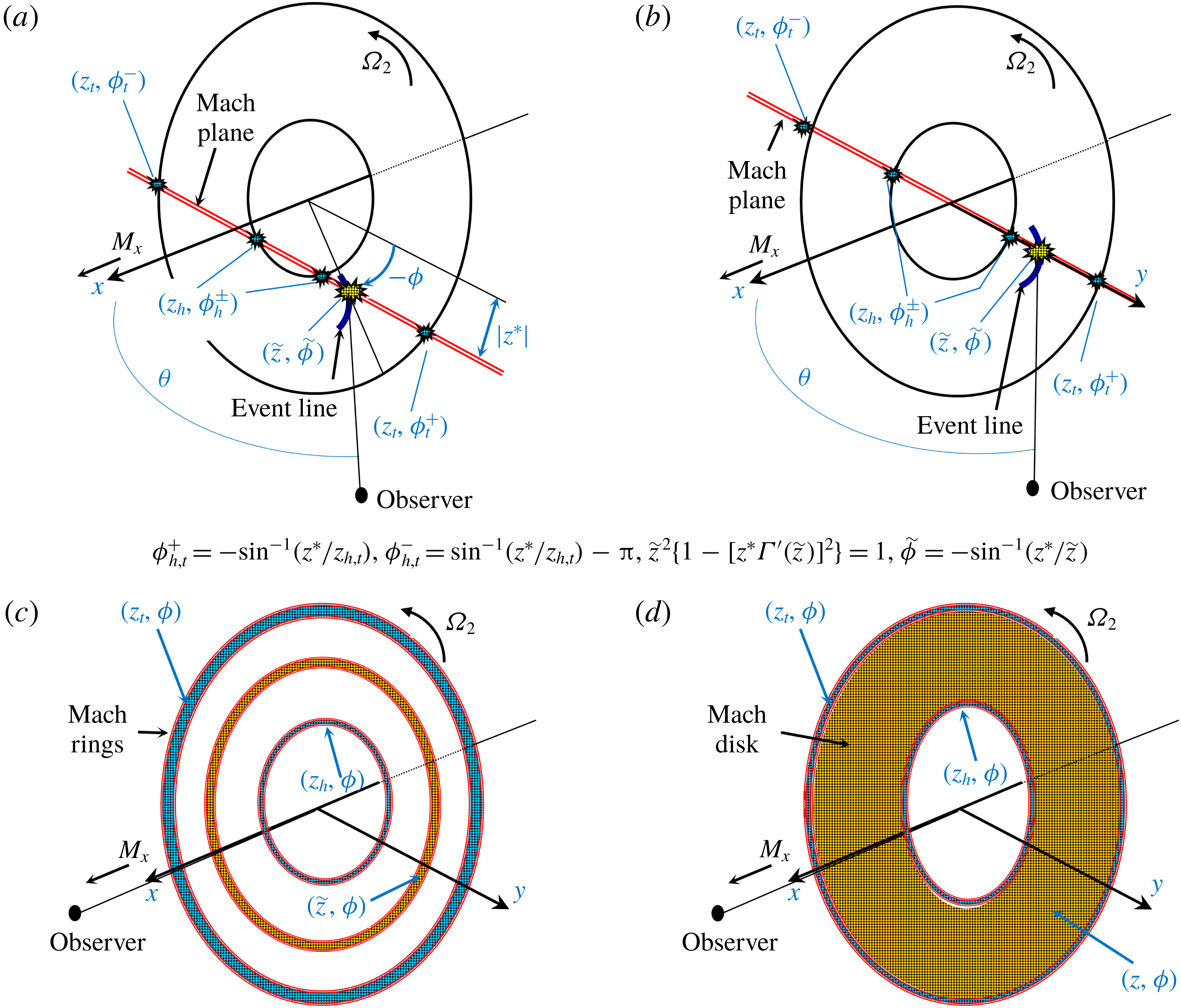
Mach plane and interaction events (a)
 $\unicode[STIX]{x1D708}\rightarrow \infty$
,
 $\unicode[STIX]{x1D703}\neq 0$
, swept; (b)
 $\unicode[STIX]{x1D708}=0$
,
 $\unicode[STIX]{x1D702}\rightarrow \infty$
,
 $\unicode[STIX]{x1D703}\neq 0$
,
 $z^{\ast }=0$
, swept; (c)
 $\unicode[STIX]{x1D708}=0$
,
 $\unicode[STIX]{x1D702}\rightarrow \infty$
,
 $\unicode[STIX]{x1D703}=0$
,
 $z^{\ast }=0$
, swept; (d)
 $\unicode[STIX]{x1D708}=0$
,
 $\unicode[STIX]{x1D702}\rightarrow \infty$
,
 $\unicode[STIX]{x1D703}=0$
,
 $z^{\ast }=0$
, straight.

From the definition of sweep in (2.2) we see that (4.4) is equivalent to
 $\cos \unicode[STIX]{x1D719}_{ev}=z^{\ast }\unicode[STIX]{x1D6E4}^{\prime }(z)$
, so that, combining it with (4.2b
), we obtain Kingan & Parry’s (Reference Kingan and Parry2019) requirement (2.3) for interior stationary points in the radiation integral. We have thus shown that the locations that dominate contra-rotating propeller sound radiation of an
 $(n_{1},n_{2})$
combination tone to the far field represent the points on the rear row leading edge that satisfy the sonic condition and the normal-edge condition. These criteria were discovered by Amiet (Reference Amiet1988) and Parry (Reference Parry1995) for a single-rotating propeller, in the time and frequency domains, respectively, but there the event curve was merely the blade leading edge itself. Here, clearly, the difficulty lies in determining both the shape and speed of the event curve, as neither the shape nor the speed coincides with that of either the front or rear blades. For clarity, the locations of the Mach plane and the source satisfying the normal-edge and sonic conditions are illustrated in figure 4(a) for a typical swept blade case.
Points on the boundary are, by definition, located at the hub and tip, whatever the shape of the blade leading edge there, so it follows that they do not automatically satisfy the normal-edge condition. However, from (4.2) it is clear that points at the hub and tip satisfy the sonic condition when
 $\sin \unicode[STIX]{x1D719}_{ev}=-z^{\ast }/z_{b}$
, where
 $z_{b}$
is the hub or tip radius (
 $z_{h}$
or
 $z_{t}$
). The two solutions are precisely the same as those given by (2.4) with the dummy variable
 $u$
replaced by
 $-\unicode[STIX]{x1D719}$
.
The boundary points are shown in figure 4(a) with the two tip boundary points and the two hub boundary points also lying on the Mach plane. The tip boundary points exist if
 $z^{\ast }<z_{t}$
and the hub boundary points exist if
 $z^{\ast }<z_{h}$
.
5 Zero-order modes
When the azimuthal mode number
 $\unicode[STIX]{x1D708}$
becomes small, or zero, Kingan & Parry (Reference Kingan and Parry2019) found that the interior stationary points were defined by
 $$\begin{eqnarray}\displaystyle \unicode[STIX]{x1D6E4}^{\dagger ^{\prime }}(z)=\pm 1/z^{\dagger },\quad u=0\text{ or }\unicode[STIX]{x03C0}, & & \displaystyle\end{eqnarray}$$
where
 $u$
is the azimuthal angle and the revised sweep phase factor and non-dimensional radius terms are
 $$\begin{eqnarray}\displaystyle \unicode[STIX]{x1D6E4}^{\dagger }(z)=\frac{1}{z^{\dagger }\sin \unicode[STIX]{x1D703}}S(z)+\unicode[STIX]{x1D706}^{\dagger }g\frac{M_{t_{1}}}{M_{x}}\quad \text{and}\quad z^{\dagger }=\frac{(1-M_{x}\cos \unicode[STIX]{x1D703})}{\sin \unicode[STIX]{x1D703}}, & & \displaystyle\end{eqnarray}$$
respectively, where
 $\unicode[STIX]{x1D706}^{\dagger }=n_{2}B_{2}/\unicode[STIX]{x1D702}=1/(M_{t_{1}}+M_{t_{2}})$
, and
 $\unicode[STIX]{x1D702}$
is the formally large parameter.
We can follow the analysis of § 4 to show that the sonic condition is satisfied when
 $$\begin{eqnarray}\displaystyle \sin \unicode[STIX]{x1D719}_{ev}=-\frac{1}{M_{p}}\frac{z^{\dagger }}{z},\quad \frac{\text{d}\unicode[STIX]{x1D719}_{ev}}{\text{d}z}=-M_{p}S^{\prime }, & & \displaystyle\end{eqnarray}$$
and, as before, the normal-edge condition is satisfied if (4.4) is satisfied. The combination of (4.4), (5.2) and (5.3), along with
 $\unicode[STIX]{x1D708}=0$
, ensures that we recover (5.1) with
 $\unicode[STIX]{x1D719}_{ev}=0$
or
 $\unicode[STIX]{x03C0}$
. The result is particularly interesting as it shows that points exist that satisfy the normal-edge and sonic conditions, even though the angular speed
 $M_{p}$
of the disturbance is infinite. For
 $\unicode[STIX]{x1D708}=0$
these solution points lie on a plane containing the observer and the propeller axis (
 $\unicode[STIX]{x1D719}_{ev}=0$
or
 $\unicode[STIX]{x03C0}$
) – as they must because, at any other azimuthal location, the component of the event speed, resolved in the direction of the observer, is infinite. As the angular speed of the harmonic disturbance and
 $\text{d}\unicode[STIX]{x1D719}_{ev}/\text{d}z$
are infinite, the event line corresponds to a local arc of a ring which is, consequently, normal to the radial direction at any
 $(z,\unicode[STIX]{x1D719})$
location. An illustration is shown in figure 4(b) for a typical swept blade case in which the Mach plane is coincident with the
 $(x,y)$
plane where the source is located and for which the normal-edge and sonic conditions are satisfied; the event line and the hub and tip boundary points are also indicated.
For
 $\unicode[STIX]{x1D708}=0$
and
 $\unicode[STIX]{x1D703}=0$
Kingan & Parry (Reference Kingan and Parry2019) found, through the simplification of the phase argument in the radiation integral, that the asymptotic result for sound radiation reduced to a single integral over
 $z$
, and concluded that it represented a continuum ring of stationary points in the general case and a continuum annular disk in the straight-bladed case. Their results can be explained in physical terms because, for
 $\unicode[STIX]{x1D703}=0$
, the sonic and normal-edge conditions are satisfied at all azimuthal locations, as the analysis of § 4 reduces to the simple result
 $S^{\prime }=0$
or, from (5.2),
 $\unicode[STIX]{x1D6E4}^{\dagger ^{\prime }}(z)=0$
, which specify the radius at which the ring is located; the event line is coincident with the ring. Of course,
 $\unicode[STIX]{x1D6E4}^{\dagger ^{\prime }}(z)=0$
is satisfied at all radii for a straight-bladed propeller and the entire annulus satisfies the sonic and normal-edge criteria; the event line in this case becomes an event disk, as the interaction events happen simultaneously at all locations. Illustrations are shown in figure 4(c,d).
6 Conclusions
We have interrogated the work of Kingan & Parry (Reference Kingan and Parry2019) to explain the physical meaning underlying the critical sources of propeller wake interaction noise. The critical points lie on an event line – where, at each radius, we have followed Tyler & Sofrin’s (Reference Tyler and Sofrin1962) definition of an event – and satisfy the normal-edge and sonic conditions. These two conditions were discovered by Amiet (Reference Amiet1988) in the time domain and Parry (Reference Parry1995) in the frequency domain for a single-rotating propeller, but in their analyses the relevant radial line was merely the blade leading edge itself. Here, for wake interaction noise, the difficulty lies in determining the event curves shape and speed, as neither coincides with that of either the front or rear blades. The event line rotates around the annulus at the speed of the interaction mode and represents the locus of the interactions between the rear blade leading edge and the upstream wake, where it is essential to note that this locus must be determined at a fixed point in time; the mode rotation speed, and the times at which the interactions occur, can thus be used to calculate the event line from the real space-time locus of the interactions. The points satisfying the normal-edge and sonic conditions (critical sources) lie on the Mach plane a distance
 $z^{\ast }$
from the
 $(x,y)$
plane.
Kingan & Parry (Reference Kingan and Parry2019) also obtained asymptotic solutions for the radiation when
 $\unicode[STIX]{x1D708}=0$
and the mode rotation speed is infinite. However, we have shown here that, surprisingly, the sonic and normal-edge conditions can still be satisfied at certain locations in the
 $(x,y)$
plane and that, in this case, the event line becomes an arc of a ring. For radiation directly along the axis, with
 $\unicode[STIX]{x1D703}=0$
, we have shown that the sonic and normal-edge conditions can be satisfied at all azimuthal locations, and the dominant sources for a swept- or straight-bladed propeller thus form a continuum ring or annulus, respectively, and the event line becomes a ring or disk, respectively.
We have shown too that the lower-order boundary points at the tip and hub also satisfy the sonic condition (but not the normal-edge condition) and these points also lie on the Mach plane (or Mach ring), precisely as for the dominant sources.
In § 1 we pointed out that lean (both aerodynamic and geometric) has been neglected in the analysis. Such lean effects change the locations of the convected distortion–blade interaction and will, therefore, change the location of the event line relative to that on a propeller design that has sweep but no lean. Nonetheless, even with lean, the role of the event line – in representing the locus of the interaction locations at a fixed point in time – remains the same as that described here.