1. Introduction

The ice flow at an ice-stream margin is three-dimensional (3-D). Typically, a strong lateral gradient in downstream velocity causes intense shearing between the stream and interstream areas, while ice crosses the margin into the stream. Margins as narrow as a few kilometres are common, potentially due to shear localization by strain heating and the development of ice anisotropy (see review by Reference Raymond, Echelmeyer, Whillans, Doake, Alley and BindschadlerRaymond and others, 2001). Shear margins control the ice flux conveyed by an ice-stream tributary or ice-stream trunk because they exert side drag on the flow and their positions govern the flow width (Reference RaymondRaymond, 2000). Margin migration, involving the mobile transition in basal lubrication between stream and interstream areas, influences ice-stream stability (see, e.g., Reference SchoofSchoof, 2004; Reference Sayag and TzipermanSayag and Tziperman, 2009).

Remote-sensing images captured by the 5.3 GHz synthetic aperture radar (SAR) of the RADARSAT Antarctic Mapping Project (Reference JezekJezek, 1999; Reference JezekJezek and others, 2002) reveal many unexplained features on the ice-sheet surface, and some of these features occur at ice-stream margins. On RADARSAT images, the digital number (DN) representing radar backscatter intensity or ‘brightness’ at each position measures subsurface as well as surface properties (e.g. slope and roughness) because radar waves at 5.3 GHz can penetrate polar firn to depths of the order of 10m (Reference Bingham and DrinkwaterBingham and Drinkwater, 2000; Reference Rignot, Echelmeyer and KrabillRignot and others, 2001). Ice-stream margins appear on these images as curvilinear features that look bright where surface crevasses are abundant (an example occurs near the right border of Fig. 1a), and elsewhere as curvilinear, near-parallel bands of contrasting brightness that extend for many kilometres or that are less continuous. Figure 1a shows an example of an ice-stream marginal feature from a tributary of Bindschadler Ice Stream, West Antarctica, consisting of multiple discontinuous bands. In this paper, we derive insights into how such features form by studying this example.

Fig. 1.

(a) RADARSAT Antarctic Mapping Mission-2 (AMM-2) mosaic and (b) MODIS mosaic of the onset zone of Bindschadler Ice Stream, at 25 m and 125 m pixel resolutions, respectively. The inset in (a) locates the study area. The ice stream flows from top left to bottom right. The curvilinear and multiple-banded RADARSAT backscatter feature on the southern margin of the ice stream, located in the area between dashed curves in (a) and crossed by radar lines M, K and H, is investigated in this paper. Contours in (b), at 10 m a^–1 intervals, represent surface flow speed from Reference Rignot, Mouginot and ScheuchlRignot and others (2011). In both panels, CMP marks the common-midpoint survey that determined the wave speed in firn for converting the two-way travel time of radar traces to depth in the radargrams in Figure 2.

Because the ice-stream marginal features can resemble ‘flow stripes’ on ice streams (Reference Glasser and GudmundssonGlasser and Gudmundsson, 2012) and often occur near them, they have been included in studies that map flow stripes to understand ice-flow history (e.g. Reference Hulbe and FahnestockHulbe and Fahnestock, 2007); some marginal features have enabled inferences of ice-stream reorganization (Reference Jacobel, Scambos, Nereson and RaymondJacobel and others, 2000; Reference Conway, Catania, Raymond, Gades, Scambos and EngelhardtConway and others, 2002). However, the marginal features and flow stripes may have different causes. Flow stripes can form as a result of fast ice flow over bed areas with uneven topography or slipperiness and the dynamical transmission of such variability to the surface (Reference Gudmundsson, Raymond and BindschadlerGudmundsson and others, 1998). In contrast, here we explore a near-surface explanation for the marginal features, even though the basally driven mechanism may also create them. The term ‘flow stripe’ has been used in the literature to refer to features identified by either their topographic or RADARSAT-brightness expression (see, e.g., Reference Gudmundsson, Raymond and BindschadlerGudmundsson and others, 1998; Reference Conway, Catania, Raymond, Gades, Scambos and EngelhardtConway and others, 2002). When analysing the multi-banded ice-stream marginal feature in Figure 1a, we distinguish between these attributes, as they are different.

We first report our observations of this marginal feature in Section 2, linking together (1) its brightness expression on the RADARSAT image, (2) stratigraphic undulations in the firn evidenced by radargrams crossing the feature and (3) the surface topography along these radar transects. This approach establishes a strong correlation between the RADARSAT digital number (DN) and radar-layer depth, as has been found by Reference Gray, Conway, King and SmithGray and others (2008), who used the same approach to study flow stripes on Kamb Ice Stream, West Antarctica. We follow some earlier studies in assuming that radar layers are isochrones, despite a potentially complex pattern of strain rates at our ice-stream margin. The correlation thus prompts us to view the RADARSAT brightness expression as indicating 3-D wavy isochronal surfaces within the firn. This motivates our mathematical model in Section 3, which describes isochrone depth evolution under the near-surface flow field of an ice-stream margin. Although the model is exploratory and simplistic (e.g. ice flow is prescribed rather than found by solving the Stokes equations; feedback by surface topography on accumulation rates is ignored), the shape of isochrones simulated by it shows that banded RADARSAT expressions will form under the expected flow at shear margins. Notably, if there are fluctuations in flow acceleration along the ice stream, then the shear-margin bands must ‘break up’ in a similar manner to that shown by our observed feature.

2. Observations

Figure 1 shows the RADARSAT image and the Moderate Resolution Imaging Spectroradiometer (MODIS) image (Reference Haran, Bohlander, Scambos and FahnestockHaran and others, 2005) of our study site in the onset zone of Bindschadler Ice Stream. In this region, surface flow speed increases from 50 m a^-1 to 100 m a^-1 along the ice-stream centre line, and recent modelling of radar-detected firn stratigraphy along the centre line suggests that the ice flow has been roughly steady for the past ∼400 years (Reference Ng and KingNg and King, 2011).

The multi-banded feature occurs on the southern ice-stream margin (similar features on the northern margin are not examined in this paper). Its RADARSAT expression consists of three prominent bands that track the margin for a distance of ∼40km (Fig. 1a). Analysis of surface velocities derived from interferometric SAR (InSAR) measurements by Reference Rignot, Mouginot and ScheuchlRignot and others (2011) shows that flow speeds jump by tens of metres per year across the margin, which is several kilometres wide (see the contours in Fig. 1b), and that the velocity component of ice crossing the margin into the ice stream is ∼10ma^–1. Although the bands in Figure 1a look sinuous, inspection of their alignment shows that each band may be a straighter feature, the brightness of which fades and recovers along its length. In this interpretation, the dark-bright-dark sequence of the three parallel bands upstream of line M switches into a bright-dark-bright sequence downstream of this line. Another switch is seen midway between lines K and H, and a more subtle switch occurs across line K. These brightness reversals occur every 10 km or so.

The MODIS image in Figure 1b primarily reflects variations in ice-surface slope, highlighted by an effective illumination from the south. While its grey-shaded pattern is not identical to that of the RADARSAT image in Figure 1a, we recognize similarities between the two images: for instance, some MODIS features are aligned with the marginal bands on the RADARSAT image. This suggests that the RADARSAT expression carries some information about surface topography.

Figure 2 presents radargrams of the firn along three lines M, K and H (white lines in Fig. 1) crossing our marginal feature, measured as part of a ground-based 100 MHz radar survey network in the 2001/02 austral summer. In building these radargrams, the two-way travel time of radar traces has been converted to depth by using the electromagnetic wave speed in firn measured by a common-midpoint survey at the site labelled CMP in Figure 1; further radar processing details are given by Reference Woodward and KingWoodward and King (2009) and Reference Ng and KingNg and King (2011). All three radargrams display major undulations or ‘folds’ in the internal layers where they intersect the RADARSAT expression at the margin (at y≈8-11 km on line M, 6-9 km on line K and 5-8 km on line H). Down to at least 20 m depth, these folds tend to increase in amplitude with depth; deeper down, their geometry becomes less clear owing to stronger attenuation of radar waves in a zone coinciding with the ice-stream margin. Moving downstream from lines M to K to H, the dominant layer folds change shape from ‘W’ to ‘N’ to ‘M’, accompanied by variations in the tilt of hinge lines linking their crests and troughs. These changes make it difficult for us to connect the folds across the radargrams, as Reference Ng and ConwayNg and Conway (2004) have done for deep radar layers in Kamb Ice Stream. Also, on line H, an ‘eye feature’ (see Reference Arcone, Spikes and HamiltonArcone and others, 2005) occurs at y=5.5 km and 30 m depth that is absent on the other two radargrams.

Fig. 2.

Observed properties along lines (a) M, (b) K and (c) H in Figure 1, including elevation sand slope ∂s/∂y of the ice surface, smoothed profile of the RADARSAT backscatter intensity or brightness value DN, firn stratigraphy detected by our ground-based radar profiling, and the shape of a prominent radar layer ∼10-15 m deep picked from each radargram. The two ends of this layer are marked by triangular symbols on each radargram. In all three panels, the ice-stream flow is towards the observer. Boxes labelled ‘W, ‘ᴻ’ and ‘M’ highlight the dominant layer folds described in the text. Labels under the radargrams show the approximate width of the ice-stream shear margin, identified from where flow-speed contours in Figure 1b are close together. In (a) we include an extra (lowermost) radargram that has been corrected for surface topography, to show the elevation change along the radar layers.

A key question is how the layer folds relate to the planimetric expression of the marginal feature. Above each radargram in Figure 2 we plot surface elevation s, surface slope ∂s/∂y, and RADARSAT backscatter intensity (represented by digital number, DN) along each transect. DN in this figure is the spatial average of DN values over an area that measures ∼1km × ∼350m about each point and that has long axis perpendicular to the y-direction. All three lines show correlation between the layer undulations and variations in DN, especially for layers at ∼-10-20m depth, which is similar to the expected depth of penetration of the SAR waves into firn (Reference Bingham and DrinkwaterBingham and Drinkwater, 2000; Reference Rignot, Echelmeyer and KrabillRignot and others, 2001). Correlation between DN and layer depth is observed outside the ice-stream margin as well as in the regions of the dominant layer folds, and the DN curves reproduce the shape sequence W to N to M of the folds. In Figure 2, we highlight this correlation by picking a prominent radar layer ∼-10-15m deep on each radargram and plotting its depth profile. Although the correlation has some uncertainty (e.g. it is shifted by a fraction of a kilometre on lines M and K), it seems convincing to us and difficult to ignore. If we assume that it holds across our study area, then bright areas on the RADARSAT image correspond to layer crests in the firn, and dark areas to layer troughs.

As mentioned before, a similar result was found by Reference Gray, Conway, King and SmithGray and others (2008) on Kamb Ice Stream. Those authors invoked volumetric backscatter of the SAR waves in the firn to explain why DN covaries with the near-surface stratigraphy. They suggested that, since the number of hoar/frost horizons in the firn above a given isochronal layer should be similar over a region of the ice sheet, their density would be high where the layer is shallow, enhancing the RADARSAT backscatter (and the converse). If this is true, then we can regard the RADARSAT expression in Figure 1a as portraying the depth variation of shallow, 3-D isochronal layers in plan view. In this interpretation, the inferred layer geometry at our ice-stream margin exhibits multiple folds with axes aligned roughly along it, and the brightness reversals seen on the RADARSAT bands reflect the changing configuration of fold axes and development of new layer structures along the margin.

But what causes folding of the shear-margin stratigraphy? Assuming the layers to be isochronal, their shape may register the cumulative effects of (1) horizontal strain rates that thin or thicken the firn, (2) ice-flow advection, (3) spatial variation in accumulation rate and (4) firn densification (Reference Ng and KingNg and King, 2011). We formulate a model for this in Section 3. Ice flow at the shear margin is expected to have complicated strain-rate and advection patterns (factors 1 and 2). In addition, it may generate surface topography that induces non-uniform accumulation via atmospheric coupling (factor 3). Figure 2a–c show that the layer undulations correlate not with surface elevation but selectively with surface slope where the folds occur, suggesting that factor (3) operates to some extent; we noted earlier that the RADARSAT image carries a surface-slope signature. For reasons given below, however, we exclude this factor from our modelling.

3. Mathematical Model

We study the hypothesis that ice flow at shear margins creates isochronal-layer geometry that explains the key characteristics of the RADARSAT expression: both its banding and brightness reversals. In the current analysis, we restrict our aim to demonstrating this possibility, rather than building a comprehensive model of the observations. Our model is kinematic. It tracks how isochrones evolve under prescribed flow fields; we do not solve for the ice flow through mechanical considerations (cf. Reference Jacobson and RaymondJacobson and Raymond, 1998; Reference SchoofSchoof, 2004).

3.1. Isochrone depth evolution

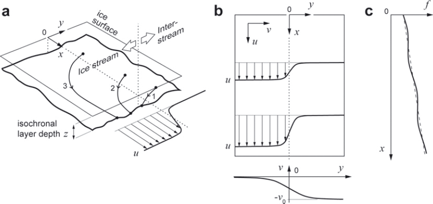
Figure 3a illustrates our system. We denote the depth of an isochrone by z(x, y, t), where t is time, x is the downstream coordinate, and y is the cross-stream coordinate (pointing towards the interstream), with y=0 located in the marginal zone. As z is defined with respect to the surface, layer-depth variations in this model may be compared directly with those on the radargrams in Figure 2 (which use z as vertical coordinate) whether or not the surface topography undulates. We prescribe a steady horizontal velocity field u = (u, v) throughout the depth of the firn (the top ∼100m of the ice sheet), where u and v, the downstream and cross-stream velocity components, are functions of x and y (Fig. 3b). Thus the firn is passively advected by the underlying ice flow, the 3-D motion of which is not treated. As each firn column moves, it stretches or compresses under gradients of u and v, receives surface accumulation at a rate a, and compacts vertically (densification). According to Reference Ng and KingNg and King (2011), an evolution equation for isochrone depth that encapsulates these processes is

(1)

Fig. 3.

Schematic and symbols of our mathematical model of isochrone depth evolution at an ice-stream margin. (a) Three-dimensional geometry of an isochronal layer, z(x, y, t), where z is layer depth, t is time, x and y are downstream and cross-stream coordinates, respectively, and y=0 is the centre of the shear margin. Curves 1, 2 and 3 indicate historical trajectories of material particles lying on the same isochronal layer, assuming the velocity field in (b). (b) Prescribed fields of downstream velocity u and cross-stream velocity v across the margin. The upper box shows u(x, y) defined by Eqns (4-6). The lower graph shows the cross-stream dependence of v defined by Eqn (7) with y0=0. (c) Two forms of the function f(x) used to impose longitudinal variations on the downstream velocity u. The dashed line is linear (α>0 and 6=0 in Eqn (5)). The solid line is linear plus sinuisoidal (α>0 and <δ>0 in Eqn (5)).

where ∇. is the horizontal divergence operator (e.g. ∇.u = ∂u/∂x + ∂v/∂y), ρ(z) is the density-depth profile of the firn (assumed invariant with x and y) and p₀ is the firn surface density. Eqn (1) derives from mass conservation and is equivalent to some models that correct the submergence rate of material particles for densification when tracking layers (see, e.g., Reference Arcone, Spikes and HamiltonArcone and others, 2005; Reference Woodward and KingWoodward and King, 2009). Under steady ice flow, forward simulation of Eqn (1) generates a stationary pattern of isochrones, and t refers to their age (see Reference Ng and KingNg and King, 2011).

Equation (1) has the provision of including feedback on the accumulation rate induced by surface topography that develops at the shear margin (see discussion at the end of Section 2) because a = a(x, y, t) may be linked to processes such as katabatic wind flow and snow redistribution. However, modelling this feedback requires treatment of atmospheric coupling and shear-margin thermomechanics down to the ice-stream bed, neither of which is straightforward, especially in 3-D. In this paper, we assume a to be constant in order to avoid tackling these processes. This assumption does not invalidate our aim set out above.

By using the change of variable

(2)

Eqn (1) can be simplified to

(3)

where the ‘transformed’ isochrone depth, Z(x, y, t) accounts for densification. In our simulations, we solve Eqn (3) for Z and recast isochrones in true depth before plotting them. We assume the firn density-depth profile ρ(z) = ρ _i – (ρ _i – ρ₀)e^–cz with pi = 917 kg m–³, ρ₀ = 400kgm^–3, and c=1/35m–¹ measured in ITASE core 99-1 (Reference Arcone, Spikes and HamiltonArcone and others, 2005), which is the nearest firn core to our site, located 37.5 km upstream of line M.

3.2. Velocity field

In a typical ice-stream margin, we expect u to be small in the interstream (y ≫ 0) but to attain large values in the ice stream (y << 0), and expect v to be negative (directed towards the ice stream) and to decay as we cross the margin in the -y-direction; see Figure 3b. This flow field approximates the situation in Figure 1, where the ice stream also accelerates along flow.

To mimic the shapes of these transitions, we prescribe a separable form for the downstream velocity

(4)

in which u₀ is a reference flow speed far out in the ice stream, and the functions

(5)

and

(6)

describe longitudinal and lateral variations of u (Fig. 3b and c). In Eqn (6), β scales the shear-margin width, and g(y) has the limits 0 and 1 as y tends to +∞ and -∞, respectively; its form resembles, for instance, the measured velocity profile in figure 4 of Reference Raymond, Echelmeyer, Whillans, Doake, Alley and BindschadlerRaymond and others (2001). In Eqn (5), a sets the background rate of ice-stream acceleration, and the sine term (with amplitude and wavelength λ) simulates spatial variations in this, as may be caused by uneven ice-stream basal topography or slipperiness. Figure 3c sketches the form of the function f (x).

For the cross-stream velocity we prescribe

(7)

where v ₀ is the flow speed on the interstream far from the margin (Fig. 3b, lower graph), 7 sets the width scale of the decay, and y₀ is a lateral offset used in our later experiments.

These prescriptions are not the only possible choices, but suffice to demonstrate a variety of isochrone geometries that could form at the margin.

3.3. Preliminary analysis

We can anticipate some aspects of isochrone evolution in this model. By expanding Eqn (3) as

(8)

we see that the forcings behind this evolution are: (1) the constant accumulation rate (the first term on the right), which depresses layers uniformly as they age, (2) advection of layers by the velocity field (u, v) (the first bracketed term on the right), and (3) the net vertical compressive strain rate (terms in the last bracket on the right), which elevates layers towards the surface.

Far out in the ice stream, v vanishes so the net strain rate is ∂u/∂x= u0[α + (2πδ/X) cos (2πδx/λ)], solely due to the ice-stream acceleration. If no layer structures are advected from upstream, then the layers there would submerge at a slower rate than a that is uniform if S = 0. Far in the interstream ∂u/∂x and ∂v/∂y vanish; but as we enter the marginal zone, ∂u/∂x (>0) and ∂v/∂y (<0) grow to cause a net strain-rate pattern that depends on the model parameters. Not just this factor, but also its interplay with advection, determines the depth of isochrones here. Complex material trajectories are also expected. Figure 3a depicts trajectories arriving at three points on an isochrone transect spanning the margin. Despite being of the same age, the material particles have been advected by different velocities and travelled vastly different distances.

3.4. Numerical simulations

Four experiments were performed with the model, including one where the simulated isochrones would cause a RADARSAT expression similar to the one in Figure 1a. We solved Eqn (3) with the finite-difference method on a 50 km x 15 km domain (0 < x< 50, -7.5 < y< +7.5), evolving an isochrone initially at z=0 forward in time, to simulate 3-D layers of different ages. We assumed a periodic domain in the x-direction, and precluded layer structures from entering it from the sides by setting the boundary condition ∂Z/∂y = 0 there, so that all simulated structures must be due to the imposed forcings. We used the accumulation rate a = 0.25 m a^-1 (0.1 m w.e.a^-1) and u ₀ = 50 ma–¹ and a = 0.02 km^-1 for the downstream velocity u (consistent with the ice-stream acceleration on our site), with β=0.5km. For the lateral velocity v, we assumed v ₀ = 5 m a^-1, and 7 = 1 km to describe a more gradual transition than in u. Where the sine term in Eqn (5) applies, λ = 20km. In our experiments, we activated this fluctuation on the acceleration by altering 8, and used y₀ in Eqn (7) to offset the lateral and downstream velocity transitions. In reality, these transitions are unlikely to be precisely antisymmetric with inflexion points at the same place.

The first two experiments recreated linear band morphologies. When = y₀ = 0 (constant ice-stream acceleration and no offset), the modelled isochrones express a single set of troughs at the margin, as shown by the results in Figure 4a. This fold forms from the strong lateral compression (∂v/∂y < 0) there. It runs the length of the domain, with an off-vertical hinge line due to ice crossing the margin into the ice stream. Figure 5a plots the depth of the 80-year-old isochrone (thickened isochrone in Fig. 4a, ∼15m deep) over the domain, using light grey where the layer is shallower and dark grey where it is deeper, in the same way as the RADARSAT backscatter imagery would render its depth variation (Section 2). The fold causes a single dark band in plan view. In the second experiment, we shifted the cross-stream velocity field v(y) sideways by setting y ₀=-2km in Eqn (7) and kept other model parameters unchanged. The offset moves the velocity profile at the bottom of Figure 3b (and hence the position of strongest lateral compression) towards the ice stream. Figure 4b shows that the simulated layer troughs are relocated to y = -2km, but we see a new set of layer crests to their right; these form because longitudinal stretching in the ice stream (in y<0, including y 0) elevates all of the layers there above their interstream levels. The resulting feature in plan view is a double band (Fig. 5b). Although our choice here of y ₀ = -2 km is arbitrary (it is not based on measurements but is consistent with the width scale of shear margins), further experiments showed that a negative offset y ₀<0 is necessary to produce a double band in the model.

Fig. 4.

Simulated depth of isochrones across the ice-stream margin at the positions indicated by dashed lines in Figure 5, as produced by different model runs with the parameters (a) =0, y ₀ = 0km, (b) =0, y ₀=-2 km and (c, d) 5 = 0.05, y ₀ = -2 km. (c, d) show layer cross sections from the same model run but at two different downstream positions. In all panels, the ice-stream flow is towards the observer, y=0 is the approximate centre of the shear margin, and the isochrone age interval is 10 years. Thicker curves identify the 80-year-old isochrones for which depth variations are depicted in Figure 5.

Fig. 5.

Depth of an 80-year-old isochrone in the firn represented in greyscale in plan view, as simulated by four model runs with the parameters (a) =0, y₀= 0km, (b) =0, y ₀ = -2km, (c) = 0.05, y ₀ = 0 km, and (d) = 0.05, y₀=-2 km. The greyscale portrays layer-depth variation in a similar way to the RADARSAT backscatter expression. In all panels, y=0 is the approximate centre of the shear margin; the ice stream (flowing in the x-direction) and interstream lie in y<0 and y>0, respectively. Dashed lines locate the cross sections in Figure 4a-d.

In these first experiments, the system and the modelled feature are axially symmetric because there are no longitudinal variations in the forcings (u accelerates but ∂u/∂x is constant); particles at the same position in different transverse cross sections experience the same velocity. In the third and fourth experiments, we put 5 = 0.05 and thus switched on the fluctuations on the ice-stream acceleration to upset this symmetry. When y ₀ = 0 (no offset), the simulated layer pattern is still a trough fold as in Figures 4a and 5a, but its shape ‘wobbles’ downstream (Fig. 5c). Layer depths in the ice stream are also perturbed by spatially varying longitudinal strain rate, as shown by the transverse grey ripples in y<0 in Figure 5c. When 5 = 0.05 and y ₀ = -2 km, the result is a mixture of those in Figure 5b and c. The modelled feature is double-banded, with each band oscillating in brightness in the downstream direction (Fig. 5d), and the crests and troughs of layers in different cross sections differ in amplitudes (Fig. 4c and d). The multiple bands and brightness changes simulated here are the hallmark of our marginal feature on Bindschadler Ice Stream. These findings prompted us to look more carefully at the RADARSAT image in Figure 1a; the patchy features with different shades of grey on the ice-stream side of the margin may have a similar origin to the transverse ripples in Figure 5c and d.

Future investigations could use our model as a basis to explain detailed aspects of the observations (e.g. triple bands; changing fold shapes along the margin; the eye feature in Fig. 2c). This might require the use of precise forcings based on the measured velocity field in our study area, consideration of their time dependence, and an elaborate sub-model of how surface topography evolves and influences the rate of accumulation.

4. Conclusions

In this paper, observations and modelling have yielded new insights into the relationships between the surface flow field at ice-stream margins, the firn stratigraphy at these margins and their RADARSAT expression. Our model is preliminary as it omits surface topography and spatial variability in surface accumulation, but it demonstrates that complex features can form at shear margins under steady flow. Using ground-based radar, Reference Vaughan, Corr, Doake and WaddingtonVaughan and others (1999) showed the existence of layer troughs in the firn at the slow-shearing margin between Carlson Inlet and Fletcher Promontory, with a fold structure resembling what we simulate in Figure 4a; our study extends their work to active ice-stream margins and into 3-D. Probing deeper ice, low-frequency radars have detected layer structures below the firn at a relict margin of Kamb Ice Stream that may be a continuation of such troughs (e.g. see fig. 7 of Reference Raymond, Echelmeyer, Whillans, Doake, Alley and BindschadlerRaymond and others, 2001). Modelling these deep structures and deciphering what they mean for the history of shear margins will require isochrone tracking together with full treatment of the thermomechanics of the margins through the ice column.

A key link in the formation mechanism that we propose for the multi-banded feature at the margin of Bindschadler Ice Stream is the correlation between RADARSAT backscatter intensity and the depth of shallow isochrones. This correlation suggests that at least some other features shown by the RADARSAT imagery may reflect isochrone undulations that encode ice-flow and accumulation histories. It may be productive to study these features systematically on a wider scale, by methods similar to the ones used here, to understand their cause and the information they contain. Candidate features to explore include the RADARSAT expressions of other shear margins and of flow stripes. Regarding the expressions of shear margins, the feature we studied in Figure 1a occurs on a stretch of an ice stream where the flow-speed differential and strain rates are below the threshold for crevasse formation. This example shows that sets of buried crevasses are not the only markers of relict margins, and highlights the possibility of using features like the one in Figure 1a to identify relict margins. Regarding the expressions of flow stripes, it seems that precise calculations have yet to be made to connect their mechanical process of formation and the 3-D geometry of their firn-isochrone undulations.