

Introduction
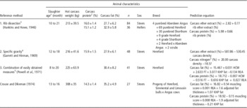
In cattle, carcass composition is an important criterion in the grid of payment to producers. Depending on countries, it has been evaluated through its chemical or its tissue composition. The accurate determination of carcass composition always requires to completely dissect the whole or half carcass. A further step of chemical analysis is required to evaluate the chemical composition of the carcass. This, however, is very costly and cumbersome, and impractical for commercial application. In beef cattle, one way to overcome the difficulty has been to assess carcass composition from partial or indirect measurements (Nour and Thonney, Reference Nour and Thonney1994; Scholz et al., Reference Scholz, Bünger, Kongsro, Baulain and Mitchell2015). To assess the chemical composition of the carcass, three alternative methods have been used: (i) rib dissection (RD) with dissection of the 9th, 10th and 11th rib followed by the analysis of its chemical composition (Hankins and Howe, Reference Hankins and Howe1946), (ii) specific gravity (SG) of the whole carcass (Garrett and Hinman, Reference Garrett and Hinman1969) and (iii) combination of easily obtained measures (EOM) such as the kidney–pelvic–heart fat, USDA yield grade (YG), muscling score, subcutaneous fat thickness (SFT), ribeye area, marbling and hot carcass weight (HCW) (Powell et al., Reference Powell, Huffman and Anthony1971; Crouse and Dikeman, Reference Crouse and Dikeman1974). These methods have become reference methods and form the basis of most of the experiments on the chemical composition of carcass from beef cattle conducted throughout the world. A few publications (e.g. Powell and Huffman, Reference Powell and Huffman1968; Lunt et al., Reference Lunt, Smith, McKeith, Savell, Riewe, Horn and Coleman1985; Miller et al., Reference Miller, Cross, Baker, Byers and Recio1988) evaluated the accuracy of the three methods, and concluded that carcass composition was more accurately determined from RD than from SG and EOM, by decreasing order.
Because the accuracy of measurement differs across reference methods, we hypothesized that this may impact the prediction of carcass composition from proxy traits. A previous study (Al-Jammas et al., Reference Al-Jammas, Agabriel, Vernet and Ortigues-Marty2016) had shown that the proxy traits YG or the SFT in combination with HCW were significantly related to the chemical composition of the carcass determined from the reference methods. In this work, however, data obtained from all reference methods were pooled and no attempt was made to develop relationships for each method.
Hence, current objectives were to evaluate if the relationships between the chemical composition of the carcass and each of the proxy traits (YG, SFT) differed depending on the reference method. The study was conducted by meta-analysis from published results.
Material and methods
International peer-reviewed publications reporting data on the chemical composition of the carcass in cattle were searched using the web of science without restriction on the years. Selection criteria were results of carcass chemical composition from one of the reference methods (Table 1) with at least one proxy trait (YG scaled from 1 to 5 (USDA, 1965), SFT measured in mm in the lumbar region) in cattle. Data extracted from the publications included the detailed description of animals (such as breed, sex and age), the carcass characteristics (HCW, amounts of carcass fat and protein, and proxy data) and the methods of measurement. Animals were further characterized according to the animal typology developed by Al-Jammas et al. (Reference Al-Jammas, Agabriel, Vernet and Ortigues-Marty2016). Sex was defined as: entire male, castrated males, implanted entire males, implanted castrated males. Because of a limited number of data on entire males (implanted or not), and because carcass characteristics of the entire males (implanted or not) and of the implanted castrated males are similar, data from these three categories were grouped together. Breeds were classified according to their production purpose (beef and dual purpose) and their maturing rate (early, intermediate, late maturing breeds).
Summary of the conditions in which each of the three reference methods was elaborated to determine the chemical composition of the carcass in cattle: the animals, the measures and the equations developed to predict carcass fat and protein

1 Slaughter age was not reported in all publications, hence only the range of reported values is indicated here.
2 Carcass protein was as nitrogen×6.25.
3 The rib dissection method consists of dissecting, grinding and chemically analyzing the 9th, 10th and 11th ribs.
4 The specific gravity method consists of weighing the half carcass under water using a triple-beam solution balance suspended over a cylindrical tank (diameter 152 cm; height 168 cm). The carcasses were weighed as rapidly as possible and the water temperature recorded so that carcass density could be corrected to 4°C.
5 The methods referred to as a combination of easily obtained measures are based on the combination of hot carcass weight (HCW, kg), subcutaneous fat thickness (FT, cm), ribeye area (REA, cm2), kidney–heart–pelvic fat (KPH, % of HCW) (Powell et al., Reference Powell, Huffman and Anthony1971) or of muscling score (from 1 to 10 with extremely heavily muscled carcasses scored 1)+REA (cm2)+KPH fat (Crouse and Dikeman, Reference Crouse and Dikeman1974).
Different data sets were constituted, one for each reference method. Publications presenting more than one study were separated into experiments that were individually encoded as such. All data were examined graphically in several steps during the analysis. Descriptive statistics (mean, standard deviation, minimum, maximum) and the normality test for each variable were generated. Methods of meta-analysis were applied intra-study according to Sauvant et al. (Reference Sauvant, Schmidely, Daudin and St-Pierre2008) and Loncke et al. (Reference Loncke, Nozière, Bahloul, Vernet, Lapierre, Sauvant and Ortigues-Marty2015) to take into account the experimental conditions and the influence of other factors of variation. Variance–covariance models were developed on each data set using Minitab software (Minitab® 16.2.4. 2013), as follows:
 $$Y\,{\equals}\,\alpha \,{\plus}\,\alpha _{i} \,{\plus}\,\beta 1\,{\rm HCW}\,{\plus}\,\beta 2\,{\rm X}\,{\plus}\,{\rm error}$$
Where Y is the response variable (carcass fat or protein (kg) measured from one of the reference methods), α the overall (inter-study) intercept, α i the effect of study on α, β1, β2 the coefficients of linear regression of the covariates HCW and X (YG or SFT).
For all models, the normality of residuals was checked (Shapiro and Wilk, Reference Shapiro and Wilk1965) and examined graphically. Outliers were identified based on residuals, high leverage, Cook’s distance and DEFIT as in Sauvant et al. (Reference Sauvant, Schmidely, Daudin and St-Pierre2008). Models were compared by the adjusted R 2, the root square mean error (RMSE), and the coefficients of the models (intercepts and slopes) were compared by t-test.
Results
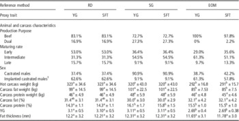
Altogether 25 publications were retrieved, which represented a total of 30 studies and 161 treatments. The RD data set represented 53% of all treatments, the SG 28% and the EOM 19%. All studies were conducted in the United States, but animal characteristics differed across data sets (Table 2). The RD data set included mostly beef breeds (83.1%) with the majority of animals being early maturing (53%), implanted castrated males (62.6%) with the heaviest HCW (323 kg). The SG data set included a slightly smaller proportion of beef breeds (72.7%), with the majority of animals being intermediate maturing (54.5%), castrated males (90.9%), with an intermediate carcass weight (319 kg). Finally, the EOM data set was constituted from beef breeds (>97.8%), intermediate maturing (>51%) and implanted castrated males (>57.8%) with the lightest HCW (291 kg). As a result, carcass fat weight, YG and SFT were significantly lower in the EOM than in the RD and SG data sets. Conversely, the carcass protein weight was similar across data sets. For a given reference method, the meta-design was similar across proxy traits.
Description of animal characteristics in the three data set defined by the reference method used to determine carcass fat and protein (rib dissection (RD), specific gravity (SG), combination of easily obtained measures (EOM)) and two proxy traits (yield grade (YG), fat thickness (SFT) in cattle

Data are expressed as proportions of all treatments or as mean±standard deviation
1 This category includes the implanted castrated males (which were the majority), as well as the entire males (implanted or not).
a,b Coefficients followed by the same letter on the same line are not statistically different at the level of 5% (t-test).
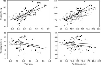
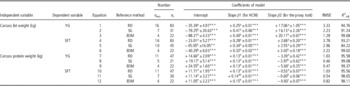
In the models relating carcass fat weight to each proxy trait (equations 1 to 6 in Table 3), the intercepts differed significantly when derived from the RD v. the SG or EOM data sets. The slopes associated with HCW were significantly lower when derived from the RD data set, whereas slopes associated with the proxy trait were significantly higher when derived from the EOM data set. These results indicate an interaction between HCW and proxy trait due to differences in animal characteristics between data sets. Therefore, the carcass fat calculated from EOM was higher on average than from RD (+2 kg) and SG (+15.8 kg) (Figure 1). Based on RMSE and R 2 adj, the best fit was noted for the EOM data set and the lowest one for the RD data set.
Relationships between carcass fat or protein weight and proxy traits (yield grade or subcutaneous fat thickness) derived from the rib dissection (RD, +), specific gravity (SG, Δ) and easily obtained measures (EOM, ●) data sets in cattle.

Quantitative relationships between the carcass fat or protein weight (kg, as the independent variables), and hot carcass weight (HCW, kg) with one proxy trait (yield grade (YG, 1 to 5) or subcutaneous fat thickness (SFT), mm) (as the dependent variables), accounting for the reference method used to determine carcass fat and protein (rib dissection (RD), specific gravity (SG), combination between easily obtained measures (EOM)) in cattle

n exp=number of experimental studies; n t=number of treatments.
NS=not significant: P>0.10, *P<0.05; **P<0.01; ***P<0.001.
a,b,cCoefficients followed by the same letter on the same column for the same independent and dependent variable (e.g. models from 1 to 3) are not significantly different at the 5% level (t-test).
Similarly, the models between carcass protein and proxy traits were significantly affected by the choice of reference method (Table 3). When considering YG as the proxy trait (equations 7 to 9 in Table 3), the reference method significantly affected the intercepts with the lowest value derived from the RD data set, and the highest from the EOM data set. The slopes associated with HCW remained similar whatever the reference method (at 0.13), but the slopes associated with YG were affected by the choice of the reference method. As a result, the weight of carcass protein calculated from RD was on average lower than from SG (−0.3 kg) and EOM (−1.8 kg) (Figure 1). When considering SFT as the proxy trait (equations 10 to 12 in Table 3), intercepts were similar across reference methods, but slopes associated with both HCW and proxy trait significantly differed. The differences in slopes resulted in higher calculated carcass protein weight from EOM than from RD (+2.1 kg) and SG (+2.9 kg) (Figure 1). Based on RMSE and R 2 adj, the best fit was noted for the EOM and SG data sets and the lowest one for the RD sub-data set.
Discussion
The different methods of determination of the chemical composition of carcass in cattle, referred here as the reference methods, are an important factor to consider when analyzing published results. Current results show that the amounts of carcass fat or protein predicted from a given proxy trait (YG or SFT) would significantly differ depending on the reference method associated to carcass fat or protein. Therefore, the amounts of carcass fat or protein vary with the method used for their measurement. Published results had already shown that carcass composition is not a homogeneous concept and depends on the method of measurement. In other words, none of the three reference methods considered here seems to be equivalent to the gold method of grinding and chemically analyzing the whole or half carcass. For example, Powell and Huffman (Reference Powell and Huffman1968) compared the chemical composition of the carcass measured from the whole carcass after grinding and chemical analysis, with that determined by RD (using the prediction equation developed by Hankins and Howe (Reference Hankins and Howe1946)) and by SG (using the prediction equation developed by Guenther et al. (Reference Guenther, Stuedemann, Ewing and Morrison1967)). A better accuracy was noted for RD than for SG. The same authors also measured a combination of EOM (HCW, SFT, ribeye area and kidney–pelvic–heart fat) and predicted carcass composition from three different equations (Murphey et al., Reference Murphey, Hallett, Tyler and Pierce1960; Cole et al., Reference Cole, Ramsey and Epley1962; Brungardt and Bray, Reference Brungardt and Bray1963). In all cases, the EOM method was even less accurate than the SG one.
Our results also suggest that proxy traits present different degrees of precision to estimate and ultimately predict the chemical composition of the carcass depending on the targeted reference method. However, the number of publications that were eligible and used in this study was not balanced across data sets. There was a very limited number of publications that used EOM as the reference method (n=4). As a result, the regression equations derived from the EOM data set always stood out and will not be further discussed. When considering the other reference methods (RD and SG), our results showed that they have a different degree of precision to estimate the carcass fat and protein weight. According to the RMSE of models, the best fit was calculated for SG as compared with RD. The SG data set was based on average on lighter and slower maturing animals and the range of variation of fat weight was higher in the SG than in the RD data set, as shown by the standard deviations (22.5 v. 14.5, Table 2). This might have contributed to a better fit. Indeed, SG is more accurate than RD to determine the chemical composition of the carcass when animals show a wide range of body fatness (Miller et al., Reference Miller, Cross, Baker, Byers and Recio1988). The R 2 between SG measurements and carcass fat was better across all age classes (calves, feeders, yearlings, steers and cows, R 2=0.68) than within each age class (R 2=0.13 to 0.44), revealing a low degree of accuracy intra classes. Also, SG has a good predictive capacity of body composition when the fat weight of the body is above 20% (Waldman et al., Reference Waldman, Tyler and Brungardt1969; Gil et al., Reference Gil, Johnson, Cahill, McClure and Klosterman1970), which was the case in the present data set.
What the current study has not been able to achieve, because of the limited data available, is to evaluate to which extent these results reflect the differences in animal characteristics between data sets, such as animal breeds, maturing rates and carcass weight. It is likely that the rates of fat deposition in each of the different fat tissues changed with animal types, and consequently modified the relationship between carcass composition and the dependent variables (HCW and proxy traits). The types of animals included in the data set were not representative of those used to develop the SG and RD methods. In our study, the fat contents of the carcass were similar in all three data sets (30% to 32%), whereas the protein content was lower in the RD v. the SG and EOM data sets (14.3 v. 16 and 15.5% on average, respectively). By contrast, the SG method initially developed by Garrett and Hinman (Reference Garrett and Hinman1969) was derived from older and heavier animals than the RD method developed by Hankins and Howe (Reference Hankins and Howe1946). In all cases, however, the current data sets differ widely from those used to develop the methods. The fact that the RD and SG methods were applied to animals that were not strictly representative of those used for method development may have contributed to the differenced in fit but may not be the only explanation. However, because of confounding factors between animal types and reference methods, detailed interpretation of results requires caution.
Conclusion
In conclusion, the amounts of carcass fat or protein predicted from a given proxy trait (YG or SFT) vary with the reference method used for measuring the carcass fat and protein.