1 Introduction
Pulsatile rough-wall turbulent pipe flow features throughout nature and engineering. For instance, the combined effect of unsteadiness and surface roughness can increase hydraulic losses in reciprocating pump piping systems (Shu, Burrows & Edge Reference Shu, Burrows and Edge1997) and augment arterial wall shear stress levels (Ciri et al. Reference Ciri, Bhui, Bailon-Cuba, Hayenga and Leonardi2018). Hence, the basic fluid dynamic properties of pulsatile rough-wall pipe flow are of great practical interest.
Non-pulsatile rough-wall turbulent pipe flow has been studied for many decades (Nikuradse Reference Nikuradse1933; Shockling, Allen & Smits Reference Shockling, Allen and Smits2006; Chan et al. Reference Chan, MacDonald, Chung, Hutchins and Ooi2015). Likewise, pulsatile smooth-wall pipe flow continues to receive attention across a range of forcing conditions (Manna, Vacca & Verzicco Reference Manna, Vacca and Verzicco2012; Papadopoulos & Vouros Reference Papadopoulos and Vouros2016; Cheng et al. Reference Cheng, Jelly, Illingworth, Marusic and Ooi2020), along with smooth-wall pulsatile turbulent channel flow (Scotti & Piomelli Reference Scotti and Piomelli2001; Weng, Boij & Hanifi Reference Weng, Boij and Hanifi2016), oscillatory open-channel flow (Kaptein et al. Reference Kaptein, Duran-Matute, Roman, Armenio and Clercx2019) and periodically forced Taylor–Couette turbulence (Verschoof et al. Reference Verschoof, te Nijenhuis, Huisman, Sun and Lohse2018). Pulsatile rough-wall turbulent channel flow has also been examined at three different forcing frequencies in past work by Bhaganagar (Reference Bhaganagar2008) using direct numerical simulation (DNS). In addition, unsteady rough-wall turbulent boundary layers have been studied extensively in geophysical contexts, e.g. tidally driven bottom boundary layers (Grant & Madsen Reference Grant and Madsen1986; Nayak et al. Reference Nayak, Li, Kiani and Katz2015) and oscillatory water flows over rough beds (Sleath Reference Sleath1987; Giménez-Curto & Lera Reference Giménez-Curto and Lera1996; Coleman, Nikora & Schlicke Reference Coleman, Nikora and Schlicke2008). In contrast, a dedicated study of pulsatile rough-wall turbulent pipe flow remains unavailable in the literature.
Considering the above studies, several questions regarding the fluid dynamic properties of pulsatile rough-wall turbulent pipe flow remain open. For instance, the validity of Townsend’s outer-layer similarity hypothesis (Townsend Reference Townsend1976) has yet to be tested. As a result, the existence and properties of the logarithmic layer in unsteady rough-wall turbulent pipe flow are unknown and need to be clarified. Likewise, little is known regarding the hydraulic properties of pulsatile rough-wall turbulent pipe flow. For example, the impact of unsteady forcing upon the Hama (Reference Hama1954) roughness function,  $\unicode[STIX]{x0394}U^{+}\equiv \unicode[STIX]{x0394}U/u_{\unicode[STIX]{x1D70F}}$, and the friction factor,
 $f\equiv 4\unicode[STIX]{x1D70F}_{w}/(\unicode[STIX]{x1D70C}U_{b}^{2}/2)$, has yet to be considered in detail. Here,
 $\unicode[STIX]{x0394}U$ is the downward shift in the mean streamwise velocity profile,
 $u_{\unicode[STIX]{x1D70F}}\equiv \sqrt{\unicode[STIX]{x1D70F}_{w}/\unicode[STIX]{x1D70C}}$ is the friction velocity,
 $\unicode[STIX]{x1D70F}_{w}$ is the total wall shear stress,
 $\unicode[STIX]{x1D70C}$ is density and
 $U_{b}$ is the bulk velocity. Without this knowledge, a priori predictions of roughness effects in unsteady turbulent pipe flows using conventional methods, i.e. assigning an equivalent value of the Nikuradse (Reference Nikuradse1933) sandgrain roughness and then estimating the drag penalty using a Moody (Reference Moody1944) chart, will simply not be possible.
To address these issues, we examine the fluid dynamic properties of pulsatile rough-wall turbulent pipe flow using DNS. Results for a set of three geometrically scaled roughness topographies are compared against an equivalent non-pulsatile dataset (Chan et al. Reference Chan, MacDonald, Chung, Hutchins and Ooi2018) at a single forcing condition, which, based on existing classifications, falls into the current-dominated (CD) very-high-frequency (VHF) regime. The principal interest here is to identify the key differences (and similarities) between the forced and unforced cases with the aim of clarifying the mean dynamics and the hydraulic properties of rapidly pulsating rough-wall turbulent pipe flow for the first time.
2 Numerical procedure
Direct numerical simulations of incompressible pulsatile rough-wall turbulent pipe flow were performed with the code CDP (Ham & Iaccarino Reference Ham and Iaccarino2004; Mahesh, Constantinescu & Moin Reference Mahesh, Constantinescu and Moin2004), following the computational workflow developed by Chan et al. (Reference Chan, MacDonald, Chung, Hutchins and Ooi2015). Code CDP is a finite-volume unstructured-grid flow solver, where diffusive and convective terms are advanced in time using a fully implicit Crank–Nicolson scheme, and mass conservation is enforced at each time step using the fractional-step method (Kim & Moin Reference Kim and Moin1985). A body-fitted mesh was used to explicitly resolve the rough walls, where impermeable no-slip boundary conditions were applied. The pipe has a length of  $L_{x}=4\unicode[STIX]{x03C0}R_{0}$, where
 $R_{0}$ is the mean radius, and pipe inlet–outlet plane was specified as a periodic boundary. Simulations were performed under constant mass-flux conditions and were set up such that the friction Reynolds number,
 $Re_{\unicode[STIX]{x1D70F}}\equiv u_{\unicode[STIX]{x1D70F}}R_{0}/\unicode[STIX]{x1D708}$ (where
 $\unicode[STIX]{x1D708}$ is kinematic viscosity) was equal to 540 for all cases considered here. The velocity components in the axial
 $(x)$, radial
 $(r)$ and azimuthal
 $(\unicode[STIX]{x1D703})$ directions are denoted
 $u_{x}$,
 $u_{r}$ and
 $u_{\unicode[STIX]{x1D703}}$, respectively, and
 $p$ is the fluctuating pressure. Note that the ‘spanwise’ (azimuthal) length in the pipe is measured along the arclength,
 $s=r\unicode[STIX]{x1D703}$. Viscous-scaled quantities are marked with a superscript
 $+$, e.g.
 $y^{+}=yu_{\unicode[STIX]{x1D70F}}/\unicode[STIX]{x1D708}$. The wall-normal direction is defined as
 $y\equiv (R_{0}-r-\unicode[STIX]{x1D716})$ where
 $\unicode[STIX]{x1D716}$ is the virtual origin offset. Following Chan et al. (Reference Chan, MacDonald, Chung, Hutchins and Ooi2015), the virtual origin of the wall
 $(y=0)$ is set to be
 $R_{0}$ – corresponding to a zero virtual origin offset
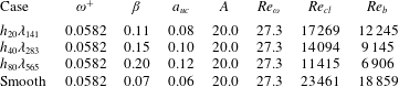
 $(\unicode[STIX]{x1D716}=0)$. A total of three pulsatile rough-wall simulations were performed, along with one pulsatile smooth-wall simulation. The simulation spatial resolution was chosen to match that of Chan et al. (Reference Chan, MacDonald, Chung, Hutchins and Ooi2018) – details are given in table 1, along with the temporal resolution and sampling period parameters for each case.
The roughness topography follows the two-dimensional cosine function
 $$\begin{eqnarray}\displaystyle R(x,\unicode[STIX]{x1D703})-R_{0}=h\cos (k_{x}x)\cos (k_{s}\unicode[STIX]{x1D703}), & & \displaystyle\end{eqnarray}$$
where  $h$ is the roughness semi-amplitude,
 $(k_{x},k_{s})=(2\unicode[STIX]{x03C0}/\unicode[STIX]{x1D706},2\unicode[STIX]{x03C0}R_{0}/\unicode[STIX]{x1D706})$ is the axial-azimuthal wavenumber pair and
 $\unicode[STIX]{x1D706}$ is the roughness wavelength, which is equal in the streamwise and azimuthal directions, i.e.
 $\unicode[STIX]{x1D706}_{x}=\unicode[STIX]{x1D706}_{s}=\unicode[STIX]{x1D706}$. A set of three geometrically scaled roughness topographies were considered in this study – the amplitude and wavelength of each surface were varied in proportion such that the ratio
 $h/\unicode[STIX]{x1D706}$ was held constant. As a result, the effective slope,
 $ES$, defined by Napoli, Armenio & De Marchis (Reference Napoli, Armenio and De Marchis2008) as the mean absolute streamwise gradient of the surface, also remains fixed, and, following Chan et al. (Reference Chan, MacDonald, Chung, Hutchins and Ooi2015), can be calculated using the formula
 $ES=(8/\unicode[STIX]{x03C0})h/\unicode[STIX]{x1D706}$ for the roughness topography considered here (equation (2.1)). A summary of the roughness parameters used throughout the course of this study is given in table 2.
Pulsation was imposed by prescribing an unsteady axial pressure gradient of the form
 $$\begin{eqnarray}\displaystyle \unicode[STIX]{x1D6F1}(t)=-{\displaystyle \frac{\text{d}\overline{p}}{\text{d}x}}[1+A\cos (\unicode[STIX]{x1D714}t)], & & \displaystyle\end{eqnarray}$$
where  $-\text{d}\overline{p}/\text{d}x$ is the mean axial pressure gradient,
 $A$ is the forcing amplitude and
 $\unicode[STIX]{x1D714}$ is the forcing frequency. Simulations were performed with an inner-scaled forcing frequency of
 $\unicode[STIX]{x1D714}^{+}\equiv \unicode[STIX]{x1D714}\unicode[STIX]{x1D708}/u_{\unicode[STIX]{x1D70F}}^{2}=0.0582$ and an amplitude ratio of
 $\unicode[STIX]{x1D6FD}\equiv U_{o}/U_{b}<1$, where
 $U_{o}$ is the amplitude of the oscillatory centre-line velocity and
 $U_{b}$ is the bulk velocity. The forcing amplitude,
 $A$, was specified such that
 $\unicode[STIX]{x1D6FD}=0.07$ for the smooth-wall case, and, in order of increasing roughness height,
 $\unicode[STIX]{x1D6FD}=\{0.11,0.15,0.20\}$ for the rough-wall cases. A summary of the forcing parameters used throughout the course of this study is given in table 3. The choice to focus on CD VHF regime was motivated by recent work regarding pulsatile smooth-wall pipe flow (Papadopoulos & Vouros Reference Papadopoulos and Vouros2016; Cheng et al. Reference Cheng, Jelly, Illingworth, Marusic and Ooi2020), as well as earlier work regarding pulsatile rough-wall turbulent channel flow (Bhaganagar Reference Bhaganagar2008), at comparable forcing conditions. Specifically, these past studies demonstrate that statistics of relative motion (e.g. velocity defect and Reynolds stress profiles) display an asymptotic approach towards a state of ‘frozen’ turbulence for forcing frequencies in excess of
 $\unicode[STIX]{x1D714}^{+}\gtrsim 0.04$, i.e. the pulsatile data collapse on to their non-pulsatile counterpart. The present study, therefore, complements this past work by examining the frozen turbulence phenomena in the context of CD VHF rough-wall turbulent pipe flow, and, in turn, the validity of Townsend’s outer-layer similarity hypothesis.
Simulation parameters for the rough- and smooth-wall cases including: friction Reynolds number,  $Re_{\unicode[STIX]{x1D70F}}$; number of points on the
 $r$–
 $\unicode[STIX]{x1D703}$ plane,
 $N_{r,\unicode[STIX]{x1D703}}$; number of points in the streamwise direction,
 $N_{x}$, and the number of points per roughness wavelength,
 $N_{\unicode[STIX]{x1D706}}$.
 $\unicode[STIX]{x0394}r_{w}^{+}$,
 $\unicode[STIX]{x0394}r\unicode[STIX]{x1D703}_{w}^{+}$, and
 $\unicode[STIX]{x0394}x_{w}^{+}$ are the mean viscous-scaled grid spacings at the wall. The largest cells are located in the central region of the pipe where
 $\unicode[STIX]{x0394}r^{+}\approx \unicode[STIX]{x0394}r\unicode[STIX]{x1D703}^{+}\approx \unicode[STIX]{x0394}x^{+}$. The viscous-scaled time step,
 $\unicode[STIX]{x0394}t^{+}$, the viscous-scaled forcing period,
 $T_{c}^{+}$, the number of completed cycles,
 $N_{c}$, and the number of sampling points per cycle,
 $N_{p}$, are also included. Line and symbol types are also defined for each case.

Roughness parameters including: axial-azimuthal wavenumber pair,  $(k_{x},k_{s})$; ratio of roughness semiamplitude to roughness wavelength,
 $h/\unicode[STIX]{x1D706}$; roughness wavelength to mean pipe radius,
 $\unicode[STIX]{x1D706}/R_{0}$; mean pipe radius to roughness semiamplitude,
 $R_{0}/h$; viscous-scaled roughness semiamplitude,
 $h^{+}$; wavelength,
 $\unicode[STIX]{x1D706}^{+}$; mean absolute height,
 $k_{a}^{+}$; root-mean-square roughness height,
 $k_{\text{rms}}^{+}$, and effective slope,
 $ES$.

Forcing parameters including: inner-scaled forcing frequency,  $\unicode[STIX]{x1D714}^{+}\equiv 2/l_{s}^{+2}$, where
 $l_{s}^{+}$ is the laminar Stokes length; ratio of the oscillatory centre-line velocity amplitude and bulk velocity,
 $\unicode[STIX]{x1D6FD}\equiv U_{o}/U_{b}$; ratio of the oscillatory centre-line velocity amplitude and centre-line velocity,
 $a_{uc}\equiv U_{o}/U_{cl}$, and the forcing amplitude,
 $A$ (equation (2.2)). The oscillation amplitude Reynolds number,
 $Re_{\unicode[STIX]{x1D714}}\equiv U_{o}^{2}/\unicode[STIX]{x1D714}\unicode[STIX]{x1D708}$, the bulk Reynolds number,
 $Re_{b}\equiv 2R_{0}U_{b}/\unicode[STIX]{x1D708}$, and centre-line Reynolds number,
 $Re_{cl}\equiv 2R_{0}U_{cl}/\unicode[STIX]{x1D708}$, are also included for reference.

Considering the periodic roughness topography (equation (2.1)) and unsteady forcing term (equation (2.2)), axial-azimuthal phase,  $(\unicode[STIX]{x1D719}_{x},\unicode[STIX]{x1D719}_{s})$, and temporal phase,
 $\unicode[STIX]{x1D719}_{t}$, are defined here as
 $(\unicode[STIX]{x1D719}_{x},\unicode[STIX]{x1D719}_{s},\unicode[STIX]{x1D719}_{t})\equiv 2\unicode[STIX]{x03C0}[(x/\unicode[STIX]{x1D706},s/\unicode[STIX]{x1D706},t/T_{c})~\text{mod}~1]$, where
 $T_{c}$ is the forcing period and
 $\text{mod}$ is the modulo operator. A triple phase-averaged (PA) quantity, say
 $\langle a\rangle$, is defined here as
 $$\begin{eqnarray}\displaystyle \langle a\rangle (\unicode[STIX]{x1D719}_{x},y,\unicode[STIX]{x1D719}_{s},\unicode[STIX]{x1D719}_{t})\equiv \lim _{N_{c}\rightarrow \infty }\frac{1}{N_{c}}\frac{1}{k_{x}}\frac{1}{k_{s}}\mathop{\sum }_{n=0}^{N_{c}-1}\mathop{\sum }_{p=0}^{k_{x}-1}\mathop{\sum }_{q=0}^{k_{s}-1}a(x+p\unicode[STIX]{x1D706},y,s+q\unicode[STIX]{x1D706},t+nT_{c}). & & \displaystyle\end{eqnarray}$$
A global-averaged (GA) quantity,  $\overline{a}$, is defined here as
 $$\begin{eqnarray}\displaystyle \overline{a}(y)\equiv \frac{1}{\unicode[STIX]{x1D713}(y)}\frac{1}{8\unicode[STIX]{x03C0}^{3}}\int _{0}^{2\unicode[STIX]{x03C0}}\int _{0}^{2\unicode[STIX]{x03C0}}\int _{0}^{2\unicode[STIX]{x03C0}}\langle a\rangle (\unicode[STIX]{x1D719}_{x},y,\unicode[STIX]{x1D719}_{s},\unicode[STIX]{x1D719}_{t})\,\text{d}\unicode[STIX]{x1D719}_{x}\,\text{d}\unicode[STIX]{x1D719}_{s}\,\text{d}\unicode[STIX]{x1D719}_{t}. & & \displaystyle\end{eqnarray}$$
In (2.4), the weighting function,  $\unicode[STIX]{x1D713}\equiv A_{f}(y)/A$, represents the ratio, at each wall-normal height, of the fluid-occupied area to the total area of the cylindrical shell. Since only fluid-occupied points contribute to spatially averaged quantities, all GA data considered herein correspond to an intrinsic average (Gray & Lee Reference Gray and Lee1977).
Considering equations (2.3) and (2.4), instantaneous field variables can be triple-decomposed as  $a(\boldsymbol{x},t)=\overline{a}(y)+\tilde{\hat{a}}(\unicode[STIX]{x1D719}_{x},y,\unicode[STIX]{x1D719}_{s},\unicode[STIX]{x1D719}_{t})+a^{\prime }(\mathbf{x},t)$, where
 $\tilde{\hat{a}}\equiv \langle a\rangle -\overline{a}$ is the triple PA oscillation and
 $a^{\prime }\equiv a-(\overline{a}+\tilde{\hat{a}})$ is the turbulent (or stochastic) fluctuation. The spatially averaged PA oscillation,
 $\hat{a}$, is defined here as
 $$\begin{eqnarray}\displaystyle \hat{a}(y,\unicode[STIX]{x1D719}_{t})\equiv \frac{1}{4\unicode[STIX]{x03C0}^{2}}\int _{0}^{2\unicode[STIX]{x03C0}}\int _{0}^{2\unicode[STIX]{x03C0}}\tilde{\hat{a}}\left(\unicode[STIX]{x1D719}_{x},y,\unicode[STIX]{x1D719}_{s},\unicode[STIX]{x1D719}_{t}\right)\text{d}\unicode[STIX]{x1D719}_{x}\,\text{d}\unicode[STIX]{x1D719}_{s}, & & \displaystyle\end{eqnarray}$$
and, finally, the spatially averaged PA quantity,  $\langle \overline{a}\rangle$, is defined here as
 $$\begin{eqnarray}\displaystyle \langle \overline{a}\rangle (y,\unicode[STIX]{x1D719}_{t})\equiv \overline{a}(y)+\hat{a}(y,\unicode[STIX]{x1D719}_{t}). & & \displaystyle\end{eqnarray}$$
3 Results
3.1 Amplitude ratio and phase lag analysis of axial velocity oscillations
First, it is useful to examine the relationship between the centre-line axial velocity oscillation,  $\hat{u} _{x,cl}$, and the sinusoidally varying pressure gradient,
 $\text{d}\hat{p}/\text{d}x$ (equation (2.2)). Following Mao & Hanratty (Reference Mao and Hanratty1986), the balance of oscillatory axial momentum along the pipe centre line under CD VHF forcing is described by the equation
 $$\begin{eqnarray}\displaystyle \frac{\text{d}\hat{u} _{x,cl}}{\text{d}t}=-\frac{1}{\unicode[STIX]{x1D70C}}\frac{\text{d}\hat{p}}{\text{d}x}, & & \displaystyle\end{eqnarray}$$
where the centre-line axial velocity oscillation is defined as  $\hat{u} _{x,cl}(\unicode[STIX]{x1D719}_{t})\equiv \langle \overline{u}_{x}\rangle (y=R_{0},\unicode[STIX]{x1D719}_{t})-\overline{u}_{x}(y=R_{0})$ (equation (2.6)). A solution of equation (3.1) for the time-harmonic pressure gradient equation (2.2) is
 $$\begin{eqnarray}\displaystyle \unicode[STIX]{x1D714}|\hat{u} _{x,cl}|\sin (\unicode[STIX]{x1D714}t+\unicode[STIX]{x1D6F7}_{cl})=\frac{1}{\unicode[STIX]{x1D70C}}\left|{\displaystyle \frac{\text{d}\hat{p}}{\text{d}x}}\right|\cos (\unicode[STIX]{x1D714}t), & & \displaystyle\end{eqnarray}$$
where  $|\hat{u} _{x,cl}|$ and
 $|\text{d}\hat{p}/\text{d}x|$ are the amplitude of the centre-line axial velocity oscillation and the oscillatory axial pressure gradient, respectively, and
 $\unicode[STIX]{x1D6F7}_{cl}$ is the phase angle at the pipe centre line. The variation of
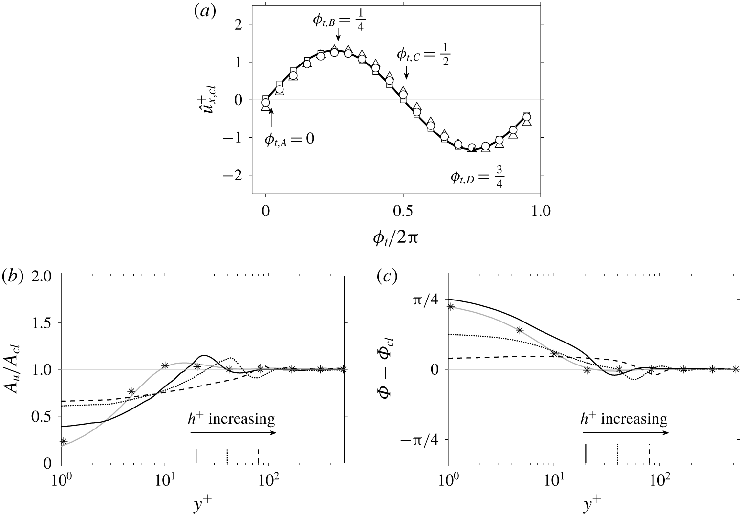
 $\hat{u} _{x,cl}$ throughout the forcing cycle is plotted in figure 1(a), along with data points for each case in table 2. The sinusoidal variation of
 $\hat{u} _{x,cl}$ indicates that
 $\unicode[STIX]{x1D6F7}_{cl}=\unicode[STIX]{x03C0}/2$ for both the smooth- and rough-wall data – in line with the form of equation (3.2). Whereas
 $\hat{u} _{x,cl}$ can be described by a fundamental mode, the validity of this approximation at other wall-normal heights is unclear. To this end,
 $\hat{u} _{x}$ was expanded as a Fourier series:
 $$\begin{eqnarray}\displaystyle \hat{u} _{x}(y,\unicode[STIX]{x1D719}_{t})=A_{u}(y)\sin [\unicode[STIX]{x1D714}t+\unicode[STIX]{x1D6F7}(y)]+\mathop{\sum }_{n=2}^{\infty }A_{u}^{n}(y)\sin [n\unicode[STIX]{x1D714}t+\unicode[STIX]{x1D6F7}^{n}(y)], & & \displaystyle\end{eqnarray}$$
where  $A_{u}(y)$ is the amplitude of the fundamental mode at each wall-normal location.
(a) Axial velocity oscillation at the pipe centre-line,  $\hat{u} _{x,cl}$, along with sinusoidal waveform
 $|\hat{u} _{x,cl}|\sin (\unicode[STIX]{x1D714}t)$ (——) for reference. Symbols correspond to DNS data and are defined in table 1. (b) Amplitude normalised by the centre-line amplitude,
 $A_{u}(y)/A_{cl}$. (c) Phase angle referenced against the centre-line value,
 $\unicode[STIX]{x1D6F7}(y)-\unicode[STIX]{x1D6F7}_{cl}$. Results for the Womersley (Reference Womersley1955) solution at matched forcing conditions also included for comparison
 $(\ast )$. Vertical lines on (b) and (c) indicate height of the roughness crests. All data scaled using the GA friction velocity,
 $u_{\unicode[STIX]{x1D70F}}$.

The wall-normal variation of  $A_{u}(y)$ normalised by its centre-line value,
 $A_{cl}$, is plotted in figure 1(b). For wall-normal locations greater than
 $y^{+}>100$, the rough- and smooth-wall data follow a horizontal line of unit amplitude. On the other hand, the amplitude ratio exhibits an overshoot in the vicinity of the roughness crests before decaying within the roughness canopy. The wall-normal variation of
 $\unicode[STIX]{x1D6F7}(y)$ referenced against its centre-line value,
 $\unicode[STIX]{x1D6F7}_{cl}$, is plotted in figure 1(c). Relative to the centre-line value, a negligible phase difference is observed for wall-normal locations greater than
 $y^{+}>100$ for both the smooth- and rough-wall configurations. As a result, the phase angle maintains its centre-line value of
 $\unicode[STIX]{x1D6F7}_{cl}=\unicode[STIX]{x03C0}/2$ (equation (3.2)) in the outer region of the flow, whereas, in the region below the roughness crests,
 $\unicode[STIX]{x1D6F7}$ decreases with increasing roughness height. A final observation based on figure 1(b,c) is the close match between the smooth-wall data and the Womersley (Reference Womersley1955) laminar solution at matched forcing conditions – a well-documented behaviour in pulsatile smooth-wall turbulent pipe flow, e.g. see recent work by Cheng et al. (Reference Cheng, Jelly, Illingworth, Marusic and Ooi2020).
Overall, figure 1 implies that, for wall-normal locations greater than  $y^{+}>100$, axial velocity oscillations are well approximated by the fundamental Fourier mode (equation (3.3)), regardless of the roughness topographies considered here (table 2). Hence, spatially averaged PA axial velocity profiles,
 $\langle \overline{u}_{x}\rangle \equiv \overline{u}_{x}+\hat{u} _{x}$ (equation (2.6)), are expected to retain their GA distribution in the outer region but with a periodic shift in response to the unsteady forcing. In what follows below, spatially averaged PA data are presented at the four phases marked on figure 1(a), namely, the peak-acceleration
 $(\unicode[STIX]{x1D719}_{t,A}=0)$, zero-acceleration
 $(\unicode[STIX]{x1D719}_{t,B}=1/4)$, peak-deceleration
 $(\unicode[STIX]{x1D719}_{t,C}=1/2)$ and zero-deceleration
 $(\unicode[STIX]{x1D719}_{t,D}=3/4)$ phases.
3.2 Assessment of Townsend’s outer-layer similarity hypothesis using PA data
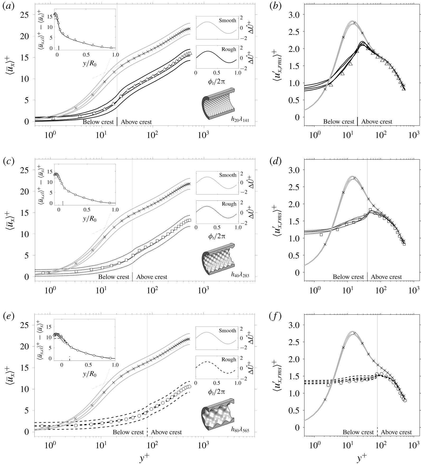
Spatially-averaged PA axial velocity profiles for case  $h_{20}\unicode[STIX]{x1D706}_{141}$ are plotted in figure 2(a), along with non-pulsatile rough-wall and smooth-wall data for reference. The first notable observation based on figure 2(a) is the preservation of a (nominal) logarithmic layer at each phase – implying that velocity profiles retain their self-similar functional form throughout the forcing cycle. The self-similar nature of the velocity profiles is clearer after recasting them into defect form, which, with reference to the top-left inset on figure 2(a), collapses the PA data onto a single curve, and on top of the results of Chan et al. (Reference Chan, MacDonald, Chung, Hutchins and Ooi2018), when plotted against
 $y/R_{0}$. A second notable observation based on figure 2(a) is that the log-laws of the rough- and smooth-wall flows oscillate with the same phase and amplitude – corroborating the preceding analysis of axial velocity oscillations (figure 1). Spatially-averaged PA axial velocity profiles for cases
 $h_{40}\unicode[STIX]{x1D706}_{283}$ and
 $h_{80}\unicode[STIX]{x1D706}_{565}$ are plotted in figures 2(c) and 2(e), respectively, and show the same trends in the outer region. These observations imply that the log-layer remains intact but with a periodic shift due to the unsteady forcing. Hence, the rough-wall log-law can be expressed in PA form as
 $$\begin{eqnarray}\displaystyle \langle \overline{u}_{x}^{+}\rangle (y,\unicode[STIX]{x1D719}_{t})=\unicode[STIX]{x1D705}^{-1}\log y^{+}+B-\langle \unicode[STIX]{x0394}U^{+}\rangle (\unicode[STIX]{x1D719}_{t}), & & \displaystyle\end{eqnarray}$$
where  $\unicode[STIX]{x1D705}$ is the von Kármán constant,
 $B$ is the intercept and
 $\langle \unicode[STIX]{x0394}U^{+}\rangle \equiv \unicode[STIX]{x0394}U^{+}+\unicode[STIX]{x0394}\hat{U} ^{+}(\unicode[STIX]{x1D719}_{t})$ is the PA Hama roughness function, defined as the difference between the GA smooth-wall and PA rough-wall centre-line velocities at matched flow conditions. For each case, the oscillatory Hama roughness function,
 $\unicode[STIX]{x0394}\hat{U} ^{+}$, achieves its maximum value at the zero-acceleration phase (
 $\unicode[STIX]{x1D6F7}_{t,B}=1/4$), following a transient favourable pressure gradient
 $(\text{d}\hat{p}/\text{d}x<0)$, whereas the opposite occurs at the zero-deceleration phase (
 $\unicode[STIX]{x1D6F7}_{t,D}=3/4$), following a transient adverse pressure gradient
 $(\text{d}\hat{p}/\text{d}x>0)$. In order of increasing roughness amplitude,
 $\unicode[STIX]{x0394}U^{+}=\{6.4,9.0,11.5\}$ for the pulsatile data – matching the past results of Chan et al. (Reference Chan, MacDonald, Chung, Hutchins and Ooi2018) to within 3 % for each case in table 2.
Spatially averaged PA velocity statistics including (a,c,e) axial velocity profiles,  $\langle \overline{u}_{x}\rangle$, and (b,d,f) axial r.m.s. profiles,
 $\langle u_{x,rms}^{\prime }\rangle$. Phase-averaged data are shown at the four phases marked on figure 1(a). Non-pulsatile data from Chan et al. (Reference Chan, MacDonald, Chung, Hutchins and Ooi2018) (symbols) and smooth-wall
 $(\times )$ data is included. Top-left inset panel shows the PA velocity defect profiles,
 $\langle \overline{u}_{x,cl}\rangle ^{+}-\langle \overline{u}_{x}\rangle ^{+}$, and top-right inset panels show the oscillatory component of the PA roughness function,
 $\unicode[STIX]{x0394}\hat{U} ^{+}$. Line and symbol types are given in table 1. Data are scaled by the GA friction velocity,
 $u_{\unicode[STIX]{x1D70F}}$.

In line with the PA velocity defect profiles inset on figure 2(a,c,e) the profiles of r.m.s. axial turbulence fluctuations shown in figure 2(b,d,f), also exhibit an invariance with respect to temporal phase in the outer region. In addition, the PA r.m.s. profiles closely follow the non-pulsatile data of Chan et al. (Reference Chan, MacDonald, Chung, Hutchins and Ooi2018), as well as the smooth-wall data, for each case in table 2. Such frozen behaviour is well-documented in past studies of smooth-wall pulsatile turbulent pipe flows. For instance, Papadopoulos & Vouros (Reference Papadopoulos and Vouros2016) demonstrated that PA turbulent intensity profiles relax onto their non-pulsatile counterpart for forcing frequencies in excess of  $\unicode[STIX]{x1D714}^{+}\approx 0.04$, noting that this behaviour demarcates the onset of the VHF regime. In addition, past work by Bhaganagar (Reference Bhaganagar2008) also showed that the modulation of turbulence in the outer region of pulsatile rough-wall channel flow decreases with increasing frequency and asymptotes to zero for a forcing frequency of
 $\unicode[STIX]{x1D714}^{+}=0.07$.
Overall, two key conclusions can be drawn from figure 2: (i) PA axial velocity profiles retain a self-similar functional form in the outer region, which can be described using a PA extension of the rough-wall log-law (equation (3.4)), and (ii) second-order turbulence statistics appear frozen in the outer region and collapse onto the non-pulsatile and smooth-wall data for all phases. Together, (i) and (ii) provide considerable evidence in support of Townsend’s outer-layer similarity hypothesis.
3.3 Hydraulic properties of pulsatile rough-wall turbulent pipe flow
The GA friction factor,  $\overline{f}$, and bulk Reynolds number,
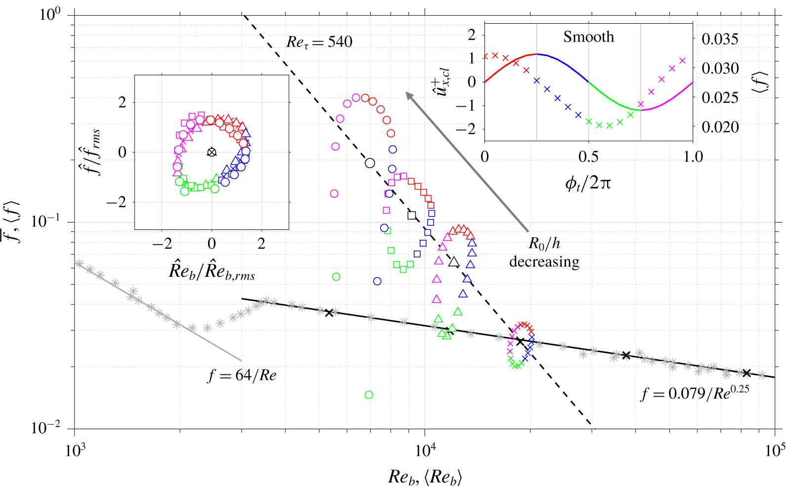
 $Re_{b}$, for each pulsatile case is plotted on a Moody (Reference Moody1944) chart in figure 3 and matches the steady data of Chan et al. (Reference Chan, MacDonald, Chung, Hutchins and Ooi2018) to within 3 % for each case listed in table 2. As expected,
 $\overline{f}$ increases as the ratio of mean pipe radius to the roughness height decreases, or, put in other words,
 $Re_{b}$ decreases with decreasing
 $R_{0}/h$. The spatially averaged PA friction factor,
 $\langle f\rangle$, and PA bulk Reynolds number,
 $\langle Re_{b}\rangle$, are also shown on figure 3 and form point-clouds that orbit the GA data. The former quantity is defined here as
 $\langle f\rangle =4\langle \unicode[STIX]{x1D70F}_{w}\rangle /(\unicode[STIX]{x1D70C}\langle U_{b}\rangle ^{2}/2)$, where
 $\langle \unicode[STIX]{x1D70F}_{w}\rangle$ is the total PA wall shear stress (which is composed of viscous and pressure drag components) and
 $\langle U_{b}\rangle$ is the PA bulk velocity. To aid the analysis of results, the PA data on figure 3 is colour-coded using the accelerating and decelerating intervals of the centre-line axial velocity oscillation,
 $\hat{u} _{x,cl}^{+}$ (see top-right inset figure 3). For the smooth-wall case, the phase lag between
 $\langle f\rangle$ and
 $\hat{u} _{x,cl}^{+}$ (figure 1a) is equal to
 $\unicode[STIX]{x03C0}/4$ (to within 3 %), indicating that the oscillatory component of the smooth-wall PA friction factor closely follows the Womersley (Reference Womersley1955) solution in the limit of VHF forcing. In addition, the phase lag between
 $\langle f\rangle$ and
 $\hat{u} _{x,cl}^{+}$ for cases
 $h_{20}\unicode[STIX]{x1D706}_{141}$ and
 $h_{40}\unicode[STIX]{x1D706}_{283}$ matches the smooth-wall value of
 $\unicode[STIX]{x03C0}/4$ to within 8 %. On the other hand, the phase lag angle for case
 $h_{80}\unicode[STIX]{x1D706}_{565}$ is equal to
 $\unicode[STIX]{x03C0}/6$, indicating that the time delay between the PA friction factor and centre-line velocity reduces by one third, relative to the smooth-wall case. A possible explanation for this behaviour is that pressure drag dominates viscous drag for case
 $h_{80}\unicode[STIX]{x1D706}_{565}$, and, as a result,
 $\langle f\rangle$ is unlikely to exhibit a Stokes-type behaviour in the fully-rough regime. A notable observation based on figure 3 is that, after computing the oscillatory component of the PA bulk Reynolds number,
 $\hat{Re}_{b}(\unicode[STIX]{x1D719}_{t})\equiv \langle Re_{b}\rangle -Re_{b}$, and friction factor,
 $\hat{f}(\unicode[STIX]{x1D719}_{t})\equiv \langle f\rangle -f$, then normalising by their respective r.m.s. values, the PA rough- and smooth-wall data follow a similar near-circular orbit (see
 $\hat{f}/\hat{f}_{rms}$ versus
 $\hat{Re}_{b}/\hat{Re}_{b,rms}$ plot, top-left inset panel figure 3). This result implies the orbital trajectory is insensitive to changes in surface topography and only depends on the applied forcing condition, at least for the four wall topographies considered in this study (table 2). It is worth noting, however, that in order of increasing roughness height,
 $\hat{f}_{rms}$ is equal to 33 %, 37 % and 67 % of
 $\overline{f}$ and
 $\hat{Re}_{b,rms}$ is equal to 8 %, 10 % and 13 % of
 $Re_{b}$ – indicating that increasing the size of the roughness elements leads to increasingly large variations in both
 $\langle f\rangle$ and
 $\langle Re_{b}\rangle$.
Moody chart. Global-averaged friction factor,  $\overline{f}$, and bulk Reynolds number,
 $Re_{b}$, shown as the symbols defined in table 1. Phase-averaged data is colour-coded using the accelerating (
 $\text{d}\hat{u} _{x,cl}^{+}/\text{d}\unicode[STIX]{x1D719}_{t}>0$ —— (red), —— (magenta)) and decelerating (
 $\text{d}\hat{u} _{x,cl}^{+}/\text{d}\unicode[STIX]{x1D719}_{t}<0$ —— (blue), —— (green)) intervals of the centre-line axial velocity oscillation (top-right inset). Top-left inset panel shows
 $\hat{f}/\hat{f}_{rms}$ plotted against
 $\hat{Re}_{b}/\hat{Re}_{b,rms}$. Laminar friction factor,
 $f=64/Re$ ——(grey), Blasius’ law,
 $f=0.079/Re^{0.25}$ ——, a line of
 $Re_{\unicode[STIX]{x1D70F}}=540$ (- - -) and Nikuradse’s smooth-wall data
 $(\ast )$ are included, along with smooth-wall nonpulsatile pipe flow DNS data at
 $Re_{\unicode[STIX]{x1D70F}}=\{180,360,540,1002,2003\}$ from Chin, Monty & Ooi (Reference Chin, Monty and Ooi2014) and Chan et al. (Reference Chan, MacDonald, Chung, Hutchins and Ooi2018)
 $(\times )$.

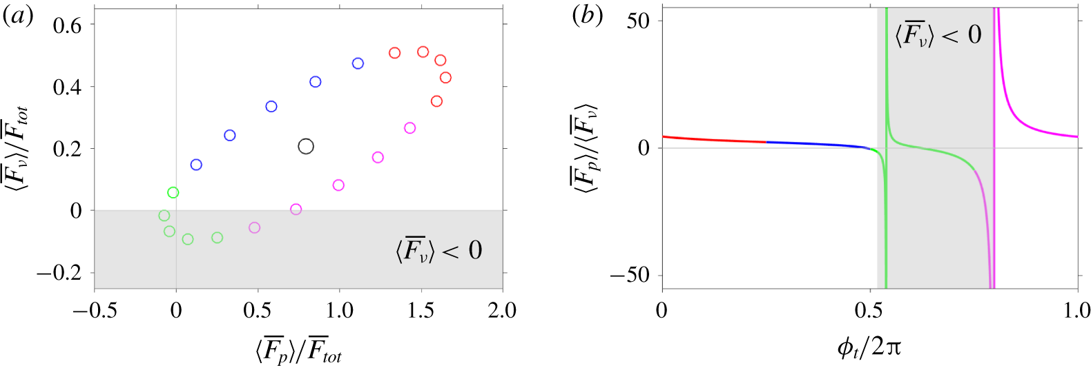
Analysis of PA pressure and viscous forces for case  $h_{80}\unicode[STIX]{x1D706}_{565}$. (a) Phase diagram of
 $\langle \overline{F}_{\unicode[STIX]{x1D708}}\rangle$ versus
 $\langle \overline{F}_{p}\rangle$, normalised by the total GA drag force,
 $\overline{F}_{tot}$. The elliptical point-cloud is centred around
 $(\overline{F}_{p},\overline{F}_{\unicode[STIX]{x1D708}})/\overline{F}_{tot}=(0.79,0.21)$ (○). (b) Ratio of PA pressure and viscous forces
 $\langle \overline{F}_{p}\rangle /\langle \overline{F}_{\unicode[STIX]{x1D708}}\rangle$ across the forcing cycle. Shaded grey rectangle denotes region where viscous shear stress becomes negative, i.e.
 $\langle \overline{F}_{\unicode[STIX]{x1D708}}\rangle <0$. Data is colour-coded in accordance with figure 3.

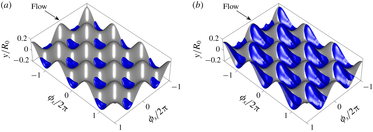
Isosurface of triple PA reverse flow  $(\langle u_{x}^{+}\rangle =-0.1)$ for case
 $h_{80}\unicode[STIX]{x1D706}_{565}$ at the (a) minimum (
 $\unicode[STIX]{x1D719}_{t}/2\unicode[STIX]{x03C0}=0.05$) and (b) maximum (
 $\unicode[STIX]{x1D719}_{t}/2\unicode[STIX]{x03C0}=0.55$) value of the PA friction factor,
 $\langle f\rangle$. Data is shown on a
 $(\unicode[STIX]{x1D719}_{x}\times \unicode[STIX]{x1D719}_{s})/2\unicode[STIX]{x03C0}=(3\times 2)$ doubly periodic subdomain. Data is scaled by the GA friction velocity,
 $u_{\unicode[STIX]{x1D70F}}$.

A further observation based on figure 3 is that  $\langle f\rangle$ becomes negative for phases on the range
 $0.50\lesssim \unicode[STIX]{x1D719}_{t}/2\unicode[STIX]{x03C0}\lesssim 0.60$ for case
 $h_{80}\unicode[STIX]{x1D706}_{565}$ (not visible on figure 3 due to the log-log format of the Moody chart). In order to associate specific mechanisms to this behaviour, the total PA drag force was decomposed as
 $\langle \overline{F}_{tot}\rangle =\langle \overline{F}_{\unicode[STIX]{x1D708}}\rangle +\langle \overline{F}_{p}\rangle$, where
 $\langle \overline{F}_{\unicode[STIX]{x1D708}}\rangle$ and
 $\langle \overline{F}_{p}\rangle$ are the spatially averaged PA viscous and pressure forces, respectively. Note that terms
 $\langle \overline{F}_{\unicode[STIX]{x1D708}}\rangle$ and
 $\langle \overline{F}_{p}\rangle$ both appear on the right-hand side of the PA hydrodynamic force balance equation, which can be expressed as
 $$\begin{eqnarray}\displaystyle \unicode[STIX]{x1D70C}\frac{\text{d}\langle U_{b}\rangle }{\text{d}\unicode[STIX]{x1D719}_{t}}=\unicode[STIX]{x1D70C}\langle \overline{F}_{x}\rangle V+\underbrace{\left\langle \iint _{\unicode[STIX]{x2202}S}-\overline{p}n_{x}\,\text{d}S\right\rangle }_{\langle \overline{F}_{p}\rangle (\unicode[STIX]{x1D719}_{t})}+\underbrace{\left\langle \iint _{\unicode[STIX]{x2202}S}\left(\unicode[STIX]{x1D708}\boldsymbol{n}\boldsymbol{\cdot }\unicode[STIX]{x1D735}\overline{\boldsymbol{u}}\right)\,\text{d}S\right\rangle }_{\langle \overline{F}_{\unicode[STIX]{x1D708}}\rangle (\unicode[STIX]{x1D719}_{t})}, & & \displaystyle\end{eqnarray}$$
where  $\langle \overline{F}_{x}\rangle$ is the streamwise driving PA pressure gradient, as in equation (2.2),
 $V$ is the volume occupied by the fluid,
 $\unicode[STIX]{x2202}S$ is the surface described by the roughness distribution (equation (2.1)) and
 $\boldsymbol{n}$ denotes the unit-normal vector. The phase diagram of
 $\langle \overline{F}_{\unicode[STIX]{x1D708}}\rangle$ versus
 $\langle \overline{F}_{p}\rangle$ normalised by the total GA drag force,
 $\overline{F}_{tot}(=\overline{F}_{\unicode[STIX]{x1D708}}+\overline{F}_{p})$, for case
 $h_{80}\unicode[STIX]{x1D706}_{565}$ is shown in figure 4(a). The data show that both
 $\langle \overline{F}_{p}\rangle$ and
 $\langle \overline{F}_{\unicode[STIX]{x1D708}}\rangle$ both attain negative values, and, as a result, the PA value of the total wall shear stress is also negative, i.e.
 $\langle \unicode[STIX]{x1D70F}_{w}\rangle <0$. One complication arising from this scenario is that the PA friction velocity,
 $\langle u_{\unicode[STIX]{x1D70F}}\rangle \equiv \sqrt{\langle \unicode[STIX]{x1D70F}_{w}\rangle /\unicode[STIX]{x1D70C}}$, is a complex number and, hence, the rationale behind inner scaling using the local friction velocity falls apart at these particular phases. The ratio of the PA pressure and viscous force,
 $\langle \overline{F}_{p}\rangle /\langle \overline{F}_{\unicode[STIX]{x1D708}}\rangle$, is plotted in figure 4(b) and reveals a rich array of unsteady flow physics not observed in the GA data (or in the past results of Chan et al. (Reference Chan, MacDonald, Chung, Hutchins and Ooi2018)). For instance, whereas the ratio of the GA forces is approximately four-to-one in favour of pressure drag, the ratio of the PA forces shows an altogether different picture. Notably,
 $\langle \overline{F}_{p}\rangle /\langle \overline{F}_{\unicode[STIX]{x1D708}}\rangle$ exhibits two discontinuities as the PA viscous force passes through a pair of zero-crossings – the first occurring at
 $\unicode[STIX]{x1D719}_{t}/2\unicode[STIX]{x03C0}=0.48$, when
 $\langle \overline{F}_{\unicode[STIX]{x1D708}}\rangle$ switches from positive to negative, and the second occurring at
 $\unicode[STIX]{x1D719}_{t}/2\unicode[STIX]{x03C0}=0.75$, when
 $\langle \overline{F}_{\unicode[STIX]{x1D708}}\rangle$ switches from negative to positive. The zero-crossings bound a region of negative viscous stress, i.e.
 $\langle \overline{F}_{\unicode[STIX]{x1D708}}\rangle <0$, which, as shown below, is related to flow recirculation within the roughness canopy.
In order to associate particular flow events to the variation of the PA pressure and viscous forces (figure 4), reverse-flow motions for case  $h_{80}\unicode[STIX]{x1D706}_{565}$ were examined. Isosurfaces of triple PA reverse flow at the phases corresponding to the maximum and minimum values of the total PA drag force are compared in figure 5. Whereas small reverse-flow pockets are visible within the roughness troughs at the former phase (
 $\unicode[STIX]{x1D719}_{t}/2\unicode[STIX]{x03C0}=0.05$, figure 5a), a significantly larger reverse-flow region engulfs the leeward-facing slopes at the latter phase (
 $\unicode[STIX]{x1D719}_{t}/2\unicode[STIX]{x03C0}=0.55$, figure 5b). A simple interpretation of this behaviour is as follows. As the flow accelerates, high-speed fluid rushes past the canopy, creating high-pressure regions on windward-facing slopes and (positive) viscous shear that hinders recirculation behind the crests (figure 5a). On the other hand, relatively low-speed fluid passes over the canopy as the flow decelerates, resulting in negative viscous stress (
 $\langle \overline{F}_{\unicode[STIX]{x1D708}}\rangle <0$), see shaded region on figure 4b), which promotes massive flow separation and recirculation downstream of the crests (figure 5b). Despite the large volume of reverse flow that develops within the canopy of case
 $h_{80}\unicode[STIX]{x1D706}_{565}$, and the fact that the total PA drag force becomes negative at
 $\unicode[STIX]{x1D719}_{t}/2\unicode[STIX]{x03C0}=0.55$ (figure 4a), it is worth noting that the PA bulk velocity remains positive for this phase (and all other phases), i.e.
 $\langle U_{b}\rangle >0$, due to the CD nature of the flow.
4 Conclusions
The flow physics of pulsatile rough-wall turbulent pipe flow were investigated for a set of three geometrically scaled roughness geometries at a single forcing condition using data obtained from DNS. The key findings of this work are given below.
Townsend’s outer-layer similarity hypothesis (Townsend Reference Townsend1976) is valid for the roughness-forcing combinations considered here. Specifically, the shape of the logarithmic region is preserved throughout the forcing cycle, and, as a result, the spatially averaged PA axial velocity profiles collapse onto a single curve after recasting them into defect form (figure 2a,c,e). Moreover, the ‘equilibrium’ log-law exhibits a periodic shift dictated by the PA Hama roughness function,  $\langle \unicode[STIX]{x0394}U^{+}\rangle$ (equation (3.4)), which oscillates with the same phase and amplitude for the cases considered here. In line with the PA velocity defect, the PA axial r.m.s. profiles are also invariant to temporal phase in the outer region and collapse on top of the smooth-wall data, as well as the non-pulsatile results of Chan et al. (Reference Chan, MacDonald, Chung, Hutchins and Ooi2018) (figure 2b,d,f). As a result, the pulsatile rough-wall pipe flow approaches a state of frozen turbulence – consistent with past work regarding smooth-wall pipe (Papadopoulos & Vouros Reference Papadopoulos and Vouros2016) and channel (Weng et al. Reference Weng, Boij and Hanifi2016) flows, as well as rough-wall turbulent channel flow (Bhaganagar Reference Bhaganagar2008), at similar CD VHF forcing conditions.
Whereas the hydraulic properties of the pulsatile and non-pulsatile rough-wall cases matched closely in the GA sense, the PA data revealed a rich array of unsteady flow physics not observed in the time-mean data. For instance, whilst the GA friction factor and bulk Reynolds number match to within 3 % for the forced and unforced cases, their PA values show clear differences (figure 3). Unsteady forcing had the most extreme impact upon case  $h_{80}\unicode[STIX]{x1D706}_{565}$, whose PA friction factor and bulk Reynolds number exhibited r.m.s. deviations of 67 % and 13 %, from their respective GA values. In addition, the PA friction factor for case
 $h_{80}\unicode[STIX]{x1D706}_{565}$ became negative at particular decelerating phases, which was explained in further detail by examining the phase portrait of the PA pressure and viscous forces (figure 4a), as well as their ratio (figure 4b), and, finally, by visualising regions of PA reverse flow in the roughness canopy (figure 5).
Overall, the results discussed here show that the major differences between pulsatile and non-pulsatile rough-wall pipe flow in the CD VHF regime are confined to the near-wall region, and, for the three roughness topographies considered here, show a strong dependency on the geometric scaling factor,  $h/\unicode[STIX]{x1D706}$ (table 2). Finally, whereas this work focused on a single forcing condition, the amplitude-frequency parameter space of pulsatile rough-wall pipe flow warrants further exploration. Ultimately, a frequency-based classification procedure for unsteady rough-wall pipe flow should be devised (and compared against its smooth-wall counterpart, e.g. see Cheng et al. (Reference Cheng, Jelly, Illingworth, Marusic and Ooi2020)), with the aim of extending this study across a broad range of forcing conditions.
Acknowledgements
The financial support of the Australian Research Council (ARC) is gratefully acknowledged. This work was supported by the ARC Linkage Project (LP150100233) and was undertaken with the resources and services from the National Computational Infrastructure, which is supported by the Australian Government.
Declaration of interests
The authors report no conflict of interest.