There is abundant evidence that public policies diffuse across the American states (e.g., Berry and Berry 1990, Mooney and Lee 1995). But why are one state's policymakers influenced by the policy choices of other states? Several explanations have been proposed, and two of the most common—policy learning and economic competition—reflect fundamentally different policymaking processes (Boehmke and Witmer 2004).
Some scholars maintain that states are influenced by the policy choices of other states because policymakers learn from the experiences of other states (e.g., Glick and Hays 1991, Mooney and Lee 1995). When confronted with a problem, decision makers simplify the task of finding a solution by choosing an alternative that has proven successful elsewhere (e.g., Simon 1997, Walker 1969). Most scholars who identify learning as the cause of interstate influence argue that diffusion of policy tends to be regional, with states looking primarily toward their neighbors or other nearby states for policies to emulate. Proximate states tend to share cultural, socioeconomic, and political characteristics that make them excellent “laboratories” for observing the likely effect of a policy choice (e.g., Walker).1
Not all learning models, however, are regional, as illustrated by Grossback, Nicholson-Crotty, and Peterson's (2004) model of diffusion among ideologically similar states.
Other researchers attribute the diffusion of policy to competition: state officials make policy choices to gain an economic advantage over proximate states. They compete to attract perceived “goods” (e.g., businesses, affluent taxpayers) and to deter perceived “bads” (e.g., loss of tax revenue, immigration of poor persons) (e.g., Bailey and Rom
2004, Ka and Teske
2002).
Regardless of whether scholars point to learning or competition (or both) to justify their models of interstate influence, the vast majority of empirical tests of such models have relied on a similar specification of influence—one that assumes that states are affected equally by all their neighbors, and unaffected by more distant states. For example, most recent tests of models of state diffusion have relied on event history analysis in which the dependent variable is the probability that a state not yet having a policy will adopt it, and one of the independent variables is the number (or proportion) of neighboring states that have previously adopted (e.g., Berry and Berry 1990, Ka and Teske 2002). It is predicted that a rise in the number of neighbors that have adopted a policy results in an increase in the probability of adoption.
When testing a learning model that emphasizes influence by proximate states, this specification of interstate influence—although simple—is quite reasonable, as states looking to nearby states for policy cues should be more likely to emulate a policy adopted by many neighbors than a policy adopted by few. However, the simple “number of neighbors” variable does not suffice for testing for the presence of economic competition. When interstate influence is due to competition, states' influences on each other should vary depending on the size and location of specific populations of individuals and firms within the states. For example, assume that the diffusion of lottery adoptions across states (observed by Berry and Berry [1990]) is due to competition, with states adopting lotteries for fear of losing revenues when residents travel to another state to play. If this were the case, a state that is surrounded by states with lotteries, but in which most people live over a hundred miles from a state border would be less likely to adopt a lottery than a state that has a single neighbor with a lottery, but most of its population in a city right on the border of that one state. Until recently, a model predicting this form of competition could not be tested because it was infeasible to measure the size and location of populations in all fifty states, especially over a multiyear period. But advances in geographic information systems (GIS) have made such measurements possible.
GIS have not seen wide use by political scientists (for exceptions, see Cho 2003 and Gimpel and Schuknecht 2003). However, we illustrate the value of GIS by applying them to test competition models of two state policy choices—the level of welfare benefits and the adoption of a lottery—for which scholars have posited that both learning and competition are responsible for policy diffusion. To allow a presentation of the applications in a relatively small amount of space, we modify models developed in earlier studies: Berry and Berry's (1990) model of state lottery adoptions, and Berry, Fording, and Hanson's (2003) welfare benefit model. Taken along with analyses of the original studies, which we contend are good tests for the presence of policy learning, our empirical analysis using GIS constitutes a critical test for whether the interstate influence detected by the original authors is due to learning or competition.
MEASURING THE CONCERN BY STATE OFFICIALS THAT MOTIVATES INTERSTATE COMPETITION
Berry and Berry's [hereafter B&B] (1990) model of the diffusion of the lottery proposes that the probability that a state without a lottery will adopt one is positively related to the number of its neighbors that have one, as states without lotteries adopt one to prevent the loss of revenues that occurs when residents cross the border to play other states' lotteries. Berry, Fording, and Hanson's [hereafter, BFH] (2003) welfare benefit model predicts that states try to set their benefits below those in surrounding states to discourage poor residents of other states from moving for more generous assistance. These models, although characterizing different policies, share an implicit presumption about the motivation of state officials to compete with nearby states. Both assume that a policy choice of a state—whether to adopt a lottery, or the size of its welfare benefit—is driven by the degree of concern of state officials about some form of behavior undertaken by citizens: a state resident buying a lottery ticket in another state or a poor person moving from another state for more generous public assistance. If we could observe these levels of concern, we could test these assumptions empirically.
Both models assume that state legislators and the governor are the principal officials involved in setting policy (B&B 1990, BFH 2003). One way to measure the degree of concern of these officials would be to survey them. However, obtaining responses from current office holders in every state would be difficult, and getting accurate assessments of the degree of concern of officials during previous legislative sessions would be virtually impossible. Lacking the ability to observe directly the level of concern of state officials, we use GIS to estimate Degree of concern. Although measurement details are different for the welfare and lottery applications, our basic strategy is the same:
- First, we identify the individuals at risk of engaging in the behavior of concern (buying a lottery ticket in another state, or moving to the state for better welfare benefits). We call these persons the population of concern. [For the lottery application, this consists of adults in the state living near a state with a lottery. For the welfare application, the population of concern of state A is all poor people who live (1) in other states with welfare benefits appreciably lower than state A's and (2) close to an appealing location in state A.]
- We then estimate, for each person in the population of concern, the individual's propensity to engage in the behavior of concern—a value assumed to be a function of geographic location. [For our lottery analysis, someone's propensity to buy a lottery ticket in another state is assumed to be inversely related to the distance of the person's residence from the nearest state with a lottery. For the welfare application, the propensity of a poor person from another state to move to state A for better welfare benefits is presumed to be a function of both the distance of the person's residence from an appealing location in state A and the difference between the benefit level in his or her current state and that available in state A.]
- Finally, given the estimated propensity to engage in the behavior of concern by individuals in the state's population of concern, the degree of concern of state officials is estimated by summing propensity values over all persons in the population of concern, and norming the sum by dividing by a measure of state population (for the lottery application, the state's adult population; for our welfare analysis, the state's poor population). This norming by state population is performed because the degree of concern reflected by any sum of individual propensity values should vary depending on the size of a state.
DISTINCT LEARNING AND COMPETITION HYPOTHESES
B&B (1990, 403) defend their prediction that the probability that a state will adopt a lottery is positively related to the number of previously adopting neighboring states by pointing to both policy learning (“previous adoptions by nearby states…yield important information about a [lottery's] effects”) and economic competition (“people living near the border…can cross [state lines] to purchase tickets”). We recognize that both learning and competition are plausible explanations for the diffusion of lottery adoptions, but offer distinct propositions consistent with the two explanations:
Lottery Learning Hypothesis: The probability that a state will adopt a lottery is positively related to the number of states bordering it that have previously adopted.
Lottery Competition Hypothesis: The probability that a state will adopt a lottery is positively related to the degree of concern of its officials about residents going to other states to play the lottery.
B&B's (1990) event history model of state lottery adoptions has as dependent variable whether a state without a lottery adopts one in a year and includes as independent variables a set of “internal determinants” (e.g., state fiscal health, proximity to a gubernatorial election) and the number of previously adopting neighboring states. B&B interpret the coefficient estimate for number of previously adopting states as a general test for the presence of regional diffusion (which they attribute to both learning and competition). In contrast, we view their empirical analysis as a test for the occurrence of policy learning, and fashion a distinct test for the presence of interstate competition by substituting measures of state officials' degree of concern about residents going to other states to play the lottery for the neighbors variable in B&B's model.
There have been many studies of interstate influence over welfare benefit levels (Bailey and Rom 2004; BFH 2003; Rom, Peterson, and Scheve 1998; Volden 2002). The vast majority of these have framed their empirical analysis as a test of the “race to the bottom” thesis: the supposition that state officials compete to keep their benefit levels below those in nearby states to discourage immigration by the poor. If the thesis is correct, one determinant of a state's benefit level should be the degree of concern of its officials about poor people moving to the state for better welfare benefits, a variable influenced not only by benefit levels in nearby states but also by the size and location of the poor population in these states. A few studies, however, have raised policy learning as an alternative explanation for states adjusting their benefits in response to their neighbors' changes in benefits (Allard 1998, Tweedie 1994). Setting a welfare benefit level is a difficult and controversial choice. Thus, policymakers may seek “benchmarks” for comparison, and benefit levels in neighboring states are an obvious and reasonable frame of reference. Consequently, when the benefit level in a state increases relative to the average benefit level in neighboring states, the state should decrease its benefit level in the following year (to bring it closer to that available in benchmark states). We believe that both learning and competition are plausible explanations for states' benefit levels being influenced by their neighbors', and we introduce hypotheses consistent with both explanations:
Welfare Learning Hypothesis: An increase in a state's welfare benefit relative to the average benefit in neighboring states prompts a decrease in the state's benefit in the following year.
Welfare Competition Hypothesis: An increase in the degree of concern by state officials about poor people in other states moving to the state for better welfare benefits prompts a decrease in the state's benefit in the following year.
The dependent variable in BFH's (2003) model of welfare benefits is a state's real (i.e., inflation-adjusted) Aid to Families with Dependent Children (AFDC) benefit level. One of its independent variables is the state's AFDC benefit level relative to the average benefit level in neighboring states in the previous year. The authors maintain that the coefficient for “benefit relative to neighbors” indicates the strength of interstate benefit competition.2
Most other studies of benefit competition also measure welfare benefits in real dollars (e.g., Bailey and Rom 2004; Figlio, Koplin, and Reid 1999; Rom, Peterson, and Scheve 1998; Saavedra 2000). This means that a failure to adjust benefits to compensate for inflation is equated with a decline in benefits. In contrast, Volden (2002) studies benefit competition with a logit model predicting whether a state increases its nominal benefit as a function of the proportion of neighboring states that have adopted a benefit increase.
We view BFH's coefficient estimate as testing the welfare learning hypothesis. To test the welfare competition hypothesis, we substitute measures of state officials' concern about welfare migration for “benefit relative to neighbors” in BFH's model.
Thus, our strategy for testing the lottery and welfare competition hypotheses requires us to construct measures of the degree of concern by state officials (about residents going to other states to play the lottery, and about poor people in other states moving to the state for better welfare benefits). We now describe our use of GIS to accomplish this task.
USING GIS TO ESTIMATE DEGREE OF CONCERN ABOUT THE LOSS OF LOTTERY REVENUE
Identifying the Population of Concern
Let D be the maximum distance (in miles) a person would be willing to travel to purchase a lottery ticket. Although D undoubtedly varies across individuals, to make our model tractable, we assume this value is constant.3
Below, we report evidence that our results are robust across a variety of assumptions about the value of D.
Thus, for any state,
s, without a lottery, we define the population of concern (those individuals at risk of going to other states to play the lottery) in a year as all adults in the state who live less than
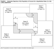
D miles from a state that had a lottery prior to the beginning of the year. The shaded region in
Figure 1 depicts the population of concern of a hypothetical state [S] within
D miles of five states, three of which have a lottery (T, U, and W) and two of which do not (R and V). Note that to obtain the shaded region, we form a band of width
D internal to the border of state S, but we exclude those sections of the band that are not within
D miles of a state with a lottery. The most extreme southeast corner of state S is in the shaded region by virtue of being within
D miles of nearby (but non-neighboring) state W.
Schematic Depiction of the Population of Concern for a Hypothetical State, S, in the Lottery Application
Although it is theoretically feasible to use GIS to identify the location of all persons in each state's population of concern, the individual-level residential data necessary for our application are as of yet unavailable. Thus, we make the simplifying assumption that each person in a county is at the same location. This means that although the individual is the conceptual unit of analysis, our empirical analysis with GIS is conducted using counties as the units for computation.4
Clearly, the smaller the units, the more accurate would be our calculation of the degree of concern. We chose the county because it is the lowest level of aggregation at which population counts are available annually for our period of analysis. A smaller unit, like the Census tract, is not feasible because a large portion of the country was not tracted for part of our period of analysis (i.e., for years before 1980) and boundaries for tracts change over time.
In the following, we consider alternative assumptions about the point within a county at which its residents are located.
Measuring the Propensity of Individuals to Engage in the Behavior of Concern
For each individual, i, in the population of concern of state s, we use GIS to determine the distance, di, of that person from the closest state that had a lottery prior to the beginning of the year. [Note that we employ the subscript i to denote a characteristic of an individual; subscripts s and c indicate a characteristic of a state or county, respectively.] Figure 1 depicts the value of di for an individual who resides at the dot near the western border of state S. Although in theory, we could measure distance with as much precision as desired using GIS, if measurement were highly precise (e.g., distance were measured to the nearest mile), there would be a dramatic increase in the memory and time required for our computer program. Thus, we measure distance to the nearest multiple of ten miles (i.e., 0 miles, 10 miles, 20 miles, etc.) [See Section I of the unpublished supplement for a detailed description of how we use GIS to measure distance from the nearest state with a lottery.]
For each individual, i, in the population of concern, let the propensity to play another state's lottery be defined by
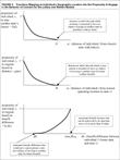
where f(di) is a decreasing monotonic function of di that maps a distance of 0 into a propensity score of 1 and a distance of D into a propensity of 0, and has declining slope as di increases, as illustrated in the top panel of Figure 2. Thus, for someone living right on the border of a state with a lottery (i.e., for whom di=0), the propensity to play another state's lottery is 1.00 (the maximum value on the propensity scale). We assume that as distance from the border rises (i.e., as di increases), propensity to play another state's lottery declines, but the rate of decline decreases as distance gets larger. This assumption reflects a belief that a marginal increase in distance has a greater impact on propensity when someone leaves near the state border than when someone lives farther away. For example, persons living 0 and 20 miles from a state with a lottery should have propensities to play the neighbor's lottery that differ more than persons living 80 and 100 miles from the border. When distance from the border reaches D, the propensity to play another state's lottery subsides to zero (the minimum value on the scale). Thus, although the population of concern consists of all adults living within D miles of a state with a lottery, not everyone in this population is assumed to be of equal concern to policymakers. In effect, the concern of state officials about someone going to another state to play the lottery declines as the distance of the person's residence from the nearest state with a lottery increases.
Functions Mapping an Individual's Geographic Location into the Propensity to Engage in the Behavior of Concern for the Lottery and Welfare Models
Aggregating Individual Propensities to Compute Degree of Concern
Let the degree of concern about residents going to other states to play the lottery for a state in a year be zero if the state has its own lottery in that year. Then, for any state, s, that does not have a lottery, calculate the degree of concern by adding up the propensity to play another state's lottery over all persons in the population of concern of state s, and dividing the sum by the state's adult population:
So calculated, a score of 1 for degree of concern indicates the hypothetical condition in which every adult in a state without a lottery lives right at the border of a state with a lottery; if half the adults in the state lived right at the border and the other half lived more than D miles away, degree of concern would be .50. At the other extreme, degree of concern would be zero if no adult lived less than D miles from a state with a lottery, or if the state already had its own lottery during the year of measurement.
USING GIS TO ESTIMATE DEGREE OF CONCERN ABOUT WELFARE MIGRATION
Estimating the degree of concern about welfare migration is more complex than estimating the degree of concern about residents going to other states to play the lottery. We assume that an individual's propensity to play another state's lottery is a function of just one variable: his or her distance from the nearest state with a lottery. But we assume that a poor person's propensity to move to a state for better welfare benefits is a function of two factors: the distance of the person from an appealing location in the state and the benefit increase for which the person would be eligible.
Identifying the Population of Concern
Let M be the maximum distance (in miles) a poor person would be willing to move for better welfare benefits. Let Δ B be the minimum benefit difference in dollars that would motivate a poor person to move for greater welfare benefits.5
As with D in the lottery model, our application assumes M and Δ B are constant across individuals. But below, we report evidence of the stability of our findings across alternative assumptions about these values.
Given these definitions of
M and Δ
B, the population of concern for state
s (those poor persons at risk of moving to state
s for better welfare benefits) in a year can be defined as all poor persons in other states (neighboring or not) who live (1) within
M miles of an appealing location in state
s, and (2) in a state that has a welfare benefit at least Δ
B dollars lower than state
s's in the previous year.
We operationalize an “appealing location” as a city with an absolute population greater than p, and test models making varying assumptions about the value of p. One assumption is that p is zero. This implies that the poor are “location neutral”; they perceive any location as adequate if it is close enough and the welfare benefit there is sufficiently large. Most versions of the race to the bottom thesis presume that the poor are single-minded in pursuit of more generous welfare assistance (e.g., Bailey and Rom 2004; Rom, Peterson, and Scheve 1998). If this were correct, then the assumption that p equals zero would be reasonable. However, an alternative assumption is that p is substantially greater than zero, with poor persons having a clear preference for urban areas over rural ones. This is consistent with a belief that when poor persons move they choose a location that provides both generous welfare benefits and good opportunities for employment (Schram, Nitz, and Krueger 1998).
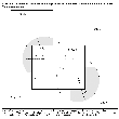
Figure 3 illustrates the population of concern for a hypothetical state, S. States T and W have welfare benefits appreciably lower (i.e., at least Δ B dollars lower) than state S's; states U and V have benefits either higher than those of state S or lower than S's but by an amount less than Δ B dollars. State S has two (appealing) cities with population greater than p, the locations of which are denoted by dots. The two circles are centered at these dots and have radius M. Thus, the circles represent persons living within M miles of an appealing location in state S. The shaded region represents the subset of the population within the circles that reside in states with welfare benefits appreciably (i.e., at least Δ B dollars) lower than state S's. Therefore, poor persons residing in the shaded area constitute the population of concern of state S. Note that poor individuals in states U and V who live within the circles are not in the population of concern because benefit levels in these two states are not at least Δ B dollars lower than the benefit in state S. As with our lottery application, individual-level residential data for conducting our welfare analysis are not available. Thus, we again assume that all persons in a county are at the same location, thereby permitting measurement of the degree of concern using county-level data.
Schematic Depiction of the Population of Concern for a Hypothetical State, S, in the Welfare Application
Measuring the Propensity of Individuals to Engage in the Behavior of Concern
For each individual in the population of concern of state s, we use GIS to determine the distance, mi, of that person from the nearest appealing location in state s. [Figure 3 shows the value of mi for an individual who resides at the asterisk in the southwest section of state T.] For each of these persons, let the propensity to migrate based on distance be defined by
where g(mi) is a decreasing monotonic function of mi that maps a distance of 0 into a propensity score of 1 and a distance of M into a propensity of 0, as depicted in the middle panel of Figure 2. Similarly to f(di) in the lottery model, g(mi) has declining slope as mi increases (to reflect an assumption that a marginal increase in distance has a smaller impact on propensity to migrate as distance gets larger).
Next, for each person, i, in the population of concern of state s, determine the benefit difference, Δ bi; this is defined as the welfare benefit in state s minus the welfare benefit in i's home state. Let max Δ b(M) be the maximum benefit increase (in absolute dollars) that can be achieved by an interstate move of no more than M miles during any year in the period of analysis. For each individual, i, in the population of concern, let the propensity to migrate based on benefit difference be defined by
where h(Δ bi)—depicted in the bottom panel of Figure 2—is an increasing monotonic function of Δ bi that maps a benefit difference ofΔ B into a propensity score of 0 and a benefit difference of maxΔ b(M) into 1, and has increasing slope as Δ bi increases.
In a final individual-level calculation, for each person, i, in the population of concern of state s, we determine the propensity to migrate for better welfare benefits:
Because both terms on the right side can range from zero to one, their product—the propensity to migrate for better welfare benefits—is confined to the same range. It is designed to be high only when both the propensity to migrate based on distance and the propensity to migrate based on benefit difference are high. For a poor person living (a) in a state with a benefit level max Δ b(M) lower than state i's and (b) zero miles from an appealing location in state s, the propensity to migrate for better welfare benefits would be 1.00 (the maximum value of the propensity scale). Someone who lives M or more miles from an appealing location in state s would have a score of zero (the minimum value on the scale) regardless of the benefit level available in his or her home state.
Aggregating Individual Propensities to Compute Degree of Concern
If state s's population of concern in a year is the empty set, let its degree of concern about welfare migration be zero. For other state-years, calculate the degree of concern by summing the propensity to migrate for better welfare benefits over all persons in the population of concern, and then dividing by the poor population of state s:
Defined this way, degree of concern equals zero if there are no “appealing locations” in state s, if there are no poor persons in other states who live within M miles of an appealing location in state s, or if there are no nearby states with a benefit level at leastΔ B dollars lower than state s's.
CONSTRUCTING MULTIPLE INDICATORS OF DEGREE OF CONCERN FOR THE LOTTERY AND WELFARE ANALYSES
Several parameters must be assigned specific values before our degree of concern variables can be measured using GIS. For the lottery model:
- D, the maximum distance (in miles) a person would be willing to travel to purchase a lottery ticket.
For the welfare model:
- p, the minimum population size for a city to be appealing to the poor;
- M, the maximum distance (in miles) a poor person would be willing to move for better welfare benefits; and
- Δ B, the minimum benefit difference (in dollars) that would motivate a poor person to move for better welfare benefits.
Because of theoretical uncertainty about the appropriate values for D, p, M, and Δ B, we construct our indicators of degree of concern using multiple values for these parameters, so that we can test the robustness of our empirical results to assumptions that are, to some degree, arbitrary. We employ four different values of the minimum population for a city to be appealing to the poor [p] (0; 100,000; 200,000 and 500,000),6
Because 1980 is the closest decennial Census year to the midpoint of the time periods we examine, we determine the cities surpassing the various population thresholds (p) using 1980 Census data.
three different values of the minimum benefit difference required to motivate a move [Δ
B] [100, 150, and 200 real (
1995) dollars, measured using Berry, Fording, and Hanson's (
2000) state cost of living index as a deflator], four different values of the maximum distance someone will travel to buy a lottery ticket [
D] (100, 150, 160, and 170 miles), and four different values of the maximum distance someone will move for better welfare benefits [
M] (150, 160, 170, and 220 miles). We calculate that max Δ
b(M)—the maximum benefit increase that can be achieved by an interstate move of no more than
M miles during any year in the period of analysis—is 878 real [1995] dollars for all four values of
M.
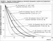
Each value of D and M, however, specifies only a maximum distance that a person is willing to travel to buy a lottery ticket or move for better welfare benefits. For each value of D, we must specify a function, f(di), that maps each distance smaller than D into a value for the propensity to play another state's lottery; and for each value of M we must specify a function, g(mi), that maps each distance smaller than M into a value for the propensity to migrate based on distance. Figure 4 plots these functions and presents their equations. Although three of the values for D and M—150, 160, and 170 miles—seem quite similar, the overall functions associated with these values are quite different. Indeed, the substantially different rates of descent of the functions associated with these values make it so the distance at which the propensity to engage in the behavior of concern drops below .10 varies substantially across the functions: when D or M is 150 miles, this distance is 56 miles; when D or M is 160, the distance is 86 miles; and when D or M is 170, it is 117 miles.
Specific Functions Mapping an Individual's Geographic Location into Propensity to Engage in the Behavior of Concern
For each value of Δ B (the minimum benefit difference that would motivate a move), we specify a different functional form for h(Δ bi), the function that maps each benefit difference [Δ bi] into a value for the propensity to migrate based on benefit difference. Each of these functions maps Δ B ($100, $150, or $200) into a score of zero, and increases monotonically, mapping maxΔ b(M) (the maximum achievable benefit increase, $878) into a propensity value of 1. Figure S-1 in our unpublished supplement plots these functions and shows their equations.
As noted earlier, given the lack of availability of individual-level data, we assume that all persons in a county are at the same location. Therefore, to operationalize degree of concern, we must designate a specific point within a county as the assumed location of its population. Our goal is to pick a location that yields estimates of the degree of concern that are close to the values we would obtain if we were able to construct a measure taking into account the exact location of each individual. Because we cannot determine with certainty the best location, we construct measures of the degree of concern for the lottery and welfare applications assuming both (1) that all persons in a county are at its geographic center, and (2) that all persons in a county are at the center of the city with the largest population. For a county with one dominant city, a degree of concern measure based on the center of the largest city is a good choice. However, when population is more evenly dispersed, an indicator based on the geographic center of the county seems superior. Although both versions of the measure have their theoretical advantages, in practice there is little difference between the two. Across a large number of measures of degree of concern making different assumptions about the values of D, p, M, and Δ B (all 52 measures for which results are reported in Tables 1 or 2, or in Tables S-1 or S-2 in our unpublished supplement), the correlation between the “geographic center” version of the measure and the “largest city” version always exceeds .98.
This result, however, does not indicate whether our measures of degree of concern yield scores similar to those that would be obtained if we were to employ the individual as the unit of analysis. To investigate this, we construct measures of the degree of concern making two different extreme assumptions about the location of population within counties. One set of measures presumes that all individuals are at the location in a county closest to the point of attraction to those in the population of concern (i.e., a state with a lottery, or a place that is appealing to the poor). The other set assumes that all persons are at the location in the county farthest from the point of attraction. Across a large number of indicators of the degree of concern, the average correlation between the “closest point” version of the measure and the “farthest point” version is .94. [Half the 52 correlations exceed .98; all but 9 are greater than .90; the lowest is .68.] Because the two maximally divergent assumptions yield measures that correlate very highly, it is very unlikely that the precise location of individuals within counties has a significant impact on the indicators we construct. This gives us confidence that the county is a unit of analysis small enough to produce measures of the degree of concern that are very likely to be close to the ones we would obtain if we knew the precise location of each individual in the population of concern. In all empirical tests that follow, we employ measures of degree of concern assuming that all persons in a county live at its geographic center.
For the lottery application, each of the four functions for f(di) yields a distinct measure of the propensity to play another state's lottery and ultimately a distinct value for degree of concern about residents going to other states to play the lottery. For our welfare application, using all combinations of the four values for p, the three functions for h(Δ bi), and the four functions for g(mi) yields 48 indicators of the propensity to migrate for better welfare benefits and ultimately, the degree of concern about welfare migration.7
The computation of degree of concern for our lottery analysis requires county counts of adult population (for each year during the period of analysis, 1964–86). Using population age 18 or older would be ideal because the vast majority of states limit sales of lottery tickets to this age group, but data constraints mandate that we employ population twenty or older. The calculation of degree of concern for our welfare analysis requires county counts of poor population (for each year during the period 1961–90). We obtained 1960 Census adult population data (Haines 2005) and annual estimates for the period 1970–90 (U.S. Bureau of the Census 2004); values for years between 1960 and 1970 were calculated using linear interpolation. Poverty counts for Census years 1960, 1970, 1980 and 1990 were obtained from Rural Policy Research Institute (2003), and values for intercensal years were estimated via linear interpolation between Census values.
We use ArcGIS 9.0 software (Environmental Systems Research Institute 2004) to construct our degree of concern indicators, but our calculations could be done with virtually any GIS software. We describe our GIS measurement procedure in greater detail in our unpublished supplement.
EMPIRICAL TESTS OF THE LOTTERY LEARNING AND COMPETITION HYPOTHESES
We test the lottery learning hypothesis by replicating the estimation of B&B's (1990) discrete event history model, which has as dependent variable whether a state adopts a lottery in a year, and includes among the independent variables the number of previously adopting neighbors. In particular, we estimate the model B&B report in the right-most column of their Table 1 (p. 406). To test the lottery competition hypothesis, we substitute each of our four measures of degree of concern for the number of previously adopting neighbors. To allow for duration dependence (i.e., to permit the probability of adoption of a lottery to vary over time), we also add a time counter to each equation (Buckley and Westmoreland 2004).8
This time counter is 1 in 1964 (the first year of analysis), 2 in 1965,… and 23 in 1986 (the last year of analysis). Note that we also estimated equations including dummy variables for years (as suggested by Beck, Katz, and Tucker [1998]). The estimated effects of degree of concern and number of previously adopting neighbors are very similar regardless of which approach to allow for duration dependence is used; thus, we report results for the more parsimonious specifications with a single time count variable.
We estimate each equation with probit, using the same 901 annual observations of the 48 contiguous states for 1964 through 1986 employed by B&B, but we compute robust standard errors—clustering by state to allow for dependence of observations within states.
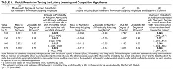
The learning hypothesis receives empirical support, but due to the addition of the time counter, the estimated effect of number of previously adopting neighbors is somewhat smaller than reported in B&B's article. The coefficient for number of previously adopting neighbors (MLE=0.135), although failing a test of statistical significance at .05, is significantly positive at the .10 level (one-tailed test; Z=1.29).
Results regarding the competition hypothesis (i.e., coefficient estimates for degree of concern when it is substituted for number of previously adopting neighbors) are summarized in columns 2 through 4 of Table 1. The maximum likelihood estimates of the coefficients for degree of concern (see column 2) are positive as predicted, and each is significant at the .05 level.9
Although the fit of our lottery model is fairly similar across analyses assuming different functions, f(d), mapping distance from the closest state with a lottery to the propensity to play another state's lottery, if fit had been substantially better using one of these functions, this might have provided insight into state officials' perceptions of how far people are willing to travel to play the lottery.
When the degree of concern about residents going to other states to play the lottery increases from its fifth percentile value in the sample to its ninety-fifth percentile value (and all other independent variables in the model are held constant at the mean), the probability that the state will adopt a lottery in a given year is estimated to increase by somewhere from .021 to .027 (depending on the value assumed for
D; see column 4).
10 This predicted increase in the probability of adoption is also statistically significant in two of the four versions of the model, as the 95% confidence interval for the estimated change in probability excludes zero for these models. For the other two versions, the 95% confidence interval just barely extends into the negative range (no further than −.001).
Although such probability differences may seem small, they are appreciable, given how rare lottery adoptions are during our period of analysis: the estimated probability that a state without a lottery will adopt one in a year is .030 (27 adoptions out of 901 observed cases). Thus, empirical analysis of lottery adoptions is consistent with both the competition and learning hypotheses, but support for the competition hypothesis is somewhat stronger. Yet because number of previously adopting neighbors and degree of concern are highly correlated—between .72 and .86, depending on which of the four versions of the latter variable is used—models in which just one of these variables is included may indicate an effect of that variable when none is present because the variable is picking up the true effect of the excluded variable.
A more definitive test of the two hypotheses can be achieved by including both degree of concern and number of previously adopting neighbors in the same model. If diffusion occurs strictly because of learning (and interstate competition plays no role whatsoever), the relationship between number of previously adopting neighbors and the probability of an adoption should survive a control for degree of concern, but the relationship between degree of concern and adoption probability should decline to near zero when number of previously adopting neighbors is added to the model. In contrast, if diffusion were solely a result of competition (and learning were not a factor), the relationship between degree of concern and the probability of adoption should survive a control for number of previously adopting neighbors, but the relationship between the neighbors variable and the probability of adoption should disappear when controlled for the effect of degree of concern.
Columns 5 through 9 of Table 1 present results when we include both number of previously adopting neighbors and degree of concern in our models. Observe that with degree of concern included, the coefficient estimate for number of previously adopting neighbors declines to near zero (indeed becomes slightly negative) in all four versions of the model (see column 5). However, we can see that the estimates of the coefficients for degree of concern survive a control for number of previously adopting neighbors: indeed the MLEs for degree of concern increase somewhat when number of neighbors is added to the model (compare columns 7 and 2). Similarly, the estimates of the effect of degree of concern on the probability of adoption increase for all four values of D when number of previously adopting neighbors is added (compare columns 9 and 4). Although point estimates of the effect of degree of concern increase in magnitude when number of previously adopting neighbors is included, Z statistics for the MLEs for degree of concern decrease (compare columns 8 and 3) and the width of confidence intervals for predicted changes in the probability of an adoption widen (compare columns 9 and 4). This is likely due to the strong correlation between number of previously adopting neighbors and degree of concern. Thus, there is compelling evidence that the interstate influence leading to the diffusion of the lottery results from competition—fear by state officials of losing revenues to neighboring states—rather than policy learning.11
Additional support for the claim that the diffusion of the lottery is due to competition rather than learning is derived from a statistical test developed by Davidson and MacKinnon (1993) and implemented by Greene (1995, 422). For all four values of D, conceiving of the equation including number of previously adopting neighbors and the equation including degree of concern as rival models, when the model involving number of neighbors is treated as the null, it is easily rejected in favor of the model including degree of concern (with t-ratios ranging in magnitude from 2.33 to 3.13). However, when the model including degree of concern serves as the null, it cannot be rejected for any value of D (t is always less than 0.22).
EMPIRICAL TESTS OF THE WELFARE LEARNING AND COMPETITION HYPOTHESES
We test the welfare learning hypothesis by replicating the estimation of BFH's original model, which has as dependent variable a state's AFDC benefit in a year (i.e., its maximum monthly AFDC payment [in real dollars] for a family of four with no income), and includes among the independent variables a state's benefit relative to the average benefit in neighboring states in the previous year (for short, “benefit relative to neighbors”). In particular, we reestimate the version of the model reported in the top panel of BFH's (2003) Table 1, using the same 1,440 pooled annual observations of the 48 continental states for the 1961–90 period. BFH report 2SLS estimates for a two-equation model, treating the poverty rate as a second endogenous variable. We use OLS regression for our single-equation model. Note, however, that BFH's results change only slightly when their welfare benefit equation is estimated using OLS.
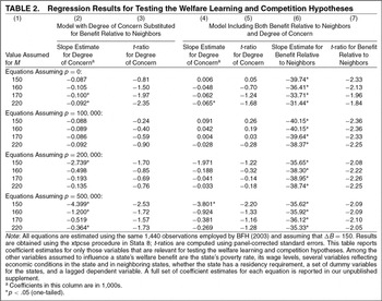
To test the welfare competition hypothesis, we substitute for benefit relative to neighbors each of our 48 measures (relying on varying assumptions about the values of M, Δ B, and p) of the degree of concern by state officials about welfare migration. Because findings tend to be stable across the three values of Δ B ($100, $150, and $200), to save space, we report results only for models assumingΔ B=150.
The learning hypothesis receives empirical support. The estimated coefficient for benefit relative to neighbors is −39.52, a value statistically significant in the predicted direction at the .05 level (t=−2.30). This estimate implies that when a state's AFDC benefit relative to its neighbors increases from its fifth percentile value in the sample to its ninety-fifth percentile value (and all other independent variables in the model are held constant), the state is expected to reduce its monthly benefit for a family of four by about 34 (1995) dollars in the first year.12
The mean monthly AFDC benefit for a family of four across state-years in our sample is $660. Because there is a lagged dependent variable in the model, estimated coefficients for independent variables reflect immediate impacts, the total effects of which are distributed over time (Gujarati 1995, 599–600).
BFH's (2003) benefit relative to neighbors variable is based on a weighted average (by population) of the benefit level in neighboring states. This is appropriate for a welfare learning model that assumes that states pay more attention to the benefit level in a populous neighbor than in a state of smaller size. A different learning model would assume that states are equally attentive to each of their neighbors, viewing all their neighbors as reasonable “benchmarks” regardless of their size. To test this alternative learning model, we estimate an equation that employs a measure of benefit relative to neighbors based on the unweighted average of benefits in contiguous states. For this equation too, the coefficient estimate for benefit relative to neighbors is negative and statistically significant.
The results regarding the welfare competition hypothesis—in which concern about welfare migration is substituted for benefit relative to neighbors—are presented in columns 2 and 3 of Table 2. The coefficient estimates for degree of concern are uniformly negative as predicted, and 6 of the 12 are statistically significant at the .05 level. Yet, even the coefficient estimates that are statistically significant do not indicate that states respond to increases in concern about welfare migration with substantial decreases in welfare benefits. We calculate the predicted reduction in welfare benefits resulting from a change in the degree of concern from its fifth percentile value in the sample to its ninety-fifth, when all other independent variables are held constant, based on each of the six regressions in which the coefficient estimate for degree of concern is statistically significant. The predicted response ranges from a decrease of about four (1995) dollars in the monthly AFDC benefit for a family of four in the first year to a decrease of around $13—with the average response being slightly more than $7. This average decrease of $7 is about one fifth the size of the predicted $34 decrease resulting from an increase in benefit relative to neighbors from the fifth percentile to the ninety-fifth. Therefore, in the case of welfare, our empirical analysis offers stronger evidence for the learning hypothesis than the competition hypothesis.
However, a more compelling test of the two hypotheses can be accomplished by including both degree of concern and benefit relative to neighbors in the same model. Column 6 of Table 2 shows coefficient estimates for benefit relative to neighbors in such models. When degree of concern is controlled, all 16 slope coefficient estimates for benefit relative to neighbors attain statistical significance, and the average change in their magnitudes is a decline of just 6%. In contrast, of the six models in which the estimated effect of degree of concern is statistically significant when benefit relative to neighbors is not in the model, only two show degree of concern still significant after benefit relative to neighbors is added (see column 4); and across the six models, the coefficient estimate for degree of concern decreases in magnitude, on average, by 26%. Thus, there is little empirical evidence suggesting that states compete vigorously over benefit levels, adjusting benefits substantially in response to a concern about the potential migration of the poor. However, our data analysis strongly supports the policy-learning hypothesis that policymakers view welfare benefits in neighboring states as benchmarks for determining a reasonable benefit level and adjust their benefit levels accordingly.
In 1996, Congress eliminated AFDC and replaced it with Temporary Assistance for Needy Families (TANF). We see no reason for expecting state officials to be more or less prone to search for benchmarks for their welfare benefits under TANF than under AFDC, and thus no reason to believe that welfare policy learning has changed with the introduction of TANF. However, the incentives for state officials to compete over welfare benefits have changed significantly since the adoption of TANF. Although states set their own benefit levels under AFDC, and they continue to do so under TANF, the categorical grant for AFDC made it so that the federal government paid for at least half of every dollar of benefit provided to each AFDC recipient. In contrast, the block grant for TANF makes it so that the marginal cost of an increase in welfare benefits is borne completely by the states, and the marginal benefit of a benefit decrease accrues exclusively to the states. Thus, one might reasonably expect that the incentive for state officials to compete over welfare benefits has increased. On the other hand, under the tight federal controls of AFDC, any competition among states was largely confined to the benefit levels set. TANF affords states much greater autonomy over a range of provisions of their welfare programs, including the discretion to set time limits, impose personal responsibility requirements and create work incentives. Because under TANF, states can discourage welfare migration by adjusting other provisions of their programs, this might lessen the motivation to undercut other states' benefits. In effect, under TANF, the focus of competition may have shifted from benefit levels to other dimensions. Thus, it is not obvious whether our evidence of a lack of vigorous benefit competition would extend to the contemporary welfare environment. On this issue, we must await empirical tests based on data from the TANF era.
CONCLUSION
The diffusion of public policy across the American states detected in a wide variety of policy areas has been attributed to two fundamentally different processes: policy learning and economic competition. Most empirical analyses of interstate influence have used a simple specification that assumes that states are influenced equally by all their neighbors, and uninfluenced by states that are not contiguous. Such a specification is reasonable for some versions of a learning model, but is generally inappropriate for testing a competition model because when a policy diffuses due to competition, states should be influenced by other states to varying degrees depending on the size and location of specific populations within the states. We have shown how geographic information systems can be used to test competition models of policy diffusion.
Although previous studies have claimed that the diffusion of both lottery adoptions and welfare benefit levels is due to interstate competition, using GIS we find evidence of competition only in the case of the lottery. We cannot say definitively why this is so, but we can speculate. Both our lottery and welfare models assume that for many individuals, the propensity to engage in the behavior of concern is appreciably greater than zero. In the case of the lottery, there is little doubt that this assumption is true. It is clear not only that state officials perceive that people living near a state border will cross it to play the lottery, but that many people do travel to other states for this purpose (Fink and Rork 2003, Mikesell 1987). It is far less certain that a significant number of poor persons migrate for better welfare benefits. Critics have challenged the hypothesis that the poor migrate for more generous public assistance on a variety of grounds—arguing that it ignores the substantial costs of relocation (which are especially burdensome on individuals with few economic resources), and assumes unreasonably that the poor are more concerned with welfare benefits than with private economic opportunities (Schram, Nitz, and Krueger 1998). Indeed, the most common result of individual-level research is that there is relatively little such migration (e.g., Allard and Danziger 2000; for a review of this literature, see Allard 1998).13
Even Bailey (2005, 134), who claims that this research underestimates the amount of welfare migration, concludes that although “welfare benefits exert a nontrivial effect on state residential choice,” the poor do not move in large numbers for greater welfare benefits.
Although it is possible that state officials believe that substantial welfare migration occurs even if it does not, and set policy based on this belief, our empirical evidence is consistent with an argument that policymakers do, in fact, recognize that large-scale migration of the poor is not a realistic concern.
The GIS techniques we have employed to study state policymaking would also be useful to political scientists and policy analysts studying competition among other jurisdictions. Indeed, there is a large literature on competition among local governments (e.g., Peterson 1981, Schneider 1989). One application of our approach would be a study of whether municipalities compete to have low sales tax rates due to a concern about residents going to a nearby jurisdiction to shop. An international relations application might assess whether immigration policies diffuse among European Union (EU) nations due to concern about individuals in nearby less developed non-EU countries immigrating for better economic opportunities. With GIS, the possibilities for careful empirical tests of models of spatial influence are vast.
An earlier version of this paper was presented at the 2004 Meeting of the Midwest Political Science Association, Chicago, IL. We thank Charles Barrilleaux, Frances Berry, Justin Esarey, Richard Fording, David Kimball, David Lowery, Chris Mooney, Chris Reenock, Evan Ringquist, John Scholz, and Craig Volden for their comments on earlier drafts. To save space, some tables of statistical results are excluded; all such tables are in an unpublished supplement available at the ICPSR Publication-Related Archive along with a replication data set.






Comments
No Comments have been published for this article.