Introduction
Accurate estimations of atmospheric longwave irradiance (LWI) at the surface are important in determining the radiation budget wherever direct measurements are not available. With the aim of providing a longwave radiation climatology that would be useful for validating Global Circulation Model (GCM) computations, King (Reference King1996) investigated seasonal and spatial variations of LWI in Antarctica, making use of data supplied by four stations: two representative of the coastal climatological regime (Syowa & Neumayer), one of the Antarctic region characterized by the strong katabatic winds regime (Mizuho), and one of the Antarctic Plateau (South Pole). The study was not able to discern between clear and cloudy-sky conditions because monthly means were used, thus limiting the possibility to investigate the particular characteristics of radiative processes in the Antarctic atmosphere under clear or cloudy-sky conditions separately.
In a cloud-free atmosphere assumed to behave as a grey body, LWI is a function of the vertical profiles of temperature and greenhouse gas concentrations. Since measured vertical profiles of these parameters are not always available for accurate radiative transfer calculations, LWI is usually parameterized in terms of an appropriate temperature, making use of the Stefan-Boltzmann emission law for a grey body:
 $$ LWI\, = \,{\epsilon}\sigma {{T}^4}, \eqno\rm$$
where σ is the Stefan-Boltzmann constant and T is the reference temperature, which requires the definition of an effective atmospheric emissivity ε. Many empirical and physically based formulations have been developed since the pioneering works of Ångström (Reference Ångström1918) and Brundt (Reference Brundt1932) to describe the relationships between effective clear sky emissivity ε and surface observations of temperature and water vapour content (Swinbank Reference Swinbank1963, Idso & Jackson Reference Idso and Jackson1969, Ohmura Reference Ohmura1982, Zillman Reference Zillman1972, Guest Reference Guest1998). The success of such methods in representing LWI features strongly depends on the site climatology.
In the presence of a variable thermal gradient in the boundary layer, a parameterization based on ground-level measurements is likely to be erroneous. Gröbner et al. (Reference Gröbner, Wacker, Vuilleumier and Kämpfer2009) pointed out that parameterizations of clear sky LWI can be considerably improved by making use of an effective atmospheric boundary layer temperature instead of surface temperature. Moreover, using the ground temperature Tg in Eq. (1) typically produces a daily oscillation of modelled LWI, according to the variations of Tg, which is not usually observed during measurements performed for clear sky conditions, for example at Dome C. Hence, the applicability of previous parameterizations to the extremely cold and dry conditions of the Antarctic Plateau is not obvious due to the presence of a significant and persistent temperature inversion throughout the year except for a short period during the summer (Hudson & Brandt Reference Hudson and Brandt2005, Genthon et al. Reference Genthon, Town, Six, Favier, Argentini and Pellegrini2010). The strong and persistent inversion is mainly due to the higher emissivity of the snow surface εs, with value very close to one (Warren Reference Warren1982), with respect to the emissivity of the atmosphere εa for clear sky conditions. Considering that during winter the effect of solar radiation is absent, and that typically only 15% of the energy balance at the surface involves latent heat and sensible heat fluxes, Hudson & Brandt (Reference Hudson and Brandt2005) set the relation  $$--><$>{{{\epsilon}}_a}{{T}_a}^{4} \, \approx \,0.85{{{\epsilon}}_s}{{T}_s}^{4} $$$
between air temperature Ta and the temperature of the snow surface Ts. For a typical value for the εa ~ 0.6, this equation implies that Ta > Ts.
Accurate measurements of the infrared radiation in polar regions became routinely available with the establishment of the first Baseline Surface Radiation Network (BSRN) sites in the 1990s. Dome C, located on the East Antarctic plateau (75.1°S, 123.3°E, 3233 m above mean sea level), joined this community in 2006 (Lanconelli et al. Reference Lanconelli, Busetto, Dutton, König-Langlo, Maturilli, Sieger, Vitale and Yamanouchi2011) when continuous measurements of LWI started to be performed routinely at the Italian-French station, Concordia (http://www.concordiabase.eu).
In this study, the LWI measurements collected in the period from January 2006–December 2008 were investigated to determine a suitable parameterization of the clear sky LWI for Dome C. Besides radiation measurements, the one-minute resolved standard meteorological parameters, available from the automatic weather station (AWS) operating at Concordia, and radio sounding measurements, performed every day at 20h00 local time (LT) (12h00 UTC), were used.
Methodology
In most existing parameterizations, atmospheric emissivity ε is expressed as a function of the surface temperature Tg and/or water vapour partial pressure e (Pirazzini et al. Reference Pirazzini, Nardino, Orsini, Calzolari, Georgadis and Levizzani2000, Duarte et al. Reference Duarte, Dias and Maggiotto2006). Carrying out accurate measurements of the air relative humidity (RH) in extremely cold regions with standard instruments is difficult. Therefore, considering the extremely dry air-conditions of Dome C (Tomasi et al. Reference Tomasi, Petkov, Stone, Benedetti, Vitale, Lupi, Mazzola, Lanconelli, Herber and von Hoyningen-Huene2010), we decided to parameterize ε in terms of temperature only. In such a way the estimation of clear sky LWI can be expressed in terms of the following equation:
 $$ LWI\: = \:{\epsilon}(T)\sigma {{T}^4}, \eqno\rm$$
where T is usually assumed to be the air temperature at the surface Tg, also called screen temperature. However, previous studies showed that in the presence of a surface temperature inversion, the temperature at the top of the inversion layer (hereafter Tm, i.e. the maximum temperature) appears more suitable for reproducing LWI clear sky measurements (Yamanouchi & Kawaguchi Reference Yamanouchi and Kawaguchi1984, King Reference King1996). Considering that Tm is expected to be more stable during the day (Hudson & Brandt Reference Hudson and Brandt2005, Aristidi et al. Reference Aristidi, Agabi, Fossat, Vernirn, Travouillon, Lawrence, Meyer, Storey, Halter, Roth and Walden2005), the modelled LWI should appear more realistic, being unaffected by the surface temperature oscillations related to the solar radiation cycle.
Wind speed and direction could also affect LWI, because of snow drifting or advection and katabatic flows. At Dome C and South Pole the mean wind speed is much lower than the limit of 13 ms-1, below which drifting snow does not influence the downward longwave flux (Yamanouchi & Kawaguchi 1994), and the region of Dome C is not influenced by katabatic winds. Due to the distance from the coasts (about 1200 km) and the site elevation (3300 m), together with the presence of the polar vortex, the advection from the ocean cannot be easily correlated with wind speed (Udisti et al. Reference Udisti, Dayan, Becagli, Busetto, Frosini, Legrand, Luccarelli, Preunkert, Severi, Traversi and Vitale2012). For these reasons, we do not use wind data in our LWI parameterization.
Longwave measurements and cloud screening
Downwelling longwave irradiance is continuously measured at Dome C using a pyrgeometer manufactured by Kipp & Zonen (model CG4) calibrated against the World Infrared Standard Group (WISG) hosted at the Physikalisch-Meteorologisches Observatorium Davos/World Radiation Centre (PMOD/WRC), Switzerland. All the measurements are subjected to detailed automatic and manual quality-check procedures, in accordance with BSRN recommendations (Long & Dutton Reference Long and Dutton2002).
The method proposed by Town et al. (Reference Town, Walden and Warren2007) was used to remove cloud contaminated data. This method (hereafter referred to as scatter plot method) is based on the analysis of the scatter plot of LWI standard deviation calculated over a 20-minute time interval vs LWI itself centred on the same interval. Its application requires the determination of a suitable clear sky LWI limit and associated standard deviation thresholds. For the latter, a value of 0.8 W m-2 was chosen according to Town et al. (Reference Town, Walden and Warren2007), while the monthly longwave thresholds were determined on the basis of the Santa Barbara Discrete Ordinate Radiative Transfer (DISORT) Atmospheric Radiative Transfer (SBDART) code (Richiazzi et al. Reference Ricchiazzi, Shiren, Gautier and Sowle1998) calculations.
Temperature, pressure and water vapour density monthly mean profiles under clear sky conditions, as defined by Tomasi et al. (Reference Tomasi, Petkov, Stone, Benedetti, Vitale, Lupi, Mazzola, Lanconelli, Herber and von Hoyningen-Huene2010), were used in SBDART calculations. Due to the lack of ozone profile data over Dome C, the standard sub-Arctic winter and summer ozone density profiles were used. The negligible influence of ozone density profiles in evaluating LWI using SBDART does not affect the results given by the scatter plot method, and this approximation does not significantly affect evaluations presented in this paper.
Values of these thresholds from January–December are given in Table I for Dome C. They assume a minimum of 68 W m-2 in September, and a maximum of 115 W m-2 in December.
Monthly values of the longwave irradiance (LWI) thresholds used to identify the clear sky situations making use of the scatter plot method, monthly averages of LWI and standard deviations σLWI, fractions of clear sky periods per month, and number of minutes of LWI valid measurements available in the dataset. SBDART = Santa Barbara Discrete Ordinate Radiative Transfer (DISORT) Atmospheric Radiative Transfer.

The left panels of Fig. 1 shows the scatter plots for January (Fig. 1a) and July (Fig. 1c), which represent typical conditions occurring in summer and winter, respectively. Following Town et al. (Reference Town, Walden and Warren2007), the bottom-left part of each scatter diagram (quadrant I) is assumed to pertain to clear sky conditions while quadrant IV is assumed to represent overcast conditions and quadrants II and III represent partially cloudy conditions. The right panels of Fig. 1 report the corresponding scatter plot of LWI vs Tg and a series of grey-body curves with emissivities varying between 1.0 (black body) and 0.4. Points with the lower LWI standard deviation are confined between the 0.4–0.6 emissivity range during January (Fig. 1b), while they cover mainly the 0.5–0.7 emissivity range during July (Fig. 1d).
a. & c. Scatter plots of longwave irradiance (LWI) vs its standard deviation calculated over a 20-min temporal window for the overall January (a.), and July (c.) Dome C data. The thresholds (black dashed lines) for LWI have been calculated by Santa Barbara Discrete Ordinate Radiative Transfer (DISORT) Atmospheric Radiative Transfer (SBDART) using mean monthly profiles of temperature and absolute humidity, while the threshold for standard deviation has been chosen to be 0.8. Clear sky cases are expected to join the quadrant I. b. & d. The same LWI values plotted vs the ground temperature Tg. Curves represent the black body emissions with emissivity 1, 0.8, 0.6 and 0.4 from top to bottom respectively.

As the LWI is expected to be higher in the presence of clouds than in clear skies, for the same near-surface temperature, the upper limit of such a dataset can be considered to be representative of overcast conditions, while the lower limit pertains to clear skies, in accordance with the scatter plot method shown in the left part of Fig. 1. On the other hand, cloudy-sky cases, for which effective emissivity values greater than unity were observed, correspond to strong temperature inversions in conjunction with the presence of low-level stratus clouds, as shown by König-Langlo & Augstein (Reference König-Langlo and Augstein1994).
Using this method, the complete Dome C dataset was evaluated. The frequencies of clear sky varied from 35% in May, the cloudiest period, to 70% in February. Table I shows the monthly mean and standard deviations σ LWI of LWI.
Figure 2 shows the time series of LWI, Tg and the effective emissivity εg calculated for inversion of Eq. (2) with respect to Tg. Longwave irradiance varies in the range 50–200 W m-2, showing seasonal behaviour in phase with the ground temperature Tg, with minima during colder seasons, and in general related to clear sky conditions identified by the black points. The upper LWI limit decreases by about 100 W m-2 considering only clear sky cases (black points). The strong cooling of the air at the ground level, expected to be more frequent during clear sky conditions, can be better observed during winter when the clear sky cases occupy the lower limit of the curve in the central graph of Fig. 2. By contrast, during summer, when the surface warms due to the interaction with solar radiation, clear sky cases span the entire temperature interval. The effective emissivity calculated from the previous time series confirms the results observed in Fig. 1b & d for January and July, giving a well defined overview of the range spanned in all-sky (0.4–1.1) and clear sky (0.4–0.7) situations. For clear sky cases the seasonal oscillation is counter-phased to LWI and Tg, indicating that the surface temperature is not representative of the overall thermal conditions of the boundary layer. In fact, the extremely low temperatures reached during winter due to a radiative cooling of the surface are not matched by a corresponding decrease of the LWI. Therefore, if Tg is used to describe LWI through Eq. (1), a variable effective emissivity is required.
Dome C data. Upper part: time series of the longwave irradiance (LWI). Middle part: time series of ground temperature Tg. Lower part: time series of the equivalent black-body emissivity  $$--><$>{{{\epsilon}}_{\rm{g}}}\, = \,{\rm{LWI}}{{\sigma }^{{\rm{ {\hbox-} 1}}}} {{{\rm{T}}}_{\rm{g}}}^{{{\rm{ {\hbox-} 4}}}} {}$$$
. Grey lines represent all-sky conditions, and black dots represent clear sky cases detected with the scatter plot method described in the text.
Radiosonde data and surface inversions
Radiosondes are routinely launched at Dome C every day at 12h00 UTC (20h00 LT), employing Vaisala radiosondes, model RS92. The measurements performed from January 2006–December 2008 were examined in order to study the behaviour of the thermal inversion structure.
Each radiosonde measurement provides values of the thermodynamic parameters (pressure, air temperature, relative humidity) along with other supplementary data such as wind speed and direction, up to an altitude of about 20 km with a resolution of about 8–12 m in altitude. Radiosonde temperature data can be affected by two kinds of errors, the first arising mainly from solar heating and heat exchange between the radiosonde thermocap sensor and the surrounding air, the second due to the time lag of sensor response. The heat exchange errors were corrected following the standard procedure provided by Vaisala, according to Luers (Reference Luers1997), while the time lag error for RS92 radiosondes was negligible, and hence, no correction was made to the raw temperature data.
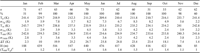
Using Dome C radiosonde data, we found that the maximum temperature in the lower troposphere during winter is reached at a height of about 400 m. During January and December the inversion is weak or is replaced by almost isothermal conditions. Moreover, Aristidi et al. (Reference Aristidi, Agabi, Fossat, Vernirn, Travouillon, Lawrence, Meyer, Storey, Halter, Roth and Walden2005) and Hudson & Brandt (Reference Hudson and Brandt2005, their fig. 22) highlighted the fact that the temperature inversion extends usually up to 150 m and temperature profile above 150 m is isothermal with height and stable (within c. 2 K) during summer days.
Ricaud et al. (Reference Ricaud, Genthon, Durand, Attié, Carminati, Canut, Vanacker, Moggio, Courcoux, Pellegrini and Rose2012) showed, based upon microwave radiometer measurements carried out at Dome C, that there is a weak diurnal variation of temperature ( $$\[--><$>\rDelta<$><!--$$
T) above 150 m. The effect of this variation on LWI in T is <1 W m-2, and so can be neglected.
Based on these observations, we have adopted T400 as a good approximation of Tm. A similar assumption was adopted by Yamanouchi & Kawaguchi (Reference Yamanouchi and Kawaguchi1984), who studied longwave emissions under surface inversions at Mizuho (Antarctica), utilizing the temperature measured at 300 m, the typical inversion level at that site.
Table II reports the values of some statistical parameters characterizing the temperature profiles, obtained on a monthly basis, using the Dome C radio soundings. For January and December the values were calculated only for the inversion cases. From February–November the temperature inversion is always present, while the frequency of inversion cases is smallest in December (50%) and January (60%). During these two months the inversion strength ΔT, defined as T400 - Tg, assumes minimum values, i.e. about 2 K on average, when the temperature inversion is frequently replaced by isothermal conditions. From March–October ΔT assumes values around 20 K or higher and is quite stable during the period. This atmospheric temporal stability is an important feature of the winter in the high Antarctic Plateau (Phillpot & Zillman Reference Phillpot and Zillman1970). The seasonal differences between winter and summer conditions are similar to those reported by Hudson & Brandt (Reference Hudson and Brandt2005) for South Pole. This behaviour is mainly due to the effect of the solar radiation on the snow surface, which causes convective activity due to surface heating (Argentini et al. Reference Argentini, Viola, Sempreviva and Petenko2005). Table II clearly shows that monthly averages of Tm and T400 are consistent within their standard deviations. These standard deviations are generally lower than that of Tg, except for January and December when the inversion is much weaker, indicating that the maximum temperature is more stable than the ground temperature throughout the year. Figure 3 shows the time series of T400 and Tg. The ground temperature varies seasonally by about 60°C from -80°C to -20°C, while T400 varies by only 30°C, from -45°C in winter to -15°C in summer.
Values of radio sounding statistical parameters evaluated at Dome C in the three-year period from 1 January 2006–31 December 2008: first row gives the number of radiosonde launches, second row the percentage of temperature profiles with inversion in the ground layer. Parameters Tg, σTg, Tm, σTm, T400 and σT400 are the monthly means and standard deviations of ground, inversion and 400 m temperature, respectively; ΔT is the difference Tg - Tm, H is the mean value of the inversion layer height. All values are valid for the time of the radiosonde (20h00 local time), and, for January and December, they have been calculated for the inversion cases only.
Time series of ground temperature Tg (circles) and temperature at 400 m T400 (triangles) measured by the radiosondes at 20h00 local time. Vertical grey bars represent the daily surface temperature variations measured by the automatic weather station. Red and blue lines represent running averages of T400 and Tg calculated over a box of 30 days, respectively.
Figure 4 shows the plot of T400 vs Tg, as obtained from both all-sky and clear sky radiosonde data. Clear sky conditions are selected using the results of the scatter plot method, obtained within a period of ± 1h around the nominal launch time of 20h00 LT. Since the scatter plot method flags cloudy/clear each minute, the radiosonde is considered to be performed for clear sky conditions if at least 90% of the flight period was detected as clear. Figure 4 shows that the best fit regression line, calculated only for inversion cases, does not change appreciably between clear and cloudy contaminated radiosonde measurements. This confirms that the presence of clouds of a low optical depth on the Antarctic Plateau does not significantly affect the establishment of a thermal inversion in the boundary layer caused by surface cooling. The linear best fit for clear sky cases is given by:
 $$ {{T}_{400}}\: = \:168\: + \:0.31{{T}_g}, \eqno\rm$$
with temperatures expressed in Kelvin and a regression coefficient of r 2 = 0.86.
Scatter plot of temperature at 400 m T400 vs ground temperature Tg for all radio sounding performed at 20h00 local time available for the entire period (2006–08) at Dome C. Grey points refer to all sky conditions and cyan points to clear sky. Reported linear fits have been evaluated only for thermal inversion cases. Filled line refers to Dome C clear sky points, dashed line to Dome C all-sky.
In terms of inversion strength ΔT defined as the difference between T400 and Tg, Eq. (3) can be rewritten as  $$--><$>\rDelta T\, = \,168\,{\rm{ - }}\,0.69{{T}_g} $$$
. Here, the slope coefficient we found is about 10% higher than that indicated by Connolley (Reference Connolley1996) for the interior of the continent, using monthly averages of Tm and Tg measured at Vostok and South Pole.
Figures 3 & 4 also show that, in the higher temperature range, some values of T400 are very close to Tg, indicating cases without inversion. For these conditions, observed only during January and December as shown in Table II, the mean ground temperature value, 246.1 K in January and 245.8 K in December, is comparable to the mean value of the measured T400, 246.2 K and 245.0 K, respectively for January and December, highlighting an isothermal-like behaviour of the lower troposphere in the absence of an inversion. Nearly isothermal conditions in the lowest kilometre of the troposphere were also reported by Hudson & Brandt (Reference Hudson and Brandt2005) during summer months at South Pole. Applying Eq. (3) to these cases leads to mean value of the computed T400 of 244.3 K in January and 244.2 K in December, both lower than observed. Hence, without thermal-based inversion conditions, the proxy temperature T400 is considered equal to the ground temperature and not calculated using Eq. (3). On average, it is possible to define a temperature threshold of about 244 K, above which inversion never occurs, given by the intersection of Eq. (3) with the condition T400 = Tg.
Considering both the cases of inversion and its absence, the relationship providing T400 as a function of Tg becomes:
 $$ {{T}_{400}}\, = \,f({{T}_g})\, = \,\left\{ \matrix{ 168 + 0.31{{T}_g} \quad {{T}_g}\,\leq \,244K \\ {{T}_{g}}\; \; \; \; \ \ \ \quad \qquad \; \;{{T}_g}\, \gt \,244K\hfill<! \\ >\right. \eqno\rm$$
Ground temperature diurnal cycle
Equation (4) is valid only for the time interval during which each radio sounding is performed at Concordia Station, i.e. at 12h00 UTC (20h00 LT). The use of Eq. (4) at a different time t of the day should induce a certain inaccuracy in evaluating T400(t), because of the strong variations of Tg(t) throughout a summer day, from a morning minimum to a maximum in the early afternoon, closely related to the solar zenith angle cycle. In fact, Eq. (4) attributes approximately one third of the Tg daily variation amplitude to T400, in case of inversion while, without inversion, T400 and Tg assume the same daily variation amplitude. As pointed out in the previous section, Hudson & Brandt (Reference Hudson and Brandt2005), Aristidi et al. (Reference Aristidi, Agabi, Fossat, Vernirn, Travouillon, Lawrence, Meyer, Storey, Halter, Roth and Walden2005) and Ricaud et al. (Reference Ricaud, Genthon, Durand, Attié, Carminati, Canut, Vanacker, Moggio, Courcoux, Pellegrini and Rose2012) showed that diurnal variation is negligible at levels over 150 m. Hence, T400(t) during the day can be considered equal to the temperature at 400 m recorded by the radiosonde at 20h00 LT, i.e.
 $$ {{T}_{400}}(t)\: \approx \:T_{{400}}^{{RDS}} \: \approx \:f(T_{g}^{{RDS}} ), \eqno\rm$$
where the form of function f has been given in Eq. (4) and  $$--><$>{{T}_g}^{{\!\!RDS}} $$$
is the ground level temperature measured during radiosonde flight.
There is also a variability in the temperature that is not linked to the incoming solar radiation, especially during winter, which is instead due to the approach of cyclones to Antarctica from lower latitudes (Enomoto et al. Reference Enomoto, Motoyama, Shiraiwa, Saito, Kameda, Furukawa, Takahashi, Kodama and Watanabe1998) and to interplanetary magnetic field variation (Troschiev et al. 2008). In all cases such temperature variations are associated with a cloud layer formation at heights of 6–8 km (Troshichev et al. Reference Troshichev, Vovk and Egorova2008, page 1297), and they were not considered here since the parameterization given in this paper is for the clear sky emissivity.
Figure 5 reports the monthly mean Tg daily evolutions. In the left part, the months characterized by presence of sun are reported, while in the right part, data are plotted for months without sunshine relevant effects. The Tg diurnal variation can be referred, following a method similar to that of Dürr & Philipona (Reference Dürr and Philipona2004), to the daily average ground temperature  $$--><$>\overline{{{{T}_g}}} $$$
, through a simple sinusoidal form with a 24-hour period, appropriate amplitude Ad, angular frequency
 $$--><$>{{\omega }_d}\, = \,{\rm{2}}\pi \,/\,{\rm{24}} $$$
and a phase ϕd, as follows:
 $$ {{T}_g}(t)\, = \,\overline{{{{T}_g}}} \, + \,{{A}_d}\;\cos \left( {{{\omega }_d}t\: + \:{{\varphi }_d}} \right), \eqno\rm$$
where the time t is expressed in LT hours.
Left: Dome C data. Monthly mean daily behaviour of the ground temperature Tg for months from September–April. Right: same values plotted for polar night months (June and July) and last/first sunrise month (May and August). The vertical dashed lines correspond to the radiosonde launch time (20h00 local time), the filled lines reproduce Eq. (6) with phase ϕd = 3π/4 and amplitude Ad = 6 K from November–February, 4 K for March and October, 2 K for April and September and set to zero for the months reported in the right part of the figure.
As shown in Fig. 5, amplitude Ad can be assumed equal to 6 K for the summer months November–February, 4 K for March and October, 2 K for transitional months April and September (left part of Fig. 5), and zero for the other winter months (right part of Fig. 5) when there is no sun and, hence, daily variation is absent. The phase ϕd was evaluated to be well represented by 3/4π on average, a value that shifts the cosine function nine hours early. This phase value provides good fits in January, February, November and December, when the diurnal cycle is more evident. The assumption of the same value over the whole year does not significantly affect the results because the amplitude becomes gradually lower moving towards winter.
From Eq. (6), the temperature Tg RDS at radiosonde launching time (20h00 LT), can be evaluated in terms of the following equation:
 $$ T_{g}^{{RDS}} \: = \:{{T}_g}(t)\, {\rm{ - }}\, {{A}_d}\left[ {\cos \left( {{{\omega }_d}t\: + \:{{\phi }_d}} \right)\:{\rm{ - }}\:\cos \left( {{{\omega }_d}{{t}^{RDS}} \: + \:{{\phi }_d}} \right)} \right] .\eqno\rm$$
Combining Eqs (5) & (7), T400 for clear sky conditions can be evaluated during the whole day using the following equation:
 $$ {{T}_{400}}(t)\, = \,f\left( {{{T}_g}(t)\,{\rm{ - }}\,{{A}_d}\left[ {\cos \left( {{{\omega }_d}t\: + \:{{\phi }_d}} \right)\,{\rm{ - }}\,\cos \left( {{{\omega }_d}{{t}^{RDS}} \: + \:{{\phi }_d}} \right)} \right]} \right), \eqno\rm$$
where the function f has been defined in Eq. (4).
Parameterization of clear sky emissivity
As previously discussed, the clear sky longwave flux and emissivity can be expressed in terms of appropriate temperature values, which should be chosen to realistically represent the thermal conditions of the boundary layer. Usually the ground temperature Tg is adopted. However, we have used T400, taking into account that T400 and Tg are related by Eq. (8).
Effective emissivity was evaluated by inverting Eq. (2), using hourly averages of LWI corresponding to radiosonde launching, and both Tg and T400 as reference temperatures. The left panels of Fig. 6 show the emissivity calculated with respect to the ground temperature (εg = LWI/σTg 4) vs Tg itself (upper) and vs precipitable water content w as obtained from radiosonde (lower), while the right panels show emissivity calculated using T400 (εm = LWI/σT400 4) vs T400 (upper) and w (lower). It is evident that effective emissivity is better correlated with temperature and w, when it is calculated with respect to T400 rather than Tg. Furthermore, εg results to decrease with Tg showing an unrealistic behaviour. In fact, as temperature increases the saturation vapour pressure increases and hence, emissivity is expected to increase.
Left: clear sky effective emissivity,  $$--><$>{{{\epsilon}}_{\rm{g}}}\, = \,{\rm{LWI}}{{\sigma }^{{\rm{ {\hbox-} 1}}}} {{{\rm{T}}}_{\rm{g}}}^{{{\rm{ {\hbox-} 4}}}} {} $$$
plotted vs Tg (upper part) and vs vertical water content w obtained from Dome C radiosondes (lower part). Right: clear sky effective emissivity,
 $$--><$>{{{\epsilon}}_{\rm{m}}}\, = \,{\rm{LWI}}{{\sigma }^{{\rm{ {\hbox-} 1}}}} {\rm{T}}_{{400}}^{{{\rm{ - }}4}} $$$
, plotted vs T400 (upper part) and w (lower part). Regression lines for εg(Tg), εm(T400) and εm(w) are reported. In the lower part points colour represent Tg (left) and T400 (right), while in the upper plots, the colour scale represents w. The isolines of longwave irradiance (LWI) are also reported in steps of 20 W m-2 in the upper part of the figure.
The regression line reported in the right part of Fig. 6, relating to T400, is
 $$ {{{\epsilon}}_m}\, = \,{\rm{ - }}1.41\: + \:0.0077{{T}_{400}}, \eqno\rm$$
which shows an increase in the emissivity with increasing reference temperature, as expected. Assuming a square root dependence of the emissivity on water vapour content, experimental data can be approximated by  $$--><$>{{{\epsilon}}_m}\, = \,0.24\, + \,0.32\sqrt w $$$
(w in g cm-2) with a regression coefficient r 2 = 0.8. By contrast, εg does not show an evident correlation with w.
These considerations confirm that, in the presence of a temperature inversion, the use of T400 is more appropriate than Tg, in describing the emission properties of the atmosphere. In order to evaluate the emissivity as a function of ground based measurements, T400 was preferred to w since it is easily related with Tg and because measuring RH using standard procedures is quite problematic in such cold and dry environments. Furthermore, there is a linear relationship between w and T400 with a correlation coefficient r 2 = 0.8 (not shown), indicating that T400 itself contains information on the precipitable water content, since the saturation vapour pressure increases with air temperature.
Since both LWI and T400 show little diurnal variability on clear sky days, Eq. (9) can be assumed to be valid for the whole day.
Using Eqs (8) & (9), we compare the modelled emissivity with field measurements. The upper panel of Fig. 7 shows the time variability of the modelled and measured values of εm, and the lower panel shows their difference. Figure 7 highlights the existence of an annual cycle in the difference between modelled and measured values, presumably due to the variation of water vapour content, inversion strength, and other effects neglected in Eq. (9). In order to take this feature into account, the following time-dependent sinusoidal correction for the emissivity, with a one-year (365.25 days) period, was added:
 $$ \Delta {{{\epsilon}}_m}\, = \,{\epsilon}_{m}^{{MOD}} \,{\rm{ - }}\,{\epsilon}_{m}^{{MEA}} \, = \,{{A}_y}\cos \left( {{{\omega }_y}d\: + \:{{\varphi }_y}} \right), \eqno\rm$$
where d is the day of the year, Ay = 0.0261,  $$--><$>{{\omega }_y}\, = \,2\pi \,/\,365.25 $$$
and ϕy = 1.66. Such a phase value anticipates the maximum overestimation by 115 days with respect to the end of the year, placing it at the beginning of September. Similarly, the maximum underestimation was found in March, corresponding to a delay of a couple of months with respect to the warmest and moistest period of the year (December–January).
Upper part: emissivity εm modelled using Eq. (11) (MOD) and obtained from measurement as  $$--><$> LWI{{\sigma }^{{\rm{ - }}1}} T_{m}^{{{\rm{ - }}4}} $$$
(MEA) for the three-year Dome C dataset. Lower part: difference between modelled and measured emissivity with the corresponding best fit given in Eq. (10).
Inserting this time-dependent correction into Eq. (9), the following updated equation was obtained:
 $$ {{{\epsilon}}_m}\, = \,{\rm{ - }}1.41\, + \,0.0077{{T}_{400}}\,{\rm{ - }}\,{{A}_y}\cos \left( {{{\omega }_y}d\, + \,{{\varphi }_y}} \right) .\eqno\rm$$
Equation (11) gives the emissivity with respect to T400. Using Eq. (2), we can calculate LWI with  $$--><$>{{{\epsilon}}_m}\sigma T_{{400}}^{4} $$$
as long as
 $$--><$>{{{\epsilon}}_g}\sigma T_{g}^{4} $$$
, the latter expression being comparable with most parameterizations. The relation between two forms of emissivity,
 $$--><$>{{{\epsilon}}_g}\, = \,{{{\epsilon}}_m}{{\left( {{{T}_{400}}\,/\,{{T}_g}} \right)}^4} $$$
, allows to express LWI as a function of Tg:
 $$ LWI\: = \:{{{\epsilon}}_m}{{\left( {\frac{{{{T}_{400}}}}{{{{T}_g}}}} \right)}^4} \sigma T_{g}^{4}, \eqno\rm$$
Application of the methodology to South Pole data
South Pole, located on the Antarctic Plateau (89.98°S, 24.80°W, 2800 m above mean sea level), is a good site for testing the methodology presented in this paper for the calculation of LWI. South Pole has a similar atmospheric thermal structure to that observed at Dome C. Strong surface thermal inversions occur during winter, with mean strengths of 20–25 K, while the inversions are weaker or absent during summer (Hudson & Brandt Reference Hudson and Brandt2005).
The relationship between T400 and Tg is site-dependent, and needs to be reformulated for South Pole. First of all the daily cycle is not present, South Pole being situated at nearly 90°S, and Tg can be considered constant during the clear sky days. Therefore the relationship between T400 and Tg does not contain the time dependence term of Eq. (8).
Using radiosonde data obtained from the Wyoming University website (http://weather.uwyo.edu/upperair/sounding.html, accessed March 2010), a linear relationship between T400 and Tg, and the threshold temperature over which inversion should not occur were recalculated for South Pole, i.e.
 $$ {{T}_{400}}\, = \,f({{T}_g})\, = \,\left\{ {\begin{array}{*{20}c} {161\: + \:0.35{{T}_g} \quad{{T}_g}\,\leq \,248K} \hfill \\ {{{T}_g}\; \; \; \; \; \; \quad \qquad \;\;{{T}_g}\, \gt \,248K} \hfill \\\end{array}} \right., \eqno\rm$$
with regression coefficient r 2 = 0.82.
Comparing coefficients of Eqs (4) & (13), the South Pole linear best fit does not differ significantly from that evaluated for Dome C. This confirms the similarity of the thermal structure of the lower troposphere between the two plateau sites. Moreover, the precipitable water content values were found to be similar to those of Dome C, with values that vary from 0.1–0.8 mm at standard temperature and pressure (STP). Due to this similarity, the relation between εm and T400 can be assumed to be valid for both plateau sites.
Once T400 is evaluated using Eq. (13), it is possible to calculate the emissivity at South Pole, making use of Eq. (11), and hence the LWI from Eq. (12).
Results
The summer daily cycle
Figure 8 highlights the significant role of Eq. (8), which introduces the time-dependent cosine factor to correct for the daily cycle of Tg and maintains T400 constant during a day. The left panels of Fig. 8 show the scatter plot of the modelled vs measured LWI, while the right panels show the scatter plot of the estimates of LWI calculated without the cosine correction vs the field measurements. Data obtained for the overall three-years dataset recorded at night time (04h30 LT), day time (13h30 LT), and evening time (22h30 LT) are reported, as well as for those for the entire day. Without the time-dependent correction, the correlation between estimated and measured LWI varies according to the hours considered, providing better results for the warmer hours of the day (bias equal to 1.6 W m-2 and root mean square (RMS) equal to 6.3 W m-2 at 13h30 LT), and the worst results during the night hours (bias and RMS equal to -3.6 W m-2 and 7.2 W m-2, respectively at 04h30 LT). Using the cosine correction, the correlation does not vary much with time, with RMS values at different times of the day almost equal to 6.3 W m-2, while the bias reaches its minimum at 04h30 LT (-0.2 W m-2) and its maximum at 22h30 LT (-0.8 W m-2). Considering the overall dataset, RMS values for both estimates are similar: 6.2 W m-2 with cosine correction and 6.8 W m-2 without. However, the bias is lower for the cosine corrected estimation (-0.5 W m-2) than for the estimation without cosine correction (-1.1 W m-2). Thus, the introduction of Eq. (8) provides more accurate forecast of the time pattern of LWI during a sunny day.
Scatter plot of hourly averaged longwave irradiance (LWI) modelled using Eq. (12) and measured LWI for the whole three-year Dome C dataset at different local times. Left: Calculation of LWI with the time dependency of ground temperature of Eq. (8). Right: modelled LWI are calculated without the cosine correction. In all the plots the filled line represents the equation y = x and the dotted line the linear correlation. Bias, evaluated as the difference between modelled and measured values, and the root mean square (RMS) value, are also reported for each scatter plot.
As shown by Guest (Reference Guest1998) and Pirazzini et al. (Reference Pirazzini, Nardino, Orsini, Calzolari, Georgadis and Levizzani2000), various parametric models have been proposed in the literature for clear sky effective emissivity, based on the analytical forms listed in Table III. All the formulations reflect the summer daily cycle of Tg on LWI. The parameterization given in Eq. (11) depending on T400, does not show any daily cycle in agreement with measured LWI, because of the introduction of the cosine correction in the relation between Tg and Tm.
Description of the models of εeff used as concurrent for testing the parameterization developed in this study, including regions in which they were parameterized and air temperature range, when available.

The upper panels of Fig. 9 show the time patterns for a summer (January) and a winter (September) period, characterized by the sun's presence, of the following quantities: i) measured LWI; ii) LWI calculated using Eq. (12), where T400 is calculated with cosine correction, Eq. (8); iii) LWI calculated using Eq. (12), where T400 is calculated without cosine correction, Eq. (4); and iv) LWI calculated using the Swinbank (Reference Swinbank1963) formula.
Dome C data. Upper part: time patterns of measured and calculated longwave irradiance (LWI) using Eq. (12), with (Eq. (8)), and without (Eq. (4)) the daily cosine correction of T400. Longwave irradiance estimated with Swinbank parametric equation (Swi) is also reported. Lower part: measured value of Tg, T400 calculated using Eq. (8) and T400 calculated using Eq. (4). Blue points refer to the T400 measured by radiosonde. Left: summer period of December 2006. Right: same as before but for a colder winter period (September 2008).
In the lower panels of Fig. 9 the values of T400, calculated using Eqs (8) & (4), and of Tg are plotted for the same periods.
The LWI calculated using the Swinbank (Reference Swinbank1963) formula shows, especially during summer, a daily variation of about 25 W m-2 following the ground temperature variation, leading to an error that could be as high as 20 W m-2. The LWI calculated with the parameterization of Eq. (12) without the cosine correction also shows a daily variation, but with a smaller amplitude of about 15 W m-2, being related to the variation of T400 estimated with Eq. (4) and shown in the bottom part of Fig. 9. Taking the cosine correction of Eq. (8) into account in Eq. (12), the estimated values of LWI are not affected by the temperature daily cycle, and better approximate the measured values of LWI. These features are stronger in January, when the solar zenith angle variation is more pronounced, causing a more evident ground temperature daily cycle.
Comparison with other parameterizations
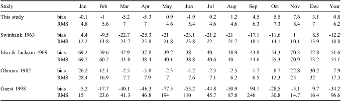
Figure 10 shows clear sky values of LWI and εg evaluated with the parameterizations given in Table III together with those obtained in this study - Eq. (12) - over the whole temperature range observed at Dome C. The dark grey points provide the three-hour running average values of LWI and εg vs Tg under clear sky conditions, while green points refer to their daily averages. Figure 10 clearly shows how the Idso & Jackson (Reference Idso and Jackson1969) parameterization leads to overestimated values of LWI over the whole temperature range. The curve obtained by Ohmura (Reference Ohmura1982) fits the LWI measurements better at low temperatures (Tg < 230 K) mainly observed during winter time, than at higher temperature, where it produces significantly overestimated values. Swinbank (Reference Swinbank1963) and Guest (Reference Guest1998) formulas give better results within the higher temperature range, but they significantly underestimate values at low temperatures.
Dome C data. Upper part: longwave irradiance (LWI) (left) and εg (right) plotted vs Tg. Grey and green points show the three-hour and daily averages of measured quantities, respectively. The parameterizations of Swinbank (Reference Swinbank1963), Idso & Jackson (Reference Idso and Jackson1969), Ohmura (Reference Ohmura1982) and Guest (Reference Guest1998), are reported along with Eq. (12) (left) and Eq. (11) (right). Lower part: evaluation of residual, calculated as difference between measured and parameterized values for the three-hour averaged data, for the LWI (left) and εg (right), with the best fit Gaussian curve in red.
These remarks are summarized in Table IV, where bias and RMS values, evaluated as difference between estimated and measured values of LWI, are reported for each month and for the whole three-year dataset using three-hour average data. Bias and RMS evaluated for Eq. (12) are almost constant throughout the year, emphasizing that the correlation does not depend much on the temperature range. Taking the complete dataset into consideration, the parameterizations developed in the present study provide the lowest bias and RMS values, indicating the best agreement with measurements.
Bias and root mean square (RMS) values between measured longwave irradiance (LWI) and that obtained with the parameterizations given in Table III, including the present one and the one developed in this study. Calculation has been done for the three-hours running average of the three-years dataset. All values in W m-2.
The right panels of Fig. 10 show the same comparison but in terms of εg. All parametric formulations given in Table III predict εg to monotonically increase with Tg for the whole temperature range, with the exception of the Idso & Jackson (Reference Idso and Jackson1969) formula, which instead provides very high emissivity values that decrease with increasing Tg. Differently, the parametric equation given in Eq. (11) shows two different emissivity domains due to the piecewise function defined in Eq. (4) and included in Eq. (11). At temperatures lower than 244 K, i.e. for surface based thermal inversion, the emissivity decreases as long as Tg increases, while, for temperatures above 244 K, without inversion, it increases linearly with Tg, maintaining a good fitting with observations. Similar features of emissivity were also found by Niemela (2001, their fig. 3), when studying LWI under strong inversion conditions at the Arctic site of Sodankylä (Finland, 67°22′N, 26°39′E). As previously discussed, a negative slope of emissivity is unexpected, unless a poorly representative temperature of the thermal condition of the atmosphere is used in Eq. (2). In fact, using a Tg << Tm implies a forced lowering of simulated LWI, which must be compensated by a high emissivity value εg (as shown in Fig. 2). It is obtained by multiplying the most representative εm by the (Tm/Tg)4 factor, which accounts the strength of the inversion (Table IV).
The lower panels of Fig. 10 report the residual evaluated as the difference between measurements and values obtained using the parameterization given in this study, for both LWI and εg. These residuals are normally distributed, and the fitted Gaussian curve shows a mean value of 0.6 W m-2 with a standard deviation of 6.5 W m-2 for LWI, while for εg the mean value is -0.004 and its variance is 0.05.
Comparison with a radiative transfer model
Figure 11 shows, for both Dome C and South Pole, the comparison between: i) LWI calculated through Eq. (12) and measured LWI, ii) SBDART calculations of LWI and measurements of LWI, and iii) SBDART calculations of LWI and LWI modelled with the parameterization given in the present study. The two latter plots are limited to the radio sounding time, due to the needs of SBDART evaluations. Longwave irradiance for South Pole, obtained from the BSRN website, was measured using a Precision Infrared Radiometer (PIR) manufactured by Eppley.
Comparison, for both Dome C (left) and South Pole (right), between measured longwave irradiance (LWI) and LWI calculated from the parametric model given in this work (upper part), Santa Barbara Discrete Ordinate Radiative Transfer (DISORT) Atmospheric Radiative Transfer (SBDART) calculation (middle part). Lower part presents comparison between SBDART calculation and present parameterization. In every plot the filled line refers to the equation y = x and the dotted line to the linear correlation. Bias and root mean square (RMS), calculated in W m-2, are also reported.
For Dome C, the values of LWI obtained using Eq. (12) are, on average, underestimated for high temperatures and overestimated for low temperatures, with respect to the measured values. The agreement between measured and estimated values is, however, quite good, the bias and RMS being -0.5 W m-2 and 6.2 W m-2, respectively.
The SBDART calculation reproduces the measured values of LWI (bias = -7.5 W m-2 and RMS = 1.0 W m-2) with good approximation, although in the high temperature range it slightly underestimates the measured values. The comparison between the two estimations of LWI is reported in the bottom-left part of Fig. 11, which shows a good agreement even if, in general, a weak underestimation of the values calculated with Eq. (12) is evident.
For South Pole, the right panels of Fig. 11 show that the measured LWI values are always higher than the estimated LWI ones obtained by both SBDART calculations (bias = -13.4 W m-2 and RMS = 15.4 W m-2) and Eq. (11) procedures (bias = -15.7 W m-2 and RMS = 16.3 W m-2). The comparison between SBDART calculations and the present parameterization values indicates a substantial agreement, the bias being equal to -3.2 W m-2 and the RMS to 1.6 W m-2.
Conclusions
Surface-based atmospheric thermal inversions are typical of the Antarctic Plateau. In the presence of inversions, parameterizations of emissivity with respect to ground measurements of temperature and/or water vapour are likely to be in error. This observation prompted our attempt to define the clear sky emissivity εm, calculated by dividing clear sky LWI values by σTm 4. The commonly used effective emissivity εg can be obtained by multiplying εm by the factor (Tm/Tg)4, which takes into account the surface thermal inversion. Finding a relationship between εm and Tm, and between Tm and Tg, allows us to estimate the emissivity, and then the LWI, with easily available ground temperature measurements.
With the aim of obtaining a parameterization of LWI that could be applied to the high Antarctic Plateau, the thermal structure of the lower troposphere has been studied at two plateau sites: Dome C and South Pole. Radiosonde measurements from these two stations during 2006–08 indicate that the atmosphere has strong surface inversion conditions during most of the year, with more evident features during winter months. In the presence of this thermal inversion, Tm is well represented by the temperature at 400 m above the surface (T400), such altitude representing the mean height of the inversion. It is related to ground temperature Tg by a linear equation, which is very similar for the two sites. In the few cases of absence of inversion, the temperature profile is nearly isothermal, so the maximum, ground and 400 m temperatures can be considered to be the same. Hence, for the definition of εm the proxy temperature T400, calculated in terms of Tg by Eq. (4) for Dome C and Eq. (13) for South Pole, was chosen. For the lower latitude site of Dome C, an evident ground temperature daily cycle is observed during summer months, which can be reliably represented by using a time dependent cosine function, added to the relationship between T400 and Tg in order to maintain T400 constant throughout the day.
Analysing the BSRN and radiosonde datasets, a linear relationship has been found between the measured εm and T400. Combining these two relations produced an empirical parameterization of εg in terms of Tg, as commonly adopted in many existing models (Eq. 12).
The parameterization given in this study shows two different behaviours of the emissivity, which decreases with increasing ground temperature when a surface based inversion is present, and increases linearly with ground temperature without inversion, reaching the minimum value at ground temperature close to -30°C (244 K), which is the temperature above which inversions are not expected to occur. The high values of emissivity εg found at low temperatures are due to the inversion, the strength of which is contained in the term (T400/Tg)4 of the parametric equation. This term is equal to one in the absence of inversion and increases at colder ground temperature, when the inversion strength is higher.
With the present study, the importance of surface-based temperature inversion in the evaluation of the atmospheric thermal emission and, thus, in the radiation budget, has been highlighted. We have shown that, for a better estimation of the atmospheric emissivity, it is preferable to refer to the inversion temperature than to ground temperature. The parameterization developed in this study fits the measured data better than other parameterizations based directly on ground measurements only.
Improvements to this parametric equation can be obtained by further investigations of the evolution of the temperature up to 400 m. Useful information could be obtained from continuous measurements of temperature at different heights from the surface up to the first kilometre of atmosphere by using tethered balloons.
The daily cosine correction of temperature T400 has been evaluated only for Dome C, and is obviously specific to that site. Its phase and the amplitude should be related to the variation of ground temperature with solar irradiation.
In order to apply the methodology to the whole Antarctic Plateau, a relationship between latitude and the parameters of such a correction should be investigated. Currently, the difficulty of finding complete datasets from other plateau stations makes such an investigation very hard to accomplish.
Acknowledgements
This research was supported by the Programma Nazionale di Ricerche in Antartide (PNRA) and developed as a Subproject 2004/2.04 “Implementation of the BSRN station at Dome Concordia”. Meteorological and radiosonde data used in this study were obtained from the “RMO - Osservatorio Climatologico” of the Programma Nazionale di Ricerche in Antartide (PNRA) (http://www.climantartide.it, accessed March 2010). The constructive comments of the reviewers are gratefully acknowledged.