2.1. Simulation database: homogeneous isotropic turbulence

In this paper, the kinetic energy cascade is quantified via direct numerical simulation (DNS) of forced homogeneous isotropic turbulence (HIT) in a triply periodic domain. The incompressible Navier–Stokes equations,

(2.1a,b)\begin{equation} \frac{\partial u_i}{\partial t} + u_j \frac{\partial u_i}{\partial x_j} ={-} \frac{\partial p}{\partial x_i} + \nu \nabla^2 u_i + f_i, \quad \frac{\partial u_j}{\partial x_j} = 0, \end{equation}

are solved using a pseudo-spectral method with $1024$ collocation points in each direction. The velocity field, $\boldsymbol {u}$, is advanced in time with a second-order Adams–Bashforth scheme, and the pressure $p$ simply enforces the divergence-free condition. The $2\sqrt {2}/3$ rule for wavenumber truncation is used with phase-shift dealiasing (Patterson & Orszag Reference Patterson and Orszag1971). The forcing, $\boldsymbol {f}$, is specifically designed to maintain constant kinetic energy in the first two wavenumber shells. After a startup period, statistics are computed over $6$ large-eddy turnover times. The Taylor-scale Reynolds number is approximately $Re_\lambda = 400$ with grid resolution $k_{max} \eta = 1.4$. The integral length scale is $L/\eta = 460$.

HIT is a very useful canonical flow to efficiently explore the energetics of small- and intermediate-scale turbulence dynamics. The analysis performed in this paper is not limited to HIT in principle, and the inertial range results are expected to be representative of a wide range of turbulent shear flows at sufficiently high Reynolds numbers.

2.2. Velocity gradient tensor

Vorticity stretching and strain self-amplification are dynamical processes defined via the velocity gradient tensor, $\boldsymbol {A}$, which is comprised of the strain-rate tensor, $\boldsymbol {S}$, and the rotation-rate tensor, $\boldsymbol {\varOmega }$,

(2.2a–c) \begin{equation} A_{ij} = \frac{\partial u_i}{\partial x_j} = S_{ij} + \varOmega_{ij}, \quad S_{ij} = \frac{1}{2}(A_{ij} + A_{ji}),\quad \varOmega_{ij} = \frac{1}{2}(A_{ij} - A_{ji}), \end{equation}

where the rotation-rate tensor may be written in terms of the vorticity vector $\boldsymbol {\omega } = \boldsymbol {\nabla } \times \boldsymbol {u}$,

(2.3a,b)\begin{equation} \varOmega_{ij} ={-}\tfrac{1}{2} \epsilon_{ijk} \omega_k, \quad \omega_i ={-} \epsilon_{ijk} \varOmega_{jk}. \end{equation}

This decomposition is foundational to the energetics of turbulent flows because viscosity resists deformation but not rotation. Thus, the rate at which kinetic energy is dissipated into thermal energy depends only on the (Frobenius norm of the) strain-rate tensor,

(2.4)\begin{equation} \epsilon = 2 \nu S_{ij} S_{ij} = 2 \nu \| \boldsymbol{S} \|^2. \end{equation}

On the other hand, the vorticity plays no direct role in the viscous dissipation of kinetic energy. However, vorticity is still essential to the dynamics leading to energy dissipation, as seen from the first relation of Betchov (Reference Betchov1956) for incompressible homogeneous turbulence,

(2.5)\begin{equation} \langle \| \boldsymbol{S}\|^2 \rangle = \tfrac{1}{2}\langle |\boldsymbol{\omega}|^2 \rangle. \end{equation}

Angle brackets denote ensemble averaging. The Betchov relation shows that the average (or global) amount of vorticity and strain rate is held in balance for incompressible flows, presumably by the action of the pressure as it enforces $\boldsymbol {\nabla } \boldsymbol {\cdot } \boldsymbol {u} = 0$. Thus, the significantly enhanced dissipation rates in turbulence cannot occur without equally enhanced enstrophy. At sufficiently high Reynolds numbers, this relationship holds to good approximation even for inhomogeneous flows.

Similarly, the norm of the velocity gradient is the sum of the vorticity and strain-rate norms,

(2.6)\begin{equation} \tfrac{1}{2 }\|\boldsymbol{A}\|^2 = \tfrac{1}{4} |\boldsymbol{\omega}|^2 + \tfrac{1}{2} \| \boldsymbol{S} \|^2, \end{equation}

so that (2.5) implies a statistical equi-partition between enstrophy and dissipation. Thus, the second invariant of the velocity gradient tensor,

(2.7)\begin{equation} Q ={-}\tfrac{1}{2} A_{ij} A_{ji} = \tfrac{1}{4} |\boldsymbol{\omega}|^2 - \tfrac{1}{2} \| \boldsymbol{S} \|^2, \end{equation}

has an average of zero.

The strain-rate tensor, being symmetric, has 3 real eigenvalues, $\lambda _1 > \lambda _2 > \lambda _3$, associated with a set of orthogonal eigenvectors. The eigenvalues sum to zero for incompressible flows, $\lambda _1 + \lambda _2 + \lambda _3 = 0$. Therefore, the largest eigenvalue is always extensional along its eigenvector, $\lambda _1 \geq 0$, and the smallest one is always compressive, $\lambda _3 \leq 0$. The intermediate eigenvalue, $\lambda _2$, may be positive or negative. The sign of $\lambda _2$ indicates the topology of fluid particle deformations, figure 3, and has more important dynamical effects as discussed below.

Figure 3.

Depiction of the velocity gradient tensor in the strain-rate eigenframe. Velocity gradients with two extensional eigenvalues (a) tend to deform initially spherical fluid particles into disk-like oblate spheroids. Velocity gradients with two compressive eigenvalues (b) deform spherical fluid particles to prolate spheroids, like a rugby ball shape.

2.3. Velocity gradient dynamics

Consider a Lagrangian view of turbulence as a collection of fluid particles characterized by their deformational and rotational behaviour, i.e. their velocity gradient tensor. The Lagrangian evolution equation for the velocity gradient tensor is derived as the gradient of (2.1a,b),

(2.8) \begin{equation} \frac{\textrm{D}A_{ij}}{\textrm{D}t} = \underbrace{ - A_{ik}A_{kj} - \frac{2}{3} Q \delta_{ij} }_{\mathit{autonomous\ dynamics}} - \underbrace{ \iiint_{PV} \left[ \frac{Q(\boldsymbol{x}+\boldsymbol{r})}{2{\rm \pi} |\boldsymbol{r}|^3} \left( \delta_{ij} - 3 \frac{r_i r_j}{|\boldsymbol{r}|^2} \right) \right] \textrm{d}\boldsymbol{r} + \nu \nabla^2 A_{ij} }_{\mathit{nearby\ particle\ interactions}}, \end{equation}

where the formal solution of the pressure Poisson equation, $\nabla ^2 p = 2 Q$, is used to write the pressure Hessian as the sum of the second and third terms in (2.8) (Ohkitani & Kishiba Reference Ohkitani and Kishiba1995). The contribution of pressure to the autonomous dynamics is due to the enforcement of $\boldsymbol {\nabla } \boldsymbol {\cdot } \boldsymbol {u} = 0$ at the point on the trajectory, while the non-local integral arises from the enforcement of $\boldsymbol {\nabla } \boldsymbol {\cdot } \boldsymbol {u} = 0$ at all surrounding points. For HIT simulations with large-scale forcing, the gradient of the force is typically negligible compared to other terms in (2.8) at high Reynolds numbers.

Significant insight may be gained into velocity gradient dynamics by focusing only on its autonomous dynamics using the restricted Euler equation,

(2.9)\begin{equation} \frac{\textrm{D}A_{ij}}{\textrm{D}t} ={-} A_{ik}A_{kj} - \frac{1}{3} A_{mn} A_{nm} \delta_{ij}. \end{equation}

By neglecting the interaction with the velocity gradients of other surrounding fluid particles, the restricted Euler equation represents a dramatic mathematical simplification of turbulent flows while retaining some key dynamical processes. In fact, rigorous mathematical results are possible (Vieillefosse Reference Vieillefosse1982, Reference Vieillefosse1984; Cantwell Reference Cantwell1992).

The most salient feature of solutions to the restricted Euler equation is a finite-time singularity for (almost) all initial conditions. The cause of this singularity may be readily identified using the equation for the velocity gradient norm in restricted Euler dynamics,

(2.10)\begin{equation} \frac{\textrm{D}}{\textrm{D}t}\left( \frac{1}{2} \| \boldsymbol{A} \|^2 \right) = \underbrace{ \frac{1}{4} \omega_i S_{ij} \omega_j }_{P_\omega} - \underbrace{ S_{ij} S_{jk} S_{ki} }_{P_s}. \end{equation}

The two terms on the right side of (2.10) represent production of velocity gradient magnitude by vorticity stretching and strain self-amplification, respectively.

The local rate of velocity gradient production by vorticity stretching/compression,

(2.11)\begin{equation} P_\omega= \tfrac{1}{4} |\boldsymbol{\omega}|^2 \sum_{i=1}^{3} \lambda_i \cos^2(\theta_{\omega,i}), \end{equation}

depends strongly on how the vorticity vector aligns in the strain-rate eigenframe, figure 3. Here, $\theta _{\omega ,i}$ is the angle between the vorticity and the $i$th eigenvector of the strain-rate tensor. The local enstrophy, and hence the velocity gradient magnitude, is increased when the vorticity vector aligns more with eigenvectors having positive (extensional) eigenvalues. Velocity gradient production rate via strain self-amplification is,

(2.12)\begin{equation} P_s ={-} 3 \lambda_1 \lambda_2 \lambda_3. \end{equation}

The strain rate amplifies itself when $\lambda _2 > 0$ but self-attenuates when $\lambda _2 < 0$, see figure 3. It is no surprise, then, that restricted Euler solutions tend toward a state with two positive strain-rate eigenvalues, $\lambda _1 = \lambda _2 = -\frac {1}{2}\lambda _3$, as they approach the finite-time singularity. Furthermore, the vorticity aligns with the eigenvector associated with the intermediate eigenvalue, $\lambda _2$, in this approach to singularity. Thus, both strain self-amplification and vorticity stretching together drive the finite-time singularity in restricted Euler.

Incompressible Navier–Stokes dynamics, with the non-local pressure Hessian and viscous term reintroduced, do not exhibit the finite-time singularity seen for the restricted Euler equation. Instead, there is a balance between vorticity and strain-rate as already discussed with (2.5). Betchov (Reference Betchov1956) provided another relation for incompressible homogeneous turbulence, namely,

(2.13a,b)\begin{equation} -\langle S_{ij} S_{jk} S_{ki} \rangle = \tfrac{3}{4}\langle \omega_i S_{ij} \omega_j \rangle \quad \text{or} \quad \langle P_s \rangle = 3 \langle P_\omega \rangle, \end{equation}

which means that the average value of $R$ (the third invariant of the velocity gradient tensor) is also zero, as enforced by the pressure via the constraint $\boldsymbol {\nabla } \boldsymbol {\cdot } \boldsymbol {u} = 0$. As with (2.5), (2.13a,b) is approximately true for high Reynolds number inhomogeneous flows. What this means is that, while the pressure enforces $\boldsymbol {\nabla } \boldsymbol {\cdot } \boldsymbol {u} = 0$ leading to an equal partition between dissipation and enstrophy, it also causes the strain-rate self-amplification to produce stronger velocity gradients at three times the rate of vorticity stretching.

The significance of the restricted Euler equation is that its signature features are unmistakably observed in the statistics of experiments and DNSs of the Navier–Stokes equations. Indeed, turbulent flows show a tendency of the vorticity to align with the strain-rate eigenvector associated with the intermediate eigenvalue, $\lambda _2$, which tends to be positive much more often than it is negative (Ashurst et al. Reference Ashurst, Kerstein, Kerr and Gibson1987; Kerr Reference Kerr1987; Tsinober, Kit & Dracos Reference Tsinober, Kit and Dracos1992; Lund & Rogers Reference Lund and Rogers1994; Mullin & Dahm Reference Mullin and Dahm2006; Gulitski et al. Reference Gulitski, Kholmyansky, Kinzelbach, Luthi, Tsinober and Yorish2007). In addition, turbulence is characterized by enhanced probabilities of strong velocity gradients along the Vieillefosse manifold, $4 Q^3 + 27 R^2 = 0$ in the fourth quadrant, which is an attracting manifold along which the finite-time singularity occurs for restricted Euler (Cantwell Reference Cantwell1993; Soria et al. Reference Soria, Sondergaard, Cantwell, Chong and Perry1994; Chong et al. Reference Chong, Soria, Perry, Chacin, Cantwell and Na1998; Nomura & Post Reference Nomura and Post1998; Ooi et al. Reference Ooi, Martin, Soria and Chong1999; Gulitski et al. Reference Gulitski, Kholmyansky, Kinzelbach, Luthi, Tsinober and Yorish2007; Elsinga & Marusic Reference Elsinga and Marusic2010). While the non-local part of the pressure Hessian tensor, along with viscous effects, are important for describing turbulence quantitatively, many of the unique qualitative features of turbulent velocity gradients can be connected to restricted Euler dynamics.

In summary, velocity gradients in a fluid undergoing nonlinear self-advection ($\boldsymbol {u}\boldsymbol {\cdot }\boldsymbol {\nabla }\boldsymbol {u}$) naturally strengthen via vorticity stretching and strain self-amplification. Of these two dynamical processes, strain self-amplification is three times as strong on average, as enforced by the non-local action of the pressure. For more discussion about velocity gradient dynamics, as well as measurement and modelling, the reader is referred to (Tsinober Reference Tsinober2009; Wallace Reference Wallace2009; Meneveau Reference Meneveau2011). Next, the energy cascade is introduced using a spatial filtering formulation. As will be shown, this framework allows for directly relating the velocity gradient dynamics to the energy cascade.

2.4. Spatial filtering and the energy cascade

A spatial low-pass filter,

(2.14a,b)\begin{equation} \bar{a}^\ell(\boldsymbol{x}) = \iiint_{-\infty}^{\infty} G_\ell(\boldsymbol{r}) a(\boldsymbol{x} + \boldsymbol{r}) \,\textrm{d}\boldsymbol{r}, \quad \mathcal{F}\{ \bar{a}^\ell \} = (2{\rm \pi})^3\mathcal{F}\{ G_\ell\} \mathcal{F}\{ \widehat{a} \} \end{equation}

retains features of a field $a(\boldsymbol {x})$ that are larger than $\ell$ while removing features smaller than $\ell$ (Leonard Reference Leonard1975; Germano Reference Germano1992). Here, $\mathcal {F}$ denotes the 3-D Fourier transform,

(2.15)\begin{equation} \mathcal{F}\{ a \}(\boldsymbol{k}) = \frac{1}{(2{\rm \pi})^3} \iiint_{-\infty}^{\infty} a(\boldsymbol{x}) \exp( -\textrm{i} \boldsymbol{k}\boldsymbol{\cdot}\boldsymbol{x} )\, \textrm{d}\boldsymbol{x}, \end{equation}

with inverse transform,

(2.16)\begin{equation} \mathcal{F}^{{-}1}\{ b \}(\boldsymbol{x}) = \iiint_{-\infty}^{\infty} b(\boldsymbol{k}) \exp( \textrm{i} \boldsymbol{k}\boldsymbol{\cdot}\boldsymbol{x})\, \textrm{d}\boldsymbol{k}. \end{equation}

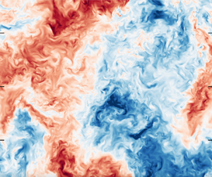
An example velocity field from the DNS of HIT is shown in figure 4, before and after the application of a spatial filter. The spatial filter may be interpreted as a form of local averaging, weighted by the filter kernel $G_\ell (\boldsymbol {r})$. Following Germano (Reference Germano1992), the generalized second moment is the difference of the filtered product and the product of two filtered fields,

(2.17)\begin{equation} \tau_\ell(a,b) = \overline{a b}^\ell - \bar{a}^\ell \bar{b}^\ell. \end{equation}

It is a generalized covariance of small-scale activity (smaller than $\ell$).

Figure 4.

The fluid velocity in the $z$ direction on an $xy$ plane in the HIT simulation: (a) unfiltered, (b) filtered at $\ell = 25\eta$ using a Gaussian filter, (3.1a,b).

The kinetic energy can be thus defined as the sum of large-scale and small-scale energies,

(2.18)\begin{equation} \tfrac{1}{2}\overline{u_i u_i}^\ell = \tfrac{1}{2}\bar{u}_i^\ell \bar{u}_i^\ell + \tfrac{1}{2}\tau_\ell(u_i, u_i). \end{equation}

If the filter kernel is positive semi-definite, i.e. $G_\ell (\boldsymbol {r}) \geq 0$ for all $\boldsymbol {r}$, then the subfilter-scale energy is positive everywhere, $\tau (u_i, u_i)(\boldsymbol {x}) \geq 0$ for all $\boldsymbol {x}$ (Vreman, Geurts & Kuerten Reference Vreman, Geurts and Kuerten1994).

Applying a low-pass filter to the incompressible Navier–Stokes equations, (2.1a,b), results in an evolution equation for the filtered velocity field,

(2.19)\begin{equation} \frac{\partial \bar{u}_i^\ell}{\partial t} + \bar{u}_j ^\ell\frac{\partial \bar{u}_i^\ell}{\partial x_j} ={-} \frac{\partial \bar{p}^\ell}{\partial x_i} + \nu \nabla^2 \bar{u}_i^\ell - \frac{\partial \tau_\ell(u_i, u_j)}{\partial x_j} + \bar{f}_i^\ell. \end{equation}

The main difference with the unfiltered Navier–Stokes equation (2.1a,b), is the introduction of the subfilter stress tensor's divergence on the right side. The dynamical equation for the large-scale kinetic energy directly follows from multiplication of (2.19) by $\bar {u}_i^\ell$,

(2.20a)\begin{equation} \frac{\partial (\tfrac{1}{2}\bar{u}_i^\ell \bar{u}_i^\ell)}{\partial t} + \frac{\partial \varPhi_j^\ell}{\partial x_j} = \bar{u}_i^\ell \bar{f}_i^\ell + \tau_\ell(u_i,u_j) \bar{S}_{ij}^\ell - 2 \nu \bar{S}_{ij}^\ell \bar{S}_{ij}^\ell, \end{equation}

where

(2.20b)\begin{equation} \varPhi_{j}^\ell = \tfrac{1}{2}\bar{u}_i^\ell \bar{u}_i^\ell \bar{u}_j^\ell + \bar{p}^\ell \bar{u}_j^\ell - 2 \nu \bar{u}_i^\ell \bar{S}_{ij}^\ell + \bar{u}_i^\ell \tau_\ell(u_i,u_j). \end{equation}

There are three source/sink terms. First, large-scale kinetic energy is produced though work done by the applied forcing function, $\bar {u}_i^\ell \bar {f}_i^\ell$. Second, the subfilter stress may add or remove energy depending on its alignment with the filtered strain-rate tensor, $\tau _\ell (u_i,u_j) \bar {S}_{ij}^\ell$. Finally, the direct dissipation of large-scale kinetic energy by viscosity, $-2\nu \bar {S}_{ij}^\ell \bar {S}_{ij}^\ell$, is typically negligible if $\ell \gg \eta$.

An equation for total kinetic energy, $\tfrac {1}{2} \overline {u_i u_i}^\ell$, is constructed by multiplying (2.1a,b) by $u_i$ and then filtering. Equation (2.20a) is subtracted from the resulting equation to form the transport equation for the small-scale energy,

(2.21a)\begin{equation} \frac{\partial ( \tfrac{1}{2}\tau_\ell(u_i,u_j) )}{\partial t} + \frac{\partial \phi_j^\ell}{\partial x_j} = \tau_\ell(u_i, f_i) - \tau_\ell(u_i, u_j) \bar{S}_{ij}^\ell - 2 \nu \tau_\ell(S_{ij}, S_{ij}), \end{equation}

where

(2.21b)\begin{equation} \phi_j^\ell = \tfrac{1}{2} \tau_\ell(u_i, u_i) \bar{u}_j^\ell + \tfrac{1}{2}\tau_\ell(u_i, u_i, u_j) + \tau_\ell(p, u_j) - 2 \nu \tau_\ell(u_i, S_{ij}), \end{equation}

where the second transport term is a generalized third moment (Germano Reference Germano1992),

(2.22)\begin{equation} \tau_\ell(a, b, c) = \overline{a b c}^\ell - \bar{a}^\ell \tau_\ell(b,c) - \bar{b}^\ell \tau_\ell(a,c) - \bar{c}^\ell \tau_\ell(a,b) - \bar{a}^\ell \bar{b}^\ell \bar{c}^\ell. \end{equation}

There are three sources/sinks in (2.21a), which have the following significance. The first source is direct forcing of the small scales, $\tau _\ell (u_i, f_i)$, which is typically negligible for $\ell \ll L$. The second is the same term, $- \tau _\ell (u_i, u_j) \bar {S}_{ij}^\ell$, as appears with opposite sign in the large-scale energy equation (2.20a). This term represents the rate at which energy is transferred from motions of size larger than $\ell$ to motions of size smaller than $\ell$. Thus, the energy cascade rate is defined as (Leonard Reference Leonard1975; Germano Reference Germano1992; Meneveau & Katz Reference Meneveau and Katz2000),

(2.23)\begin{equation} \varPi^\ell ={-} \mathring{\tau}_\ell(u_i, u_j) \bar{S}_{ij}^\ell, \end{equation}

where the overset circle indicates the deviatoric component of the tensor,

(2.24)\begin{equation} \mathring{\tau}_\ell(u_i, u_j) = \tau_\ell(u_i, u_j) - \tfrac{1}{3} \tau_\ell(u_k, u_k) \delta_{ij}. \end{equation}

The isotropic part of the subfilter stress tensor does not contribute to the energy cascade rate, $\varPi ^\ell$, because the trace of $\bar {\boldsymbol {S}}^\ell$ is zero due to incompressibility. Positive cascade rate indicates energy transfer from large to small scales and negative rate indicates backscatter or inverse cascade. It may be interpreted as the rate at which large-scale motions do work on small-scale motions (Ballouz & Ouellette Reference Ballouz and Ouellette2018).

Averaging (2.20a) and (2.21a) for a stationary, homogeneous flow yields, respectively,

(2.25)$$\begin{gather} 0 = \langle \bar{u}_i^\ell \bar{f}_i^\ell \rangle + \langle \tau_\ell(u_i,u_j) \bar{S}_{ij}^\ell \rangle - 2 \nu \langle \bar{S}_{ij}^\ell \bar{S}_{ij}^\ell \rangle, \end{gather}$$

(2.26)$$\begin{gather}0 = \langle \tau_\ell(u_i, f_i) \rangle - \langle \tau_\ell(u_i, u_j) \bar{S}_{ij}^\ell \rangle - 2 \nu \langle \tau_\ell(S_{ij}, S_{ij})\rangle. \end{gather}$$

In the inertial range of turbulence, $\eta \ll \ell \ll L$, the viscous dissipation of the large scales and forcing of the small scales may be neglected,

(2.27)\begin{equation} \langle u_i f_i \rangle \approx \langle \bar{u}_i^\ell \bar{f}_i^\ell \rangle \approx{-} \langle \tau_\ell(u_i,u_j) \bar{S}_{ij}^\ell \rangle \approx 2 \nu \langle \tau_\ell(S_{ij}, S_{ij})\rangle \approx 2 \nu \langle S_{ij} S_{ij} \rangle. \end{equation}

More simply, the inertial range is the range length scales, $\ell$, for which $\langle \varPi \rangle \approx \langle \epsilon \rangle$. Figure 5(a) tests for scales where this relation approximately holds.

Figure 5.

(a) The pre-multiplied third-order longitudinal structure function alongside the mean interscale energy transfer. (b) The average norm of the filtered strain-rate tensor as function of filter width, $\ell$. A $-2/3$ power law is consistent with inertial range behaviour. The inset is premultiplied by $\ell ^{2/3}$. In both panels, the two vertical grey lines are at $2\ell /\eta = 50$ and 150, indicating the approximate inertial range of scales. The integral length scale is $2 L / \eta = 920$.

2.5. Filtered velocity gradients

Velocity increments,

(2.28)\begin{equation} \delta u_i(\boldsymbol{r}; \boldsymbol{x}) = u_i(\boldsymbol{x}+\boldsymbol{r}) - u_i(\boldsymbol{x}) \end{equation}

and structure functions are prominent tools of classical turbulence theory. Filtered velocity gradients are intimately related to velocity increments (Eyink Reference Eyink1995),

(2.29)

where the filter kernel is assumed to be spherically symmetric. That is, the filtered velocity gradient is an averaging of velocity increments weighted by the gradient of the filter kernel. Thus, filtered velocity gradients contain information about velocity increments in the flow, arranged so as to illuminate the local topology of the flow at scale $\ell$. Filtered velocity gradients can be decomposed into rotation and deformation at scale $\ell$,

(2.30a–c)$$\begin{gather} \bar{A}_{ij}^\ell = \bar{S}_{ij}^\ell + \bar{\varOmega}_{ij}^\ell, \quad \bar{S}_{ij}^\ell = \tfrac{1}{2} ( \bar{A}_{ij}^\ell + \bar{A}_{ji}^\ell), \quad \bar{\varOmega}_{ij}^\ell = \tfrac{1}{2} ( \bar{A}_{ij}^\ell - \bar{A}_{ji}^\ell), \end{gather}$$

(2.31a,b)$$\begin{gather}\bar{\varOmega}_{ij}^\ell ={-} \tfrac{1}{2} \epsilon_{ijk} \bar{\omega}_k^\ell, \quad \bar{\omega}_i^\ell ={-} \epsilon_{ijk} \bar{\varOmega}_{jk}^\ell, \end{gather}$$

(2.32a,b)$$\begin{gather}\tfrac{1}{2} \| \bar{\boldsymbol{A}}^\ell \|^2 = \tfrac{1}{4} | \bar{\boldsymbol{\omega}}^\ell |^2 + \tfrac{1}{2}\| \bar{\boldsymbol{S}}^\ell \|^2, \quad \langle \| \bar{\boldsymbol{S}}^\ell \|^2 \rangle = \tfrac{1}{2} \langle |\bar{\boldsymbol{\omega}}^\ell|^2 \rangle. \end{gather}$$

The K41 scaling of the filtered strain-rate norm, $\|\bar {\boldsymbol {S}}^{\ell }\| \sim \ell ^{-2/3}$, is shown in figure 5(b) as another indication of what filter widths may be considered to be in the inertial range.

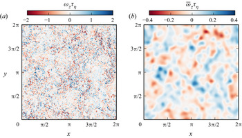
Figure 6 shows vorticity and filtered vorticity fields from the same snapshot used for figure 4. It is evident that the vorticity is predominantly organized at the smallest scales of motion, near $\eta$. This is true of the velocity gradient tensor in general. However, the filtered velocity gradient, as demonstrated for the filtered vorticity, is primarily organized at a scale near the filter width. Thus, the filtered velocity gradient provides a good definition of fluid motions at scale $\ell$. Comparing figures 4 and 6, note the striking visual difference in how filtering effects the velocity field and the velocity gradient field.

Figure 6.

The $z$ component of vorticity along the same $xy$ plane from figure 4: (a) unfiltered, (b) filtered at $\ell = 25 \eta$ using a Gaussian filter, (3.1a,b).

Like the filtered velocity gradient, the subfilter stress tensor may also be written as a local averaging of velocity increments (Constantin, E & Titi Reference Constantin, E and Titi1994; Eyink Reference Eyink1995),

(2.33)\begin{align} \tau_\ell(u_i, u_j) &= \left[ \iiint \textrm{d}\boldsymbol{r} G_\ell(\boldsymbol{r}) \delta u_i(\boldsymbol{r}; \boldsymbol{x}) \delta u_j(\boldsymbol{r}; \boldsymbol{x}) \right]\nonumber\\ &\quad - \left[ \iiint \textrm{d}\boldsymbol{r} G_\ell(\boldsymbol{r}) \delta u_i(\boldsymbol{r}; \boldsymbol{x})\right] \left[ \iiint \textrm{d}\boldsymbol{r} G_\ell(\boldsymbol{r}) \delta u_j(\boldsymbol{r}; \boldsymbol{x})\right]. \end{align}

In this way, it can be directly shown that

(2.34a,b)\begin{equation} \tau_\ell(u_i, u_j) \sim \delta u^2 \quad \text{and} \quad \bar{S}_{ij}^\ell \sim \delta u / \ell, \quad \text{therefore} \ \varPi^\ell \sim \delta u^3 / \ell, \end{equation}

so that the inertial range equation, from (2.27), in the form $\langle \varPi ^\ell \rangle = \langle \epsilon \rangle$ is in some ways analogous to the celebrated four-fifths law of Kolmogorov (Reference Kolmogorov1941a), i.e. $\langle \delta u_L^3(r) \rangle = - \tfrac {4}{5} \langle \epsilon \rangle r$. The similarity between these two is highlighted in figure 5(a), which includes the pre-multiplied third-order longitudinal structure function alongside $\langle \varPi \rangle / \langle \epsilon \rangle$. These two are similar diagnostics of inertial range scales.

2.6. Filtered velocity gradient dynamics

Definitively linking the energy cascade rate with vorticity stretching and strain self-amplification is naturally done by considering the dynamics of filtered velocity gradients. Viewing the filtered flow as the collection of fluid particles of size $\sim \ell$ following trajectories set by $\bar {\boldsymbol {u}}^\ell$, each particle's rotation and deformation dynamics may be described by the gradient of filtered Navier–Stokes, (2.19), which reads

(2.35)\begin{equation} \frac{\bar{\textrm{D}}\bar{A}_{ij}^\ell}{\overline{\textrm{D}t}} ={-} \underbrace{ \left( \bar{A}_{ik}^\ell \bar{A}_{kj}^\ell - \frac{1}{3} \bar{A}_{mn}^\ell \bar{A}_{nm}^\ell \delta_{ij} \right) }_{\mathit{autonomous\ dynamics}} - \left( \frac{\partial^2 \bar{p}^\ell}{\partial x_i x_j} - \frac{1}{3} \nabla^2 \bar{p}^\ell \delta_{ij} \right) + \nu \nabla^2 \bar{A}_{ij}^\ell - \frac{\partial \tau_\ell(u_i, u_k)}{\partial x_j \partial x_k}. \end{equation}

This equation gives the dynamical evolution of filtered velocity gradients along filtered Lagrangian trajectories, $\bar {\textrm {D}}/\overline {\textrm {D}t} = \partial /\partial t + \bar {\boldsymbol {u}}^\ell \boldsymbol {\cdot }\boldsymbol {\nabla }$. The difference from unfiltered velocity gradients, (2.8), is the gradient of the subfilter scale force. The dynamical consequence of the subfilter-scale force is subtle, and the restricted Euler-like features observed for unfiltered velocity gradients are also seen for filtered ones (Danish & Meneveau Reference Danish and Meneveau2018). In other words, the autonomous dynamics of filtered velocity gradients is very influential in setting statistical trends in turbulent flows, as previously seen for unfiltered gradients.

The restricted Euler equation for filtered velocity gradient dynamics again results by neglecting all except the autonomous terms in (2.35),

(2.36)\begin{equation} \frac{\textrm{D}}{\textrm{D}t}\left( \frac{1}{2} \| \bar{\boldsymbol{A}}^\ell \|^2 \right) = P_{\bar{\omega}} + P_{\bar{s}} = \frac{1}{4} \bar{\omega}_i^\ell \bar{S}_{ij}^\ell \bar{\omega}_j^\ell - \bar{S}_{ij}^\ell \bar{S}_{jk}^\ell \bar{S}_{ki}^\ell. \end{equation}

This, which now neglects interactions with both nearby particles and subfilter scales, highlights the role of vorticity stretching and strain self-amplification in increasing the magnitude of filtered velocity gradients. Recall from (2.32a,b) that the filtered vorticity and strain-rate are also held in statistical equi-partition by the zero divergence condition, $\boldsymbol {\nabla }\boldsymbol {\cdot }\bar {\boldsymbol {u}}^\ell = 0$, owing to the filtered pressure. In addition, the average amount of strain self-amplification is also held at three times the vorticity stretching for filtered fields,

(2.37a,b)\begin{equation} -\langle \bar{S}_{ij}^\ell \bar{S}_{jk}^\ell \bar{S}_{ki}^\ell \rangle = \tfrac{3}{4}\langle \bar{\omega}_i^\ell \bar{S}_{ij}^\ell \bar{\omega}_j^\ell \rangle \quad \text{or} \quad \langle P_{\bar{s}} \rangle = 3 \langle P_{\bar{\omega}} \rangle. \end{equation}

Equation (2.36) is only meant to demonstrate the relationship of $P_{\bar {s}}$ and $P_{\bar {\omega }}$ with the growth of filtered velocity gradients. For a full description of real turbulent flows, the pressure, viscous, and subfilter terms must be retained.

3.1. Theory

The local energy cascade rate, $\varPi (\boldsymbol {x}, t)$, is determined by the filtered strain-rate tensor, the subfilter stress tensor and how those two align. Johnson (Reference Johnson2020a) demonstrated how the subfilter stress tensor may be phrased in terms of filtered velocity gradients across all scales $\leq \ell$, so that the energy cascade rate may be written solely in terms of filtered velocity gradients. This result directly connects the restricted Euler singularity with the fact that turbulence generates a net cascade from large to small scales. A summary of the derivation is presented below, with more details provided in Appendix C.

A Gaussian filter kernel

(3.1a,b)\begin{equation} G_\ell(\boldsymbol{r}) = \mathcal{N} \exp\left( - \frac{|\boldsymbol{r}|^2}{2\ell^2}\right), \quad (2{\rm \pi})^3\mathcal{F}\{G_\ell\}(\boldsymbol{k}) = \exp\left( -\frac{1}{2} |\boldsymbol{k}|^2 \ell^2 \right), \end{equation}

decays rapidly in both physical space and wavenumber space, and is thus a popular choice for studies involving explicit filters (Borue & Orszag Reference Borue and Orszag1998; Domaradzki & Carati Reference Domaradzki and Carati2007b; Eyink & Aluie Reference Eyink and Aluie2009; Leung, Swaminathan & Davidson Reference Leung, Swaminathan and Davidson2012; Cardesa et al. Reference Cardesa, Vela-Martín, Dong and Jiménez2015; Lozano-Durán et al. Reference Lozano-Durán, Holzner and Jiménez2016; Buzzicotti et al. Reference Buzzicotti, Linkmann, Aluie, Biferale, Brasseur and Meneveau2018; Alexakis & Chibbaro Reference Alexakis and Chibbaro2020; Dong et al. Reference Dong, Huang, Yuan and Lozano-Durán2020; Portwood et al. Reference Portwood, Nadiga, Saenz and Livescu2020; Vela-Martín & Jiménez Reference Vela-Martín and Jiménez2021). Here, the definition of the filter width, $\ell$, is chosen such that its gradient, $\textrm {d}G/\textrm {d}r$, is maximum at $r=\ell$. That is, velocity increments at separation $r = \ell$ have are the most heavily weighted when constructing the filtered velocity gradient according to (2.29). Note that in figure 5(a), $2\ell$ appears to correspond to the structure function separation $r$. This happens because, in (2.29), the velocity increments with equal and opposite separation vectors of length $\ell$ are essentially combined to form velocity increments at $2\ell$, which are integrated on a half-sphere to form the filtered velocity gradient.

The Gaussian filter has already been demonstrated in physical space in figures 4 and 6. Figure 7 shows average energy spectra with and without a Gaussian filter. Note that the unfiltered spectrum decays as a (stretched) exponential in the dissipation range (Townsend Reference Townsend1951; Kraichnan Reference Kraichnan1959; Novikov Reference Novikov1961; Qian Reference Qian1984; Sreenivasan Reference Sreenivasan1985; Foias, Manley & Sirovich Reference Foias, Manley and Sirovich1990; Smith & Reynolds Reference Smith and Reynolds1991; Manley Reference Manley1992; Sanada Reference Sanada1992; Chen et al. Reference Chen, Doolen, Herring, Kraichnan, Orszag and She1993; Saddoughi & Veeravalli Reference Saddoughi and Veeravalli1994; Sirovich, Smith & Yakhot Reference Sirovich, Smith and Yakhot1994; Ishihara et al. Reference Ishihara, Kaneda, Yokokawa, Itakura and Uno2005; Khurshid, Donzis & Sreenivasan Reference Khurshid, Donzis and Sreenivasan2018; Buaria & Sreenivasan Reference Buaria and Sreenivasan2020), and the effect of the Gaussian filter moves this exponential-like decay to lower wavenumbers. The unfiltered spectrum shows agreement with the standard Kolmogorov spectrum, $E(k) = 1.6 \epsilon ^{2/3} k^{-5/3}$ over a limited range of wavenumbers $k \eta \ll 1$. A ‘spectral bump’, as typically observed, is evident near $0.1 < k\eta < 0.2$ (Qian Reference Qian1984; Falkovich Reference Falkovich1994; Lohse & Müller-Groeling Reference Lohse and Müller-Groeling1995; Kurien, Taylor & Matsumoto Reference Kurien, Taylor and Matsumoto2004; Bershadskii Reference Bershadskii2008; Frisch et al. Reference Frisch, Kurien, Pandit, Pauls, Ray, Wirth and Zhu2008; Meyers & Meneveau Reference Meyers and Meneveau2008; Mininni et al. Reference Mininni, Alexakis and Pouquet2008; Donzis & Sreenivasan Reference Donzis and Sreenivasan2010). This is usually associated with a ‘bottleneck effect’ at the end of the cascade in which viscosity is slightly too slow in dissipating energy as it arrives from larger scales, resulting in a slight pile-up of energy. While the filtering approach does smooth out this effect to some degree, it is visible for the filtered strain-rate norm in the inset of figure 5(b) in the range $5 < \ell /\eta < 10$.

Figure 7.

(a) Average energy spectrum from the HIT simulation, and (b) filtered spectra using a Gaussian filter with various values of $0.9 \eta \leq \ell \leq 170 \eta$ spaced evenly in logarithmic space. The black dashed line indicates the inertial range spectrum, $E(k) = 1.6 \epsilon ^{2/3} k^{-5/3}$. The inset in panel (a) shows the premultiplied spectrum on a log–linear plot.

Because the Gaussian kernel serves as the Green's function for the diffusion equation, a filtered quantity is the solution to

(3.2)\begin{equation} \frac{\partial \bar{a}^\ell}{\partial (\ell^2)} = \frac{1}{2} \nabla^2 \bar{a}^\ell, \quad \text{with initial condition} \ \bar{a}^{\ell=0}(\boldsymbol{x}) = a(\boldsymbol{x}), \end{equation}

where the square of the filter width, $\ell ^2$, serves as a time-like variable. The initial condition at $\ell = 0$ is the unfiltered field. From this observation, it is straightforward to show that any generalized second moment may be written as

(3.3)\begin{equation} \frac{\partial \tau_\ell(a, b)}{\partial (\ell^2)} = \frac{1}{2} \nabla^2 \tau_{\ell}(a, b) + \frac{\partial \bar{a}^\ell}{\partial x_k} \frac{\partial \bar{b}^\ell}{\partial x_k}, \quad \text{with initial condition} \ \tau_{\ell=0}(a, b) = 0. \end{equation}

Thus, the generalized second moment is the solution to a forced diffusion equation with zero initial condition. The forcing is the product of filtered gradients as a function of scale (the time-like variable). The formal solution for this forced diffusion equation is

(3.4)\begin{equation} \tau_\ell(a,b) = \int_{0}^{\ell^2} \textrm{d}\alpha \overline{\overline{\frac{\partial a}{\partial x_k}}^{\sqrt{\alpha}} \overline{\frac{\partial b}{\partial x_k}}^{\sqrt{\alpha}} }^{\beta}, \end{equation}

where $\beta \equiv \sqrt {\ell ^2 - \alpha }$ is the conjugate filter such that successively filtering at $\sqrt {\alpha }$ and $\beta$ is equivalent to applying a single filter at scale $\ell$,

(3.5)\begin{equation} \overline{\bar{a}^{\sqrt{\alpha}}}^{\beta} = \bar{a}^{\ell}. \end{equation}

The formal solution in (3.3) contains two components,

(3.6)\begin{equation} \tau_\ell(a,b) = \ell^2 \overline{\frac{\partial a}{\partial x_i}}^{\ell} \overline{\frac{\partial b}{\partial x_i}}^{\ell} + \int_{0}^{\ell^2} \textrm{d}\alpha \tau_\beta\left( \overline{\frac{\partial a}{\partial x_k}}^{\sqrt{\alpha}}, \overline{\frac{\partial b}{\partial x_k}}^{\sqrt{\alpha}} \right). \end{equation}

The first component is the product of gradients at the filter scale $\ell$ and the second component involves subfilter-scale generalized second moments of gradients filtered at scales smaller than $\ell$. Equation (3.6) is applied to the subfilter stress, $\tau _\ell (u_i, u_j)$, by setting $a = u_i$ and $b = u_j$. Contracting with $\bar {S}_{ij}^\ell$ to compute the energy cascade rate, $\varPi ^\ell$, results in

(3.7)\begin{equation} \varPi^\ell = \varPi_{s1}^\ell + \varPi_{\omega 1}^\ell + \varPi_{s2}^\ell + \varPi_{\omega 2}^\ell + \varPi_{c}^\ell. \end{equation}

The five components of (3.7) are defined and interpreted as follows.

The first two terms involve velocity gradients filtered at scale $\ell$ only. First, the self-amplification of the strain rate at scale $\ell$ transfers energy across scale $\ell$ at a rate,

(3.8)\begin{equation} \varPi_{s1}^\ell = \ell^2 P_{\bar{s}} ={-}\ell^2 \bar{S}_{ij}^\ell \bar{S}_{jk}^\ell \bar{S}_{ki}^\ell ={-}3 \ell^2 \lambda_1^\ell \lambda_2^\ell \lambda_3^\ell, \end{equation}

where $\lambda _i^\ell$ are the $3$ eigenvalues of the strain-rate tensor filtered at scale $\ell$. This term gives mathematical definition to the simplified process sketched in figure 2. The strain-rate triple product represents the production of larger strain rates with smaller spatial extent which may be thought of as similar to the dynamics of the Burgers equation. The drawing in figure 2 is meant only to provide a useful intuitive feel for how $\varPi _{s1}^\ell$ transfers energy to smaller scales, not a sweeping claim that all regions with high $\varPi _{s1}$ resemble the simplified sketch.

Similarly, the vorticity at scale $\ell$ is stretched by the strain rate at the same scale, which transfers energy

(3.9)\begin{equation} \varPi_{\omega 1}^\ell = \ell^2 P_{\bar{\omega}} = \frac{1}{4} \ell^2 \bar{S}_{ij}^\ell \bar{\omega}_{i}^\ell \bar{\omega}_j^\ell = \frac{1}{4} \ell^2 \left|\bar{\boldsymbol{\omega}}^\ell\right|^2 \sum_{i=1}^{3} \lambda_i^\ell \cos^2(\theta_{\omega,i}^\ell), \end{equation}

where $\theta _{\omega ,i}^\ell$ are the angles between each corresponding eigenvector and the vorticity vector filtered at scale $\ell$. As such, this term quantifies the local rate at which vortex stretching, as sketched in a simplified manner in figure 1, passes energy across scale $\ell$.

For these first two terms, a subscript ‘1’ is used to denote that these rates involve quantities at a single filter scale. In fact, these two terms appear both in (3.7) and in the velocity gradient evolution, (2.36). The same processes responsible for increasing the filtered velocity gradient magnitude also redistribute energy to sub-filter scales, thus connecting the restricted Euler singularity with the energy cascade. It is also possible to obtain these two as leading-order terms in an infinite expansion in at least two ways.

First, using spatial filtering with a more general filter shape, the Taylor expansion of the Leonard stress is led by these two terms (Pope Reference Pope2000). Truncation of this expansion is sometimes called the Clark model, or tensor diffusivity model (Clark, Ferziger & Reynolds Reference Clark, Ferziger and Reynolds1979; Borue & Orszag Reference Borue and Orszag1998). This model performs well in a priori tests, but does not remove large-scale energy at a sufficient rate when used with LES (Vreman, Geurts & Kuerten Reference Vreman, Geurts and Kuerten1996, Reference Vreman, Geurts and Kuerten1997). Intriguingly, it may be shown that the Lagrangian memory effects in the evolution of the subfilter stress tensor are correctly mimicked by the tensor diffusivity model (Johnson Reference Johnson2020b). In practice, the tensor diffusivity model is often supplemented with an eddy viscosity model (Clark et al. Reference Clark, Ferziger and Reynolds1979; Vreman et al. Reference Vreman, Geurts and Kuerten1996, Reference Vreman, Geurts and Kuerten1997). Eyink (Reference Eyink2006) extended this result to a multiscale gradient expansion for the full subfilter stress tensor, but still relied on truncating infinite series. Carbone & Bragg (Reference Carbone and Bragg2020) provided an alternative derivation of single-scale vorticity stretching and strain self-amplification as leading-order terms in an infinite series. In that case, the Kármán–Howarth–Monin equation (de Kármán & Howarth Reference de Kármán and Howarth1938; Monin & Yaglom Reference Monin and Yaglom1975; Hill Reference Hill2001) is used with filtered velocity gradients substituted as the leading-order term in the evaluation of velocity increments. Importantly, the result highlights agreement between velocity increment and filtering approaches to the energy cascade, indicating a degree of objectivity to this result (see, e.g. objections in Tsinober Reference Tsinober2009).

The true advantage of the result from Johnson (Reference Johnson2020a), (3.7), lies in the remaining three terms. These cascade rates involve interactions between the strain rate filtered at scale $\ell$ and velocity gradients at scales smaller than $\ell$. They are given a subscript ‘2’ to denote their multiscale nature (specifically, the sum of interactions involving two different scales). First, the cascade rate due to the amplification of small-scale strain by larger-scale strain is

(3.10)\begin{equation} \varPi_{s2}^\ell ={-} \bar{S}_{ij}^\ell \int_{0}^{\ell^2} \textrm{d}\alpha \tau_{\beta}( \bar{S}_{jk}^{\sqrt{\alpha}}, \bar{S}_{ki}^{\sqrt{\alpha}} ) ={-} \int_{0}^{\ell^2} \textrm{d}\alpha \bar{S}_{ij}^\ell \tau_{\beta}( \bar{S}_{jk}^{\sqrt{\alpha}}, \bar{S}_{ki}^{\sqrt{\alpha}} ). \end{equation}

For this term, $\bar {\boldsymbol {S}^\ell }$ represents the strain rate at the filter scale where the cascade rate is evaluated and the generalized second moment of $\bar {\boldsymbol {S}}^{\sqrt {\alpha }}$ in the integral represents smaller-scale strain rates being amplified as energy is passed down the cascade. This process may be thought of as a multiscale generalization of figure 2. Thus, $\bar{\boldsymbol {S}}^\ell$ amplifies strain rates at all scales $\sqrt {\alpha } < \ell$ and the resulting energy cascade rate is constructed by integrating over all smaller scales.

Similarly, the stretching of small-scale vorticity by larger-scale strain is

(3.11)\begin{equation} \varPi_{\omega 2}^\ell = \bar{S}_{ij}^\ell \int_{0}^{\ell^2} \textrm{d}\alpha \tau_\beta(\bar{\omega}_i^{\sqrt{\alpha}}, \bar{\omega}_j^{\sqrt{\alpha}}) = \int_{0}^{\ell^2} \textrm{d}\alpha \bar{S}_{ij}^\ell \tau_\beta(\bar{\omega}_i^{\sqrt{\alpha}}, \bar{\omega}_j^{\sqrt{\alpha}}). \end{equation}

In this mechanism, the enstrophy at scales $\sqrt {\alpha } < \ell$ is amplified as it aligns with extensional strain rates, $\boldsymbol {S}^\ell$, organized at larger scales, figure 1. This results in an energy cascade rate across scale $\ell$.

Finally, the last term in (3.7) represents the contribution to the energy cascade rate from larger-scale strain rates acting on smaller-scale strain–vorticity covariance,

(3.12)\begin{equation} \varPi_{c}^\ell = \varPi_{c2}^\ell = \bar{S}_{ij}^\ell \int_{0}^{\ell^2} \textrm{d}\alpha [ \tau_\beta( \bar{S}_{jk}^{\sqrt{\alpha}}, \bar{\varOmega}_{ki}^{\sqrt{\alpha}} ) - \tau_\beta( \bar{\varOmega}_{jk}^{\sqrt{\alpha}}, \bar{S}_{ki}^{\sqrt{\alpha}} ) ]. \end{equation}

In this final term, the strain rate at scale $\ell$ amplifies or attenuates the generalized subfilter covariance of strain rate and vorticity at all scales $\sqrt {\alpha } < \ell$. This term is given the subscript ‘$c$’, denoting it as a cross-term between both strain rate and vorticity. It is the only of the five terms not interpretable as vorticity stretching of strain self-amplification. Its meaning is less obvious, but one potential interpretation is given in § 3.3 while considering the inverse energy cascade in two dimensions.

3.3. Implications for the inverse cascade in 2-D turbulence

The main topic of this paper is the energy cascade in 3-D flows. However, it is worthwhile to comment on implications for the inverse cascade of energy in two dimensions. Of the five terms on the right side of (3.7), only the fifth term is non-zero. All vorticity stretching and strain amplification terms vanish exactly in 2-D incompressible flows. Thus

(3.13)\begin{equation} \varPi^\ell = \varPi_{c2}^\ell = \bar{S}_{ij}^\ell \int_{0}^{\ell^2} \textrm{d}\alpha [ \tau_\beta( \bar{S}_{jk}^{\sqrt{\alpha}}, \bar{\varOmega}_{ki}^{\sqrt{\alpha}} ) - \tau_\beta( \bar{\varOmega}_{jk}^{\sqrt{\alpha}}, \bar{S}_{ki}^{\sqrt{\alpha}} )]. \end{equation}

Taking the eigenframe of the strain rate at scale $\ell$,

(3.14)\begin{equation} \varPi^\ell(\boldsymbol{x}) = 2 \int_{0}^{\ell^2} \textrm{d}\alpha \iiint \textrm{d}\boldsymbol{r} G_\beta(\boldsymbol{r}) \lambda^\ell(\boldsymbol{x}) \lambda^{\sqrt{\alpha}}(\boldsymbol{x}+\boldsymbol{r}) \bar{\omega}^{\sqrt{\alpha}}(\boldsymbol{x}+\boldsymbol{r}) \sin 2 \phi(\boldsymbol{x},\boldsymbol{r}), \end{equation}

where $\phi (\boldsymbol {x},\boldsymbol {r})$ is the angle of the eigenvectors of $\bar {\boldsymbol {S}}^{\sqrt {\alpha }}(\boldsymbol {x}+\boldsymbol {r})$ with respect to the eigenvectors of $\bar {\boldsymbol {S}}^\ell (\boldsymbol {x})$. Here, the eigenvalues of the strain rate are $\lambda$ and $-\lambda$. If the strain-rate eigenvectors at $\ell$ and $\sqrt {\alpha }$ align parallel or perpendicular, then there is no transfer of energy. Maximum transfer of energy across scale $\ell$ occurs for $\pm 45^\text {o}$, with the direction of the transfer also depending on the sign of vorticity. An inverse cascade is supported when smaller-scale strain rate is misaligned with larger-scale strain rate in the opposite rotational direction as the vorticity.

One such (cartoon-ish) scenario is sketched in figure 9. As a clockwise vortex (${\omega < 0}$) is subjected to a larger-scale strain rate, it is flattened or thinned into a shear layer with strain-rate eigenvalues at $45^\circ$ from the larger-scale strain. The resulting alignment produces a maximum inverse cascade rate. This is the vortex thinning mechanism of the 2-D inverse cascade (Kraichnan Reference Kraichnan1976; Chen et al. Reference Chen, Ecke, Eyink, Rivera, Wan and Xiao2006; Xiao et al. Reference Xiao, Wan, Chen and Eyink2009).

Figure 9.

Simplified schematic of the vortex thinning mechanism driving an inverse energy cascade in 2-D turbulence.

Therefore, (3.7) represents a comprehensive view of interscale energy transfer in two- and 3-D turbulence. It is interesting to note (G.L. Eyink, private communication) that this approach may be thought of as a sort of differential renormalization group analysis (Eyink Reference Eyink2018). While vorticity stretching and (to some degree) strain self-amplification are commonly discussed as cascade mechanisms in 3-D turbulence, it should not be a surprise that the vortex thinning mechanism posited for the 2-D inverse cascade is at least a possible mechanism for energy transfer in three dimensions as well. Thus, while (3.7) from Johnson (Reference Johnson2020a) clearly identifies the roles of vorticity stretching and strain self-amplification, it also demonstrates how vortex thinning could be active, even if that activity may be negligible outside a particular range of scales in practice.

In two dimensions $\varPi _{c2}$ represents the inverse cascade. In the inertial range for 3-D turbulence, this vortex thinning term is evidently small compared with vorticity stretching and strain self-amplification, both of which drive a forward cascade to small scales. However, figure 8(a) also reveals that the vortex thinning term does provide a backscatter contribution for scales in between the viscous and inertial ranges, suggesting that the vortex thinning mechanism is a potential dynamical cause of the bottleneck effect.