1 Introduction
1.1 The ‘vapour explosion’ phenomenon in experiments
Ghelfand, Medvedev & Frolov (Reference Ghelfand, Medvedev and Frolov1988) defined the phenomenon of a sudden boiling up in situations of a high-pressure vessel decompression or the interaction of molten metal and water (Berman Reference Berman1986) as a ‘vapour explosion’. High-pressure vessel depressurization was studied in the experiments of Edwards & O’Brien (Reference Edwards and O’Brien1970) and Lienhard, Alamgir & Trela (Reference Lienhard, Alamgir and Trela1978). The tube initially contained hot water under a pressure
 $P_{0}$
greater than the pressure of saturation, and the water did not boil. In the experiment of Edwards & O’Brien,
 $P_{0}$
was greater than the pressure of saturation and the water did not boil. In the experiment of Edwards & O’Brien (Reference Edwards and O’Brien1970), the working chamber was a 4 m length tube with 7.5 cm internal diameter. The right-hand end of the tube was closed with a glass disc. Seven pressure sensors were set in the tube. In the experiments of Lienhard et al. (Reference Lienhard, Alamgir and Trela1978), the tube was 10 m long with internal diameter of 1.27 cm, but only a 2 m length section adjacent to the exit was heated. The vessel was closed with a plug kept by a cam mechanism. The pressure in the heating section was measured with two pressure sensors.
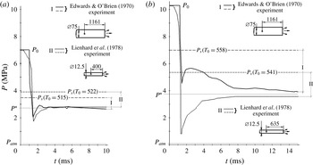
Typical pressure oscillograms from the experiments of Edwards & O’Brien (Reference Edwards and O’Brien1970) and Lienhard et al. (Reference Lienhard, Alamgir and Trela1978) are shown in figure 1. All of the oscillograms show the same wave configuration. After the vessel has been opened, the initial decompression wave goes deep into the channel with the speed of sound in a pure liquid,
 ${\sim}1000~\text{m}~\text{s}^{-1}$
. In the wave, the pressure falls below the saturation pressure but remains higher than atmospheric pressure. The wave of rarefaction is followed by a compression wave of duration 1–4 ms and 1–2 MPa amplitude. Considering that the wave configuration is moving with the sonic velocity in pure water,
 ${\sim}1000~\text{m}~\text{s}^{-1}$
, this duration of the compression wave corresponds to its 1–4 m length. Behind the wave of compression, a uniform pressure
 $P^{\ast }$
less than the pressure of saturation but greater than atmospheric pressure settles all over the vessel (
 $0.1~\text{MPa}<P^{\ast }<P_{s}(T_{0})$
). In this wave structure, the mixture converts into a state with less overheating:
 $\unicode[STIX]{x0394}T\approx T_{0}-T_{s}(P^{\ast })$
. The wave configuration as a whole has the form of a square root sign (
 $\sqrt{~}$
-type configuration).
Depressurization of tubes with different diameters
 $D$
. The experiment of Edwards & O’Brien (Reference Edwards and O’Brien1970):
 $D=7.5~\text{cm}$
, initial water parameters (a)
 $P_{0}=7~\text{MPa}$
,
 $T_{0}=515~\text{K}$
; (b)
 $P_{0}=10.3~\text{MPa}$
,
 $T_{0}=558~\text{K}$
. The experiment of Lienhard et al. (Reference Lienhard, Alamgir and Trela1978):
 $D=1.27~\text{cm}$
, initial water parameters (a)
 $P_{0}=7~\text{MPa}$
,
 $T_{0}=522~\text{K}$
; (b)
 $P_{0}=10.3~\text{MPa}$
,
 $T_{0}=541~\text{K}$
.

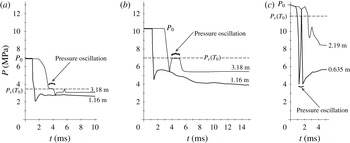
However, in the experimental material, there are oscillograms not corresponding to a general wave configuration: pressure increase up to a saturation value,
 $P_{s}(T_{0})$
, with its subsequent decrease to
 $P^{\ast }$
level. Lienhard et al. (Reference Lienhard, Alamgir and Trela1978) called this phenomenon a ‘pressure oscillation’. Such an oscillation was fixed at a cross-section of
 $x=0.914~\text{m}$
from the closed tube side (3.182 m from the opened side) in both experiments of Edwards & O’Brien (Reference Edwards and O’Brien1970) and in the third experiment of the ‘H’ series of Lienhard et al. (Reference Lienhard, Alamgir and Trela1978) at a cross-section of
 $x=0.635~\text{m}$
from the tube exit (figure 2).
Experimental pressure oscillograms from (a,b) the experiments of Edwards & O’Brien (Reference Edwards and O’Brien1970): (a)
 $P_{0}=7~\text{MPa}$
,
 $T_{0}=515~\text{K}$
; (b)
 $P_{0}=10.3~\text{MPa}$
,
 $T_{0}=558~\text{K}$
; and (c) experiment 3-H of Lienhard et al. (Reference Lienhard, Alamgir and Trela1978) with
 $P_{0}=13~\text{MPa}$
,
 $T_{0}=596~\text{K}$
. The sensor positions from the open end are shown in the figure.

Thus, the following phenomenon most apparently revealed in the second experiment of Edwards & O’Brien (Reference Edwards and O’Brien1970) can be marked. The plateau pressure level
 $P^{\ast }$
behind the compression wave is tending to a saturation one,
 $P^{\ast }\rightarrow P_{s}(T_{0})$
, as the wave propagates deep into the channel. However, the interfacial area is not sufficient to maintain the equilibrium state, as the pressure drops to a level sufficiently lower than a saturation one after the arrival of the initial rarefaction wave reflected from the closed tube end (figure 2
b).
1.2 The vapour explosion in the frame of models accounting for boiling centre origination in the flow volume
The description of flashing models, classified by the degree of detailing in simulation of the interface surface evolution, was given in our previous paper (Ivashnyov & Ivashneva Reference Ivashnyov and Ivashneva2012). There we described an equilibrium model, the SIRINGUE code model (Boivin Reference Boivin1979) and the models of Scorec & Papadimitriou (Reference Scorec, Papadimitriou, Giot, Mayinger and Celata1997) and Nigmatulin & Soplenkov (Reference Nigmatulin and Soplenkov1980). A very detailed review of flashing models is presented in the 130-page paper of Pinhasi, Ullmann & Dayan (Reference Pinhasi, Ullmann and Dayan2005). Let us describe the experiments with the model assuming boiling to start at a constant number of centres dispersed over the liquid volume (Nigmatulin & Soplenkov Reference Nigmatulin and Soplenkov1980). The number of centres per unit mixture mass
 $c$
is the only free model parameter. Among the other model assumptions are the equality of the pressures in the phases and their velocities,
 $P_{1}=P_{2}=P$
and
 $u_{1}=u_{2}=u$
, the homogeneity of the vapour parameters over a bubble volume and their equality to those on the line of saturation,
 $T_{g}=T_{s}$
,
 $\unicode[STIX]{x1D70C}_{g}=\unicode[STIX]{x1D70C}_{gs}(T_{s})$
. The subscripts ‘
 $g$
’ and ‘
 $l$
’ refer to the vapour and liquid parameters, and ‘
 $s$
’ denotes the parameters on the line of saturation.
The model consists of the continuity, momentum and energy equations for the mixture and the equation for the vapour mass balance. The interfacial area transport (IAT) equation is integrated and reduces to an algebraic equation of the constancy of the bubble number per unit mixture mass (see, for details, Ivashnyov & Ivashneva Reference Ivashnyov and Ivashneva2012):
 $$\begin{eqnarray}\frac{\unicode[STIX]{x2202}\unicode[STIX]{x1D70C}}{\unicode[STIX]{x2202}t}+\frac{\unicode[STIX]{x2202}(\unicode[STIX]{x1D70C}u)}{\unicode[STIX]{x2202}x}=0,\quad \frac{\unicode[STIX]{x2202}(\unicode[STIX]{x1D70C}u)}{\unicode[STIX]{x2202}t}+\frac{\unicode[STIX]{x2202}(\unicode[STIX]{x1D70C}u^{2}+P)}{\unicode[STIX]{x2202}x}=-\unicode[STIX]{x1D709}\frac{\unicode[STIX]{x1D70C}|u|}{2D_{ch}}u,\end{eqnarray}$$
 $$\begin{eqnarray}\frac{\unicode[STIX]{x2202}\left[\unicode[STIX]{x1D70C}\left(\text{i}-{\displaystyle \frac{P}{\unicode[STIX]{x1D70C}}}+{\displaystyle \frac{u^{2}}{2}}\right)\right]}{\unicode[STIX]{x2202}t}+\frac{\unicode[STIX]{x2202}\left[\unicode[STIX]{x1D70C}u\left(\text{i}+{\displaystyle \frac{u^{2}}{2}}\right)\right]}{\unicode[STIX]{x2202}x}=0,\quad \frac{\unicode[STIX]{x2202}(\unicode[STIX]{x1D70C}_{g}\unicode[STIX]{x1D6FD})}{\unicode[STIX]{x2202}t}+\frac{\unicode[STIX]{x2202}(\unicode[STIX]{x1D70C}_{g}\unicode[STIX]{x1D6FD}u)}{\unicode[STIX]{x2202}x}=jn,\end{eqnarray}$$
 $$\begin{eqnarray}c=n/\unicode[STIX]{x1D70C}=\text{const.},\quad \unicode[STIX]{x1D70C}=(1-\unicode[STIX]{x1D6FD})\unicode[STIX]{x1D70C}_{l}+\unicode[STIX]{x1D6FD}\unicode[STIX]{x1D70C}_{g},\quad i=(1-\unicode[STIX]{x1D712})i_{l}+\unicode[STIX]{x1D712}i_{g},\quad \unicode[STIX]{x1D712}=\frac{\unicode[STIX]{x1D70C}_{g}\unicode[STIX]{x1D6FD}}{\unicode[STIX]{x1D70C}}.\end{eqnarray}$$
Here,
 $\unicode[STIX]{x1D70C}$
,
 $\unicode[STIX]{x1D70C}_{l}$
and
 $\unicode[STIX]{x1D70C}_{g}$
are the mixture, liquid and vapour densities;
 $u$
is the flow velocity;
 $P$
is the pressure in the mixture;
 $i$
,
 $i_{l}$
and
 $i_{g}$
are the mixture, liquid and vapour enthalpies;
 $\unicode[STIX]{x1D6FD}$
and
 $\unicode[STIX]{x1D712}$
are the volumetric and mass vapour contents;
 $n$
and
 $c$
are the bubble numbers per unit mixture volume and mass;
 $D_{ch}$
is the channel diameter;
 $\unicode[STIX]{x1D709}$
is the coefficient of wall friction; and
 $j$
is the intensity of liquid evaporation into a bubble, which is determined as
 $$\begin{eqnarray}j=2\unicode[STIX]{x03C0}D_{l}a\unicode[STIX]{x1D70C}_{l}Ja\,Nu,\quad Ja=\frac{c_{l}\unicode[STIX]{x1D70C}_{l}(T_{l}-T_{s})}{\unicode[STIX]{x1D70C}_{g}h}.\end{eqnarray}$$
Here,
 $D_{l}=\unicode[STIX]{x1D706}_{l}(\unicode[STIX]{x1D70C}_{l}c_{l})^{-1}$
is the coefficient of the liquid thermal diffusivity;
 $a$
is the bubble radius;
 $Ja$
and
 $Nu$
are the Jacob and Nusselt numbers;
 $T_{l}$
and
 $T_{s}$
are the liquid and vapour temperatures;
 $h$
is the specific heat of evaporation; and
 $c_{l}$
is the specific heat capacity of the liquid.
The expression for the Nusselt number used in the model is obtained from the self-similar solution of the problem of heat bubble growth in a superheated liquid (Scriven Reference Scriven1959):
 $$\begin{eqnarray}Nu=2+\left(\frac{6Ja}{\unicode[STIX]{x03C0}}\right)^{2/3}+\frac{12Ja}{\unicode[STIX]{x03C0}}.\end{eqnarray}$$
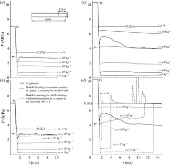
Figure 3(a,c) shows calculations of the vessel decompression under different mass concentrations of volumetrically dispersed nucleation sites,
 $c$
. Under
 $c=10^{6}~\text{kg}^{-1}$
, the predicted pressure level corresponds to the experimental one. However, the model does not simulate the 1 m length, 1 MPa amplitude compression wave following the initial decompression wave.
Experimental (Edwards & O’Brien Reference Edwards and O’Brien1970) and calculated pressure oscillograms at a cross-section of
 $x=1.116~\text{m}$
from the opened tube side under initial parameters (a,b)
 $P_{0}=7~\text{MPa}$
,
 $T_{0}=515~\text{K}$
and (c,d)
 $P_{0}=10.3~\text{MPa}$
,
 $T_{0}=558~\text{K}$
.

The fall of the pressure to significantly below the level
 $P^{\ast }$
corresponding to
 $c=10^{6}~\text{kg}^{-1}$
(figure 3
a) means that the number of bubbles which is initially much smaller than
 $10^{6}~\text{kg}^{-1}$
increases up to this value. It is reasonable to suppose this increase to be due to the bubble fragmentation. Our model accounting for bubble breakup also assumes boiling to start up at centres ‘dispersed’ in the flow volume. Its other assumptions are the same as in the model of boiling at a constant number of bubbles, except the assumption about the equality of the phase velocities, which is replaced by the assumption of smallness of the phase slip,
 $|u_{g}-u_{l}|\ll u_{l}$
. The model also includes (1.1), (1.2), but the IAT equation of (1.3a
) takes into account the bubble fragmentation. Bubble breakup is considered to be caused by Kelvin–Helmholtz instability induced by bubbles overflowing:
 $$\begin{eqnarray}\frac{\unicode[STIX]{x2202}n}{\unicode[STIX]{x2202}t}+\frac{\unicode[STIX]{x2202}(nu)}{\unicode[STIX]{x2202}x}=\unicode[STIX]{x1D70C}\unicode[STIX]{x1D713},\quad \unicode[STIX]{x1D713}=\frac{c^{\ast }-c}{\unicode[STIX]{x1D70F}^{\ast }},\end{eqnarray}$$
 $$\begin{eqnarray}\frac{c^{\ast }}{c}=\frac{We}{We^{\ast }},\quad \unicode[STIX]{x1D70F}^{\ast }=\sqrt{\frac{\unicode[STIX]{x1D70C}_{l}a^{3}}{\unicode[STIX]{x1D70E}}\left(\frac{We}{We^{\ast }}\right)^{3}},\end{eqnarray}$$
where
 $\unicode[STIX]{x1D713}$
is the intensity of bubble breakup which is defined with a relaxation ratio;
 $n^{\ast }$
is the number of bubbles that would be formed if the fragmentation were instantaneous, and
 $\unicode[STIX]{x1D70F}^{\ast }$
is the characteristic fragmentation time;
 $\unicode[STIX]{x1D70E}$
is the coefficient of the surface tension;
 $We$
and
 $We^{\ast }$
are the Weber number and its critical value.
The Weber number is defined in terms of the vapour density
 $\unicode[STIX]{x1D70C}_{g}$
as
 $$\begin{eqnarray}We=\frac{2a\unicode[STIX]{x1D70C}_{g}(u_{g}-u_{l})^{2}}{\unicode[STIX]{x1D70E}}.\end{eqnarray}$$
Its critical value chosen for calculations,
 $We^{\ast }=1$
, corresponds to
 $We^{\ast }\sim 100$
in terms of liquid density.
The difference in phase velocities in the equation for
 $We$
is determined with the equation of motion of an individual dispersed unit (Drew & Passman Reference Drew and Passman1998):
 $$\begin{eqnarray}(\unicode[STIX]{x1D70C}_{g}+C_{vm}\unicode[STIX]{x1D70C}_{l})\frac{\text{D}_{g}u_{g}}{\text{D}t}=\unicode[STIX]{x1D70C}_{l}(1+C_{vm})\frac{\text{D}u}{\text{D}t}-\frac{3}{a}C_{vm}\unicode[STIX]{x1D70C}_{l}(u_{g}-u)\frac{\text{D}_{g}a}{\text{D}t}-S(u_{g}-u),\end{eqnarray}$$
 $$\begin{eqnarray}S=\frac{3}{8a}c_{\unicode[STIX]{x1D707}}\unicode[STIX]{x1D70C}_{l}|u_{g}-u|,\quad \frac{\text{D}}{\text{D}t}=\frac{\unicode[STIX]{x2202}}{\unicode[STIX]{x2202}t}+u\frac{\unicode[STIX]{x2202}}{\unicode[STIX]{x2202}x},\quad \frac{\text{D}_{g}}{\text{D}t}=\frac{\unicode[STIX]{x2202}}{\unicode[STIX]{x2202}t}+u_{g}\frac{\unicode[STIX]{x2202}}{\unicode[STIX]{x2202}x},\end{eqnarray}$$
where
 $C_{vm}$
is the virtual mass coefficient, equal to
 $1/2$
for spherical bubbles;
 $S$
is the drag force per unit velocity;
 $c_{\unicode[STIX]{x1D707}}$
is the drag coefficient;
 $a$
is the bubble radius;
 $\text{D}/\text{D}t$
is the material derivative following the mixture (following the liquid, as
 $u\approx u_{l}$
according to the model assumption);
 $\text{D}_{g}/\text{D}t$
is the material derivative following the bubbles. (The analysis of the terms on the right-hand side of (1.9) is given in § 5.3.)
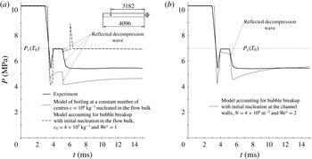
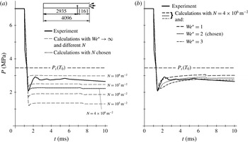
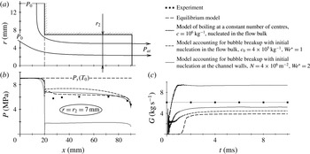
Comparison of the experimental and theoretical pressure oscillograms at a cross-section 3.182 m distant from the opened channel end for the initial conditions of the second experiment of Edwards & O’Brien (Reference Edwards and O’Brien1970) (
 $P_{0}=10.3~\text{MPa}$
,
 $T_{0}=558~\text{K}$
). (a) The models accounting for boiling nucleation in the flow bulk at a constant number of bubbles and accounting for bubble breakup. (b) The model accounting for nucleation at the channel walls and bubble breakup.

Figure 3(b,d) shows the oscillograms obtained with the model accounting for bubble breakup with different numbers of boiling centres
 $c_{0}$
and fixed
 $We^{\ast }=1$
. (The same meaning of the critical Weber number was specified for all calculations in Ivashnyov, Ivashneva & Smirnov (Reference Ivashnyov, Ivashneva and Smirnov2000) and Ivashnyov & Ivashneva (Reference Ivashnyov and Ivashneva2012).) The best correspondence with the experiment is attained under
 $c_{0}=4\times 10^{5}~\text{kg}^{-1}$
(figure 3
b).
For the conditions of the first experiment of Edwards & O’Brien (Reference Edwards and O’Brien1970), the model does not predict bubble fragmentation (figure 3 b), and the calculated curves practically coincide with the predictions of the model of boiling at a constant number of centres (figure 3 a).
Under the conditions of the second experiment, the model shows that the pressure ‘overjumping’
 $P^{\ast }$
increases up to a saturation level
 $P_{s}(T_{0})$
(figure 3
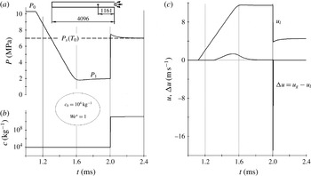
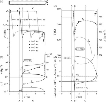
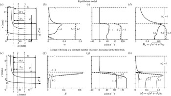
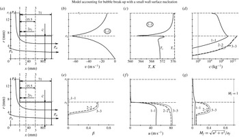
d). Figure 5 shows the structure of this compression wave. Its arrival causes the increase in the difference in the phase velocities which reaches
 $18~\text{m}~\text{s}^{-1}$
(figure 5
c). The bubbles start to fragment intensively and their number increases by orders of magnitude, up to
 $10^{11}~\text{kg}^{-1}$
(figure 5
b). Due to the interfacial surface enlargement, the boiling mixture transforms into an equilibrium state. The equilibrium boiling keeps the pressure behind the wave at a level of
 $P_{s}(T_{l})$
and ‘maintains’ the compression wave. The wave is thus a ‘self-sustaining’ one, i.e. detonation type. (The structure of the detonation wave can be investigated using a stationary version of model (1.1), (1.2), (1.6), (1.9) in the coordinate system linked with the wave, as has been done for a rarefaction wave of boiling (Ivashnyov et al.
Reference Ivashnyov, Ivashneva and Smirnov2000; Ivashnyov & Ivashneva Reference Ivashnyov and Ivashneva2012). The breakup of the bubbles located in the flow volume causes the boiling intensification and pressure increase that results in an essential increase in the phase slip. The Weber number (1.8) increases in spite of the diminution of the bubble sizes, and the breakup is repeated, i.e. it proceeds in a chain mode and only comes to an end when the mixture reaches the equilibrium, which explains the increase in the number of bubbles by eight orders of magnitude in the wave.)
Calculations using the model accounting for bubble breakup with the initial nucleation in the flow bulk (Ivashnyov et al.
Reference Ivashnyov, Ivashneva and Smirnov2000) with free model parameters of
 $c_{0}=10^{4}~\text{kg}^{-1}$
,
 $We^{\ast }=1$
. (a–c) Dependences versus time of (a) the pressure, (b) the bubble number, and (c) the flow velocity and phase slip at cross-section
 $x=1.116~\text{m}$
from the opened tube end. The initial flow parameters are
 $P_{0}=10.3~\text{MPa}$
,
 $T_{0}=558~\text{K}$
.

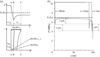
The detonation wave can be interpreted as a ‘rising’ part of the pressure oscillation fixed in the experiment (figure 2
b). However, according to calculations, the ‘decreasing’ part is not formed: the pressure continues to stay at the level of saturation. It lacks a reverse transfer into an overheated state after a reflected wave arrival (figure 4
a). The reason is that the part of the initial decompression wave
 $P_{0}$
–
 $P_{s}(T_{0})$
attenuates practically at once after reflection and does not interact with the wave propagating towards the closed side. The part of the wave configuration consisting of the pressure undershoot
 $P_{s}(T_{0})$
–
 $P_{min}$
and its subsequent increase up to
 $P_{s}(T_{0})$
transforms, after reflection, into a peak above
 $P_{s}(T_{0})$
clearly seen in figure 3(d).
Accuracy of the flashing flow simulations.

To simulate flashing, Edwards (Reference Edwards1968) proposed a model with two free parameters. Besides the number of bubbles per unit liquid mass, the time delay in bubble nucleation was specified. The parameters were adjusted to obtain the pressure plateau
 $P^{\ast }$
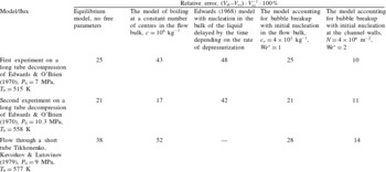
level observed at an initial stage of decompression (figure 1). (The errors of the main stage simulation are given in table 1 in § 7.3.) Introducing the time delay, Edwards & O’Brien (Reference Edwards and O’Brien1970) managed to simulate the pressure undershoot with its subsequent increase up to
 $P^{\ast }$
in the cross-section of 1.16 m for both experiments. However, the model did not describe the pressure curve in the cross-section of 3.18 m with the pressure oscillation up to a saturation level.
Developing our model (Ivashniov & Soplenkov Reference Ivashniov and Soplenkov1992) accounting for bubble breakup due to Kelvin–Helmholtz instability, Pinhasi et al. (Reference Pinhasi, Ullmann and Dayan2005) additionally considered the bubble breaking mechanism attributed to Rayleigh–Taylor instability caused by the liquid acceleration. These authors made the conclusion that these two types of instabilities give equal contributions in the bubble breakup processes at the initial stages of decompression. In Pinhasi et al. (Reference Pinhasi, Ullmann and Dayan2005), the model predictions are compared with the experimental results of Bartak (Reference Bartak1990) on the decompression of a 1.7 m tube connected with a tank, but the modelling of the Edwards & O’Brien (Reference Edwards and O’Brien1970) experiments is not presented.
The scheme of phase interface shaping.

Ivashnev & Smirnov (Reference Ivashnev and Smirnov2005) independently proposed a model accounting for bubble breakup induced by Rayleigh–Taylor instability. The model, as all of the previous ones, assumes boiling to start at the centres dispersed in the liquid bulk. The initial decompression stage simulation has shown that the model gives the same results as the model of Ivashnyov et al. (Reference Ivashnyov, Ivashneva and Smirnov2000) accounting for Kelvin–Helmholtz instability and initial nucleation in the flow bulk, which predicts either no fragmentation (figure 3 b) or too intensive chain fragmentation (figure 3 d).
2 Hypothesis on flashing inception
The idea of Edwards (Reference Edwards1968) about the time delay in bubble nucleation in the flow bulk as a key factor for simulating 1 MPa pressure increase in the compression wave up to
 $P^{\ast }$
level,
 $P^{\ast }<P_{s}(T_{0})$
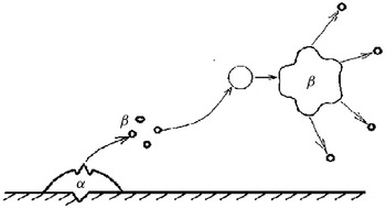
, seems to be the most constructive. A physical mechanism that could ensure the delay could be the initial formation of bubbles on the channel walls. Figure 6 shows the scheme of the phase interface evolution: a speed flow breaks wall surface bubbles, carrying their fragments into its core; after growing up, ‘in-flow’ bubbles are breaking in their turn.
Having analysed different ways of nucleation, Riznic & Ishii (Reference Riznic and Ishii1989) also came to the conclusion that, in flashing flow, initial nucleation proceeds at channel walls, and proposed a model with a bubble number transport equation analogous to (1.6), which had a source term due to bubble departures from walls. The departure frequency was determined from the dependences proposed by Kocamustafaogullari & Ishii (Reference Kocamustafaogullari and Ishii1983) for slow flows in heated channels (pool boiling). The model of Riznic & Ishii (Reference Riznic and Ishii1989) described the vapour content profiles from Reocreux’s (Reference Reocreux1978) and BNL (Wu & Abuaf Reference Wu, Abuaf and Saha1981) nozzle experiments that evidenced in favour of wall nucleation in flashing flow.
3 In-volume initial bubble origination versus wall boiling up
Attempts to answer the question of where the initial bubbles arise experimentally, at channel walls or in the flow volume, give discrepant results. Judging from the lack of a critical mass flux dependence on the tube diameter, Ogasawara (Reference Ogasawara1969) concluded that boiling nucleation occurred in the flow volume. However, experiments on long nozzles showed a dependence of the critical mass flux on the channel diameter. Boivin (Reference Boivin1979) found increase in the mass flux with increasing diameter and concluded that boiling centres are formed at the wall surface. However, Sozzi & Sutherland (Reference Sozzi and Sutherland1975) found an opposite diameter effect.
In our previous paper (Ivashnyov & Ivashneva Reference Ivashnyov and Ivashneva2012), the experiments of Boivin (Reference Boivin1979) on flows in nozzles with different diameters were reproduced with a high accuracy by a model accounting for bubble breakup, using the same free parameter, the initial number of boiling centres in the flow volume. It was shown that the mass flow rate was determined by the bubble fragmentation, causing the increase in the bubble number by orders of magnitude. Since breaking is governed by a lot of factors, the link between the initial bubble number and the boiling intensity is lost. That is, it does not seem reasonable to determine the location of the initial boiling centres from the dependence of the critical mass flow rate on the channel diameter.
The question about the bubble origination might be answered experimentally from the dependence of the pressure undershoot on the tube diameter under the tube decompression, since boiling is the only reason why the pressure does not drop to atmospheric pressure. However, we did not manage to find experiments with different tube diameters and completely identical initial water parameters, liquid purity, wall smoothness and rate of decompression.
From the pressure profiles, recorded in experiments on saturated water efflux through a short tube with a sharp right-angled entrance (appendix A), Tikhonenko et al. (Reference Tikhonenko, Kevorkov and Lutovinov1979) concluded that the stream was separated from the walls at the channel input, continued to narrow up to the cross-section 0.5 calibre distance and then expanded, filling all of the tube. At that point, the mass flow rate was close to that for an equilibrium mixture. Nigmatulin (Reference Nigmatulin1991) interpreted these results as evidence of liquid beginning to boil without contact with the walls, i.e. in the flow bulk.
However, since the water in the tank was saturated, the possibility of boiling up at the tank walls upstream of the tube entrance cannot be excluded. In appendix A, the experiments of Tikhonenko et al. (Reference Tikhonenko, Kevorkov and Lutovinov1979) are calculated with a model based on the assumption that the initial boiling centres are located at a wall surface. The calculations show that, near the tank walls, the pressure decreases due to fluid motion, the temperature of saturation also decreases, the liquid overheating increases to 15 K, and wall bubbles are formed. On growing up to critical dimensions, they break up, with the fragments released into the liquid layer flowing over the tank walls. As a result, on entering the pipe, the stream already contains a lot of nucleation centres. At that point, because of their microscopic dimensions, the volumetric vapour fraction is negligibly small,
 $4\times 10^{-3}$
, and the stream is constricted as a pure fluid is. Thus, the experimental results of Tikhonenko et al. (Reference Tikhonenko, Kevorkov and Lutovinov1979) do not prove an in-volume origination of boiling centres.
Therefore, there is no direct evidence of boiling up in the flow bulk for a high-speed flow.
Let us consider the results of the experiments on boiling up in bubble chambers with a motionless fluid separated from the walls. In the work of Scripov (Reference Scripov1972), a formula is given that generalizes experiments carried with all the liquids available at that time. It gives the probability of the formation of boiling centres due to intermolecular tier breakup in a unit of volume per unit time (the rate of a homogeneous nucleation):
 $$\begin{eqnarray}\unicode[STIX]{x1D713}=\unicode[STIX]{x1D713}_{\ast }\exp (-Gi),\quad Gi=\frac{16\unicode[STIX]{x03C0}\unicode[STIX]{x1D70E}^{3}}{3kT_{l}(P_{s}-P_{l})^{2}(1-\unicode[STIX]{x1D70C}_{g}/\unicode[STIX]{x1D70C}_{l})^{2}},\end{eqnarray}$$
where
 $\unicode[STIX]{x1D713}_{\ast }$
in the first approximation is considered to be a constant depending on the type of liquid (
 $\unicode[STIX]{x1D713}_{\ast }\sim 10^{38}~\text{m}^{-3}~\text{s}^{-1}$
for water). Here,
 $Gi$
is the Gibbs number;
 $k=1.381\times 10^{-23}~\text{J}~\text{K}^{-1}$
is the Boltzmann constant;
 $P_{s}-P_{l}$
is the difference in the pressures in the saturated vapour and in the liquid.
The rate of nucleation evaluated for water at zero pressure (that is under the most favourable conditions for the breakup of intermolecular ties) is
 $$\begin{eqnarray}Gi\approx 10\,000,\quad \unicode[STIX]{x1D713}(T_{l}=590~\text{K},P_{l}=0)=10^{-6}~\text{m}^{-3}~\text{s}^{-1}.\end{eqnarray}$$
In the experiments of Edwards & O’Brien (Reference Edwards and O’Brien1970), the efflux process takes a time not exceeding a second. Therefore, according to (3.1), no one bubble can appear in the whole vessel during the experiment. The probability of in-volume boiling centre origination only arises near a critical point. (For water,
 $T_{cr}=647.3~\text{K}$
.)
Where do boiling sites in such a quantity as
 $10^{6}~\text{kg}^{-1}$
(figure 3) come from in a ‘demineralized water degassed under vacuum’ (Edwards & O’Brien Reference Edwards and O’Brien1970) or ‘degassed by boiling double-distilled water’ (Lienhard et al.
Reference Lienhard, Alamgir and Trela1978)? The only possibility for centres to arise is nucleation at channel walls.
4 The problem of the non-hyperbolic character of a two-phase two-velocity model and its solution
4.1 Estimation of the phase slips in the wave of compression
Let us show that, in compression waves, the phase slip can reach appreciable values. The characteristic time for a wavy processes,
 $\unicode[STIX]{x1D70F}^{\ast }$
, can be evaluated as
 $$\begin{eqnarray}\unicode[STIX]{x1D70F}^{\ast }\sim \frac{L^{\ast }}{a_{l}^{\ast }}\sim 10^{-3}~\text{s}\ll \frac{L^{\ast }}{u_{l}^{\ast }}\sim 10^{-1}~\text{s},\quad u_{l}^{\ast }=\frac{P_{0}-P^{\ast }}{\unicode[STIX]{x1D70C}_{l}^{\ast }a_{l}^{\ast }}\sim 10~\text{m}~\text{s}^{-1},\end{eqnarray}$$
where
 $L^{\ast }\sim 1~\text{m}$
is the characteristic length of the compression wave;
 $a_{l}^{\ast }\sim 1000~\text{m}~\text{s}^{-1}$
is the speed of sound in liquid;
 $u_{l}^{\ast }$
is the liquid velocity behind the wave front.
Under condition (4.1), the convective components of substantial derivatives with respect to time in the equation for single bubble motion (1.9) can be neglected. Neglecting vapour density compared with that of the liquid
 $(\unicode[STIX]{x1D70C}_{g}\ll \unicode[STIX]{x1D70C}_{l})$
, too, we obtain the equation for the phase slip,
 $\unicode[STIX]{x0394}u=u_{g}-u_{l}$
, in the form
 $$\begin{eqnarray}\frac{\unicode[STIX]{x2202}(\unicode[STIX]{x0394}u)}{\unicode[STIX]{x2202}t}=2\frac{\unicode[STIX]{x2202}u}{\unicode[STIX]{x2202}t}-\frac{3}{a}\unicode[STIX]{x0394}u\frac{\unicode[STIX]{x2202}a}{\unicode[STIX]{x2202}t}-\frac{3}{8a}C_{\unicode[STIX]{x1D707}}|\unicode[STIX]{x0394}u|\unicode[STIX]{x0394}u.\end{eqnarray}$$
In compression waves, the two first terms on the right-hand side of (4.2) lead to an increase in the absolute value of the difference in the phase velocities. The first term, which is the rate of the velocity decreasing in the compression wave, results in an increase of the absolute value of the negative phase slip. The second term represents how, in a compression wave, bubbles collapse (
 $\unicode[STIX]{x2202}a/\unicode[STIX]{x2202}t<0$
), lose their virtual mass and the absolute value of the difference in phase velocities increases. The last term, the interfacial drag force, always diminishes the phase slip. The difference in the phase velocities
 $\unicode[STIX]{x0394}u$
will stop increasing as soon as the last term reaches a value equal to the sum of absolute values of the first two terms.
When the difference in phase velocities has the same order of magnitude as the velocity,
 $$\begin{eqnarray}\unicode[STIX]{x0394}u\sim u,\end{eqnarray}$$
all three terms on the right-hand side of (4.2) are of the same order:
 $$\begin{eqnarray}\frac{\unicode[STIX]{x2202}u}{\unicode[STIX]{x2202}t}\sim \frac{u^{\ast }}{\unicode[STIX]{x1D70F}^{\ast }}\sim \frac{\unicode[STIX]{x0394}u}{a}\frac{\unicode[STIX]{x2202}a}{\unicode[STIX]{x2202}t}\sim \frac{|\unicode[STIX]{x0394}u|}{\unicode[STIX]{x1D70F}^{\ast }}\sim \frac{(\unicode[STIX]{x0394}u)^{2}}{a}C_{\unicode[STIX]{x1D707}}\sim 10^{4}~\text{m}~\text{s}^{-2}.\end{eqnarray}$$
Estimation (4.4) is obtained taking into account supposition (4.3) and evaluations (4.1) for
 $\unicode[STIX]{x1D70F}^{\ast }$
,
 $u_{l}^{\ast }\approx u^{\ast }$
. The bubble radius is estimated to be
 $a\sim 10^{-4}~\text{m}$
from experimental liquid overheats and
 $\unicode[STIX]{x1D70F}^{\ast }$
. The bubble Reynolds number is estimated as
 $Re\sim 10^{4}$
from the bubble radius and
 $\unicode[STIX]{x0394}u$
;
 $C_{\unicode[STIX]{x1D707}}(Re)\sim 4\times 10^{-2}$
is taken from Schlichting (Reference Schlichting1964).
Therefore, the interfacial drag forces are rather small, and the difference in the phase velocities in the compression wave can reach values comparable with the flow velocity. The situation
 $|\unicode[STIX]{x0394}u|\sim u$
did take place in calculations with the model of Ivashnyov et al. (Reference Ivashnyov, Ivashneva and Smirnov2000) shown in figure 5(c). Thus, as it is based on the assumption that
 $|u_{g}-u|\ll u$
, the model goes beyond its validity limits. In order to calculate compression waves in bubbly media one needs to abandon the assumption.
Unfortunately, the known models for two-velocity two-phase flow with a compressible carrying phase do not permit one to simulate correctly the flow with phase slip comparable to the flow velocity. These models are named by different authors as ‘non-hyperbolic’ (Nigmatulin Reference Nigmatulin1991), ‘non-evolutionary’ (Kulikovskii & Shikina Reference Kulikovskii and Shikina1996), ‘incorrect’ (Crayko Reference Crayko1982), ‘non-stable’ (Gear Reference Gear1971; Lahey et al. Reference Lahey, Cheng, Drew and Flaherty1980), etc.
4.2 The requirements for the model of a compressible medium in mathematical terms
For any compressible medium, the velocity of the small perturbations spreading, the sound velocity, must be finite. In mathematical terms, this finiteness means that the model is hyperbolic. A hyperbolic model is one that has only real mathematical characteristics. In essence, the characteristics are the lines in
 $(t,x)$
coordinates along which small high-frequency perturbations are spread. Any hyperbolic system can be rewritten in an equivalent characteristic form, i.e. as a system of the equations for characteristic lines and invariants preserved along them.
For the simplest model of ideal gas adiabatic flow,
 $$\begin{eqnarray}\frac{\unicode[STIX]{x2202}\unicode[STIX]{x1D70C}}{\unicode[STIX]{x2202}t}+\frac{\unicode[STIX]{x2202}(\unicode[STIX]{x1D70C}u)}{\unicode[STIX]{x2202}x}=0,\quad \frac{\unicode[STIX]{x2202}u}{\unicode[STIX]{x2202}t}+u\frac{\unicode[STIX]{x2202}u}{\unicode[STIX]{x2202}x}+\frac{1}{\unicode[STIX]{x1D70C}}\frac{\unicode[STIX]{x2202}P}{\unicode[STIX]{x2202}x}=0,\quad \frac{P}{\unicode[STIX]{x1D70C}^{\unicode[STIX]{x1D6FE}}}=\text{const.},\end{eqnarray}$$
the characteristic form is the system of Riemann invariants,
 $$\begin{eqnarray}\displaystyle & \displaystyle \frac{\unicode[STIX]{x2202}}{\unicode[STIX]{x2202}t}\left(\frac{2a_{g}}{\unicode[STIX]{x1D6FE}-1}+u\right)+(u+a_{g})\frac{\unicode[STIX]{x2202}}{\unicode[STIX]{x2202}x}\left(\frac{2a_{g}}{\unicode[STIX]{x1D6FE}-1}+u\right)=0,\quad a_{g}=\sqrt{\unicode[STIX]{x1D6FE}\frac{P}{\unicode[STIX]{x1D70C}}}, & \displaystyle\end{eqnarray}$$
 $$\begin{eqnarray}\displaystyle & \displaystyle \frac{\unicode[STIX]{x2202}}{\unicode[STIX]{x2202}t}\left(\frac{2a_{g}}{\unicode[STIX]{x1D6FE}-1}-u\right)+(u-a_{g})\frac{\unicode[STIX]{x2202}}{\unicode[STIX]{x2202}x}\left(\frac{2a_{g}}{\unicode[STIX]{x1D6FE}-1}-u\right)=0, & \displaystyle\end{eqnarray}$$
where
 $\unicode[STIX]{x1D70C}$
,
 $P$
and
 $u$
are the density, pressure and velocity of an ideal gas;
 $\unicode[STIX]{x1D6FE}$
is the adiabatic curve exponent;
 $a_{g}$
is the speed of sound in gas.
It follows from (4.6) that, along the first characteristic, the line
 $\text{d}x/\text{d}t=u+a_{g}$
, the first Riemann invariant is preserved, the complex of parameters
 $2a_{g}/(\unicode[STIX]{x1D6FE}-1)+u=\text{const.}$
Alternatively,
 $$\begin{eqnarray}\frac{\text{d}_{1}}{\text{d}t}\left(\frac{2a_{g}}{\unicode[STIX]{x1D6FE}-1}+u\right)=0,\quad \frac{\text{d}_{1}}{\text{d}t}=\frac{\unicode[STIX]{x2202}}{\unicode[STIX]{x2202}t}+(u+a_{g})\frac{\unicode[STIX]{x2202}}{\unicode[STIX]{x2202}x}.\end{eqnarray}$$
The second invariant,
 $2a_{g}/(\unicode[STIX]{x1D6FE}-1)-u=\text{const.}$
, is preserved along the second characteristic
 $\text{d}x/\text{d}t=u-a_{g}$
,
 $$\begin{eqnarray}\frac{\text{d}_{2}}{\text{d}t}\left(\frac{2a_{g}}{\unicode[STIX]{x1D6FE}-1}-u\right)=0,\quad \frac{\text{d}_{2}}{\text{d}t}=\frac{\unicode[STIX]{x2202}}{\unicode[STIX]{x2202}t}+(u-a_{g})\frac{\unicode[STIX]{x2202}}{\unicode[STIX]{x2202}x}.\end{eqnarray}$$
4.3 Characteristics of a ‘classic’ model for two-phase two-velocity flow
Following Lahey et al. (Reference Lahey, Cheng, Drew and Flaherty1980), let us consider the generally adopted ‘dirty water’ model of a fluid with incompressible particles. Let the fluid be compressible with a linear equation of state. The model consists of two equations for mass and two ‘symmetrical’ equations for momentum:
 $$\begin{eqnarray}\frac{\unicode[STIX]{x2202}[\unicode[STIX]{x1D70C}_{l}(1-\unicode[STIX]{x1D6FD})]}{\unicode[STIX]{x2202}t}+\frac{\unicode[STIX]{x2202}[\unicode[STIX]{x1D70C}_{l}(1-\unicode[STIX]{x1D6FD})u_{l}]}{\unicode[STIX]{x2202}x}=0,\quad \frac{\unicode[STIX]{x2202}[\unicode[STIX]{x1D70C}_{g}\unicode[STIX]{x1D6FD}]}{\unicode[STIX]{x2202}t}+\frac{\unicode[STIX]{x2202}[\unicode[STIX]{x1D70C}_{g}\unicode[STIX]{x1D6FD}u_{g}]}{\unicode[STIX]{x2202}x}=0,\end{eqnarray}$$
 $$\begin{eqnarray}\unicode[STIX]{x1D70C}_{l}(1-\unicode[STIX]{x1D6FD})\frac{\text{D}_{l}u_{l}}{\text{D}t}=-(1-\unicode[STIX]{x1D6FD})\frac{\unicode[STIX]{x2202}P}{\unicode[STIX]{x2202}x}+M_{l}-(1-\unicode[STIX]{x1D6FD})F_{w},\quad \unicode[STIX]{x1D70C}_{l}\unicode[STIX]{x1D6FD}\frac{\text{D}_{g}u_{g}}{\text{D}t}=-\unicode[STIX]{x1D6FD}\frac{\unicode[STIX]{x2202}P}{\unicode[STIX]{x2202}x}+M_{g}-\unicode[STIX]{x1D6FD}F_{w},\end{eqnarray}$$
 $$\begin{eqnarray}M_{l}=-M_{g}=-n(1-\unicode[STIX]{x1D6FD})f_{vm}-\unicode[STIX]{x1D6FD}(1-\unicode[STIX]{x1D6FD})S(u_{g}-u_{l}),\end{eqnarray}$$
 $$\begin{eqnarray}\unicode[STIX]{x1D6FD}=\frac{4\unicode[STIX]{x03C0}a^{3}}{3}n,\quad \frac{1}{\unicode[STIX]{x1D70C}_{l}}=k-\frac{P}{\unicode[STIX]{x1D6FD}_{l}^{2}},\quad k,\quad \unicode[STIX]{x1D6FD}_{l}=\text{const.},\quad a=\text{const.},\quad \unicode[STIX]{x1D70C}_{g}=\text{const.},\end{eqnarray}$$
 $$\begin{eqnarray}\frac{\text{D}_{l}}{\text{D}t}=\frac{\unicode[STIX]{x2202}}{\unicode[STIX]{x2202}t}+u_{l}\frac{\unicode[STIX]{x2202}}{\unicode[STIX]{x2202}x},\quad \frac{\text{D}_{g}}{\text{D}t}=\frac{\unicode[STIX]{x2202}}{\unicode[STIX]{x2202}t}+u_{g}\frac{\unicode[STIX]{x2202}}{\unicode[STIX]{x2202}x},\end{eqnarray}$$
 $$\begin{eqnarray}f_{vm}=\frac{2}{3}\unicode[STIX]{x03C0}a^{3}\unicode[STIX]{x1D70C}_{l}a_{vm},\quad a_{vm}=-\left(\frac{\text{D}_{g}u_{g}}{\text{D}t}-\frac{\text{D}_{l}u_{l}}{\text{D}t}\right),\end{eqnarray}$$
where
 $a$
is the particle radius;
 $\unicode[STIX]{x1D70C}_{l}$
and
 $\unicode[STIX]{x1D70C}_{g}$
are the densities of the fluid and particles;
 $u_{l}$
and
 $u_{g}$
are the phase velocities;
 $\unicode[STIX]{x1D6FD}$
is the volumetric vapour content;
 $P$
is the pressure in the fluid;
 $M_{l}$
and
 $M_{g}$
are the interfacial area forces for the liquid and particles;
 $F_{w}$
is the wall shear force per unit mixture volume;
 $n$
is the number of particles per unit mixture volume;
 $S$
is the drag force per unit velocity given by (1.10);
 $f_{vm}$
is the virtual mass force;
 $a_{vm}$
is the virtual mass acceleration;
 $\unicode[STIX]{x1D6FD}_{l}$
is the coefficient of the liquid compressibility;
 $\text{D}_{l}/\text{D}t$
and
 $\text{D}_{g}/\text{D}t$
are the material derivatives following the liquid and the particles.
A standard procedure of characteristic searching gives an algebraic equation of the fourth order:
 $$\begin{eqnarray}y^{4}-2\frac{\unicode[STIX]{x0394}u}{a_{l}}y^{3}+\left[\left(\frac{\unicode[STIX]{x0394}u}{a_{l}}\right)^{2}-\frac{(1+2\unicode[STIX]{x1D6FD})\unicode[STIX]{x1D70C}_{l}+2(1-\unicode[STIX]{x1D6FD})\unicode[STIX]{x1D70C}_{g}}{(1-\unicode[STIX]{x1D6FD})(\unicode[STIX]{x1D70C}_{l}+(2+\unicode[STIX]{x1D6FD})\unicode[STIX]{x1D70C}_{g})}\right]y^{2}+2\frac{\unicode[STIX]{x0394}u}{a_{l}}ky-\left(\frac{\unicode[STIX]{x0394}u}{a_{l}}\right)^{2}k=0,\end{eqnarray}$$
 $$\begin{eqnarray}y=\frac{1}{a_{l}}\left(\frac{\text{d}x}{\text{d}t}-u_{l}\right),\quad \unicode[STIX]{x0394}u=u_{g}-u_{l},\quad k=\frac{\unicode[STIX]{x1D70C}_{l}+2\unicode[STIX]{x1D70C}_{g}}{\unicode[STIX]{x1D70C}_{l}(1-\unicode[STIX]{x1D6FD})+(2+\unicode[STIX]{x1D6FD})\unicode[STIX]{x1D70C}_{g}}.\end{eqnarray}$$
Here,
 $\text{d}x/\text{d}t$
is the angle of the characteristic inclination in the plane
 $(t,x)$
.
For a bubbly flow
 $\unicode[STIX]{x1D70C}_{g}\ll \unicode[STIX]{x1D70C}_{l}$
with a ‘small’ difference in the phase velocities
 $|\unicode[STIX]{x0394}u|\ll a_{l}$
, where
 $a_{l}=\unicode[STIX]{x1D6FD}_{l}/\unicode[STIX]{x1D70C}_{l}$
is the speed of sound in the carrying fluid, we search for the roots of (4.16) by expending in a power series in a small parameter
 $\unicode[STIX]{x1D700}=\unicode[STIX]{x0394}u/a_{l}\ll 1$
. The mathematical characteristics have the form within accuracy to the first non-zero terms
 $$\begin{eqnarray}\displaystyle \left(\frac{\text{d}x}{\text{d}t}\right)_{1,2}=u_{l}\pm a_{l}\sqrt{\frac{(1+2\unicode[STIX]{x1D6FD})\unicode[STIX]{x1D70C}_{l}+2(1-\unicode[STIX]{x1D6FD})\unicode[STIX]{x1D70C}_{g}}{(1-\unicode[STIX]{x1D6FD})(\unicode[STIX]{x1D70C}_{l}+(2+\unicode[STIX]{x1D6FD})\unicode[STIX]{x1D70C}_{g})}}+O(\unicode[STIX]{x0394}u), & & \displaystyle\end{eqnarray}$$
 $$\begin{eqnarray}\displaystyle \left(\frac{\text{d}x}{\text{d}t}\right)_{3,4} & = & \displaystyle \frac{3\unicode[STIX]{x1D70C}_{l}\unicode[STIX]{x1D6FD}u+(1-\unicode[STIX]{x1D6FD})(\unicode[STIX]{x1D70C}_{l}+2\unicode[STIX]{x1D70C}_{g})u_{g}}{(1+2\unicode[STIX]{x1D6FD})\unicode[STIX]{x1D70C}_{l}+2(1-\unicode[STIX]{x1D6FD})\unicode[STIX]{x1D70C}_{g}}\nonumber\\ \displaystyle & & \displaystyle \pm \,\text{i}\frac{\unicode[STIX]{x1D70C}_{l}|\unicode[STIX]{x0394}u|\sqrt{3\unicode[STIX]{x1D6FD}(1-\unicode[STIX]{x1D6FD})(1+2\unicode[STIX]{x1D70C}_{g}/\unicode[STIX]{x1D70C}_{l})}}{(1+2\unicode[STIX]{x1D6FD})\unicode[STIX]{x1D70C}_{l}+2(1-\unicode[STIX]{x1D6FD})\unicode[STIX]{x1D70C}_{g}}+O(\unicode[STIX]{x1D700}\unicode[STIX]{x0394}u),\quad i^{2}=-1.\end{eqnarray}$$
Thus, the system (4.10), (4.11) has two real and two complex characteristics and is attributed to a hybrid hyperbolic–elliptical type.
An analysis of two-speed models of a compressible fluid with disperse particles analogous to (4.10)–(4.15) given by Ramshaw & Trapp (Reference Ramshaw and Trapp1978), Crayko (Reference Crayko1982) and Nigmatulin (Reference Nigmatulin1991) also showed the presence of two complex mathematical characteristics.
4.4 The link of the solution stability and the model type
Let us consider the evolution of a harmonic perturbation in a medium described by the simplest elliptical equation:
 $$\begin{eqnarray}\frac{\unicode[STIX]{x2202}^{2}\unicode[STIX]{x1D711}}{\unicode[STIX]{x2202}t^{2}}+\frac{\unicode[STIX]{x2202}^{2}\unicode[STIX]{x1D711}}{\unicode[STIX]{x2202}x^{2}}=0.\end{eqnarray}$$
Equation (4.20) has two complex characteristics:
 $$\begin{eqnarray}\left(\frac{\text{d}x}{\text{d}t}\right)_{1,2}=\pm \text{i}.\end{eqnarray}$$
Solution of (4.20) is usually sought inside the field at which the boundary function
 $\unicode[STIX]{x1D711}$
or its gradient is specified. However, in our case, time is one of the variables, and determination of the function
 $\unicode[STIX]{x1D711}$
at the boundary means, from a physical point of view, specification of the result of the solution in advance, i.e. determination of the state that the system will come to before solving the problem. From this follows the term ‘incorrectness’ of the model (Crayko Reference Crayko1982).
Let us pose a typical problem about the evolution of a small harmonic perturbation with wavelength
 $\unicode[STIX]{x1D706}$
in an infinite area
 $-\infty <x<\infty$
,
 $t>0$
. Since (4.20) is an equation of second order, besides the function
 $\unicode[STIX]{x1D719}_{0}(x)$
, it is necessary to specify its derivative with respect to time at
 $t=0$
. Let the initial conditions be
 $$\begin{eqnarray}t=0:\unicode[STIX]{x1D711}=\sin (\unicode[STIX]{x1D706}x),\quad \frac{\unicode[STIX]{x2202}\unicode[STIX]{x1D719}}{\unicode[STIX]{x2202}t}=0.\end{eqnarray}$$
The solution of (4.20) that satisfies the initial conditions (4.22) is given by
 $$\begin{eqnarray}\unicode[STIX]{x1D711}(x,t)={\textstyle \frac{1}{2}}\exp (-\unicode[STIX]{x1D706}t)\sin (\unicode[STIX]{x1D706}x)+{\textstyle \frac{1}{2}}\exp (\unicode[STIX]{x1D706}t)\sin (\unicode[STIX]{x1D706}x).\end{eqnarray}$$
It follows from solution (4.23) that the initial perturbation separates into two parts: the first one is damping and the second one is increasing exponentially. In total, the perturbation infinitely increases. From this, there arise the other names for the deficiency of the system, e.g. its ‘non-evolutionary character’ (Kulikovskii & Shikina Reference Kulikovskii and Shikina1996).
For a medium described by the simplest hyperbolic equation,
 $$\begin{eqnarray}\frac{\unicode[STIX]{x2202}^{2}\unicode[STIX]{x1D711}}{\unicode[STIX]{x2202}t^{2}}-\frac{\unicode[STIX]{x2202}^{2}\unicode[STIX]{x1D711}}{\unicode[STIX]{x2202}x^{2}}=0,\quad \left(\frac{\text{d}x}{\text{d}t}=1\right),\end{eqnarray}$$
the solution of the same problem about the evolution of the perturbation with the same initial conditions (4.11) describes the propagation of a perturbation having a constant amplitude,
 $$\begin{eqnarray}\unicode[STIX]{x1D719}(x,t)={\textstyle \frac{1}{2}}\sin [\unicode[STIX]{x1D706}(x-t)]+{\textstyle \frac{1}{2}}\sin [\unicode[STIX]{x1D706}(x+t)],\end{eqnarray}$$
i.e. the solution is stable.
For the model of bubbly flow, a propagation analysis for small-amplitude waves was carried out in Ramshaw & Trapp (Reference Ramshaw and Trapp1978). The system was rewritten in a characteristic form and it has been shown that complex characteristics lead to instable solutions.
4.5 Known approaches to improvement of the non-hyperbolic model
Stability of non-hyperbolic model solutions is usually attained by introducing a pseudo-viscosity (Lahey et al. Reference Lahey, Cheng, Drew and Flaherty1980). The coefficients of pseudo-viscosity are specified to ensure computational stability and are limited by nothing. From the theory of the boundary layer in a viscous fluid, it is known that even small coefficients at high-order derivatives can change the solution essentially (Schlichting Reference Schlichting1964). Therefore, the numerical solution does not correspond to the model equations: any solution of a set of equations with complex characteristics is always instable, and the very solutions are always stable according to numerical calculations.
Developing the idea of Gear (Reference Gear1971) that an appropriate modelling of a virtual mass can improve the model stability, Lahey et al. (Reference Lahey, Cheng, Drew and Flaherty1980) made an attempt to eliminate the defect by choosing an arbitrary parameter
 $\unicode[STIX]{x1D706}$
in the general formula for the virtual mass acceleration proposed by Drew, Lahey & Cheng (Reference Drew, Cheng and Lahey1979):
 $$\begin{eqnarray}a_{vm}=\frac{\text{D}_{g}(u_{g}-u_{l})}{\text{D}t}+(u_{g}-u_{l})\left\{(\unicode[STIX]{x1D706}-2)\frac{\unicode[STIX]{x2202}u_{g}}{\unicode[STIX]{x2202}x}+(1-\unicode[STIX]{x1D706})\frac{\unicode[STIX]{x2202}u_{l}}{\unicode[STIX]{x2202}x}\right\}.\end{eqnarray}$$
However, it occurred that no coefficients permitted them to get rid of the instability in the field of low volumetric content of a dispersed phase
 $\unicode[STIX]{x1D6FD}<0.3$
, i.e. in the field of a bubbly flow.
Considering that the model of two-phase flow did not take into account particle interactions, Nigmatulin (Reference Nigmatulin1984), as earlier Wallis, Richter & Kuo (Reference Wallis, Richter and Kuo1976), suggested addition of the momentum equation for a disperse medium with the gradient of the ‘pressure of particles’ proportional to their volumetric content,
 $\unicode[STIX]{x1D6FD}$
:
 $$\begin{eqnarray}\frac{\unicode[STIX]{x2202}P_{g}}{\unicode[STIX]{x2202}x}=k\frac{\unicode[STIX]{x2202}\unicode[STIX]{x1D6FD}}{\unicode[STIX]{x2202}x},\quad k=\text{const.}\end{eqnarray}$$
In the work cited, calculations were not presented. However, our tests have shown that even when the model is specified so that the pressure of the particle interactions is equal to the pressure in the liquid, it is not successful in getting rid of the defect for the volumetric contents of the dispersed phase
 $\unicode[STIX]{x1D6FD}<0.1$
(for a bubbly flow).
4.6 A correct hyperbolic model for two-velocity flow
The forces of interphase interaction are on the right-hand sides of the momentum equation (4.11). Their expressions contain derivatives with respect to time. To search characteristics, these derivatives with respect to time should be transported to the left-hand sides of the equations. Thus, the terms characterizing the interphase interaction are the only ones that can influence the characteristics and change the type of the system (Bourè Reference Bourè1975; Ramshaw & Trapp Reference Ramshaw and Trapp1978; Lahey et al. Reference Lahey, Cheng, Drew and Flaherty1980).
In order to find the reason for the defect of the two-phase two-velocity flow model (4.10)–(4.15), let us ‘reconstruct’ its derivation. At first, we limit ourselves to the consideration of the mixture of an incompressible fluid (
 $\unicode[STIX]{x1D70C}_{l}=\text{const.}$
) with dispersed particles of a constant radius,
 $a=\text{const.}$
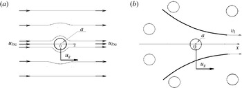
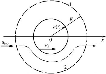
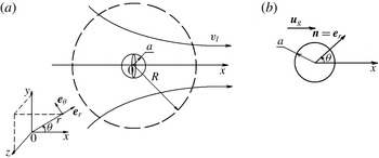
The scheme of the classic statement of the problem of a single particle overflowing by a forward flow is shown in figure 7(a). The force acting on a representative particle in an inviscid incompressible flow is (Lamb Reference Lamb1957)
 $$\begin{eqnarray}f_{bl}=\unicode[STIX]{x1D70C}_{l}\frac{4\unicode[STIX]{x03C0}a^{3}}{3}\frac{\text{d}u_{l\infty }}{\text{d}t}-\unicode[STIX]{x1D70C}_{l}\frac{2\unicode[STIX]{x03C0}a^{3}}{3}\frac{\text{d}(u_{g}-u_{l\infty })}{\text{d}t}=f_{b}+f_{vm}.\end{eqnarray}$$
Here,
 $u_{l\infty }(t)$
is the velocity of the liquid at distance;
 $u_{g}(t)$
is the velocity of the test particle;
 $\text{d}/\text{d}t$
are ordinary derivatives with respect to time. The terms on the right-hand side are usually grouped into expressions for the forces of buoyancy and virtual mass,
 $f_{b}$
,
 $f_{vm}$
.
In a two-phase medium, the particle velocities vary with space and time:
 $u_{g}(t,x)$
. To apply formula (4.28) obtained for a single particle for a particle in ensemble, the derivatives are to be taken along the trajectory of motion of just this particle:
 $$\begin{eqnarray}\frac{\text{d}u_{g}(t)}{\text{d}t}\rightarrow \frac{\text{D}_{g}u_{g}(t,x)}{\text{D}t}=\frac{\unicode[STIX]{x2202}u_{g}}{\unicode[STIX]{x2202}t}+u_{g}\frac{\unicode[STIX]{x2202}u_{g}}{\unicode[STIX]{x2202}x}.\end{eqnarray}$$
It is shown in appendix B that the liquid velocity at distance
 $u_{l\infty }(t)$
is equal to the average velocity of the liquid in the space surrounding this particle,
 $u_{l}$
. Therefore, the derivatives of the liquid velocity could be taken along the trajectory of particles as well:
 $$\begin{eqnarray}\frac{\text{d}u_{l\infty }(t)}{\text{d}t}\rightarrow \frac{\text{D}_{g}u_{l}(t,x)}{\text{D}t}=\frac{\unicode[STIX]{x2202}u_{l}}{\unicode[STIX]{x2202}t}+u_{g}\frac{\unicode[STIX]{x2202}u_{l}}{\unicode[STIX]{x2202}x}.\end{eqnarray}$$
Thus, the force acting on a particle in a two-phase medium,
 $f_{bl}$
, takes the form
 $$\begin{eqnarray}f_{bl}=f_{b}+f_{vm},\end{eqnarray}$$
 $$\begin{eqnarray}f_{b}=\unicode[STIX]{x1D70C}_{l}\frac{4\unicode[STIX]{x03C0}a^{3}}{3}\frac{\text{D}_{g}u_{l}}{\text{D}t},\quad f_{vm}=-\unicode[STIX]{x1D70C}_{l}\frac{2\unicode[STIX]{x03C0}a^{3}}{3}\frac{\text{D}_{g}(u_{g}-u_{l})}{\text{D}t}.\end{eqnarray}$$
To generalize this expression for the case of particle movement in a viscid fluid, the Stokes force is added to the sum of forces acting on the particle (on the right-hand side of (4.31)). The expression for this force does not contain derivatives and does not affect the characteristics of the model.
 $$\begin{eqnarray}f_{bl}=f_{b}+f_{vm}-\frac{4\unicode[STIX]{x03C0}a^{3}}{3}S(u_{g}-u_{l})=\frac{4\unicode[STIX]{x03C0}a^{3}}{3}\left[\unicode[STIX]{x1D70C}_{l}\frac{\text{D}_{g}u_{l}}{\text{D}t}-\frac{\unicode[STIX]{x1D70C}_{l}}{2}\frac{\text{D}_{g}(u_{g}-u_{l})}{\text{D}t}-S(u_{g}-u_{l})\right],\end{eqnarray}$$
where
 $S$
is the drag force per unit velocity given by (1.10).
The statement of the problem on a particle overflowing by a forward (a) or gradient (b) flow.

From the mass conservation equation for the liquid phase one from (4.10a
) for the flow of an incompressible fluid (
 $\unicode[STIX]{x1D70C}_{l}=\text{const.}$
),
 $$\begin{eqnarray}\frac{\unicode[STIX]{x2202}\unicode[STIX]{x1D6FD}}{\unicode[STIX]{x2202}t}+u_{1}\frac{\unicode[STIX]{x2202}\unicode[STIX]{x1D6FD}}{\unicode[STIX]{x2202}x}=(1-\unicode[STIX]{x1D6FD})\frac{\unicode[STIX]{x2202}u_{l}}{\unicode[STIX]{x2202}x},\end{eqnarray}$$
it follows that the divergence of the average velocity arises due to change in the particle distribution in time and space. On the other hand, the formula for the force of the interphase interaction (4.33) is obtained under the assumption that the divergence is zero since the field of the velocity is symmetrical relative to the particle midsection according to the problem statement (figure 7 a). Therefore, closing expression (4.33) is only valid for the model of a rarefied mixture where the particles do not effect the fluid and formula (4.34) is reduced to
 $$\begin{eqnarray}\frac{\unicode[STIX]{x2202}u_{l}}{\unicode[STIX]{x2202}x}=0.\end{eqnarray}$$
For the model with the mass conservation equation (4.34), it needs the expression for the interphase force that considers the presence of neighbouring particles. To deduce such an expression, one must state the problem so that the gradient of the average micro-flow velocity around a representative particle is equal to
 $\unicode[STIX]{x2202}u_{l}/\unicode[STIX]{x2202}x=0$
in macro-flow.
The scheme of the problem statement of a particle overflowing by a gradient flow is shown in figure 7(b). As a flow of an incompressible fluid can be gradient only due to a change in the particle distribution, this statement considers the interaction of the neighbouring particles (with the same degree of accuracy as the mass equation (4.34) does). Voyinov, Voyinov & Petrov (Reference Voyinov, Voyinov and Petrov1973) solved the problem on a sphere overflowing by a gradient flow. (Since the equations of a multiphase flow model were obtained earlier than the solution of Voyinov et al. (Reference Voyinov, Voyinov and Petrov1973), an analogous solution had been obviously obtained by the authors of the model independently.) In appendix C, we give the solution for a particle of variable radius
 $a(t)$
(which will be required later on). If the radius is constant (
 $a=\text{const.}$
), the expression for the interfacial force has the form
 $$\begin{eqnarray}f_{bl}^{\prime }=f_{b}+f_{vm}-\frac{4\unicode[STIX]{x03C0}a^{3}}{3}S(u_{g}-u_{l})-2\unicode[STIX]{x03C0}a^{3}\unicode[STIX]{x1D70C}_{l}(u_{g}-u_{l})\frac{\unicode[STIX]{x2202}u_{l}}{\unicode[STIX]{x2202}x},\end{eqnarray}$$
where the expressions for the buoyancy force
 $f_{b}$
and virtual mass force
 $f_{vm}$
are given by (4.32). Comparing (4.33) and (4.36), we see that the presence of neighbouring particles results in the appearance of an additional term in the expression for the interphase force. This term can be named as the force of bubble interaction,
 $f_{bb}$
,
 $$\begin{eqnarray}f_{bb}=2\unicode[STIX]{x03C0}a^{3}\unicode[STIX]{x1D70C}_{l}(u_{g}-u_{l})\frac{\unicode[STIX]{x2202}u_{l}}{\unicode[STIX]{x2202}x}.\end{eqnarray}$$
The field of stresses in the ‘gas of disperse particles’,
 $\unicode[STIX]{x1D6F1}(t,x)$
, can be introduced as
 $$\begin{eqnarray}\frac{\unicode[STIX]{x2202}\unicode[STIX]{x1D6F1}}{\unicode[STIX]{x2202}x}=f_{bb}\left/\frac{4}{3}\unicode[STIX]{x03C0}a^{3}\right.,\quad \unicode[STIX]{x1D6F1}=\frac{3}{2}\int \unicode[STIX]{x1D70C}_{l}(u_{g}-u_{l})\,\text{d}u_{l}+\unicode[STIX]{x1D6F7}(t),\end{eqnarray}$$
where
 $\unicode[STIX]{x1D6F7}(t)$
is an indefinite time function.
The expression for the force of interphase interaction (4.36) accounting for the mutual influence of dispersed particles can be rewritten in the form
 $$\begin{eqnarray}f_{bl}^{\prime }=f_{b}+f_{vm}-\frac{4\unicode[STIX]{x03C0}a^{3}}{3}S(u_{g}-u_{l})-f_{bb}=f_{b}^{\prime }+f_{vm}^{\prime }-\frac{4\unicode[STIX]{x03C0}a^{3}}{3}S(u_{g}-u_{l}),\end{eqnarray}$$
 $$\begin{eqnarray}f_{b}=\unicode[STIX]{x1D70C}_{l}\frac{4\unicode[STIX]{x03C0}a^{3}}{3}\frac{\text{D}_{g}u_{l}}{\text{D}t},\quad f_{vm}=-\unicode[STIX]{x1D70C}_{l}\frac{2\unicode[STIX]{x03C0}a^{3}}{3}\frac{\text{D}_{g}(u_{g}-u_{l})}{\text{D}t},\end{eqnarray}$$
 $$\begin{eqnarray}f_{b}^{\prime }=\unicode[STIX]{x1D70C}_{l}\frac{4\unicode[STIX]{x03C0}a^{3}}{3}\frac{\text{D}_{l}u_{l}}{\text{D}t},\quad f_{vm}^{\prime }=-\unicode[STIX]{x1D70C}_{l}\frac{2\unicode[STIX]{x03C0}a^{3}}{3}\left(\frac{\text{D}_{g}u_{g}}{\text{D}t}-\frac{\text{D}_{l}u_{l}}{\text{D}t}\right),\end{eqnarray}$$
where
 $f_{b}$
and
 $f_{vm}$
(4.32) have been obtained from the solution of the problem of a particle overflowing by a forward flow (figure 7
a).
In the form (4.39), the force
 $f_{bb}$
has been ‘divided’ into two components. One forms a part of
 $f_{b}^{\prime }$
and the other is a part of
 $f_{vm}^{\prime }$
. It should be noted that there is an insignificant, at first sight, distinction between the forces
 $f_{b}$
and
 $f_{b}^{\prime }$
, and between
 $f_{vm}$
and
 $f_{vm}^{\prime }$
as well: all of the derivatives are taken along the trajectory of particle movement in the first ones; in the second ones the derivatives of the liquid velocity are taken along the trajectory of the liquid phase movement.
On substituting the expression (4.39) for the interphase interaction force
 $f_{bl}^{\prime }$
into the one-dimensional version of the conservation equations for mass and momentum averaged throughout the volume (Ishii & Hibiki Reference Ishii and Hibiki2006), we obtain
 $$\begin{eqnarray}\frac{\unicode[STIX]{x2202}[\unicode[STIX]{x1D70C}_{l}(1-\unicode[STIX]{x1D6FD})]}{\unicode[STIX]{x2202}t}+\frac{\unicode[STIX]{x2202}[\unicode[STIX]{x1D70C}_{l}(1-\unicode[STIX]{x1D6FD})u_{l}]}{\unicode[STIX]{x2202}x}=0,\quad \frac{\unicode[STIX]{x2202}[\unicode[STIX]{x1D70C}_{g}\unicode[STIX]{x1D6FD}]}{\unicode[STIX]{x2202}t}+\frac{\unicode[STIX]{x2202}[\unicode[STIX]{x1D70C}_{g}\unicode[STIX]{x1D6FD}u_{g}]}{\unicode[STIX]{x2202}x}=0,\end{eqnarray}$$
 $$\begin{eqnarray}\unicode[STIX]{x1D70C}_{l}(1-\unicode[STIX]{x1D6FD})\frac{\text{D}_{l}u_{l}}{\text{D}t}+\frac{\unicode[STIX]{x2202}P}{\unicode[STIX]{x2202}x}=-nf_{bl}^{\prime }-F_{w},\quad \unicode[STIX]{x1D70C}_{g}\unicode[STIX]{x1D6FD}\frac{\text{D}_{g}u_{g}}{\text{D}t}=nf_{bl}^{\prime },\end{eqnarray}$$
 $$\begin{eqnarray}f_{bl}^{\prime }=f_{b}^{\prime }+f_{vm}^{\prime }-\frac{4\unicode[STIX]{x03C0}a^{3}}{3}S(u_{g}-u_{l}),\end{eqnarray}$$
where the expressions for
 $f_{b}^{\prime }$
and
 $f_{vm}^{\prime }$
are given by formulae (4.41);
 $n$
is the number of particles per unit mixture volume.
After substituting expressions (4.44), (4.41) for the interphase interaction force
 $f_{bl}^{\prime }$
into the right-hand sides of the momentum equation (4.43), transferring the buoyancy force
 $f_{b}^{\prime }$
into the left-hand side, we are coming to a ‘classic’ system of equations for a bubbly flow with a ‘symmetrical’ momentum equation (4.10)–(4.15).
Thus, the ‘classic’ model (4.10)–(4.15) considers a mutual influence of dispersed particles (4.18), but for the particles located in an incompressible liquid,
 $\unicode[STIX]{x1D70C}_{l}=\text{const.}$
The model (4.5)–(4.7) is correct for the case of an incompressible carrying phase but is not correct on being generalized to the case of a compressible liquid since the system of equations for a compressible medium is closed by the ratio obtained for an incompressible liquid which supposes the velocity of perturbations spread between particles to be instantaneous. Therein lies the self-contradiction of the model, its defect.
Let us correct the system by replacing the expression for the force of the particle interaction in an incompressible medium by the force in a compressible one,
 $f_{bb}^{\prime \prime }$
. The expression for
 $f_{bb}^{\prime \prime }$
is taken in a relaxation approximation,
 $$\begin{eqnarray}f_{bb}^{\prime \prime }={\textstyle \frac{4}{3}}\unicode[STIX]{x03C0}a^{3}\unicode[STIX]{x1D6F1}_{x},\end{eqnarray}$$
 $$\begin{eqnarray}\frac{\text{D}_{g}\unicode[STIX]{x1D6F1}_{x}}{\text{D}t}=\frac{1}{\unicode[STIX]{x1D70F}^{\ast }}\left\{\frac{3}{2}\unicode[STIX]{x1D70C}_{l}(u_{g}-u_{l})\frac{\unicode[STIX]{x2202}u_{l}}{\unicode[STIX]{x2202}x}-\unicode[STIX]{x1D6F1}_{x}\right\},\quad \unicode[STIX]{x1D70F}^{\ast }=\frac{a}{a_{l}\unicode[STIX]{x1D6FD}^{1/3}}.\end{eqnarray}$$
Here,
 $\unicode[STIX]{x1D6F1}_{x}=\unicode[STIX]{x2202}\unicode[STIX]{x1D6F1}/\unicode[STIX]{x2202}x$
is the pressure gradient in the dispersed particle medium;
 $\unicode[STIX]{x1D70F}^{\ast }$
is the time within which the gradient flow is settled around the test particle, i.e. the time necessary for the wave to run the distance between the particles;
 $a/\unicode[STIX]{x1D6FD}^{1/3}$
is the distance between the bubbles;
 $a_{l}$
is the speed of sound in liquid.
On replacing
 $f_{bl}^{\prime }$
by
 $f_{bl}^{\prime \prime }$
in the momentum equations (4.43), we obtain the following system of equations:
 $$\begin{eqnarray}\frac{\unicode[STIX]{x2202}[\unicode[STIX]{x1D70C}_{l}(1-\unicode[STIX]{x1D6FD})]}{\unicode[STIX]{x2202}t}+\frac{\unicode[STIX]{x2202}[\unicode[STIX]{x1D70C}_{l}(1-\unicode[STIX]{x1D6FD})u_{l}]}{\unicode[STIX]{x2202}x}=0,\quad \frac{\unicode[STIX]{x2202}[\unicode[STIX]{x1D70C}_{g}\unicode[STIX]{x1D6FD}]}{\unicode[STIX]{x2202}t}+\frac{\unicode[STIX]{x2202}[\unicode[STIX]{x1D70C}_{g}\unicode[STIX]{x1D6FD}u_{g}]}{\unicode[STIX]{x2202}x}=0,\end{eqnarray}$$
 $$\begin{eqnarray}\unicode[STIX]{x1D70C}_{l}(1-\unicode[STIX]{x1D6FD})\frac{\text{D}_{l}u_{l}}{\text{D}t}+\frac{\unicode[STIX]{x2202}P}{\unicode[STIX]{x2202}x}=-nf_{bl}^{\prime \prime }-F_{w},\quad \unicode[STIX]{x1D70C}_{g}\unicode[STIX]{x1D6FD}\frac{\text{D}_{g}u_{g}}{\text{D}t}=nf_{bl}^{\prime \prime },\end{eqnarray}$$
 $$\begin{eqnarray}f_{bl}^{\prime \prime }=f_{b}+f_{vm}-\frac{4\unicode[STIX]{x03C0}a^{3}}{3}S(u_{g}-u_{l})-\frac{4\unicode[STIX]{x03C0}a^{3}}{3}\unicode[STIX]{x1D6F1}_{x},\end{eqnarray}$$
 $$\begin{eqnarray}f_{b}=\unicode[STIX]{x1D70C}_{l}\frac{4\unicode[STIX]{x03C0}a^{3}}{3}\frac{\text{D}_{g}u_{l}}{\text{D}t},\quad f_{vm}=-\unicode[STIX]{x1D70C}_{l}\frac{2\unicode[STIX]{x03C0}a^{3}}{3}\frac{\text{D}_{g}(u_{g}-u_{l})}{\text{D}t},\end{eqnarray}$$
 $$\begin{eqnarray}\frac{\text{D}_{g}\unicode[STIX]{x1D6F1}_{x}}{\text{D}t}=\frac{1}{\unicode[STIX]{x1D70F}^{\ast }}\left\{\frac{3}{2}\unicode[STIX]{x1D70C}_{l}(u_{g}-u)\frac{\unicode[STIX]{x2202}u}{\unicode[STIX]{x2202}x}-\unicode[STIX]{x1D6F1}_{x}\right\}.\end{eqnarray}$$
The model (4.47)–(4.51) has five real mathematical characteristics in the whole range of volumetric contents. For the first couple, exact analytical expressions are found:
 $$\begin{eqnarray}\left(\frac{\text{d}x}{\text{d}t}\right)_{1,2}=u_{g},\end{eqnarray}$$
and the other three characteristics are determined from the solution of the cubic equation:
 $$\begin{eqnarray}\left.\begin{array}{@{}c@{}}y^{3}-(1+K){\displaystyle \frac{\unicode[STIX]{x0394}u}{a_{l}}}y^{2}+\left(\!K\left(\!{\displaystyle \frac{\unicode[STIX]{x0394}u}{a_{l}}}\right)^{2}-{\displaystyle \frac{(1+2\unicode[STIX]{x1D6FD})\unicode[STIX]{x1D70C}_{l}+2(1-\unicode[STIX]{x1D6FD})\unicode[STIX]{x1D70C}_{g}}{(1-\unicode[STIX]{x1D6FD})((1-\unicode[STIX]{x1D6FD})\unicode[STIX]{x1D70C}_{l}+(2+\unicode[STIX]{x1D6FD})\unicode[STIX]{x1D70C}_{g})}}\!\right)y+k{\displaystyle \frac{\unicode[STIX]{x0394}u}{a_{l}}}=0,\\ K={\displaystyle \frac{3\unicode[STIX]{x1D6FD}\unicode[STIX]{x1D70C}_{g}}{(1-\unicode[STIX]{x1D6FD})\unicode[STIX]{x1D70C}_{l}+(2+\unicode[STIX]{x1D6FD})\unicode[STIX]{x1D70C}_{g}}},\end{array}\right\}\end{eqnarray}$$
where the parameters
 $y$
and
 $k$
are determined by (4.17).
Searching for the roots of (4.53) in the form of the expansion in a small parameter
 $\unicode[STIX]{x1D700}=\unicode[STIX]{x0394}u/a_{l}\ll 1$
, we obtain
 $$\begin{eqnarray}\displaystyle & \displaystyle \left(\frac{\text{d}x}{\text{d}t}\right)_{3}=\frac{3\unicode[STIX]{x1D6FD}\unicode[STIX]{x1D70C}_{l}u_{l}+(1-\unicode[STIX]{x1D6FD})(\unicode[STIX]{x1D70C}_{l}+2\unicode[STIX]{x1D70C}_{g})u_{g}}{(1+2\unicode[STIX]{x1D6FD})\unicode[STIX]{x1D70C}_{l}+2(1-\unicode[STIX]{x1D6FD})\unicode[STIX]{x1D70C}_{g}}+O(\unicode[STIX]{x1D700}^{2}\unicode[STIX]{x0394}u), & \displaystyle\end{eqnarray}$$
 $$\begin{eqnarray}\displaystyle & \displaystyle \left(\frac{\text{d}x}{\text{d}t}\right)_{4,5}=u_{l}\pm a_{l}\sqrt{\frac{(1+2\unicode[STIX]{x1D6FD})\unicode[STIX]{x1D70C}_{l}+2(1-\unicode[STIX]{x1D6FD})\unicode[STIX]{x1D70C}_{g}}{(1-\unicode[STIX]{x1D6FD})((1-\unicode[STIX]{x1D6FD})\unicode[STIX]{x1D70C}_{l}+(2+\unicode[STIX]{x1D6FD})\unicode[STIX]{x1D70C}_{g})}}+O(\unicode[STIX]{x0394}u). & \displaystyle\end{eqnarray}$$
Thus, the model corrected for a compressible fluid with particles of constant radius (4.47)–(4.51) is hyperbolic in the whole range of parameters.
In spite of the fact that the time of installation of a stationary gradient around a disperse particle
 $\unicode[STIX]{x1D70F}^{\ast }$
is negligibly small and much less compared with the characteristic times of any problem, these small corrections inserted into the classic model can change the solutions qualitatively. Critical regimes can be realized in stationary flows under a third characteristic becoming equal to zero. Moreover, waves spreading with the velocity of the third characteristic can be formed during transient processes. Let us give some examples of such flows.
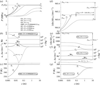
4.7 Simulation with a hyperbolic model of a two-velocity steady-state flow in a diffuser
Let us consider a flow in which calculations with a ‘classic’ model were followed by ‘numerical instabilities’ in solutions (Lahey et al. Reference Lahey, Cheng, Drew and Flaherty1980). For a channel with a variable cross-section, the stationary version of the improved model (4.47)–(4.51) taking into account gravity and neglecting the drag force between the channel walls and flow is
 $$\begin{eqnarray}G_{l}=\unicode[STIX]{x1D70C}_{l}(1-\unicode[STIX]{x1D6FD})u_{l}F=\text{const.},\quad Q_{g}=\unicode[STIX]{x1D6FD}u_{g}F=\text{const.},\end{eqnarray}$$
 $$\begin{eqnarray}\unicode[STIX]{x1D70C}_{l}(1-\unicode[STIX]{x1D6FD})\unicode[STIX]{x1D714}\frac{\text{d}u_{l}}{\text{d}z}+(1-\unicode[STIX]{x1D6FD})\frac{\text{d}P}{\text{d}z}=M_{l}-\unicode[STIX]{x1D70C}_{l}(1-\unicode[STIX]{x1D6FD})g,\quad \unicode[STIX]{x1D714}=(1-\unicode[STIX]{x1D6FD})u_{l}+\unicode[STIX]{x1D6FD}u_{g},\end{eqnarray}$$
 $$\begin{eqnarray}\unicode[STIX]{x1D70C}_{g}\unicode[STIX]{x1D6FD}\unicode[STIX]{x1D714}\frac{\text{d}u_{g}}{\text{d}z}+\unicode[STIX]{x1D6FD}\frac{\text{d}P}{\text{d}z}=\frac{u_{l}}{u_{g}}M_{g}-[\unicode[STIX]{x1D70C}_{l}(1-\unicode[STIX]{x1D6FD})(u_{g}-u_{l})+\unicode[STIX]{x1D70C}_{g}\unicode[STIX]{x1D714}]\frac{\unicode[STIX]{x1D6FD}g}{u_{g}},\end{eqnarray}$$
 $$\begin{eqnarray}\frac{\text{d}\unicode[STIX]{x1D6F1}_{z}}{\text{d}z}=\frac{1}{\unicode[STIX]{x1D70F}^{\ast }u_{g}}\left\{\frac{3}{2}\unicode[STIX]{x1D70C}_{l}(u_{g}-u_{l})\frac{\text{d}u_{l}}{\text{d}z}-\unicode[STIX]{x1D6F1}_{z}\right\},\quad \unicode[STIX]{x1D70F}^{\ast }=\frac{a}{a_{l}\unicode[STIX]{x1D6FD}^{1/3}},\quad a_{l}=\frac{\unicode[STIX]{x1D6FD}_{l}}{\unicode[STIX]{x1D70C}_{l}},\end{eqnarray}$$
 $$\begin{eqnarray}\left.\begin{array}{@{}c@{}}M_{g}=-M_{l}=n(1-\unicode[STIX]{x1D6FD})f_{vm}-\unicode[STIX]{x1D6FD}(1-\unicode[STIX]{x1D6FD})S(u_{g}-u_{l})-\unicode[STIX]{x1D6FD}(1-\unicode[STIX]{x1D6FD})\unicode[STIX]{x1D6F1}_{z},\\ f_{vm}=-\unicode[STIX]{x1D70C}_{l}{\displaystyle \frac{2\unicode[STIX]{x03C0}a^{3}}{3}}u_{g}{\displaystyle \frac{\text{d}(u_{g}-u_{l})}{\text{d}z}},\end{array}\right\}\end{eqnarray}$$
 $$\begin{eqnarray}c_{\unicode[STIX]{x1D707}}=\left\{\begin{array}{@{}ll@{}}24Re^{-1},\quad & Re\leqslant 0.1,\\ 26.33765Re^{-0.8893+0.03417\ln Re+0.001443(\ln Re)^{2}},\quad & Re>0.1,\end{array}\right.\quad Re=2a\unicode[STIX]{x1D70C}_{l}\frac{|u_{g}-u_{l}|}{\unicode[STIX]{x1D707}_{l}},\end{eqnarray}$$
where
 $F$
is the cross-sectional channel area;
 $\unicode[STIX]{x1D714}$
is the volume-average velocity of the mixture;
 $g$
is the acceleration due to gravity;
 $a_{l}$
is the speed of sound in the liquid;
 $S$
is the drag force per unit velocity given by (1.10);
 $C_{\unicode[STIX]{x1D707}}$
is the drag coefficient between a solid particle and fluid taken from Lahey et al. (Reference Lahey, Cheng, Drew and Flaherty1980). The liquid is compressible with the linear equation of state (4.13).
Equations (4.57)–(4.59) in a form suitable for numerical integrating are
 $$\begin{eqnarray}\frac{\text{d}\unicode[STIX]{x1D6FD}}{\text{d}z}=\frac{\text{C}_{2}-\text{C}_{1}}{\text{B}_{2}-\text{B}_{1}},\quad \frac{\text{d}P}{\text{d}z}=\frac{\text{C}_{1}\text{B}_{2}-\text{C}_{2}\text{B}_{1}}{\text{B}_{2}-\text{B}_{1}},\end{eqnarray}$$
 $$\begin{eqnarray}\frac{\text{d}\unicode[STIX]{x1D6F1}_{z}}{\text{d}z}=\frac{1}{\unicode[STIX]{x1D70F}^{\ast }u_{g}}\left\{\frac{3}{2}\unicode[STIX]{x1D70C}_{l}\unicode[STIX]{x0394}uu_{l}\left[-\frac{1}{\unicode[STIX]{x1D70C}_{l}a_{l}^{2}}\frac{\text{d}P}{\text{d}z}+\frac{1}{1-\unicode[STIX]{x1D6FD}}\frac{\text{d}\unicode[STIX]{x1D6FD}}{\text{d}z}-\frac{\text{d}F}{F\text{d}z}\right]-\unicode[STIX]{x1D6F1}_{z}\right\},\end{eqnarray}$$
 $$\begin{eqnarray}\text{B}_{1}={\displaystyle \frac{\unicode[STIX]{x1D70C}_{l}}{2}}{\displaystyle \frac{2u_{l}^{2}+3{\displaystyle \frac{\unicode[STIX]{x1D6FD}}{1-\unicode[STIX]{x1D6FD}}}u_{l}u_{g}+u_{g}^{2}}{1-\left[(1-\unicode[STIX]{x1D6FD})u_{l}+{\displaystyle \frac{3}{2}}\unicode[STIX]{x1D6FD}u_{g}\right]{\displaystyle \frac{u_{l}}{a_{l}^{2}}}}},\quad \text{B}_{2}=-{\displaystyle \frac{\unicode[STIX]{x1D70C}_{l}}{2}}{\displaystyle \frac{u_{l}^{2}+{\displaystyle \frac{1-\unicode[STIX]{x1D6FD}}{\unicode[STIX]{x1D6FD}}}\left(1+{\displaystyle \frac{2\unicode[STIX]{x1D70C}_{g}}{\unicode[STIX]{x1D70C}_{l}}}\right)u_{l}u_{g}+{\displaystyle \frac{2\unicode[STIX]{x1D70C}_{g}}{\unicode[STIX]{x1D70C}_{l}}}u_{g}^{2}}{1+{\displaystyle \frac{1-\unicode[STIX]{x1D6FD}}{2}}{\displaystyle \frac{u_{l}^{2}}{a_{l}^{2}}}}},\end{eqnarray}$$
 $$\begin{eqnarray}\text{C}_{1}=\frac{\unicode[STIX]{x1D70C}_{l}}{2}\frac{2(1-\unicode[STIX]{x1D6FD})u_{l}^{2}+3\unicode[STIX]{x1D6FD}u_{l}u_{g}-\unicode[STIX]{x1D6FD}u_{g}^{2}}{1-\left[(1-\unicode[STIX]{x1D6FD})u_{l}+{\displaystyle \frac{3}{2}}\unicode[STIX]{x1D6FD}u_{g}\right]{\displaystyle \frac{u_{l}}{a_{l}^{2}}}}\frac{\text{d}F}{F\text{d}z}+\frac{\unicode[STIX]{x1D6FD}[S\unicode[STIX]{x0394}u+\unicode[STIX]{x1D6F1}_{z}]-\unicode[STIX]{x1D70C}_{l}g}{1-\left[(1-\unicode[STIX]{x1D6FD})u_{l}+{\displaystyle \frac{3}{2}}\unicode[STIX]{x1D6FD}u_{g}\right]{\displaystyle \frac{u_{l}}{a_{l}^{2}}}},\end{eqnarray}$$
 $$\begin{eqnarray}\displaystyle \text{C}_{2} & = & \displaystyle -\frac{\unicode[STIX]{x1D70C}_{l}}{2}\frac{2(1-\unicode[STIX]{x1D6FD})u_{l}^{2}-(1-\unicode[STIX]{x1D6FD})\left(1+{\displaystyle \frac{2\unicode[STIX]{x1D70C}_{g}}{\unicode[STIX]{x1D70C}_{l}}}\right)u_{l}u_{g}-\unicode[STIX]{x1D6FD}{\displaystyle \frac{2\unicode[STIX]{x1D70C}_{g}}{\unicode[STIX]{x1D70C}_{l}}}u_{g}^{2}}{1+{\displaystyle \frac{1-\unicode[STIX]{x1D6FD}}{2}}{\displaystyle \frac{u_{l}^{2}}{a_{l}^{2}}}}\frac{\text{d}F}{F\text{d}z}\nonumber\\ \displaystyle & & \displaystyle -\,\frac{{\displaystyle \frac{u_{l}}{u_{g}}}(1-\unicode[STIX]{x1D6FD})[S\unicode[STIX]{x0394}u+\unicode[STIX]{x1D6F1}_{z}]+[\unicode[STIX]{x1D70C}_{l}(1-\unicode[STIX]{x1D6FD})\unicode[STIX]{x0394}u+\unicode[STIX]{x1D70C}_{g}\unicode[STIX]{x1D714}]g}{1+{\displaystyle \frac{1-\unicode[STIX]{x1D6FD}}{2}}{\displaystyle \frac{u_{l}^{2}}{a_{l}^{2}}}},\end{eqnarray}$$
where
 $\unicode[STIX]{x0394}u=u_{g}-u_{l}$
is the difference in phase velocities.
Let lightweight particles,
 $\unicode[STIX]{x1D70C}_{g}=1~\text{kg}~\text{m}^{-3}$
, of a constant radius
 $a=0.15~\text{cm}$
be injected with velocity
 $u_{g0}=0.048~\text{m}~\text{s}^{-1}$
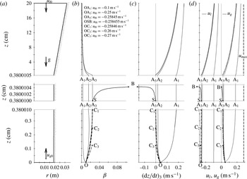
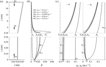
into the narrow bottom end of the diffuser (figure 8
a). The volumetric rate of the particles is
 $Q_{g}=\unicode[STIX]{x1D6FD}_{0}u_{g0}F_{0}=0.547\times 10^{-6}~\text{m}^{3}~\text{s}^{-1}$
(
 $\unicode[STIX]{x1D6FD}_{0}=0.01$
). Water is flowing in the opposite direction (downward). The pressure at a bottom nozzle section is equal to atmospheric pressure.
Figure 8(b–d) shows the solutions obtained under different values of the fluid velocity at the bottom cross-section,
 $u_{l0}$
. Among the solutions obtained, there are continuous,
 $\text{OA}_{1}$
,
 $\text{OA}_{2}$
,
 $\text{OA}_{3}$
, and broken-off, OSB,
 $\text{OC}_{1}$
,
 $\text{OC}_{2}$
,
 $\text{OC}_{3}$
, ones. In continuous regimes, which are realized under small liquid velocity,
 $-0.25\,845~\text{m}~\text{s}^{-1}<u_{l0}<0$
, the particles rising in a downward liquid flow (
 $u_{g}>0$
,
 $u_{l}<0$
) reach the top of the channel (figure 8
d). In these regimes, the liquid velocity decreases in absolute value and the velocity of particles increases, tending to the velocity of a single particle floating up in an infinite volume of a viscous motionless liquid,
 $u_{max}$
, along the nozzle height.
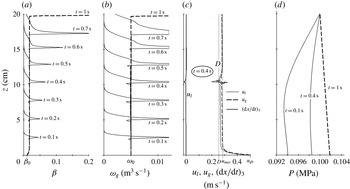
The flow in the diffuser in the frame of a hyperbolic model. (a) The channel geometry. (b–d) The profiles of (b) the volumetric particle content, (c) the third (mass) characteristic, and (d) the liquid and particle velocities. Here,
 $u_{max}$
is the velocity of a single particle floating up in an infinite volume of liquid.

Under liquid velocities
 $u_{l0}\leqslant -0.25\,846~\text{m}~\text{s}^{-1}$
, the parameter gradients exceed the limiting value and the solutions break off (points C
 $_{1}$
–C
 $_{3}$
). Let us write the equation for
 $\text{d}\unicode[STIX]{x1D6FD}/\text{d}z$
(4.62a
) substituting coefficients B
 $_{1}$
, B
 $_{2}$
, C
 $_{1}$
, C
 $_{2}$
(4.64)–(4.66) in it:
 $$\begin{eqnarray}\displaystyle \frac{\text{d}\unicode[STIX]{x1D6FD}}{\text{d}z} & = & \displaystyle \unicode[STIX]{x1D6FD}(1-\unicode[STIX]{x1D6FD})\frac{u_{g}[3\unicode[STIX]{x1D70C}_{l}u_{l}-(\unicode[STIX]{x1D70C}_{l}-\unicode[STIX]{x1D70C}_{g})u_{g}]{\displaystyle \frac{\text{d}F}{F\text{d}z}}+2[S\unicode[STIX]{x0394}u+\unicode[STIX]{x1D6F1}_{z}-(\unicode[STIX]{x1D70C}_{l}-\unicode[STIX]{x1D70C}_{g})g]}{u_{g}[3\unicode[STIX]{x1D6FD}\unicode[STIX]{x1D70C}_{l}u_{l}+(1-\unicode[STIX]{x1D6FD})(\unicode[STIX]{x1D70C}_{l}+2\unicode[STIX]{x1D70C}_{g})u_{g}]}\nonumber\\ \displaystyle & & \displaystyle \times \,\left(1+O\left(\frac{u_{l}^{2}}{a_{l}^{2}}\right)+O\left(\frac{u_{l}u_{g}}{a_{l}^{2}}\right)+O\left(\frac{u_{g}^{2}}{a_{l}^{2}}\right)\right).\end{eqnarray}$$
From (4.67), it is seen that
 $\text{d}\unicode[STIX]{x1D6FD}/\text{d}z\rightarrow \infty$
if the denominator of the equation on the right-hand side is tending to zero.
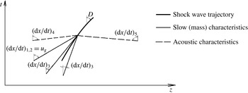
Let us note that the expression in square brackets of the denominator in (4.67) is the numerator of (4.54), which is the equation for the third (mass) characteristic. The bound between the gradients tending to infinity and the characteristic
 $(\text{d}z/\text{d}t)_{3}$
approaching zero is clearly demonstrated by comparison of panels (b) and (c) of figure 8.
The series of solutions turning from a hidden line to the right (
 $\text{OA}_{1}$
–
 $\text{OA}_{3}$
) and left (
 $\text{OC}_{1}$
–
 $\text{OC}_{3}$
) point out that the line is a separatrix with a saddle singular point ‘S’ in it. There is a unique solution OSB with flow transition from a ‘supercritical’ to a ‘subcritical’ one. (Using the terms of gas dynamics, it can be said that the continuous regimes
 $\text{OA}_{1}$
are ‘supercritical’ ones, since the characteristic
 $(\text{d}z/\text{d}t)_{3}$
is always positive (figure 8
c).) The separatrix OSB cannot be obtained by a fourth integration of the system of ordinary differential equations (4.62) since it is not possible to guess an exact, with an infinite number of characters after the point, value of the liquid velocity
 $u_{l0}$
. At the slightest deviation from this exact value, the solution turns either left, as
 $\text{OA}_{1}$
do, or right, like
 $\text{OC}_{1}$
do (figure 8
b). To obtain the separatrix OSB, a special numerical method was required.
In a subcritical sector of the separatrix, SB, quick compaction of particles occurs. At that point, the absolute value of the negative stress gradient in the dispersed particle medium
 $\unicode[STIX]{x1D6F1}_{z}$
increases sharply;
 $\text{d}\unicode[STIX]{x1D6FD}/\text{d}z\rightarrow \infty$
(4.67), and the separatrix ‘breaks off’ (point B). The effect of the increase in the absolute value of
 $\unicode[STIX]{x1D6F1}_{z}$
with particle content
 $\unicode[STIX]{x1D6FD}$
increasing follows from (4.59), (4.67). The increase in
 $\unicode[STIX]{x1D6FD}$
results in the liquid velocity decreasing (4.56a
), which, according to (4.59), causes a subsequent increase in the absolute value of
 $\unicode[STIX]{x1D6F1}_{z}$
, which, since the regime is ‘subcritical’ and the denominator in (4.67) is negative, leads to the increase in the particle content
 $\unicode[STIX]{x1D6FD}$
. The rate of changing
 $\unicode[STIX]{x1D6FD}$
and the other parameters in the subcritical sector of the separatrix SB is determined by the value of
 $\unicode[STIX]{x1D70F}^{\ast }$
(the time within which a gradient flow is settled around a particle).
Thus, the calculations of liquid–particle countercurrent flow with a hyperbolic version of the ‘dirty water’ model (4.47)–(4.51) have shown the existence of a limiting regime
 $\text{OA}_{3}$
with a maximum by absolute value of liquid velocity,
 $u_{l0}\approx -0.25\,845~\text{m}~\text{s}^{-1}$
, for which a continuous solution with the particles rising up to the top nozzle section can be obtained.
4.8 The comparison of calculations with a hyperbolic and ‘classic’ model
A stationary version of the ‘classic’ model (22)–(27) of Lahey et al. (Reference Lahey, Cheng, Drew and Flaherty1980), taking into account gravity and neglecting the liquid compressibility (
 $\unicode[STIX]{x1D70C}_{l}=\text{const.}$
) and the drag force between the channel walls and the fluid
 $F_{w}$
, for a channel of variable cross-section is
 $$\begin{eqnarray}Q_{l}=(1-\unicode[STIX]{x1D6FD})u_{l}F=\text{const.},\quad Q_{g}=\unicode[STIX]{x1D6FD}u_{g}F=\text{const.},\end{eqnarray}$$
 $$\begin{eqnarray}\unicode[STIX]{x1D70C}_{l}(1-\unicode[STIX]{x1D6FD})u_{l}\frac{\text{d}u_{l}}{\text{d}z}+(1-\unicode[STIX]{x1D6FD})\frac{\text{d}P}{\text{d}z}=M_{l}-\unicode[STIX]{x1D70C}_{l}(1-\unicode[STIX]{x1D6FD})g,\quad \unicode[STIX]{x1D70C}_{g}\unicode[STIX]{x1D6FD}u_{g}\frac{\text{d}u_{l}}{\text{d}z}+\unicode[STIX]{x1D6FD}\frac{\text{d}P}{\text{d}z}=M_{g}-\unicode[STIX]{x1D70C}_{g}\unicode[STIX]{x1D6FD}g,\end{eqnarray}$$
 $$\begin{eqnarray}M_{g}=-M_{l}=n(1-\unicode[STIX]{x1D6FD})f_{vm}^{\prime }-\unicode[STIX]{x1D6FD}(1-\unicode[STIX]{x1D6FD})S(u_{g}-u_{l}),\quad f_{vm}^{\prime }=-\unicode[STIX]{x1D70C}_{l}\frac{2\unicode[STIX]{x03C0}a^{3}}{3}\left(u_{g}\frac{\text{d}u_{g}}{\text{d}z}-u_{l}\frac{\text{d}u_{l}}{\text{d}z}\right).\end{eqnarray}$$
After transformations, we obtain equations of the same form as (4.62), but with other expressions for B
 $_{1}$
, B
 $_{2}$
, C
 $_{1}$
and C
 $_{2}$
which do not contain the pressure due to neglect of liquid compressibility. Therefore, the volumetric particle contents and phase velocities can be calculated with the help of only (4.62a
), which, after substituting B
 $_{1}$
, B
 $_{2}$
, C
 $_{1}$
and C
 $_{2}$
, takes the form
 $$\begin{eqnarray}\frac{\text{d}\unicode[STIX]{x1D6FD}}{\text{d}z}=\unicode[STIX]{x1D6FD}(1-\unicode[STIX]{x1D6FD})\frac{[3\unicode[STIX]{x1D70C}_{l}u_{l}^{2}-(\unicode[STIX]{x1D70C}_{l}+2\unicode[STIX]{x1D70C}_{g})u_{g}^{2}]{\displaystyle \frac{\text{d}F}{F\text{d}z}}+2[S\unicode[STIX]{x0394}u-(\unicode[STIX]{x1D70C}_{l}-\unicode[STIX]{x1D70C}_{g})g]}{3\unicode[STIX]{x1D6FD}\unicode[STIX]{x1D70C}_{l}u_{l}^{2}+(1-\unicode[STIX]{x1D6FD})(\unicode[STIX]{x1D70C}_{l}+2\unicode[STIX]{x1D70C}_{g})u_{g}^{2}}.\end{eqnarray}$$
The denominator of (4.71) vanishes only at a stagnation point,
 $u_{g}=u_{l}=0$
, and, therefore, discontinuous solutions are not possible.
Figure 9 compares calculations of the flow in the diffuser with the improved and classic models. For the continuous regimes
 $\text{OA}_{1}$
–
 $\text{OA}_{3}$
, the calculations do not differ. The discontinuous solutions
 $\text{OC}_{2}$
and
 $\text{OC}_{3}$
coincide up to the points of break off (C
 $_{2}$
, C
 $_{3}$
). However, the classic model builds the solutions further.
Thus, the classic model rejects the existence of the limit regime
 $\text{OA}_{3}$
predicted by the hyperbolic model. ‘Numerical instabilities’ of solutions of the classic model can be due to solution bifurcation in the vicinity of a saddle singular point indefinable by this model.
The flow in a diffuser in the frame of the ‘classic’ and hyperbolic models. (a) The channel geometry. (b,c) The profiles of (b) the volumetric particle content, (c) the liquid and particle velocities. Here,
 $u_{max}$
is the velocity of a single particle floating up in an infinite volume of liquid.

4.9 Superslow ‘creeping’ shock waves in a two-phase two-velocity medium
Consider a transient upward flow of solid particles. A cylindrical vessel of 20 cm height is occupied with water (figure 10
a). At
 $t=0$
, solid particles of radius
 $a=0.15~\text{cm}$
start being injected from the bottom of the tube with velocity
 $u_{g0}$
. The liquid velocity at the bottom is zero,
 $u_{l0}=0$
. The pressure at the top tube cross-section is equal to atmospheric pressure.
Let us consider the flow in the frame of the hyperbolic ‘dirty water’ model (4.47)–(4.51), in which the force of gravitation is additionally considered and the flow wall friction is neglected. Then, equations (4.48)–(4.50) take the form
 $$\begin{eqnarray}\unicode[STIX]{x1D70C}_{l}(1-\unicode[STIX]{x1D6FD})\frac{\text{D}_{l}u_{l}}{\text{D}t}+\frac{\unicode[STIX]{x2202}P}{\unicode[STIX]{x2202}x}=-nf_{bl}^{\prime \prime }-\unicode[STIX]{x1D70C}_{l}(1-\unicode[STIX]{x1D6FD})g,\quad \unicode[STIX]{x1D70C}_{g}\unicode[STIX]{x1D6FD}\frac{\text{D}_{g}u_{g}}{\text{D}t}=nf_{bl}^{\prime \prime }-\unicode[STIX]{x1D70C}_{g}\unicode[STIX]{x1D6FD}g,\end{eqnarray}$$
 $$\begin{eqnarray}f_{bl}^{\prime \prime }=\unicode[STIX]{x1D70C}_{l}\frac{4\unicode[STIX]{x03C0}a^{3}}{3}\frac{\text{D}_{g}u_{l}}{\text{D}t}-\unicode[STIX]{x1D70C}_{l}\frac{2\unicode[STIX]{x03C0}a^{3}}{3}\frac{\text{D}_{g}(u_{g}-u_{l})}{\text{D}t}-\frac{4\unicode[STIX]{x03C0}a^{3}}{3}S(u_{g}-u_{l})-\frac{4\unicode[STIX]{x03C0}a^{3}}{3}\unicode[STIX]{x1D6F1}_{z}+\unicode[STIX]{x1D70C}_{l}\frac{4\unicode[STIX]{x03C0}a^{3}}{3}g.\end{eqnarray}$$
For calculations, the ‘double triangle’ numerical method was used, described briefly in § 6, and in appendix B of Ivashnyov et al. (Reference Ivashnyov, Ivashneva and Smirnov2000) in detail.
High-frequency vibrations in an upward flow of solid particles. (a) The flow scheme. (b–e) The oscillograms of (b,c) the pressure, (d) the volumetric particle content and (e) the volumetric mixture flux.

First, we will analyse the case when the particles are injected with a small velocity
 $u_{g0}=1~\text{cm}~\text{s}^{-1}$
. The volumetric rate of the injected particles is
 $\unicode[STIX]{x1D714}_{0}=\unicode[STIX]{x1D6FD}_{0}u_{g0}=10^{-3}~\text{m}^{3}~\text{s}^{-1}$
(
 $\unicode[STIX]{x1D6FD}_{0}=0.1$
).
The particle injection causes waves of two types: fast and slow ones. Figure 10(b–e) shows the evolution of fast waves. The particle injection leads to the formation of a compression wave which propagates up to the vessel top. On reaching it, the wave is reflected from the free surface as a wave of rarefaction and, by the instant
 $t\approx 2H/a_{l}=0.26~\text{ms}$
, returns to the bottom cross-section. On reaching the bottom end, the wave is reflected and goes upward. After reflecting from the open end, it returns into the vessel as a compression wave. As a result, there arise pressure vibrations with period
 $T\approx 4H/a_{l}=0.52~\text{ms}$
(figure 10
b).
As the particles fill up the vessel (figure 10
d), the ‘fork’ ideality is broken and the vibration amplitude decreases gradually (figure 10
b,c). To characterize the intensity of the acoustic vibrations, let us use a relative deviation of the volumetric mixture rate
 $\unicode[STIX]{x1D714}$
. Summing equations (4.47) of the phase continuity rewritten for constant density of the liquid, we obtain the integral
 $$\begin{eqnarray}\unicode[STIX]{x1D714}=(1-\unicode[STIX]{x1D6FD})u_{l}+\unicode[STIX]{x1D6FD}u_{g}=\text{const.}\end{eqnarray}$$
Thus, in the case of fluid component incompressibility, the volumetric mixture rate
 $\unicode[STIX]{x1D714}$
is constant and equal to its value at the entrance,
 $$\begin{eqnarray}\unicode[STIX]{x1D714}=\unicode[STIX]{x1D714}_{0}=10^{-3}~\text{m}~\text{s}^{-1},\end{eqnarray}$$
and therefore the amplitude of vibrations
 $\unicode[STIX]{x1D714}$
characterizes the mixture compressibility. As is seen from figure 10(e), by the time moment
 $t=0.5~\text{s}$
, the change in
 $\unicode[STIX]{x1D714}$
is comparable to its absolute value,
 $|\unicode[STIX]{x0394}\unicode[STIX]{x1D714}|\sim \unicode[STIX]{x1D714}_{0}$
.
The evolution of slow waves in an upward flow of solid particles. (a,b) For seven instants (shown in the plot), the profiles of (a) the particle volumetric content and (b) the particle mass flow rate,
 $\unicode[STIX]{x1D714}_{g}=\unicode[STIX]{x1D6FD}u_{g}$
. (c,d) For
 $t=0.4~\text{s}$
, (c) the velocity profiles of the liquid, particles and third characteristic, and (d) the pressure profile. Here,
 $u_{max}\approx 0.28~\text{m}~\text{s}^{-1}$
is the velocity of a single particle floating up in an infinite volume of liquid.

Simultaneously with the acoustic waves, two slow waves whose velocities are determined by the phase velocities,
 $u_{g}$
and
 $(\text{d}z/\text{d}t)_{3}$
, travel up the vessel. In figure 11(a), a stepwise increase in the volumetric particle content rising to the vessel top is seen. Figure 11(c) shows the profiles of the velocities of the two mass characteristics. These velocities, practically coinciding,
 $u_{g}\approx (\text{d}z/\text{d}t)_{3}$
, decrease along the wave. Since the characteristic velocity decreases, backward perturbations lag behind forward ones and the waves expand (like a rarefaction wave in an ideal gas). Thus, the wave shown in figure 11(a) represents a combination of two expanding waves.
Since both characteristic velocities are positive,
 $u_{g}>0$
,
 $(\text{d}z/\text{d}t)_{3}>0$
, the wave moves only upward and, after its passage, the particle volumetric rate equalizes within the tube height,
 $\unicode[STIX]{x1D714}_{g}=\unicode[STIX]{x1D6FD}u_{g}$
(figure 11
b).
High-frequency oscillations do not have a visible effect on slow-wave evolution, obviously due to the fact that rarefaction and compression quick waves compensate each other’s influence. By the time moment
 $t=0.7~\text{s}$
, when slow waves have reached the upper cross-section, the vibrations caused by the quick-wave propagation attenuate, and a stationary flow satisfying the integral ratio
 $$\begin{eqnarray}\unicode[STIX]{x1D714}=\unicode[STIX]{x1D714}_{g}=\text{const.}\end{eqnarray}$$
is settled.
The upward flow of solid particles in the case when the velocity of particle injection exceeds the velocity of a single particle floating up in an infinite volume of liquid,
 $u_{max}$
(shown in c). (a–b) The profiles of the particle (a) volumetric content and (b) mass flow rate,
 $\unicode[STIX]{x1D714}_{g}=\unicode[STIX]{x1D6FD}u_{g}$
, at different time moments. (c) The velocity profiles of the liquid, particles and the third characteristic at
 $t=0.4~\text{s}$
. (d) The pressure profiles. Here,
 $D$
is the velocity of the shock (second) wave determined as the travelled distance/time ratio.

Let us now analyse the second case, when the particles are injected with a velocity exceeding
 $u_{max}$
, the velocity of a single particle floating up in an infinite volume of liquid,
 $$\begin{eqnarray}u_{g0}=50~\text{cm}~\text{s}^{-1}>u_{max}=28~\text{cm}~\text{s}^{-1}.\end{eqnarray}$$
The volumetric rate of particle injection is
 $\unicode[STIX]{x1D714}_{0}=\unicode[STIX]{x1D6FD}_{0}u_{g0}=0.005~\text{m}^{3}~\text{s}^{-1}$
(
 $\unicode[STIX]{x1D6FD}_{0}=0.01$
).
The profile of volumetric particle content (figure 12 a) shows a peak formed by two slow waves, a ‘plume of particles’ rising up to the vessel top. The profiles of the velocities of the mass invariant spreading are given in figure 12(c). The velocities coincide up to the moment of slow-wave arrival and then separate, decreasing along the first wave and increasing along the second one. Therefore, the first wave expands and the second one steepens, and turns into a shock wave.
Any perturbation spreads with a characteristic velocity. As the velocities of the first two characteristics exceed that of the third one (figure 12 c),
 $$\begin{eqnarray}(\text{d}z/\text{d}t)_{1,2}=u_{g}>(\text{d}z/\text{d}t)_{3},\end{eqnarray}$$
the velocity of the forward going stretching wave is determined by the first characteristic,
 $(\text{d}z/\text{d}t)_{1,2}=u_{g}$
, and the movement of the lagging shock one is defined by the third characteristic,
 $(\text{d}z/\text{d}t)_{3}$
.
The bound between the third characteristic and the shock wave is determined by the condition of jump evolution. Passing on to a moving frame linked with the jump and neglecting the change in the liquid density, we obtain five ratios preserved across the jump:
 $$\begin{eqnarray}\displaystyle & q_{l}=(1-\unicode[STIX]{x1D6FD})v_{l}=\text{const.}, & \displaystyle\end{eqnarray}$$
 $$\begin{eqnarray}\displaystyle & q_{g}=\unicode[STIX]{x1D6FD}v_{g}=\text{const.}, & \displaystyle\end{eqnarray}$$
 $$\begin{eqnarray}\displaystyle & \displaystyle R=q_{l}v_{l}+\frac{P}{\unicode[STIX]{x1D70C}_{l}^{\ast }}+\frac{q_{g}}{2}(3v_{l}-v_{g})=\text{const.}, & \displaystyle\end{eqnarray}$$
 $$\begin{eqnarray}\displaystyle & I=3\unicode[STIX]{x1D70C}_{l}^{\ast }v_{l}-(\unicode[STIX]{x1D70C}_{l}^{\ast }+2\unicode[STIX]{x1D70C}_{g})v_{g}=\text{const.}, & \displaystyle\end{eqnarray}$$
 $$\begin{eqnarray}\displaystyle & \displaystyle \unicode[STIX]{x1D6F1}_{x2}-\unicode[STIX]{x1D6F1}_{x1}=\frac{3\unicode[STIX]{x1D6FD}_{l}q_{l}}{2a}\int _{\unicode[STIX]{x1D6FD}_{1}}^{\unicode[STIX]{x1D6FD}_{2}}\frac{\unicode[STIX]{x1D6FD}^{1/3}}{(1-\unicode[STIX]{x1D6FD})^{2}}\left[1-\frac{\unicode[STIX]{x1D6FD}q_{l}}{(1-\unicode[STIX]{x1D6FD})q_{g}}\right]\text{d}\unicode[STIX]{x1D6FD}, & \displaystyle\end{eqnarray}$$
 $$\begin{eqnarray}\displaystyle & v_{l}=u_{l}-D, & \displaystyle\end{eqnarray}$$
 $$\begin{eqnarray}\displaystyle & v_{g}=u_{g}-D, & \displaystyle\end{eqnarray}$$
where
 $v_{l}$
and
 $v_{g}$
are the liquid and particle velocities in the moving frame;
 $\unicode[STIX]{x1D70C}_{l}^{\ast }=\unicode[STIX]{x1D70C}_{l}(P_{atm})=\text{const.}$
represents the liquid density.
There are 11 unknown parameters in five equations (4.79)–(4.83):
 $\unicode[STIX]{x1D6FD}$
,
 $P$
,
 $v_{l}$
,
 $v_{g}$
,
 $\unicode[STIX]{x1D6F1}_{x}$
are unknown on both sides of the shock wave, and the wave velocity
 $D$
is not known either. Therefore, six additional ratios should be added to the five equations to resolve them. Invariants preserved along five characteristics are such ratios, but since there are only five characteristics, one of them must come to the jump twice: from the fields ahead of and behind it (figure 13). It is this characteristic of coming twice with which the jump is bounded. Then, the jump velocity
 $D$
must satisfy the condition
 $$\begin{eqnarray}[(\text{d}x/\text{d}t)_{3}]_{1}<D<[(\text{d}x/\text{d}t)_{3}]_{2},\end{eqnarray}$$
where
 $[(\text{d}x/\text{d}t)_{3}]_{1}$
and
 $[(\text{d}x/\text{d}t)_{3}]_{2}$
are characteristic velocities before and behind the front of the shock wave.
The bound between characteristics and a shock wave.

Figure 12(c) clearly shows that condition (4.86) is satisfied.
5 The boiling flow model accounting for wall surface nucleation and bubble breakup
5.1 Basic model assumptions
A model of a three-phase medium is suggested. The phases are fluid, immovable
 $\unicode[STIX]{x1D6FC}$
-bubbles growing at walls and
 $\unicode[STIX]{x1D6FD}$
-bubbles moving in the flow (figure 6).
-
(i) Boiling is considered to start at the channel wall surface. The number of centres of nucleation per unit wall surface area
 $N$
is a free model parameter. In the flow volume, boiling centres are initially lacking and appear only after the fragmentation of wall
$\unicode[STIX]{x1D6FC}$
-bubbles.
-
(ii) The fragmentation of both
$\unicode[STIX]{x1D6FC}$
- and
$\unicode[STIX]{x1D6FD}$
-bubbles is induced by Kelvin–Helmholtz instability. The critical value of the Weber number,
$We^{\ast }$
, is the second of two free model parameters. -
(iii) The size and velocity distribution of
$\unicode[STIX]{x1D6FD}$
-bubbles across a channel section is neglected. -
(iv) The
$\unicode[STIX]{x1D6FC}$
-bubbles are assumed to be in the form of a hemisphere and the
$\unicode[STIX]{x1D6FD}$
-bubbles are ball-shaped. (The supposition about regular geometry of the bubbles is used for the interphase drag and heat transfer models.) -
(v) The pressures in the phases are considered to be equal,
$P_{l}=P_{\unicode[STIX]{x1D6FC}}=P_{\unicode[STIX]{x1D6FD}}=P$
.This assumption is accepted on the grounds of the evaluation of the time of pressure equalization between a motionless vapour bubble and the evaporating fluid surrounding it. This process studied using the model for a spherical bubble in an inertial liquid has shown that the pressures in the bubble and liquid equalize within only 2–3 bubble oscillations. (The evaporation is an essential damping factor.) The oscillation period can be evaluated by the formula
(5.1)
$$\begin{eqnarray}\unicode[STIX]{x1D70F}_{b}\sim a\sqrt{\frac{\unicode[STIX]{x1D70C}_{l}}{P}}.\end{eqnarray}$$
The characteristic dimensions of
$\unicode[STIX]{x1D6FC}$
- and
$\unicode[STIX]{x1D6FD}$
-bubbles are determined by the fragmentation process and can be evaluated from the expression for the Weber number (1.8). Assuming that the critical Weber number
$We^{\ast }=1$
, using the evaluation for the flow velocity
$u_{l}^{\ast }\sim 10~\text{m}~\text{s}^{-1}$
(4.1) and accepting the difference in the phase velocities
$\unicode[STIX]{x0394}u_{l}^{\ast }=1~\text{m}~\text{s}^{-1}$
, we can evaluate
$\unicode[STIX]{x1D6FC}$
- and
$\unicode[STIX]{x1D6FD}$
-bubble dimensions as (5.2a,b )
$$\begin{eqnarray}a_{\unicode[STIX]{x1D6FC}}\leqslant \frac{\unicode[STIX]{x1D70E}We^{\ast }}{2\unicode[STIX]{x1D70C}_{g}(u_{l}^{\ast })^{2}}\sim 10^{-6}~\text{m},\quad a_{\unicode[STIX]{x1D6FD}}\leqslant \frac{\unicode[STIX]{x1D70E}We^{\ast }}{2\unicode[STIX]{x1D70C}_{g}(\unicode[STIX]{x0394}u_{l}^{\ast })^{2}}\sim 10^{-4}~\text{m}.\end{eqnarray}$$
Thus, the oscillation period is
$\unicode[STIX]{x1D70F}_{b}\sim 10^{-6}~\text{s}$
even for large
$\unicode[STIX]{x1D6FD}$
-bubbles, that is several orders of magnitude less than the characteristic time of the pressure change in the compression wave, which does not exceed
$\unicode[STIX]{x1D70F}_{P}\sim 10^{-3}~\text{s}$
(figure 1). Since
$\unicode[STIX]{x1D70F}_{b}\ll \unicode[STIX]{x1D70F}_{P}$
, we can neglect the inertia of the liquid surrounding a bubble and adopt the assumption about the equality of the pressures in the phases (v). -
(vi) The parameters in the
$\unicode[STIX]{x1D6FC}$
- and
$\unicode[STIX]{x1D6FD}$
-bubbles are uniform over their radii and equal to the parameters on the line of saturation,
$T_{g}=T_{s}(P)$
,
$\unicode[STIX]{x1D70C}_{g}=\unicode[STIX]{x1D70C}_{gs}(P)$
. -
(vii) The vapour density is much less than the liquid density,
$\unicode[STIX]{x1D70C}_{g}\ll \unicode[STIX]{x1D70C}_{l}$
.From this assumption, the equality of the mean-mass mixture velocity
$u$
and the liquid velocity
$u_{l}$
follows: (5.3)
$$\begin{eqnarray}u=(1-\unicode[STIX]{x1D712})u_{l}+\unicode[STIX]{x1D712}u_{g}\approx u_{l},\quad \unicode[STIX]{x1D712}=\frac{\unicode[STIX]{x1D70C}_{g}\unicode[STIX]{x1D6FD}}{\unicode[STIX]{x1D70C}}.\end{eqnarray}$$
Here,
$\unicode[STIX]{x1D712}$
is the mass fraction of
$\unicode[STIX]{x1D6FD}$
-bubbles in the flow;
$u_{g}$
is the velocity of
$\unicode[STIX]{x1D6FD}$
-bubbles. -
(viii) The velocity of fragments separating from
$\unicode[STIX]{x1D6FC}$
-bubbles is assumed to be zero,
$u_{\unicode[STIX]{x1D6FC}\unicode[STIX]{x1D6FD}}=0$
. (After the separation, the fragments instantly acquire the
$\unicode[STIX]{x1D6FD}$
-vapour velocity (according to assumption (iii)).) The velocity of the liquid vaporizing into
$\unicode[STIX]{x1D6FC}$
- and
$\unicode[STIX]{x1D6FD}$
-bubbles is considered to be equal to the velocity of
$\unicode[STIX]{x1D6FC}$
- and
$\unicode[STIX]{x1D6FD}$
-vapour,
$u_{l\unicode[STIX]{x1D6FC}}=0$
,
$u_{l\unicode[STIX]{x1D6FD}}=u_{g}$
.





5.2 Equations of mass balance
The one-dimensional mass equations for the liquid,
 $\unicode[STIX]{x1D6FC}$
- and
 $\unicode[STIX]{x1D6FD}$
-vapour have the form
 $$\begin{eqnarray}\frac{\unicode[STIX]{x2202}[\unicode[STIX]{x1D70C}_{l}(1-\unicode[STIX]{x1D6FC})(1-\unicode[STIX]{x1D6FD})]}{\unicode[STIX]{x2202}t}+\frac{\unicode[STIX]{x2202}[\unicode[STIX]{x1D70C}_{l}(1-\unicode[STIX]{x1D6FC})(1-\unicode[STIX]{x1D6FD})u]}{\unicode[STIX]{x2202}x}=-J_{l\unicode[STIX]{x1D6FC}}-J_{l\unicode[STIX]{x1D6FD}},\end{eqnarray}$$
 $$\begin{eqnarray}\frac{\unicode[STIX]{x2202}[\unicode[STIX]{x1D70C}_{g}\unicode[STIX]{x1D6FC}]}{\unicode[STIX]{x2202}t}=-J_{\unicode[STIX]{x1D6FC}\unicode[STIX]{x1D6FD}}+J_{l\unicode[STIX]{x1D6FC}},\quad \frac{\unicode[STIX]{x2202}[\unicode[STIX]{x1D70C}_{g}(1-\unicode[STIX]{x1D6FC})\unicode[STIX]{x1D6FD}]}{\unicode[STIX]{x2202}t}+\frac{\unicode[STIX]{x2202}[\unicode[STIX]{x1D70C}_{g}(1-\unicode[STIX]{x1D6FC})\unicode[STIX]{x1D6FD}u_{g}]}{\unicode[STIX]{x2202}x}=J_{\unicode[STIX]{x1D6FC}\unicode[STIX]{x1D6FD}}+J_{l\unicode[STIX]{x1D6FD}}.\end{eqnarray}$$
 $$\begin{eqnarray}\unicode[STIX]{x1D6FC}=\frac{2}{3}\unicode[STIX]{x03C0}a_{\unicode[STIX]{x1D6FC}}^{3}\frac{4N}{D_{ch}},\quad \unicode[STIX]{x1D6FD}=\frac{4}{3}\unicode[STIX]{x03C0}a_{\unicode[STIX]{x1D6FD}}^{3}n,\quad n=\unicode[STIX]{x1D70C}c,\quad \unicode[STIX]{x1D70C}=(1-\unicode[STIX]{x1D6FD})\unicode[STIX]{x1D70C}_{l}+\unicode[STIX]{x1D6FD}\unicode[STIX]{x1D70C}_{g},\end{eqnarray}$$
where
 $\unicode[STIX]{x1D6FC}$
is the volumetric fraction of
 $\unicode[STIX]{x1D6FC}$
-vapour in the whole volume of the three-phase mixture;
 $N=\text{const.}$
is the number of
 $\unicode[STIX]{x1D6FC}$
-bubbles per unit area of the wall surface;
 $D_{ch}$
is the inner diameter of the channel;
 $n$
and
 $c$
are the numbers of
 $\unicode[STIX]{x1D6FD}$
-bubbles per unit volume and mass of the moving mixture (not including
 $\unicode[STIX]{x1D6FC}$
-bubbles);
 $\unicode[STIX]{x1D70C}$
is the density of the moving mixture;
 $J_{l\unicode[STIX]{x1D6FC}}$
and
 $J_{l\unicode[STIX]{x1D6FD}}$
are the liquid masses evaporating into the
 $\unicode[STIX]{x1D6FC}$
- and
 $\unicode[STIX]{x1D6FD}$
-bubbles per unit volume of all the mixture in unit time;
 $J_{\unicode[STIX]{x1D6FC}\unicode[STIX]{x1D6FD}}$
is the mass of
 $\unicode[STIX]{x1D6FC}$
-vapour converted into
 $\unicode[STIX]{x1D6FD}$
-vapour per unit mixture volume in unit time;
 $a_{\unicode[STIX]{x1D6FC}}$
and
 $a_{\unicode[STIX]{x1D6FD}}$
are the radii of
 $\unicode[STIX]{x1D6FC}$
- and
 $\unicode[STIX]{x1D6FD}$
-bubbles.
The intensities of liquid evaporation into
 $\unicode[STIX]{x1D6FC}$
- and
 $\unicode[STIX]{x1D6FD}$
-bubbles are determined by
 $$\begin{eqnarray}J_{l\unicode[STIX]{x1D6FC}}=\frac{4N}{D_{ch}}j_{l\unicode[STIX]{x1D6FC}},\quad J_{l\unicode[STIX]{x1D6FD}}=n(1-\unicode[STIX]{x1D6FC})j_{l\unicode[STIX]{x1D6FD}},\end{eqnarray}$$
 $$\begin{eqnarray}j_{l\unicode[STIX]{x1D6FC}}=\unicode[STIX]{x03C0}D_{ls}a_{\unicode[STIX]{x1D6FC}}\unicode[STIX]{x1D70C}_{g}Ja\,Nu,\quad j_{l\unicode[STIX]{x1D6FD}}=2\unicode[STIX]{x03C0}D_{ls}a_{\unicode[STIX]{x1D6FD}}\unicode[STIX]{x1D70C}_{g}Ja\,Nu,\quad D_{ls}=\unicode[STIX]{x1D706}_{ls}(\unicode[STIX]{x1D70C}_{ls}c_{ls})^{-1},\end{eqnarray}$$
where
 $j_{l\unicode[STIX]{x1D6FC}}$
and
 $j_{l\unicode[STIX]{x1D6FD}}$
are the rates of liquid evaporation into each bubble of the
 $\unicode[STIX]{x1D6FC}$
- and
 $\unicode[STIX]{x1D6FD}$
-phases;
 $\unicode[STIX]{x1D706}_{ls}$
and
 $D_{ls}$
are the coefficients of thermal conductivity and thermal diffusivity of the fluid at the curve of saturation.
The dependence of the dimensionless heat flux into a bubble, the Nusselt number, on the dimensionless liquid overheat,
 $Nu(Ja)$
, is determined from a self-similar solution of the problem of heat bubble growth in a superheated liquid (Scriven Reference Scriven1959) with formula (1.5).
The intensity of the phase transition between the
 $\unicode[STIX]{x1D6FC}$
- and
 $\unicode[STIX]{x1D6FD}$
-vapour bubbly phases is
 $$\begin{eqnarray}J_{\unicode[STIX]{x1D6FC}\unicode[STIX]{x1D6FD}}=\frac{8}{3D_{ch}}\unicode[STIX]{x03C0}a_{\unicode[STIX]{x1D6FC}}^{3}\unicode[STIX]{x1D70C}_{g}\unicode[STIX]{x1D713}_{\unicode[STIX]{x1D6FC}},\end{eqnarray}$$
where
 $\unicode[STIX]{x1D713}_{\unicode[STIX]{x1D6FC}}$
is the intensity of
 $\unicode[STIX]{x1D6FC}$
-bubble breakup: the number of
 $\unicode[STIX]{x1D6FC}$
-bubble fragments passing into the flow from a unit of the wall surface per unit time.
5.3 Equations of momentum balance
The momentum equations for the fluid and the
 $\unicode[STIX]{x1D6FD}$
-bubbles moving in it are
 $$\begin{eqnarray}\unicode[STIX]{x1D70C}_{l}(1-\unicode[STIX]{x1D6FC})(1-\unicode[STIX]{x1D6FD})\frac{\text{D}u}{\text{D}t}+\frac{\unicode[STIX]{x2202}P}{\unicode[STIX]{x2202}x}=J_{l\unicode[STIX]{x1D6FC}}u-J_{l\unicode[STIX]{x1D6FD}}(u_{g}-u)-R_{\unicode[STIX]{x1D6FC}l}-R_{\unicode[STIX]{x1D6FD}l}-F_{w},\quad \frac{\text{D}}{\text{D}t}=\frac{\unicode[STIX]{x2202}}{\unicode[STIX]{x2202}t}+u\frac{\unicode[STIX]{x2202}}{\unicode[STIX]{x2202}x},\end{eqnarray}$$
 $$\begin{eqnarray}\unicode[STIX]{x1D70C}_{g}(1-\unicode[STIX]{x1D6FC})\unicode[STIX]{x1D6FD}\frac{\text{D}_{g}u_{g}}{\text{D}t}=R_{\unicode[STIX]{x1D6FD}l}-J_{\unicode[STIX]{x1D6FC}\unicode[STIX]{x1D6FD}}u_{g},\quad \frac{\text{D}_{g}}{\text{D}t}=\frac{\unicode[STIX]{x2202}}{\unicode[STIX]{x2202}t}+u_{g}\frac{\unicode[STIX]{x2202}}{\unicode[STIX]{x2202}x}.\end{eqnarray}$$
Here,
 $\text{D}/\text{D}t$
and
 $\text{D}_{g}/\text{D}t$
are the material derivatives following the liquid and
 $\unicode[STIX]{x1D6FD}$
-bubbles;
 $R_{\unicode[STIX]{x1D6FC}l}$
and
 $R_{\unicode[STIX]{x1D6FD}l}$
are the specific forces of the vapour–liquid interaction for the
 $\unicode[STIX]{x1D6FC}$
- and
 $\unicode[STIX]{x1D6FD}$
-vapour phases per unit mixture volume;
 $F_{w}$
is the drag force between the walls and the flow per unit mixture volume.
On generalizing the solution for a single bubble with a changeable radius in a gradient flow of an incompressible non-viscous fluid (appendix C) to a compressible viscid one, we obtain the expression for the interphase force the same way as was done in § 3.6:
 $$\begin{eqnarray}\displaystyle R_{\unicode[STIX]{x1D6FD}l} & = & \displaystyle (1-\unicode[STIX]{x1D6FC})\left\{\unicode[STIX]{x1D70C}_{l}\left[\unicode[STIX]{x1D6FD}\frac{\text{D}_{g}u}{\text{D}t}-\frac{\unicode[STIX]{x1D6FD}}{2}\frac{\text{D}_{g}(u_{g}-u)}{\text{d}t}-\frac{n}{2}(u_{g}-u)\frac{\text{D}_{g}}{\text{D}t}\left(\frac{4}{3}\unicode[STIX]{x03C0}a_{\unicode[STIX]{x1D6FD}}^{3}\right)\right]\right.\nonumber\\ \displaystyle & & \displaystyle \left.+\,\unicode[STIX]{x1D6FD}\unicode[STIX]{x1D6F1}_{x\unicode[STIX]{x1D6FD}}-\unicode[STIX]{x1D6FD}S(u_{g}-u)\vphantom{\left[\unicode[STIX]{x1D6FD}\frac{\text{D}_{g}u}{\text{D}t}-\frac{\unicode[STIX]{x1D6FD}}{2}\frac{\text{D}_{g}(u_{g}-u)}{\text{d}t}-\frac{n}{2}(u_{g}-u)\frac{\text{D}_{g}}{\text{D}t}\left(\frac{4}{3}\unicode[STIX]{x03C0}a_{\unicode[STIX]{x1D6FD}}^{3}\right)\right]}\right\},\end{eqnarray}$$
 $$\begin{eqnarray}\displaystyle \frac{\text{D}_{g}\unicode[STIX]{x1D6F1}_{x\unicode[STIX]{x1D6FD}}}{\text{D}t}=\frac{1}{\unicode[STIX]{x1D70F}_{\unicode[STIX]{x1D6FD}}^{\ast }}\left\{\frac{3}{2}\unicode[STIX]{x1D70C}_{l}(u_{g}-u)\frac{\unicode[STIX]{x2202}u}{\unicode[STIX]{x2202}x}-\unicode[STIX]{x1D6F1}_{x\unicode[STIX]{x1D6FD}}\right\}, & & \displaystyle\end{eqnarray}$$
 $$\begin{eqnarray}\unicode[STIX]{x1D70F}_{\unicode[STIX]{x1D6FD}}^{\ast }=\frac{a_{\unicode[STIX]{x1D6FD}}}{a_{l}\unicode[STIX]{x1D6FD}^{1/3}},\quad S=\frac{3}{8a_{\unicode[STIX]{x1D6FD}}}\unicode[STIX]{x1D70C}_{l}c_{\unicode[STIX]{x1D707}}|u_{g}-u|,\end{eqnarray}$$
 $$\begin{eqnarray}c_{\unicode[STIX]{x1D707}}=\left\{\begin{array}{@{}ll@{}}16Re^{-1},\quad & Re\leqslant 10.9,\\ 48Re^{-1}(1-2.2Re^{-0.5}),\quad & 10.9<Re\leqslant 1000,\\ 4.466\times 10^{-2},\quad & Re>1000,\end{array}\right.\quad Re=2a_{\unicode[STIX]{x1D6FD}}\unicode[STIX]{x1D70C}_{l}\frac{|u_{g}-u|}{\unicode[STIX]{x1D707}_{l}}.\end{eqnarray}$$
Here,
 $\unicode[STIX]{x1D6F1}_{x\unicode[STIX]{x1D6FD}}$
is the gradient of the stresses in the
 $\unicode[STIX]{x1D6FD}$
-bubble medium;
 $\unicode[STIX]{x1D70F}_{\unicode[STIX]{x1D6FD}}^{\ast }$
is the characteristic time of the
 $\unicode[STIX]{x1D6FD}$
-bubble interaction set-up, the characteristic time within which a perturbation runs the distance between neighbouring bubbles;
 $S$
is the drag force per unit velocity for
 $\unicode[STIX]{x1D6FD}$
-bubbles;
 $c_{\unicode[STIX]{x1D707}}$
is the interfacial drag coefficient;
 $Re$
is the bubble Reynolds number;
 $\unicode[STIX]{x1D707}_{l}$
is the coefficient for the liquid dynamic viscosity.
The first term in square brackets in (5.12) is the buoyancy force; the sum of the following two terms is the virtual mass force. The first component of the virtual mass force is determined by the bubble acceleration; the second one is determined by the change in the bubble radius: the virtual mass of a growing bubble increases and it slows down in contrast to a collapsing bubble which loses part of its virtual mass and accelerates (appendix A in Ivashnyov et al. Reference Ivashnyov, Ivashneva and Smirnov2000).
The term
 $R_{\unicode[STIX]{x1D6FC}l}$
, the specific interfacial force between the liquid and the
 $\unicode[STIX]{x1D6FC}$
-bubbles, is obtained from expression (5.12) for
 $R_{\unicode[STIX]{x1D6FD}l}$
by replacing the
 $\unicode[STIX]{x1D6FD}$
-bubble velocity by the velocity of
 $\unicode[STIX]{x1D6FC}$
-bubbles, i.e. zero, and the
 $\unicode[STIX]{x1D6FD}$
-bubble volume by that for
 $\unicode[STIX]{x1D6FC}$
-bubbles which is the volume of a hemisphere:
 $$\begin{eqnarray}R_{\unicode[STIX]{x1D6FC}l}=\frac{3}{4}\unicode[STIX]{x1D70C}_{l}\unicode[STIX]{x1D6FC}\frac{\unicode[STIX]{x2202}u}{\unicode[STIX]{x2202}t}-\unicode[STIX]{x1D70C}_{l}\frac{2N}{D_{ch}}u\frac{\unicode[STIX]{x2202}}{\unicode[STIX]{x2202}t}\left(\frac{2}{3}\unicode[STIX]{x03C0}a_{\unicode[STIX]{x1D6FC}}^{3}\right)+\frac{\unicode[STIX]{x1D6FC}}{2}\unicode[STIX]{x1D6F1}_{x\unicode[STIX]{x1D6FC}}-\frac{4N}{D_{ch}}f_{\unicode[STIX]{x1D707}\unicode[STIX]{x1D6FC}},\end{eqnarray}$$
 $$\begin{eqnarray}\frac{\unicode[STIX]{x2202}\unicode[STIX]{x1D6F1}_{x\unicode[STIX]{x1D6FC}}}{\unicode[STIX]{x2202}t}=\frac{1}{\unicode[STIX]{x1D70F}_{\unicode[STIX]{x1D6FC}}^{\ast }}\left\{-\frac{3}{2}\unicode[STIX]{x1D70C}_{l}u\frac{\unicode[STIX]{x2202}u}{\unicode[STIX]{x2202}x}-\unicode[STIX]{x1D6F1}_{x\unicode[STIX]{x1D6FC}}\right\},\quad \unicode[STIX]{x1D70F}_{\unicode[STIX]{x1D6FC}}^{\ast }=\frac{1}{a_{l}\sqrt{N}},\quad f_{\unicode[STIX]{x1D707}\unicode[STIX]{x1D6FC}}=\unicode[STIX]{x1D70C}_{l}\frac{c_{\unicode[STIX]{x1D707}\unicode[STIX]{x1D6FC}}}{4}\unicode[STIX]{x03C0}a_{\unicode[STIX]{x1D6FC}}^{2}|u|u.\end{eqnarray}$$
Here,
 $\unicode[STIX]{x1D6F1}_{x\unicode[STIX]{x1D6FC}}$
is the stress gradient in the
 $\unicode[STIX]{x1D6FC}$
-bubble medium;
 $\unicode[STIX]{x1D70F}_{\unicode[STIX]{x1D6FC}}^{\ast }$
is the characteristic time of the
 $\unicode[STIX]{x1D6FC}$
-bubble interaction set-up;
 $f_{\unicode[STIX]{x1D707}\unicode[STIX]{x1D6FC}}$
is the drag force for an
 $\unicode[STIX]{x1D6FC}$
-bubble;
 $c_{\unicode[STIX]{x1D707}\unicode[STIX]{x1D6FC}}=c_{\unicode[STIX]{x1D707}\unicode[STIX]{x1D6FC}}(Re_{u})$
is the drag coefficient for an
 $\unicode[STIX]{x1D6FC}$
-bubble;
 $Re_{u}=2a_{\unicode[STIX]{x1D6FC}}\unicode[STIX]{x1D70C}_{l}|u|\unicode[STIX]{x1D707}_{l}^{-1}$
is the flow Reynolds number.
5.4 Interfacial force generalization to the case of fragmenting bubbles
The breaking was not taken into account in the expression for the force of the interfacial interaction between the
 $\unicode[STIX]{x1D6FD}$
-bubbles and the liquid,
 $R_{\unicode[STIX]{x1D6FD}l}$
(5.12). Formula (5.12) predicts the acceleration of breaking bubbles since their radii diminish. For our flow, the change in bubble radii occurs not only due to their growth but due to their breakup as well. However, this is in contradiction with physical reality as the total volume of bubbles and, consequently, the total virtual mass must not change under the breaking process. Thus, the breakup should not lead to bubble acceleration. Formula (5.12) should be modified for these types of flows.
In order to exclude the non-physical effect, we will pass on from the parameters characterizing a single bubble to mean parameters of the vapour phase. From the mass balance equation for a single (not fragmenting) bubble,
 $$\begin{eqnarray}\frac{\text{D}_{g}}{\text{D}t}\left(\unicode[STIX]{x1D70C}_{g}\frac{4}{3}\unicode[STIX]{x03C0}a_{\unicode[STIX]{x1D6FD}}^{3}\right)=j_{l\unicode[STIX]{x1D6FD}},\end{eqnarray}$$
we obtain
 $$\begin{eqnarray}\frac{\text{D}_{g}}{\text{D}t}\left(\frac{4}{3}\unicode[STIX]{x03C0}a_{\unicode[STIX]{x1D6FD}}^{3}\right)=\frac{j_{l\unicode[STIX]{x1D6FD}}}{\unicode[STIX]{x1D70C}_{g}}-\frac{4\unicode[STIX]{x03C0}a_{\unicode[STIX]{x1D6FD}}^{3}}{3\unicode[STIX]{x1D70C}_{g}}\frac{\text{D}_{g}\unicode[STIX]{x1D70C}_{g}}{\text{D}t}.\end{eqnarray}$$
Taken separately, either of (5.12) or (5.19) is not valid for breaking bubbles, but their composition becomes valid after passing on to the parameters that do not change under breaking. Multiplying (5.19) by
 $\unicode[STIX]{x1D70C}_{l}(u_{g}-u)/2$
and summing up the result with (5.12), we obtain
 $$\begin{eqnarray}R_{\unicode[STIX]{x1D6FD}l}=(1-\unicode[STIX]{x1D6FC})\left\{\unicode[STIX]{x1D70C}_{l}\unicode[STIX]{x1D6FD}\left[\frac{\text{D}_{g}u}{\text{D}t}-\frac{\unicode[STIX]{x1D70C}_{g}}{2}\frac{\text{D}_{g}}{\text{D}t}\left(\frac{u_{g}-u}{\unicode[STIX]{x1D70C}_{g}}\right)\right]+\unicode[STIX]{x1D6FD}\unicode[STIX]{x1D6F1}_{x\unicode[STIX]{x1D6FD}}-\unicode[STIX]{x1D6FD}S(u_{g}-u)-\frac{\unicode[STIX]{x1D70C}_{l}}{2}J_{l\unicode[STIX]{x1D6FD}}\frac{u_{g}-u}{\unicode[STIX]{x1D70C}_{g}}\right\}.\end{eqnarray}$$
Equation (5.20) excludes the abovementioned defect of a non-physical bubble acceleration.
Expression (5.16) for the force of the interfacial interaction between the liquid and the
 $\unicode[STIX]{x1D6FC}$
-bubbles is generalized similarly:
 $$\begin{eqnarray}R_{\unicode[STIX]{x1D6FC}l}=\frac{3}{4}\unicode[STIX]{x1D70C}_{l}\unicode[STIX]{x1D6FC}\frac{\unicode[STIX]{x2202}u}{\unicode[STIX]{x2202}t}+\frac{\unicode[STIX]{x1D70C}_{l}}{2\unicode[STIX]{x1D70C}_{g}}\unicode[STIX]{x1D6FC}u\frac{\unicode[STIX]{x2202}\unicode[STIX]{x1D70C}_{g}}{\unicode[STIX]{x2202}t}+\frac{\unicode[STIX]{x1D6FC}}{2}\unicode[STIX]{x1D6F1}_{x\unicode[STIX]{x1D6FC}}-\frac{4N}{D_{ch}}f_{\unicode[STIX]{x1D707}\unicode[STIX]{x1D6FC}}-\frac{\unicode[STIX]{x1D70C}_{l}}{2\unicode[STIX]{x1D70C}_{g}}J_{l\unicode[STIX]{x1D6FC}}u.\end{eqnarray}$$
The momentum equation for the
 $\unicode[STIX]{x1D6FD}$
-vapour (5.11) can be simplified. The order of magnitude of the term on the left-hand side of (5.11) can be evaluated as
 $$\begin{eqnarray}\unicode[STIX]{x1D70C}_{g}\unicode[STIX]{x1D6FD}\frac{\text{D}_{g}u_{g}}{\text{D}t}\sim \unicode[STIX]{x1D70C}_{g}\unicode[STIX]{x1D6FD}W,\quad W\sim \frac{\text{D}_{g}u}{\text{D}t}\sim \frac{\text{D}_{g}u_{g}}{\text{D}t},\end{eqnarray}$$
where
 $W$
is the characteristic acceleration. The order of magnitude of the first component of
 $R_{\unicode[STIX]{x1D6FD}l}$
is
 $$\begin{eqnarray}\unicode[STIX]{x1D70C}_{l}\unicode[STIX]{x1D6FD}\frac{\text{D}_{g}u}{\text{D}t}\sim \unicode[STIX]{x1D70C}_{l}\unicode[STIX]{x1D6FD}W.\end{eqnarray}$$
Since
 $\unicode[STIX]{x1D70C}_{g}\ll \unicode[STIX]{x1D70C}_{l}$
, the term on the left-hand side of (5.11) can be neglected and the equation can be rewritten as
 $$\begin{eqnarray}R_{\unicode[STIX]{x1D6FD}l}=J_{\unicode[STIX]{x1D6FC}\unicode[STIX]{x1D6FD}}u_{g}.\end{eqnarray}$$
On substituting the expressions for
 $R_{\unicode[STIX]{x1D6FC}l}$
and
 $R_{\unicode[STIX]{x1D6FD}l}$
from (5.21) and (5.20) into (5.10) and (5.24), we obtain the equations for the mixture momentum and phase slip in the forms
 $$\begin{eqnarray}\displaystyle & & \displaystyle \unicode[STIX]{x1D70C}_{l}\left[(1-\unicode[STIX]{x1D6FC})(1-\unicode[STIX]{x1D6FD})+\frac{3}{4}\unicode[STIX]{x1D6FC}\right]\frac{\unicode[STIX]{x2202}u}{\unicode[STIX]{x2202}t}+\unicode[STIX]{x1D70C}_{l}(1-\unicode[STIX]{x1D6FC})(1-\unicode[STIX]{x1D6FD})u\frac{\unicode[STIX]{x2202}u}{\unicode[STIX]{x2202}x}-\unicode[STIX]{x1D70C}_{l}\frac{\unicode[STIX]{x1D6FC}}{4}\frac{u}{P}\frac{\unicode[STIX]{x2202}P}{\unicode[STIX]{x2202}t}+\frac{\unicode[STIX]{x2202}P}{\unicode[STIX]{x2202}x}\nonumber\\ \displaystyle & & \displaystyle \quad =-\frac{\unicode[STIX]{x1D6FC}}{2}\unicode[STIX]{x1D6F1}_{x\unicode[STIX]{x1D6FC}}+\left(1-\frac{\unicode[STIX]{x1D70C}_{l}}{2\unicode[STIX]{x1D70C}_{g}}\right)J_{l\unicode[STIX]{x1D6FC}}u-J_{l\unicode[STIX]{x1D6FD}}(u_{g}-u)-J_{\unicode[STIX]{x1D6FC}\unicode[STIX]{x1D6FD}}u_{g}-F_{w\unicode[STIX]{x1D6F4}},\end{eqnarray}$$
 $$\begin{eqnarray}\frac{\text{D}_{g}}{\text{D}t}\left(\frac{u_{g}-u}{\unicode[STIX]{x1D70C}_{g}}\right)=\frac{2}{\unicode[STIX]{x1D70C}_{g}}\frac{\text{D}_{g}u}{\text{D}t}+\frac{2\unicode[STIX]{x1D6F1}_{x\unicode[STIX]{x1D6FD}}}{\unicode[STIX]{x1D70C}_{l}\unicode[STIX]{x1D70C}_{g}}-\frac{2S}{\unicode[STIX]{x1D70C}_{l}\unicode[STIX]{x1D70C}_{g}}(u_{g}-u)-\frac{J_{l\unicode[STIX]{x1D6FD}}(u_{g}-u)}{\unicode[STIX]{x1D70C}_{g}^{2}(1-\unicode[STIX]{x1D6FC})\unicode[STIX]{x1D6FD}}-\frac{2J_{\unicode[STIX]{x1D6FC}\unicode[STIX]{x1D6FD}}u_{g}}{\unicode[STIX]{x1D70C}_{l}\unicode[STIX]{x1D70C}_{g}(1-\unicode[STIX]{x1D6FC})\unicode[STIX]{x1D6FD}}f_{\unicode[STIX]{x1D707}\unicode[STIX]{x1D6FD}}.\end{eqnarray}$$
Here,
 $$\begin{eqnarray}F_{w\unicode[STIX]{x1D6F4}}=F_{w}+\frac{4N}{D_{ch}}f_{\unicode[STIX]{x1D707}\unicode[STIX]{x1D6FC}}\end{eqnarray}$$
is the sum drag force between the wall with
 $\unicode[STIX]{x1D6FC}$
-bubbles located on it and the fluid per unit mixture volume.
5.5 The dependence of the drag force between the flow and the walls
Let us evaluate the friction losses in the flow under consideration. At the first stage, the wave of the pressure increase with amplitude
 $\unicode[STIX]{x0394}P_{1}^{\ast }\approx 1~\text{MPa}$
and length
 $L\approx 1~\text{m}$
forms behind the pressure undershoot.
The force of the wall resistance to the flow motion is evaluated as
 $$\begin{eqnarray}\unicode[STIX]{x0394}P_{wf}=F_{w\unicode[STIX]{x1D6F4}}L,\quad F_{w\unicode[STIX]{x1D6F4}}=\unicode[STIX]{x1D709}\frac{\unicode[STIX]{x1D70C}_{l}|u|u}{2D_{ch}},\end{eqnarray}$$
where
 $\unicode[STIX]{x1D709}$
is the dimensionless friction coefficient for the tube approximated as a dependence on the channel Reynolds number,
 $$\begin{eqnarray}Re_{D}=\frac{D_{ch}\unicode[STIX]{x1D70C}_{l}|u|}{\unicode[STIX]{x1D707}_{l}}.\end{eqnarray}$$
For
 $u\sim 10~\text{m}~\text{s}^{-1}$
,
 $\unicode[STIX]{x1D70C}_{l}=741~\text{kg}~\text{m}^{-3}$
,
 $\unicode[STIX]{x1D707}_{l}=10^{-4}~\text{kg}~\text{m}^{-1}~\text{s}^{-1}$
,
 $D_{ch}=0.075~\text{m}$
, we obtain
 $Re_{D}\approx 5\times 10^{6}$
.
Under such
 $Re$
values, a universal (logarithmic) Prandtl dependence is valid for smooth tubes (Schlichting Reference Schlichting1964). From the dependence, we find
 $\unicode[STIX]{x1D709}(Re)\approx 5\times 10^{-2}$
. From (5.28), we have
 $$\begin{eqnarray}\unicode[STIX]{x0394}P_{wf}\approx 5\times 10^{-3}~\text{MPa}\ll \unicode[STIX]{x0394}P_{1}^{\ast }\approx 1~\text{MPa}.\end{eqnarray}$$
Estimation (5.30) shows that, for the processes at the stage of fast waves, which we are going to study, the friction forces are negligibly small compared with inertia ones and can be neglected.
To verify our model, we are going to calculate the second main stage as well. This stage is characterized by a ‘slow wave of boiling’, the velocity of which is determined from the condition of Weber number equality to its critical value ahead of the wave (Ivashnyov & Ivashneva Reference Ivashnyov and Ivashneva2012). The pressure before the wave front is practically uniform and the inertia forces there are not large and can be evaluated as
 $$\begin{eqnarray}\unicode[STIX]{x0394}P_{2}^{\ast }\sim \unicode[STIX]{x1D70C}_{l}u^{2}\approx 0.1~\text{MPa}>\unicode[STIX]{x0394}P_{wf}\approx 5\times 10^{-3}~\text{MPa}.\end{eqnarray}$$
That is, friction forces can be comparable to inertia ones ahead of the wave of boiling.
A characteristic time of the main stage is
 $\unicode[STIX]{x1D70F}_{2}^{\ast }\sim 0.1~\text{s}$
. In the work of Kucienska, Seynhaeve & Giot (Reference Kucienska, Seynhaeve and Giot2008), an oscillatory process with period
 ${\sim}0.01~\text{s}$
was calculated with stationary and non-stationary friction models. The discrepancy was
 ${\approx}10\,\%$
. Therefore, for modelling our, order of magnitude slower, flow, we can use the expressions for the drag force coefficient
 $\unicode[STIX]{x1D709}$
for stationary flows in tubes (Schlichting Reference Schlichting1964):
 $$\begin{eqnarray}\unicode[STIX]{x1D709}=\left\{\begin{array}{@{}ll@{}}64Re_{D}^{-1},\quad & Re_{D}\leqslant 1187.38,\\ 0.3164Re_{D}^{-1/4},\quad & 1187.38<Re_{D}\leqslant 10^{5},\\ 0.0441697-0.00527545\log _{10}(Re_{D}),\quad & Re_{D}>10^{5},\end{array}\right.\quad Re_{D}=\frac{D_{ch}\unicode[STIX]{x1D70C}_{l}|u|}{\unicode[STIX]{x1D707}_{l}}.\end{eqnarray}$$
5.6 Equation for the energy balance
As distinct from the previous model (Ivashnyov et al. Reference Ivashnyov, Ivashneva and Smirnov2000) for fluxes with a negligibly small phase slip, the present one is intended to be applied for flows where the difference in the phase velocities is comparable to the mean-mass velocity. In this case, the kinetic energy of the small-scale motion of liquid drawn into the movement by bubbles can be essential and should be taken into account.
The components of the interfacial force
 $R_{\unicode[STIX]{x1D6FD}l}$
may be divided into two groups. In the first one, there are two first components in the curly braces of formula (5.20) obtained from the solution of the problem of a particle overflowing by an ideal liquid:
 $$\begin{eqnarray}R_{\unicode[STIX]{x1D6FD}l}^{\prime }=(1-\unicode[STIX]{x1D6FC})\left\{\unicode[STIX]{x1D70C}_{l}\unicode[STIX]{x1D6FD}\left[\frac{\text{D}_{g}u}{\text{D}t}-\frac{\unicode[STIX]{x1D70C}_{g}}{2}\frac{\text{D}_{g}}{\text{D}t}\left(\frac{u_{g}-u}{\unicode[STIX]{x1D70C}_{g}}\right)\right]+\unicode[STIX]{x1D6FD}\unicode[STIX]{x1D6F1}_{x\unicode[STIX]{x1D6FD}}\right\}.\end{eqnarray}$$
The third and fourth components added to account for the liquid non-ideality are attributed to the second group:
 $$\begin{eqnarray}R_{\unicode[STIX]{x1D6FD}l}^{\prime \prime }=-(1-\unicode[STIX]{x1D6FC})\left\{\unicode[STIX]{x1D6FD}S(u_{g}-u)+\frac{\unicode[STIX]{x1D70C}_{l}}{2}J_{l\unicode[STIX]{x1D6FD}}\frac{u_{g}-u}{\unicode[STIX]{x1D70C}_{g}}\right\},\quad R_{\unicode[STIX]{x1D6FD}l}=R_{\unicode[STIX]{x1D6FD}l}^{\prime }+R_{\unicode[STIX]{x1D6FD}l}^{\prime \prime }.\end{eqnarray}$$
Since the work of the forces of the first group must not cause an increase in the liquid temperature, we will suppose the work of
 $R_{\unicode[STIX]{x1D6FD}l}^{\prime }$
to transform into the energy of a small-scale liquid motion
 $k_{l}$
,
 $[k_{l}]=\text{m}^{2}~\text{s}^{-2}$
, in order to avoid a non-physical variation in temperature. Assuming that the work of only
 $R_{\unicode[STIX]{x1D6FD}l}^{\prime \prime }$
forces changes the liquid heat content,
 $i_{l}$
, the caloric equation for the liquid is written as
 $$\begin{eqnarray}\displaystyle (1-\unicode[STIX]{x1D6FC})(1-\unicode[STIX]{x1D6FD})\left(\unicode[STIX]{x1D70C}_{l}\frac{\text{D}i_{l}}{\text{D}t}-\frac{\text{D}P}{\text{D}t}\right) & = & \displaystyle -Q_{l\unicode[STIX]{x1D70E}}+(J_{l\unicode[STIX]{x1D6FC}}+J_{l\unicode[STIX]{x1D6FD}})(i_{l}-i_{ls})+A-J_{l\unicode[STIX]{x1D6FC}}\frac{u^{2}}{2}\nonumber\\ \displaystyle & & \displaystyle -\,J_{l\unicode[STIX]{x1D6FD}}\frac{(u_{g}-u)^{2}}{2}+F_{w\unicode[STIX]{x1D6F4}}u,\end{eqnarray}$$
 $$\begin{eqnarray}\displaystyle A=\frac{\unicode[STIX]{x1D70C}_{l}}{2\unicode[STIX]{x1D70C}_{g}}[J_{l\unicode[STIX]{x1D6FC}}u^{2}+J_{l\unicode[STIX]{x1D6FD}}(u_{g}-u)^{2}]+\unicode[STIX]{x1D6FD}S(u_{g}-u)^{2}, & & \displaystyle\end{eqnarray}$$
where
 $i_{l}$
is the liquid enthalpy;
 $i_{ls}$
is the liquid enthalpy on the line of saturation;
 $Q_{l\unicode[STIX]{x1D70E}}$
is the heat flux from the liquid (‘
 $l$
’) to the phase interface (‘
 $\unicode[STIX]{x1D70E}$
’);
 $A$
is the sum work of the second group components
 $R_{\unicode[STIX]{x1D6FC}l}^{\prime \prime }$
and
 $R_{\unicode[STIX]{x1D6FD}l}^{\prime \prime }$
of the interfacial force, which is always positive,
 $A>0$
.
The first two terms on the right-hand side of (5.35) are the heat flux to the liquid. The second one,
 $(J_{l\unicode[STIX]{x1D6FC}}+J_{l\unicode[STIX]{x1D6FD}})(i_{l}-i_{ls})$
, is the ‘retained heat’: since the enthalpy
 $i_{ls}$
of the liquid layer adjacent to the interfacial surface differs from the average enthalpy
 $i_{l}$
, part of the heat flux is wasted to heat the liquid itself. Only a part,
 $Q_{l\unicode[STIX]{x1D70E}}$
, of the heat flux reaches the interfacial surface and is wasted on evaporation.
The equation for the balance of heat fluxes on the interfacial surface is
 $$\begin{eqnarray}Q_{l\unicode[STIX]{x1D70E}}+Q_{\unicode[STIX]{x1D6FC}\unicode[STIX]{x1D70E}}+Q_{\unicode[STIX]{x1D6FD}\unicode[STIX]{x1D70E}}=(J_{l\unicode[STIX]{x1D6FC}}+J_{l\unicode[STIX]{x1D6FD}})h,\quad h=i_{g}-i_{ls}.\end{eqnarray}$$
Here,
 $Q_{\unicode[STIX]{x1D6FC}\unicode[STIX]{x1D70E}}$
and
 $Q_{\unicode[STIX]{x1D6FD}\unicode[STIX]{x1D70E}}$
are the heat fluxes from the
 $\unicode[STIX]{x1D6FC}$
- and
 $\unicode[STIX]{x1D6FD}$
-bubbles to the phase interface per unit volume and unit time;
 $h$
is the specific heat of vaporization;
 $i_{g}$
is the vapour enthalpy.
The equations of conservation for
 $\unicode[STIX]{x1D6FC}$
- and
 $\unicode[STIX]{x1D6FD}$
-vapour are
 $$\begin{eqnarray}\unicode[STIX]{x1D6FC}\left(\unicode[STIX]{x1D70C}_{g}\frac{\unicode[STIX]{x2202}i_{g}}{\unicode[STIX]{x2202}t}-\frac{\unicode[STIX]{x2202}P}{\unicode[STIX]{x2202}t}\right)=-Q_{\unicode[STIX]{x1D6FC}\unicode[STIX]{x1D70E}},\quad \unicode[STIX]{x1D6FD}(1-\unicode[STIX]{x1D6FC})\left(\unicode[STIX]{x1D70C}_{g}\frac{\text{D}_{g}i_{g}}{\text{D}t}-\frac{\text{D}_{g}P}{\text{D}t}\right)=-Q_{\unicode[STIX]{x1D6FD}\unicode[STIX]{x1D70E}}.\end{eqnarray}$$
The balance equation for the kinetic energy of a small-scale liquid motion has the form
 $$\begin{eqnarray}\displaystyle \unicode[STIX]{x1D70C}_{l}(1-\unicode[STIX]{x1D6FC})(1-\unicode[STIX]{x1D6FD})\frac{\text{D}k_{l}}{\text{D}t} & = & \displaystyle -\frac{\unicode[STIX]{x1D6FC}}{2}\left(\frac{3}{2}\unicode[STIX]{x1D70C}_{l}\frac{\unicode[STIX]{x2202}u}{\unicode[STIX]{x2202}t}+\frac{u}{2}\frac{\unicode[STIX]{x1D70C}_{l}}{\unicode[STIX]{x1D70C}_{g}}\frac{\unicode[STIX]{x2202}\unicode[STIX]{x1D70C}_{g}}{\unicode[STIX]{x2202}t}+\unicode[STIX]{x1D6F1}_{x\unicode[STIX]{x1D6FC}}\right)u\nonumber\\ \displaystyle & & \displaystyle -\,\left(1-\unicode[STIX]{x1D6FC}\right)\unicode[STIX]{x1D6FD}\left(\unicode[STIX]{x1D70C}_{l}\frac{\text{D}_{g}u}{\text{D}t}-\frac{\unicode[STIX]{x1D70C}_{l}\unicode[STIX]{x1D70C}_{g}}{2}\frac{\text{D}_{g}}{\text{D}t}\left(\frac{u_{g}-u}{\unicode[STIX]{x1D70C}_{g}}\right)+\unicode[STIX]{x1D6F1}_{x\unicode[STIX]{x1D6FD}}\right)(u_{g}-u).\nonumber\\ \displaystyle & & \displaystyle\end{eqnarray}$$
Then, the law of total energy conservation can be written in the form
 $$\begin{eqnarray}\displaystyle & & \displaystyle \frac{\unicode[STIX]{x2202}}{\unicode[STIX]{x2202}t}\left[\unicode[STIX]{x1D70C}_{l}(1-\unicode[STIX]{x1D6FD})\left(i_{l}+k_{l}+\frac{P}{\unicode[STIX]{x1D70C}_{l}}+\frac{u^{2}}{2}\right)+\unicode[STIX]{x1D70C}_{g}\unicode[STIX]{x1D6FD}\left(i_{g}+\frac{u_{g}^{2}}{2}\right)-P\right]\nonumber\\ \displaystyle & & \displaystyle \quad +\,\frac{\unicode[STIX]{x2202}}{\unicode[STIX]{x2202}x}\left[\left(\unicode[STIX]{x1D70C}_{l}(1-\unicode[STIX]{x1D6FD})\left(i_{l}+k_{l}+\frac{P}{\unicode[STIX]{x1D70C}_{l}}+\frac{u^{2}}{2}\right)+\unicode[STIX]{x1D70C}_{g}\unicode[STIX]{x1D6FD}\left(i_{g}+\frac{u_{g}^{2}}{2}\right)\right)u\right]=0.\end{eqnarray}$$
Applying the second law of thermodynamics to multiphase flow models, Ishii & Hibiki (Reference Ishii and Hibiki2006) have shown the necessity of ensuring positiveness of the interfacial entropy generation,
 $\unicode[STIX]{x0394}$
. Using Gibbs ratios,
 $$\begin{eqnarray}T_{l}\frac{\text{D}_{l}S_{l}}{\text{D}t}=\frac{\text{D}_{l}i_{l}}{\text{D}t}-\frac{1}{\unicode[STIX]{x1D70C}_{l}}\frac{\text{D}_{l}P}{\text{D}t},\quad T_{s}\frac{\unicode[STIX]{x2202}S_{g}}{\unicode[STIX]{x2202}t}=\frac{\unicode[STIX]{x2202}i_{g}}{\unicode[STIX]{x2202}t}-\frac{1}{\unicode[STIX]{x1D70C}_{g}}\frac{\unicode[STIX]{x2202}P}{\unicode[STIX]{x2202}t},\quad T_{s}\frac{\text{D}_{g}S_{g}}{\text{D}t}=\frac{\text{D}_{g}i_{g}}{\text{D}t}-\frac{1}{\unicode[STIX]{x1D70C}_{g}}\frac{D_{g}P}{\text{D}t},\end{eqnarray}$$
in the equations of heat energy for the phases (5.35), (5.38), we obtain the balance equation for the mixture entropy:
 $$\begin{eqnarray}\displaystyle & & \displaystyle \frac{\unicode[STIX]{x2202}}{\unicode[STIX]{x2202}t}[\unicode[STIX]{x1D70C}_{l}(1-\unicode[STIX]{x1D6FC})(1-\unicode[STIX]{x1D6FD})S_{l}+\unicode[STIX]{x1D70C}_{g}\unicode[STIX]{x1D6FC}S_{g}+\unicode[STIX]{x1D70C}_{g}(1-\unicode[STIX]{x1D6FC})\unicode[STIX]{x1D6FD}S_{g}]\nonumber\\ \displaystyle & & \displaystyle \quad +\,\frac{\unicode[STIX]{x2202}}{\unicode[STIX]{x2202}x}[\unicode[STIX]{x1D70C}_{l}(1-\unicode[STIX]{x1D6FC})(1-\unicode[STIX]{x1D6FD})S_{l}u_{l}+\unicode[STIX]{x1D70C}_{g}(1-\unicode[STIX]{x1D6FC})\unicode[STIX]{x1D6FD}S_{g}u_{g}]=\unicode[STIX]{x0394},\end{eqnarray}$$
 $$\begin{eqnarray}\displaystyle \unicode[STIX]{x0394} & = & \displaystyle (J_{l\unicode[STIX]{x1D6FC}}+J_{l\unicode[STIX]{x1D6FD}})\left[\frac{i_{l}-i_{ls}}{T_{l}}-S_{l}+S_{ls}\right]+\frac{J_{\unicode[STIX]{x1D6FC}\unicode[STIX]{x1D6FD}}u_{_{g}}^{2}}{2T_{s}}+\frac{\unicode[STIX]{x1D70C}_{l}}{2T_{l}}\left(\frac{1}{\unicode[STIX]{x1D70C}_{g}}-\frac{1}{\unicode[STIX]{x1D70C}_{l}}\right)[u^{2}J_{l\unicode[STIX]{x1D6FC}}+(u_{g}-u)^{2}J_{l\unicode[STIX]{x1D6FD}}]\nonumber\\ \displaystyle & & \displaystyle +\,\left(\frac{1}{T_{s}}-\frac{1}{T_{l}}\right)Q_{l\unicode[STIX]{x1D70E}}+\frac{\unicode[STIX]{x1D6FD}S(u_{g}-u)^{2}}{T_{l}}+\frac{F_{w\unicode[STIX]{x1D6F4}}u}{T_{l}}\geqslant 0.\end{eqnarray}$$
Here
 $S_{l}$
and
 $S_{g}$
are the liquid and vapour entropies;
 $T_{s}$
is the temperature on the line of saturation, which is equal, according to the adopted assumption, to the vapour temperature
 $T_{s}=T_{g}$
(for vaporizing liquid,
 $T_{s}\leqslant T_{l}$
).
5.7 Interfacial area transport equation
As the number of wall surface bubbles does not change, the IAT equation of the model has the form of only the
 $\unicode[STIX]{x1D6FD}$
-bubble number balance:
 $$\begin{eqnarray}\frac{\unicode[STIX]{x2202}[(1-\unicode[STIX]{x1D6FC})n]}{\unicode[STIX]{x2202}t}+\frac{\unicode[STIX]{x2202}[(1-\unicode[STIX]{x1D6FC})nu_{g}]}{\unicode[STIX]{x2202}x}=\frac{4}{D_{ch}}\unicode[STIX]{x1D713}_{\unicode[STIX]{x1D6FC}}+(1-\unicode[STIX]{x1D6FC})\unicode[STIX]{x1D713}_{\unicode[STIX]{x1D6FD}},\end{eqnarray}$$
where
 $\unicode[STIX]{x1D713}_{\unicode[STIX]{x1D6FC}}$
and
 $\unicode[STIX]{x1D713}_{\unicode[STIX]{x1D6FD}}$
are the fragmentation rates of the
 $\unicode[STIX]{x1D6FC}$
- and
 $\unicode[STIX]{x1D6FD}$
-bubbles, which are defined with relaxation ratios
 $$\begin{eqnarray}\unicode[STIX]{x1D713}_{\unicode[STIX]{x1D6FC}}=\frac{N^{\ast }-N}{\unicode[STIX]{x1D70F}_{\unicode[STIX]{x1D6FC}}^{\ast }},\quad \unicode[STIX]{x1D713}_{\unicode[STIX]{x1D6FD}}=\frac{n^{\ast }-n}{\unicode[STIX]{x1D70F}_{\unicode[STIX]{x1D6FD}}^{\ast }},\end{eqnarray}$$
where
 $N^{\ast }$
and
 $n^{\ast }$
are the numbers of bubbles that would be formed if the fragmentation were instantaneous;
 $\unicode[STIX]{x1D70F}_{\unicode[STIX]{x1D6FC}}^{\ast }$
and
 $\unicode[STIX]{x1D70F}_{\unicode[STIX]{x1D6FD}}^{\ast }$
are the characteristic fragmentation times for
 $\unicode[STIX]{x1D6FC}$
- and
 $\unicode[STIX]{x1D6FD}$
-bubbles.
The parameters
 $N^{\ast }$
,
 $n^{\ast }$
and
 $\unicode[STIX]{x1D70F}_{\unicode[STIX]{x1D6FC}}^{\ast }$
,
 $\unicode[STIX]{x1D70F}_{\unicode[STIX]{x1D6FD}}^{\ast }$
are specified using the solution of the problem on the rise in the amplitude of a small harmonic perturbation with wavelength
 $\unicode[STIX]{x1D706}$
arising on a plane interphase boundary (Lamb Reference Lamb1957; Birkhoff Reference Birkhoff1960; Ishii & Hibiki Reference Ishii and Hibiki2006):
 $$\begin{eqnarray}\unicode[STIX]{x1D709}=K\exp \left[h\cdot t-\text{i}\frac{2\unicode[STIX]{x03C0}}{\unicode[STIX]{x1D706}}x\right],\quad h(\unicode[STIX]{x1D706})=\pm \sqrt{\frac{4\unicode[STIX]{x03C0}^{2}}{\unicode[STIX]{x1D706}^{2}}\frac{\unicode[STIX]{x1D70C}_{g}(u_{g}-u_{l})}{\unicode[STIX]{x1D70C}_{l}}-\frac{8\unicode[STIX]{x03C0}^{3}}{\unicode[STIX]{x1D706}^{3}}\frac{\unicode[STIX]{x1D70E}}{\unicode[STIX]{x1D70C}_{l}}},\end{eqnarray}$$
where
 $\unicode[STIX]{x1D70E}$
is the surface tension coefficient.
From the condition that a bubble is divided by the wave with the fastest growing amplitude,
 $$\begin{eqnarray}\unicode[STIX]{x1D706}\ast =\frac{3\unicode[STIX]{x03C0}\unicode[STIX]{x1D70E}}{\unicode[STIX]{x1D70C}_{g}(u_{g}-u_{l})^{2}},\end{eqnarray}$$
and the condition that the length of the wave cannot exceed the bubble diameter,
 $\unicode[STIX]{x1D706}\ast \leqslant 2a$
, one obtains the criterion of surface stability of the bubble overflowing by fluid, the Weber number,
 $$\begin{eqnarray}We_{\unicode[STIX]{x1D6FC}}=\frac{2a_{\unicode[STIX]{x1D6FC}}\unicode[STIX]{x1D70C}_{g}u^{2}}{\unicode[STIX]{x1D70E}},\quad We_{\unicode[STIX]{x1D6FD}}=\frac{2a_{\unicode[STIX]{x1D6FD}}\unicode[STIX]{x1D70C}_{g}(u_{g}-u)^{2}}{\unicode[STIX]{x1D70E}},\end{eqnarray}$$
and the evaluation of its critical value,
 $We^{\ast }=3\unicode[STIX]{x03C0}$
.
The number of fragments appearing as a result of a bubble breakup (
 $N^{\ast }/N$
,
 $n^{\ast }/n$
) is determined as the ratio of the bubble diameter to the length of the wave causing breakup:
 $$\begin{eqnarray}\frac{N^{\ast }}{N}=\frac{2a_{\unicode[STIX]{x1D6FC}}}{\unicode[STIX]{x1D706}_{\unicode[STIX]{x1D6FC}}^{\ast }}=\frac{We_{\unicode[STIX]{x1D6FC}}}{We^{\ast }},\quad \frac{n^{\ast }}{n}=\frac{2a_{\unicode[STIX]{x1D6FD}}}{\unicode[STIX]{x1D706}_{\unicode[STIX]{x1D6FD}}^{\ast }}=\frac{We_{\unicode[STIX]{x1D6FD}}}{We^{\ast }}.\end{eqnarray}$$
The characteristic time of breakup,
 $\unicode[STIX]{x1D70F}^{\ast }$
, is adopted as the ‘
 $e$
’-time (
 $e=2.7\ldots$
) rise in the amplitude of the perturbation with wavelength
 $\unicode[STIX]{x1D706}^{\ast }$
:
 $$\begin{eqnarray}\unicode[STIX]{x1D70F}_{\unicode[STIX]{x1D6FC}}^{\ast }\sim \frac{1}{h(\unicode[STIX]{x1D706}_{\unicode[STIX]{x1D6FC}}^{\ast })}=\sqrt{\frac{\unicode[STIX]{x1D70C}_{l}a_{\unicode[STIX]{x1D6FC}}^{3}}{\unicode[STIX]{x1D70E}}\left(\frac{We_{\unicode[STIX]{x1D6FC}}}{We^{\ast }}\right)^{3}},\quad \unicode[STIX]{x1D70F}_{\unicode[STIX]{x1D6FD}}^{\ast }\sim \frac{1}{h(\unicode[STIX]{x1D706}_{\unicode[STIX]{x1D6FD}}^{\ast })}=\sqrt[]{\frac{\unicode[STIX]{x1D70C}_{l}a_{\unicode[STIX]{x1D6FD}}^{3}}{\unicode[STIX]{x1D70E}}\left(\frac{We_{\unicode[STIX]{x1D6FD}}}{We^{\ast }}\right)^{3}}.\end{eqnarray}$$
5.8 Equations for phase states
Neglecting the dependence of the liquid density on the temperature and considering the isotherms in pressure-specific volume (PV) coordinates to be straight lines near the curve of saturation (Scripov Reference Scripov1972), one can write the equation of state for the liquid as
 $$\begin{eqnarray}\frac{1}{\unicode[STIX]{x1D70C}_{l}}=k-\frac{P}{\unicode[STIX]{x1D6FD}_{l}^{2}},\end{eqnarray}$$
 $$\begin{eqnarray}\unicode[STIX]{x1D6FD}_{l}=\unicode[STIX]{x1D6FD}_{l}(T_{0})=\text{const.},\quad k_{l}=\frac{1}{\unicode[STIX]{x1D70C}_{ls}(T_{0})}+\frac{P_{s}(T_{0})}{[\unicode[STIX]{x1D6FD}_{l}(T_{0})]^{2}}=\text{const.},\end{eqnarray}$$
where
 $P_{s}(T_{0})$
,
 $\unicode[STIX]{x1D70C}_{ls}(T_{0})$
and
 $\unicode[STIX]{x1D6FD}_{l}(T_{0})$
are the pressure, the liquid density and the coefficient of isothermal liquid compressibility on the line of saturation at initial liquid temperature
 $T_{0}$
.
The caloric equation for the liquid follows from the equation of its state (5.51):
 $$\begin{eqnarray}i_{l}(P,T_{l})=i_{ls}(T_{l})+k_{l}(P-P_{s}(T_{l}))-\frac{P^{2}-P_{s}^{2}(T_{l})}{2\unicode[STIX]{x1D6FD}_{l}^{2}},\end{eqnarray}$$
where
 $i_{l}$
is the liquid enthalpy;
 $i_{ls}$
is the liquid enthalpy on the line of saturation.
The isobaric specific heat capacity of the liquid,
 $c_{l}$
, is determined by differentiating (5.53):
 $$\begin{eqnarray}c_{l}=\left(\frac{\unicode[STIX]{x2202}i_{l}}{\unicode[STIX]{x2202}T}\right)_{P}=c_{s}-\frac{1}{\unicode[STIX]{x1D719}(P_{s}(T))}\left(k_{l}-\frac{P_{s}(T)}{\unicode[STIX]{x1D6FD}_{l}^{2}}\right),\quad \unicode[STIX]{x1D719}(P)=\left(\frac{\text{d}T}{\text{d}P}\right)_{sat}.\end{eqnarray}$$
The liquid entropy is a function of its temperature and is calculated as follows:
 $$\begin{eqnarray}S_{l}(T_{l})=S_{l0}+\int _{T_{0}}^{T_{l}}c_{l}\frac{\text{d}T_{l}}{T_{l}},\end{eqnarray}$$
where
 $S_{l0}$
is the liquid entropy at the temperature
 $T_{0}$
.
Within a wide range of temperatures,
 $450~\text{K}\leqslant T_{s}\leqslant 590~\text{K}$
, simple relationships
 $$\begin{eqnarray}\unicode[STIX]{x1D70C}_{g}=\frac{P}{a_{g}^{2}},\quad i_{g}=2.8\times 10^{6}~\text{m}^{2}~\text{s}^{-2}\end{eqnarray}$$
describe the vapour density and enthalpy on the line of saturation with a maximal relative error of 2 %. Here,
 $a_{g}^{2}=2\times 10^{5}~\text{m}^{2}~\text{s}^{-2}$
is the approximation constant.
5.9 General form and characteristics of the model
Thus, the boiling flow model accounting for wall surface nucleation and bubble breakup includes 11 differential equations in partial derivatives: the mass balance equations for the three phases (5.4), (5.5); the equations for the mixture momentum (5.25) and the phase slip (5.26); the equations for the stresses in the disperse particle media (5.13), (5.17); heat energy balance equations for each of the three phases (5.35), (5.38); and the IAT equation (5.44). All 11 mathematical characteristics are real and always remain real under any vapour content. Eight of them are found exactly:
 $$\begin{eqnarray}\left(\frac{\text{d}x}{\text{d}t}\right)_{1,2,3}=0,\quad \left(\frac{\text{d}x}{\text{d}t}\right)_{4}=u,\quad \left(\frac{\text{d}x}{\text{d}t}\right)_{5,6,7,8}=u_{g}.\end{eqnarray}$$
The other three, two ‘sonic’ and one mass one, are determined from the solution of the cubic equation
 $$\begin{eqnarray}Y^{3}+(\text{A}_{0}-\text{A}_{1}\unicode[STIX]{x1D700})Y^{2}-(\text{B}_{0}+\text{B}_{1}\unicode[STIX]{x1D700})Y+\unicode[STIX]{x1D700}\text{C}_{1}=0,\end{eqnarray}$$
 $$\begin{eqnarray}Y=\frac{1}{c_{f}}\left(\frac{\text{d}x}{\text{d}t}-u\right),\quad \unicode[STIX]{x1D700}=\frac{\unicode[STIX]{x0394}u}{c_{f}}\ll 1,\quad \unicode[STIX]{x0394}u=u_{g}-u.\end{eqnarray}$$
Here,
 $c_{f}$
is the parameter characterizing the compressibility of the three-phase mixture under a ‘frozen’ heat exchange:
 $$\begin{eqnarray}c_{f}=\left[-\unicode[STIX]{x1D70C}_{\unicode[STIX]{x1D6F4}}^{2}\left(\frac{\text{d}V}{\text{d}P}\right)_{f}\right]=\left\{\unicode[STIX]{x1D70C}\left[\frac{(1-\unicode[STIX]{x1D6FC})(1-\unicode[STIX]{x1D6FD})\unicode[STIX]{x1D70C}_{l}}{\unicode[STIX]{x1D6FD}_{l}^{2}}+\frac{\unicode[STIX]{x1D6FE}}{P}\right]\right\}^{-1/2},\quad \unicode[STIX]{x1D6FE}=\unicode[STIX]{x1D6FC}+(1-\unicode[STIX]{x1D6FC})\unicode[STIX]{x1D6FD},\end{eqnarray}$$
where
 $\unicode[STIX]{x1D6FE}$
is the summary volumetric content of
 $\unicode[STIX]{x1D6FC}$
- and
 $\unicode[STIX]{x1D6FD}$
-phases in the channel;
 $\unicode[STIX]{x1D70C}_{\unicode[STIX]{x1D6F4}}$
and
 $V$
are the density and specific volume of the three-phase mixture:
 $$\begin{eqnarray}\unicode[STIX]{x1D70C}_{\unicode[STIX]{x1D6F4}}=\unicode[STIX]{x1D70C}(1-\unicode[STIX]{x1D6FC})+\unicode[STIX]{x1D70C}_{g}\unicode[STIX]{x1D6FC}=\unicode[STIX]{x1D70C}_{l}(1-\unicode[STIX]{x1D6FC})(1-\unicode[STIX]{x1D6FD})+\unicode[STIX]{x1D70C}_{g}\unicode[STIX]{x1D6FE},\quad V=\frac{\unicode[STIX]{x1D712}_{l}}{\unicode[STIX]{x1D70C}_{l}}+\frac{\unicode[STIX]{x1D712}_{\unicode[STIX]{x1D6FC}}}{\unicode[STIX]{x1D70C}_{g}}+\frac{\unicode[STIX]{x1D712}_{\unicode[STIX]{x1D6FD}}}{\unicode[STIX]{x1D70C}_{g}}.\end{eqnarray}$$
Here,
 $\unicode[STIX]{x1D712}_{l}$
,
 $\unicode[STIX]{x1D712}_{\unicode[STIX]{x1D6FC}}$
and
 $\unicode[STIX]{x1D712}_{\unicode[STIX]{x1D6FD}}$
are the mass contents of the liquid,
 $\unicode[STIX]{x1D6FC}$
- and
 $\unicode[STIX]{x1D6FD}$
-bubbles in the three-phase mixture:
 $$\begin{eqnarray}\unicode[STIX]{x1D712}_{l}=\frac{(1-\unicode[STIX]{x1D6FC})(1-\unicode[STIX]{x1D6FD})\unicode[STIX]{x1D70C}_{l}}{\unicode[STIX]{x1D70C}_{\unicode[STIX]{x1D6F4}}},\quad \unicode[STIX]{x1D712}_{\unicode[STIX]{x1D6FC}}=\frac{\unicode[STIX]{x1D6FC}\unicode[STIX]{x1D70C}_{g}}{\unicode[STIX]{x1D70C}_{\unicode[STIX]{x1D6F4}}},\quad \unicode[STIX]{x1D712}_{\unicode[STIX]{x1D6FD}}=\frac{(1-\unicode[STIX]{x1D6FC})\unicode[STIX]{x1D6FD}\unicode[STIX]{x1D70C}_{g}}{\unicode[STIX]{x1D70C}_{\unicode[STIX]{x1D6F4}}};\end{eqnarray}$$
 $\text{A}_{0}$
,
 $\text{A}_{1}$
,
 $\text{B}_{0}$
,
 $\text{B}_{1}$
and
 $\text{C}_{1}$
are dimensionless coefficients:
 $$\begin{eqnarray}\text{A}_{0}=\left[1-4\frac{(1-\unicode[STIX]{x1D6FC})(1-\unicode[STIX]{x1D6FD})}{\unicode[STIX]{x1D6EC}}-\frac{\unicode[STIX]{x1D70C}c_{f}^{2}}{P}\frac{\unicode[STIX]{x1D6FC}(1-\unicode[STIX]{x1D6FC})(1+2\unicode[STIX]{x1D6FD})}{\unicode[STIX]{x1D6EC}}\right]\frac{u}{c_{f}},\quad \text{A}_{1}=1+\frac{\unicode[STIX]{x1D70C}c_{f}^{2}}{P}(1-\unicode[STIX]{x1D6FC})\unicode[STIX]{x1D6FD},\end{eqnarray}$$
 $$\begin{eqnarray}\left.\begin{array}{@{}c@{}}\text{B}_{0}=\left(4{\displaystyle \frac{\unicode[STIX]{x1D70C}}{\unicode[STIX]{x1D70C}_{l}}}+\unicode[STIX]{x1D6FC}{\displaystyle \frac{\unicode[STIX]{x1D70C}u^{2}}{P}}\right){\displaystyle \frac{(1-\unicode[STIX]{x1D6FC})(1+2\unicode[STIX]{x1D6FD})}{\unicode[STIX]{x1D6EC}}},\\ \text{B}_{1}=\left[\text{A}_{1}-{\displaystyle \frac{(1-\unicode[STIX]{x1D6FC})(1-\unicode[STIX]{x1D6FD})}{\unicode[STIX]{x1D6EC}}}\left(4+{\displaystyle \frac{\unicode[STIX]{x1D70C}c_{f}^{2}}{P}}(\unicode[STIX]{x1D6FC}+4\unicode[STIX]{x1D6FD}(1-\unicode[STIX]{x1D6FC}))\right)\right]{\displaystyle \frac{u}{c_{f}}},\end{array}\right\}\end{eqnarray}$$
 $$\begin{eqnarray}\text{C}_{1}=\frac{(1-\unicode[STIX]{x1D6FC})(1-\unicode[STIX]{x1D6FD})}{\unicode[STIX]{x1D6EC}}\left[4\frac{\unicode[STIX]{x1D70C}}{\unicode[STIX]{x1D70C}_{l}}+\unicode[STIX]{x1D6FC}\frac{\unicode[STIX]{x1D70C}u^{2}}{c_{f}^{2}}\right],\quad \unicode[STIX]{x1D6EC}=4(1-\unicode[STIX]{x1D6FC})(1-\unicode[STIX]{x1D6FD})+3\unicode[STIX]{x1D6FC},\end{eqnarray}$$
where
 $\unicode[STIX]{x1D6EC}$
is a dimensionless complex of parameters.
Searching the roots of (5.58) in the form of an expansion in the small parameter
 $\unicode[STIX]{x1D700}=\unicode[STIX]{x0394}u/c_{f}\ll 1$
, we have
 $$\begin{eqnarray}Y_{9}=\frac{1-\unicode[STIX]{x1D6FD}}{1+2\unicode[STIX]{x1D6FD}}\unicode[STIX]{x1D700}+O(\unicode[STIX]{x1D700}^{2}),\quad Y_{10,11}=-\frac{\text{A}_{0}}{2}\pm \sqrt{\frac{\text{A}_{0}}{4}+\text{B}_{0}}+O(\unicode[STIX]{x1D700}).\end{eqnarray}$$
6 A short note on the numerical method
A special numerical scheme has been required to calculate flows with shock waves using the model accounting for bubble fragmentation. The point is that wave simulation is usually accompanied by numerical oscillations which can provoke non-physical bubble fragmentation and distort the solution significantly. The oscillations are usually suppressed by introducing a pseudo-viscosity, but that gives a numerical distortion of another kind, stretching the wave front, which non-physically suppresses bubble breaking. A method excluding the numerical pulsations, which permits us to calculate the wave structure precisely, has been worked out.
6.1 Idea of the method
Any hyperbolic system of equations can be rewritten in a characteristic form. For example, for the equations of an ideal gas (4.5), it is the form of Riemannian invariants (4.6), (4.7):
 $$\begin{eqnarray}\frac{\unicode[STIX]{x2202}I_{i}}{\unicode[STIX]{x2202}t}+a_{i}\frac{\unicode[STIX]{x2202}I_{i}}{\unicode[STIX]{x2202}x}=0,\quad a_{i}=u\pm a,\quad I_{i}=\frac{2a}{\unicode[STIX]{x1D6FE}-1}\pm u,\quad i=1,2,\end{eqnarray}$$
where
 $I_{i}$
is the invariant;
 $a_{i}$
is the velocity of
 $I_{i}$
-invariant propagation.
Depending on the sign of
 $a_{i}$
, a ‘left triangle’ (
 $a_{i}>0$
) or ‘right triangle’ (
 $a_{i}<0$
) scheme is applied to (6.1). The left triangle scheme has the form
 $$\begin{eqnarray}(I_{i})_{j}^{k+1}=(I_{i})_{j}^{k}+\frac{\unicode[STIX]{x0394}t}{\unicode[STIX]{x0394}x}(a_{i})_{j}^{k}[(I_{i})_{j-1}^{k}-(I_{i})_{j}^{k}],\end{eqnarray}$$
where
 $j$
is the number of the circuit node;
 $k$
is the number of the time layer;
 $\unicode[STIX]{x0394}t$
and
 $\unicode[STIX]{x0394}x$
are the integration steps in time and coordinate.
The only condition for stability of this scheme is to satisfy the Courant criterion,
 $$\begin{eqnarray}C=\frac{\max (a_{i})}{\unicode[STIX]{x0394}x/\unicode[STIX]{x0394}t}\leqslant 1,\end{eqnarray}$$
where
 $C$
is the Courant number, which is the ratio of the physical and scheme velocities of information spreading. It is verified that the scheme ensures numerical solution convergence to the exact solution under diminution of the mesh size
 $\unicode[STIX]{x0394}x$
. A more detailed description of the method with calculation examples is given in appendix B of Ivashnyov et al. (Reference Ivashnyov, Ivashneva and Smirnov2000).
7 Model adjustment and verification
The model is adjusted using a small-scale pressure oscillogram at a cross-section of
 $x=2.935~\text{m}$
(1.161 m from the open side) from the first experiment of Edwards & O’Brien (Reference Edwards and O’Brien1970) and is tested for its ability to simulate the main stage of efflux for both experiments.
7.1 Boundary conditions
The law of the pressure change at the exit cross-section has been chosen so as to achieve agreement between the experimental and theoretical rates of the pressure drop in the first wave of rarefaction:
 $$\begin{eqnarray}P(t,x=L)=\left\{\begin{array}{@{}ll@{}}P_{0}-(P_{0}-P_{atm}){\displaystyle \frac{t}{0.55s}},\quad & t\leqslant 0.55s,\\ P_{atm},\quad & t>0.55s,\end{array}\right.\end{eqnarray}$$
where
 $P_{atm}$
is the atmospheric pressure.
Near the closed vessel end, the condition of equality of the flow velocity to the middle velocity of the layer of wall bubbles,
 $v_{\mathit{cs}}$
, is applied, which is expressed in terms of the radial velocity of the wall bubbles as
 $$\begin{eqnarray}v_{cs}=2\unicode[STIX]{x03C0}Na_{\unicode[STIX]{x1D6FC}}^{2}{\dot{a}}_{\unicode[STIX]{x1D6FC}},\quad {\dot{a}}_{\unicode[STIX]{x1D6FC}}=\frac{\unicode[STIX]{x2202}a_{\unicode[STIX]{x1D6FC}}}{\unicode[STIX]{x2202}t},\end{eqnarray}$$
where
 $N$
is the number of bubbles per unit wall area;
 ${\dot{a}}_{\unicode[STIX]{x1D6FC}}$
is the radial velocity of an
 $\unicode[STIX]{x1D6FC}$
-bubble.
Substituting
 ${\dot{a}}_{\unicode[STIX]{x1D6FC}}$
deduced from the balance equation for the
 $\unicode[STIX]{x1D6FC}$
-bubble mass,
 $$\begin{eqnarray}\frac{\unicode[STIX]{x2202}}{\unicode[STIX]{x2202}t}\left(\frac{2}{3}\unicode[STIX]{x03C0}\unicode[STIX]{x1D70C}_{g}a_{\unicode[STIX]{x1D6FC}}^{3}\right)=j_{\unicode[STIX]{x1D6FC}},\end{eqnarray}$$
we obtain
 $$\begin{eqnarray}v_{cs}=N\left(a_{\unicode[STIX]{x1D6FC}}D_{l}Ja\,Nu-\frac{2}{3}\unicode[STIX]{x03C0}a_{\unicode[STIX]{x1D6FC}}^{3}\frac{{\dot{P}}}{P}\right).\end{eqnarray}$$
7.2 Choice of the free model parameters
The model has two free parameters: the number of boiling centres per unit wall area
 $N$
and the critical value of the Weber number
 $We^{\ast }$
. First, we ‘froze’ the bubble fragmentation by specifying
 $We^{\ast }\rightarrow \infty$
, and chose the number of centres
 $N$
to achieve agreement between the minimum pressure levels in the calculated and experimental oscillograms. We obtained
 $N=4\times 10^{6}~\text{m}^{-2}$
(figure 14
a).
This number recalculated in terms of the mixture mass is
 $$\begin{eqnarray}c=\frac{4N}{\unicode[STIX]{x1D70C}_{l}D_{ch}}\approx 2.6\times 10^{5}~\text{kg}^{-1}.\end{eqnarray}$$
Then, having fixed
 $N$
, we chose the critical Weber number giving the best agreement between the experimental and theoretical widths of the compression wave in the calculations and experiment (figure 14
b). We obtained
 $We^{\ast }=2$
.
The adjustment of the free model parameters.

7.3 Model validation and verification
With no change in the free parameters chosen to simulate an early stage of decompression, the model is tested for its ability to simulate ‘boiling shocks’ at the main stage of blowdown. These ‘shocks’ were simulated by our previous model accounting for an in-volume nucleation (Ivashnyov et al.
Reference Ivashnyov, Ivashneva and Smirnov2000). Figure 15 compares the calculated and experimental large-scale pressure oscillograms for the two experiments of Edwards & O’Brien (Reference Edwards and O’Brien1970). The depressurization process is calculated with four models: equilibrium, boiling at constant number of bubbles (
 $c=10^{6}~\text{kg}^{-1}$
) and two models accounting for bubble breakup, assuming boiling up in the flow volume (
 $c_{0}=4\times 10^{5}~\text{kg}^{-1}$
,
 $We^{\ast }=1$
) and at the channel walls (
 $N=4\times 10^{6}~\text{m}^{-2}$
,
 $We^{\ast }=2$
). For the second experiment, the calculations with our previous model accounting for an in-volume nucleation coincide with those obtained using the equilibrium model (dotted and dash–dot lines in figure 15
b), since the previous model predicts conversion of the mixture into an equilibrium state as early as at a primary stage of the decompression (figures 3
d, 5
a,b).
Thus, the model accounting for a wall surface nucleation (thin continuous line in figure 15) is ‘able’ to model boiling shocks at the main stage of efflux for both experiments of Edwards & O’Brien (Reference Edwards and O’Brien1970).
Large-scale oscillograms of pressure and volumetric vapour content under the conditions of the two experiments of Edwards & O’Brien (Reference Edwards and O’Brien1970): (a,b)
 $P_{0}=7~\text{MPa}$
,
 $T_{0}=515~\text{K}$
; (c,d)
 $P_{0}=10.3~\text{MPa}$
,
 $T_{0}=558~\text{K}$
. All of the oscillograms are given for a cross-section of
 $x=1.5~\text{m}$
, except that the pressure oscillograms for the second experiment are shown for a cross-section of
 $x=2~\text{m}$
(there are no experimental data for
 $x=1.5~\text{m}$
). For
 $\unicode[STIX]{x1D6FE}$
, see formula (5.60).

With the same parameters, specified for one-dimensional flow under a long tube depressurization, the model supposed was applied for an essentially two-dimensional flow through a short tube with a sharp right-angled entrance. A comparison of the calculation results with the experiment and the predictions of the three models referred to above is given in appendix A.
Table 1 gives the relative errors of the four model predictions for three experiments: the two experiments of Edwards & O’Brien (Reference Edwards and O’Brien1970) on a high-pressure tube depressurization and the experiment of Tikhonenko et al. (Reference Tikhonenko, Kevorkov and Lutovinov1979) on saturated water efflux through a short tube with a right-angled entrance. The free parameters of all of the models were specified to simulate early stages of vessel depressurization (figures 3 a,c and 14). Therefore, in the table, the errors are only presented for the main stages of decompression (figure 15). The errors are defined from the mean deviations of the theoretical large-scale pressure oscillograms from the experimental ones. For the experiments of Tikhonenko et al. (Reference Tikhonenko, Kevorkov and Lutovinov1979), the errors are determined from the accuracy of the mass flow rate predictions.
It is seen that the model supposed ensures the closest correspondence to experimental data. Besides, it simulates with practically the same error long-tube decompression and a flow through a short nozzle, i.e. the predicative accuracy does not change under an essential change in the type of flow simulated.
7.4 Estimation of the number of wall nucleation centres from an experiment of another type
In the paper of Tokita et al. (1997), copper plates were electrically heated in a vessel filled with distilled degassed water. Parallel gashes with a rectangular cross-section of 1 mm depth were dented in the plates. The gashes were spaced by 1mm. The width of the gashes was varied from 0.2 to 1.0 mm. Photographs showed that bubbles were formed only in the gashes of the plates. A dependence of the specific heat flux
 $q$
on the plate overheating
 $\unicode[STIX]{x0394}T=T_{w}-T_{s}(P)$
was measured, where
 $T_{w}$
is the wall temperature and
 $T_{s}$
is the saturation temperature of the liquid. The value of
 $\unicode[STIX]{x0394}T$
permits judgements to be made about the intensity of heat exchange between the plate and the adjoining mixture of fluid and vapour. The less
 $\unicode[STIX]{x0394}T$
is, the more intensive the heat exchange is.
The value of
 $\unicode[STIX]{x0394}T$
differed depending on the width of the gashes under a fixed
 $q$
. Under a minimal width, 0.2 mm, the wall overheating was minimal. The overheating increased with widening of the gashes, attaining a maximum value coinciding with
 $\unicode[STIX]{x0394}T$
for a smooth plate when the gash width was increased to 1.0 mm. This permits estimation of the distance between wall nucleation centres on a smooth plate as
 ${\sim}1~\text{mm}$
. In terms of the surface density of centres
 $N$
, it is
 ${\sim}10^{6}~\text{m}^{-2}$
, which corresponds in order of magnitude to the value chosen in § 7.2 (
 $N=4\times 10^{6}~\text{m}^{-2}$
).
Kolev (Reference Kolev2005) collected experimental dependences of the number of nucleation centres on wall superheating for different heated surfaces, polished copper, brass and steel, in motionless or slowly flowing water (under pool boiling). According to data from 14 papers, the range of active nucleation centre densities lies between
 $10^{2}$
and
 $10^{7}~\text{m}^{-2}$
. Our number specified for wall nucleation centres is close to the upper value, obviously due to the fact that the liquid overheats after the depressurization, 10–30 K, corresponding to an upper bound on wall overheating of
 ${\sim}100~\text{K}$
.
8 Structure of the compression wave under the vapour explosion
8.1 The structure in calculations with the full model
Figure 16(a) compares experimental and calculated pressure profiles at 1, 2, 3 and 4 ms. For the instant 3 ms, the calculated channel length distributions of different parameters are shown in figure 16(b–d). Thin vertical lines show the channel cross-sections of the beginning of the initial decompression wave (A–A), its end coinciding with the beginning of the compression wave (B–B) and the compression wave end (C–C) for the instant
 $t=3$
ms.
The parameter distribution along the channel under the conditions of the second experiment of Edwards & O’Brien (Reference Edwards and O’Brien1970):
 $P_{0}=10.3~\text{MPa}$
,
 $T_{0}=558$
K. (a) The experimental (points) and theoretical (solid lines) pressure profiles at moments 1, 2, 3 and 4 ms. (b–d) For
 $t=3$
ms, the profiles of (b) the volumetric contents of
 $\unicode[STIX]{x1D6FC}$
- and
 $\unicode[STIX]{x1D6FD}$
-vapour, number of boiling centres, radii of
 $\unicode[STIX]{x1D6FC}$
- and
 $\unicode[STIX]{x1D6FD}$
-bubbles; (c) the mixture density and temperatures of the liquid and vapour phases; (d) the liquid velocity, the difference in the phase velocities, the velocity of the 11th invariant propagation and the Weber numbers. The cross-sections of the wave origin, and the minimum and maximum of the pressure profile at the instant 3 ms are shown by thin vertical lines.

After vessel depressurizing, the initial wave of decompression is formed and moves to the closed channel end with the speed of sound in pure water. It converts the fluid into a metastable state. On the pressure decreasing below saturation pressure, boiling starts at the wall centres of nucleation. The growth of the
 $\unicode[STIX]{x1D6FC}$
-bubbles compensates the pressure decrease in the initial decompression wave. As a result, the amplitude of the wave steadily decreases while it propagates towards the closed tube end (figure 16
a).
When the
 $\unicode[STIX]{x1D6FC}$
-bubbles reach a critical size (see the
 $\mathit{We}_{\unicode[STIX]{x1D6FC}}$
profiles in figure 16
d), they begin to break up. The fragments of wall
 $\unicode[STIX]{x1D6FC}$
-bubbles, after their separation and passing into the flow, compose a
 $\unicode[STIX]{x1D6FD}$
-vapour (figure 16
b). Thus, at the cross-section of the initial decompression wave termination (B–B), there are a significant number of
 $\unicode[STIX]{x1D6FD}$
-bubbles,
 $c\approx 10^{5}~\text{kg}^{-1}$
, but since the bubbles are of
 ${\approx}20$
micron radius (figure 16
b), the volumetric vapour content is negligibly small,
 $\unicode[STIX]{x1D6FD}\approx 10^{-6}$
.
Along the compression wave,
 $\mathit{We}_{\unicode[STIX]{x1D6FC}}$
stays higher than the critical value,
 $\mathit{We}^{\ast }$
,
 $\mathit{We}_{\unicode[STIX]{x1D6FD}}$
does not increase to
 $\mathit{We}^{\ast }$
, and therefore
 $\unicode[STIX]{x1D6FD}$
-bubbles do not fragment. However, due to
 $\unicode[STIX]{x1D6FC}$
-bubble breakup, the number of
 $\unicode[STIX]{x1D6FD}$
-bubbles increases from
 $c=10^{5}$
to
 $10^{7}~\text{kg}^{-1}$
, the volumetric
 $\unicode[STIX]{x1D6FD}$
-vapour content increases to
 $\unicode[STIX]{x1D6FD}\approx 2\times 10^{-4}$
(figure 16
b) and the mixture density,
 $\unicode[STIX]{x1D70C}$
, decreases (figure 16
c). The liquid overheating decreases in the compression wave to
 ${\approx}15$
K.
Behind the cross-section C–C, the pressure decrease is negligibly small. This corresponds to the experimental results showing that the compression wave is followed by a ‘pressure plateau’.
The pressure plateau is terminated right next to the discharge vessel end where the pressure drops by
 $\unicode[STIX]{x0394}P\approx 3$
MPa (figure 16
a). This essential pressure drop causes the flow acceleration and the increase in the phase slip. As a result, the Weber number reaches its critical value for in-volume
 $\unicode[STIX]{x1D6FD}$
-bubbles (figure 16
d) and their chain breakup starts. The number of boiling centres increases to
 $10^{14}~\text{kg}^{-1}$
(figure 16
b), the liquid boils up in a shock mode (the vapour fraction reaches maximal values
 $\unicode[STIX]{x1D6FD}\sim 1$
) and the phase temperatures equalize (figure 16
c). This structure with 3 MPa pressure drop is a ‘slow’ wave of boiling which, later on, starts to move upstream at a speed of
 ${\approx}10~\text{m}~\text{s}^{-1}$
(see § 7.3 and figure 15
c,d).
8.2 The compression wave structure in calculations with stationary equations
The configuration consisting of two waves, an initial decompression wave and a compression one, moves deep into the channel with the velocity close to the speed of sound in a pure liquid,
 $a_{l0}$
(figure 16
a). Let us go over to the coordinate system (
 $t$
,
 $y$
) moving with the speed
 $a_{l0}$
(
 $y=x+a_{l0}t$
). In § 5.9, it was shown that the system (5.4), (5.5), (5.13), (5.17), (5.25), (5.26), (5.35), (5.38), (5.44) had only real characteristics and could be rewritten in a characteristic form. For the moving frame, the form is
 $$\begin{eqnarray}\frac{\unicode[STIX]{x2202}I_{i}}{\unicode[STIX]{x2202}t}+W_{i}\frac{\unicode[STIX]{x2202}I_{i}}{\unicode[STIX]{x2202}y}=Q_{i},\quad W_{i}=\left(\frac{\text{d}y}{\text{d}t}\right)_{i}=a_{l0}+\left(\frac{\text{d}x}{\text{d}t}\right)_{i},\quad i=1,2,\ldots ,11,\end{eqnarray}$$
where
 $I_{i}=I_{i}$
(
 $P,\unicode[STIX]{x1D6FC},\unicode[STIX]{x1D6FD},\ldots$
) are the invariants, the expressions that are preserved along characteristic curves if
 $Q_{i}=0$
;
 $W_{i}$
is the velocity of
 $i$
-invariant propagation (the tangent of inclination of
 $i$
-characteristic in the (
 $t,y$
) plane);
 $Q_{i}$
are the source terms.
Let us estimate
 $W_{i}$
. The equations for characteristics in a fixed coordinate system (
 $t,x$
) were found in § 5.9. Nine of them are mass ones and two are sonic:
 $$\begin{eqnarray}\left(\frac{\text{d}x}{\text{d}t}\!\right)_{1,2,3}=0,\quad \left(\frac{\text{d}x}{\text{d}t}\!\right)_{4}=u,\quad \left(\frac{\text{d}x}{\text{d}t}\!\right)_{5,6,7,8}=u_{g},\quad \left(\frac{\text{d}x}{\text{d}t}\!\right)_{9}=u+\frac{1-\unicode[STIX]{x1D6FD}}{1+2\unicode[STIX]{x1D6FD}}\unicode[STIX]{x0394}u+O(\unicode[STIX]{x1D700}\unicode[STIX]{x0394}u),\end{eqnarray}$$
 $$\begin{eqnarray}\left(\frac{\text{d}x}{\text{d}t}\right)_{10,11}=u+c_{f}\left(-\frac{\text{A}_{0}}{2}\pm \sqrt{\frac{\text{A}_{0}^{2}}{4}+\text{B}_{0}}\right)+O(\unicode[STIX]{x0394}u).\end{eqnarray}$$
The characteristics in the (
 $t,y$
) plane are shown schematically in figure 17(a). The mass characteristics 1–9 pass through the field between cross-sections A–A and C–C with the velocity
 $$\begin{eqnarray}W_{1{-}9}\approx u+a_{l0}.\end{eqnarray}$$
The 10th one crosses the field with the speed
 $$\begin{eqnarray}W_{10}\approx 2a_{l0}.\end{eqnarray}$$
(a) Characteristics in the fields of an initial wave of decompression and a compression wave. (b) Pressure profiles along a 100 m tube.

In the field of the initial decompression wave between cross-sections A–A and B–B (figure 17
a), the 11th invariant propagation velocity is close to zero,
 $W_{11}\approx 0$
, as the wave velocity is equal to the speed of sound in a pure liquid before the boiling up,
 $|(\text{d}x/\text{d}t)_{11}|=-a_{l0}$
, and remains close to
 $a_{l0}$
after the boiling begins.
For the field of the compression wave between cross-sections B–B and C–C, the propagation velocity of the 11th invariant (
 $W_{11}$
) is (figure 16
d)
 $$\begin{eqnarray}W_{11}=\left(\frac{\text{d}y}{\text{d}t}\right)_{11}=a_{l0}+\left(\frac{\text{d}x}{\text{d}t}\right)_{11}\sim 100~\text{m}~\text{s}^{-1}\ll a_{l0}.\end{eqnarray}$$
Thus, the 11th characteristic is the ‘slowest’ one (in the moving frame), and the time interval within which it travels through the compression wave field determines the time of a stationary regime onset,
 $\unicode[STIX]{x1D70F}^{\ast }\sim l^{\ast }/W_{11}=10^{-2}~\text{s}$
, where
 $l^{\ast }\approx 1$
m is the characteristic length of the compression wave.
The time of the parameter variation can be estimated at the compression wave boundaries as the time within which the pressures at cross-sections B–B and C–C change by the value of the wave amplitude,
 $\unicode[STIX]{x0394}P_{w}\sim 1$
MPa. In figure 17(b), the pressure profiles in a 100 m long tube are shown. It is seen that the pressure change takes place within the time interval
 $\unicode[STIX]{x0394}T\sim 0.1$
s. Since
 $\unicode[STIX]{x1D70F}^{\ast }\ll \unicode[STIX]{x0394}T$
, we can use the stationary analogue of the model to clear up the wave mechanism.
We are looking for a self-similar solution of a step type moving with the velocity
 $D$
being constant relative to a fixed coordinate system:
 $$\begin{eqnarray}u=u(z),\quad P=P(z),\ldots ,z=x+D\cdot t,\quad D>0.\end{eqnarray}$$
Replacing the coordinate
 $x$
by
 $z$
in a stationary version of the model proposed in (5.4), (5.5), (5.13), (5.17), (5.25), (5.26), (5.35), (5.38) and (5.44), and neglecting insignificant flow friction on the channel walls, we obtain
 $$\begin{eqnarray}\displaystyle & G=(1-\unicode[STIX]{x1D6FC})[\unicode[STIX]{x1D70C}_{l}(1-\unicode[STIX]{x1D6FD})v+\unicode[STIX]{x1D70C}_{g}\unicode[STIX]{x1D6FD}v_{g}]+D\unicode[STIX]{x1D70C}_{g}\unicode[STIX]{x1D6FC}=\text{const.}, & \displaystyle\end{eqnarray}$$
 $$\begin{eqnarray}\displaystyle & \displaystyle D\frac{\text{d}(\unicode[STIX]{x1D70C}_{g}\unicode[STIX]{x1D6FC})}{\text{d}z}=-J_{\unicode[STIX]{x1D6FC}\unicode[STIX]{x1D6FD}}+J_{l\unicode[STIX]{x1D6FC}}, & \displaystyle\end{eqnarray}$$
 $$\begin{eqnarray}\displaystyle & \displaystyle \frac{\text{d}P}{\text{d}z}=\frac{\text{Num}}{\text{Den}}, & \displaystyle\end{eqnarray}$$
 $$\begin{eqnarray}\displaystyle \text{Num} & = & \displaystyle J_{l\unicode[STIX]{x1D6FC}}\left[\frac{1}{\unicode[STIX]{x1D70C}_{g}D}-\frac{1}{\unicode[STIX]{x1D70C}_{l}v}+\left(\frac{1}{2\unicode[STIX]{x1D70C}_{g}}-\frac{1}{\unicode[STIX]{x1D70C}_{l}}\right)\frac{v-D}{W_{2}^{2}}\right]\nonumber\\ \displaystyle & & \displaystyle +\,J_{l\unicode[STIX]{x1D6FD}}\left[\frac{1}{\unicode[STIX]{x1D70C}_{g}v_{g}}\left(1+\frac{\unicode[STIX]{x0394}v}{v_{g}}\right)-\frac{1}{\unicode[STIX]{x1D70C}_{l}v}+\frac{\unicode[STIX]{x0394}v}{\unicode[STIX]{x1D70C}_{l}W_{2}^{2}}\right]\nonumber\\ \displaystyle & & \displaystyle +\,J_{\unicode[STIX]{x1D6FC}\unicode[STIX]{x1D6FD}}(D-v_{g})\left[\frac{1}{\unicode[STIX]{x1D70C}_{g}Dv_{g}}-\frac{2}{\unicode[STIX]{x1D70C}_{l}v_{g}^{2}}-\frac{1}{\unicode[STIX]{x1D70C}_{l}W_{2}^{2}}\right]\nonumber\\ \displaystyle & & \displaystyle +\,\frac{\unicode[STIX]{x1D6FC}\unicode[STIX]{x1D6F1}_{x\unicode[STIX]{x1D6FC}}}{2\unicode[STIX]{x1D70C}_{l}W_{2}^{2}}-\frac{2(1-\unicode[STIX]{x1D6FC})\unicode[STIX]{x1D6FD}\unicode[STIX]{x1D6F1}_{x\unicode[STIX]{x1D6FD}}}{\unicode[STIX]{x1D70C}_{l}v_{g}^{2}}+\frac{2(1-\unicode[STIX]{x1D6FC})\unicode[STIX]{x1D6FD}S}{\unicode[STIX]{x1D70C}_{l}v_{g}^{2}}\unicode[STIX]{x0394}v,\end{eqnarray}$$
 $$\begin{eqnarray}\displaystyle & \displaystyle \text{Den}=\frac{(1-\unicode[STIX]{x1D6FC})(1-\unicode[STIX]{x1D6FD})\unicode[STIX]{x1D70C}_{l}}{\unicode[STIX]{x1D6FD}_{l}^{2}}+\frac{\unicode[STIX]{x1D6FE}}{P}+\frac{\unicode[STIX]{x0394}v}{v_{g}}\frac{(1-\unicode[STIX]{x1D6FC})\unicode[STIX]{x1D6FD}}{P}-\frac{1-0.25\unicode[STIX]{x1D70C}_{l}\unicode[STIX]{x1D6FC}(v-D)DP^{-1}}{\unicode[STIX]{x1D70C}_{l}W_{2}^{2}},\qquad & \displaystyle\end{eqnarray}$$
 $$\begin{eqnarray}\displaystyle & \displaystyle W_{1}=(1-\unicode[STIX]{x1D6FC})(1-\unicode[STIX]{x1D6FD})v+\frac{3}{4}\unicode[STIX]{x1D6FC}D,\quad W_{2}^{2}=\frac{W_{1}}{(1-\unicode[STIX]{x1D6FC})}\left[\frac{1-\unicode[STIX]{x1D6FD}}{v}+\frac{3\unicode[STIX]{x1D6FD}}{v_{g}}\right],\qquad & \displaystyle\end{eqnarray}$$
 $$\begin{eqnarray}\displaystyle \displaystyle \frac{\text{d}v}{\text{d}z} & = & \displaystyle -\left[1-\frac{\unicode[STIX]{x1D6FC}\unicode[STIX]{x1D70C}_{l}}{4P}(v-D)D\right]\frac{1}{\unicode[STIX]{x1D70C}_{l}W_{1}}\frac{\text{d}P}{\text{d}z}-\frac{\unicode[STIX]{x1D6FC}\unicode[STIX]{x1D6F1}_{x\unicode[STIX]{x1D6FC}}}{2\unicode[STIX]{x1D70C}_{l}W_{1}}\nonumber\\ \displaystyle & & \displaystyle +\left(1-\frac{\unicode[STIX]{x1D70C}_{l}}{2\unicode[STIX]{x1D70C}_{g}}\right)\frac{v-D}{\unicode[STIX]{x1D70C}_{l}W_{1}}J_{l\unicode[STIX]{x1D6FC}}-\frac{\unicode[STIX]{x0394}v}{\unicode[STIX]{x1D70C}_{l}W_{1}}J_{l\unicode[STIX]{x1D6FD}}-\frac{v_{g}-D}{\unicode[STIX]{x1D70C}_{l}W_{1}}J_{\unicode[STIX]{x1D6FC}\unicode[STIX]{x1D6FD}},\end{eqnarray}$$
 $$\begin{eqnarray}\displaystyle & \displaystyle v_{g}\frac{\text{d}}{\text{d}z}\left(\frac{\unicode[STIX]{x0394}v}{\unicode[STIX]{x1D70C}_{g}}\right)=\frac{2v_{g}}{\unicode[STIX]{x1D70C}_{g}}\frac{\text{d}v}{\text{d}z}+\frac{2\unicode[STIX]{x1D6F1}_{x\unicode[STIX]{x1D6FD}}}{\unicode[STIX]{x1D70C}_{l}\unicode[STIX]{x1D70C}_{g}}-\frac{2\unicode[STIX]{x1D6FD}S\unicode[STIX]{x0394}v}{\unicode[STIX]{x1D70C}_{l}\unicode[STIX]{x1D70C}_{g}\unicode[STIX]{x1D6FD}}-\frac{\unicode[STIX]{x0394}vJ_{l\unicode[STIX]{x1D6FD}}}{\unicode[STIX]{x1D70C}_{_{g}}^{2}(1-\unicode[STIX]{x1D6FC})\unicode[STIX]{x1D6FD}}-\frac{2(v_{g}-D)J_{\unicode[STIX]{x1D6FC}\unicode[STIX]{x1D6FD}}}{\unicode[STIX]{x1D70C}_{l}\unicode[STIX]{x1D70C}_{g}(1-\unicode[STIX]{x1D6FC})\unicode[STIX]{x1D6FD}},\qquad & \displaystyle\end{eqnarray}$$
 $$\begin{eqnarray}\displaystyle & \displaystyle \frac{\text{d}[(1-\unicode[STIX]{x1D6FC})nv_{g}]}{\text{d}z}=\frac{4}{D_{ch}}\unicode[STIX]{x1D713}_{\unicode[STIX]{x1D6FC}}+(1-\unicode[STIX]{x1D6FC})\unicode[STIX]{x1D713}_{\unicode[STIX]{x1D6FD}},\qquad & \displaystyle\end{eqnarray}$$
 $$\begin{eqnarray}\displaystyle & \displaystyle D\frac{\text{d}\unicode[STIX]{x1D6F1}_{x\unicode[STIX]{x1D6FC}}}{\text{d}z}=\frac{1}{\unicode[STIX]{x1D70F}_{\unicode[STIX]{x1D6FC}}^{\ast }}\left(-\frac{3}{2}\unicode[STIX]{x1D70C}_{l}(v-D)\frac{\text{d}v}{\text{d}z}-\unicode[STIX]{x1D6F1}_{x\unicode[STIX]{x1D6FC}}\right),\quad v_{g}\frac{\text{d}\unicode[STIX]{x1D6F1}_{x\unicode[STIX]{x1D6FD}}}{\text{d}z}=\frac{1}{\unicode[STIX]{x1D70F}_{\unicode[STIX]{x1D6FD}}^{\ast }}\left(-\frac{3}{2}\unicode[STIX]{x1D70C}_{l}\unicode[STIX]{x0394}v\frac{\text{d}v}{\text{d}z}-\unicode[STIX]{x1D6F1}_{x\unicode[STIX]{x1D6FD}}\right), & \displaystyle \nonumber\\ \displaystyle & & \displaystyle\end{eqnarray}$$
 $$\begin{eqnarray}\displaystyle & \displaystyle \!\!\frac{\text{d}T_{l}}{\text{d}z}=\frac{Q_{\unicode[STIX]{x1D6FC}\unicode[STIX]{x1D70E}}\!+Q_{\unicode[STIX]{x1D6FD}\unicode[STIX]{x1D70E}}-(J_{l\unicode[STIX]{x1D6FC}}\!+J_{l\unicode[STIX]{x1D6FD}})(i_{g}\!-i_{l})+\unicode[STIX]{x1D6FD}S(\unicode[STIX]{x0394}v)^{2}\!+\!{\textstyle \frac{1}{2}}(\unicode[STIX]{x1D70C}_{l}/\unicode[STIX]{x1D70C}_{g}\!-\!1)[J_{l\unicode[STIX]{x1D6FC}}(v-D)^{2}\!+J_{l\unicode[STIX]{x1D6FD}}(\unicode[STIX]{x0394}v)^{2}]}{\unicode[STIX]{x1D70C}_{l}c_{l}(1-\unicode[STIX]{x1D6FC})(1-\unicode[STIX]{x1D6FD})},\hspace{-6.0pt} & \displaystyle \nonumber\\ \displaystyle & & \displaystyle\end{eqnarray}$$
 $$\begin{eqnarray}\displaystyle & \displaystyle Q_{\unicode[STIX]{x1D6FC}\unicode[STIX]{x1D70E}}=-D\unicode[STIX]{x1D6FC}\left(\unicode[STIX]{x1D70C}_{g}\frac{\text{d}i_{g}}{\text{d}z}-\frac{\text{d}P}{\text{d}z}\right),\quad Q_{\unicode[STIX]{x1D6FD}\unicode[STIX]{x1D70E}}=-v_{g}(1-\unicode[STIX]{x1D6FC})\unicode[STIX]{x1D6FD}\left(\unicode[STIX]{x1D70C}_{g}\frac{\text{d}i_{g}}{\text{d}z}-\frac{\text{d}P}{\text{d}z}\right),\qquad & \displaystyle\end{eqnarray}$$
where
 $v=u+D$
is the flow velocity in a moving frame;
 $\unicode[STIX]{x0394}v=u_{g}-u$
is the phase slip. (The classic analysis of shock waves in media with energy release is based on the conservation of mass, impulse and energy across the wave front. By eliminating the velocity from the conservation laws, the Hugoniot curve with energy release is obtained. This analysis for a one-velocity non-equilibrium model of boiling liquid was carried out in our previous works (Ivashnyov et al.
Reference Ivashnyov, Ivashneva and Smirnov2000; Ivashnyov & Ivashneva Reference Ivashnyov and Ivashneva2012). Because of the peculiarities of the given model in accounting for wall surface nucleation, it is not possible to carry out the classic analysis of shock waves and use its standard conclusions.)
At point
 $z=0$
, all of the parameters are taken from the numerical calculation at cross-section B–B at instant
 $t=3$
ms (figure 16):
 $P^{\ast }=4.171$
MPa,
 $T^{\ast }=T_{0}=558$
K,
 $u^{\ast }=(P_{0}-P^{\ast })/\unicode[STIX]{x1D6FD}_{l}=8.5~\text{m}~\text{s}^{-1}$
,
 $\unicode[STIX]{x1D6FC}^{\ast }=3.20\times 10^{-6}$
,
 $\unicode[STIX]{x1D6FD}^{\ast }=5.64\times 10^{-6}$
,
 $c^{\ast }=2.40\times 10^{5}~\text{kg}^{-1}$
,
 $\unicode[STIX]{x0394}v^{\ast }=-0.824~\text{m}~\text{s}^{-1}$
. (The phase slip is negative since
 $\unicode[STIX]{x1D6FC}$
-bubble fragments do not have time to speed up to the flow velocity.)
The wave velocity
 $D$
is varied to find step-like solutions satisfying the condition behind the wave,
 $$\begin{eqnarray}z\rightarrow \infty ,\quad \frac{\text{d}P}{\text{d}z}\rightarrow 0.\end{eqnarray}$$
Figure 18 shows the solutions obtained under different
 $D$
values. The wave velocity
 $D$
is given in terms of the initial sound velocity in liquid,
 $a_{l0}=985.5~\text{m}~\text{s}^{-1}$
. Looking for the waves of a compression type, we have limited ourselves to analysis of the regimes with a positive pressure gradient at point
 $z=0$
,
 $\text{d}P/\text{d}z>0$
. Among the solutions obtained there are continuous,
 $\text{OA}_{1}$
,
 $\text{OA}_{2}$
,
 $\text{OA}_{3}$
, OBD, and broken-off ones,
 $\text{OC}_{1}$
,
 $\text{OC}_{2}$
,
 $\text{OC}_{3}$
(figure 18
a).
The broken-off solutions
 $\text{OC}_{1}$
,
 $\text{OC}_{2}$
,
 $\text{OC}_{3}$
are realized under wave velocities
 $D<0.9996848112\cdot a_{l0}$
. The reason for the break is zeroing of the denominator (8.12) on the right-hand side of (8.10) at points
 $\text{C}_{1}$
,
 $\text{C}_{2}$
,
 $\text{C}_{3}$
. The denominator is proportional to the product of the velocities of the 10th and 11th invariant propagation in the moving frame. Writing the denominator in terms of characteristic velocities in fixed coordinates, we obtain
 $$\begin{eqnarray}\text{Den}\sim (\text{d}y/\text{d}t)_{10}\cdot (\text{d}y/\text{d}t)_{11}=[(\text{d}x/\text{d}t)_{10}+D]\cdot [(\text{d}x/\text{d}t)_{11}+D].\end{eqnarray}$$
Since
 $(\text{d}x/\text{d}t)_{10}\approx a_{l0}$
,
 $(\text{d}x/\text{d}t)_{11}\approx -a_{l0}$
and
 $D\sim a_{l0}>0$
, the first multiplier always differs from zero,
 $|(\text{d}x/\text{d}t)_{10}+D|\approx 2a_{l0}$
. However, the second one is close to zero,
 $$\begin{eqnarray}\text{Den}\sim 2a_{l0}[(\text{d}x/\text{d}t)_{11}+D]\sim (\text{d}x/\text{d}t)_{11}+D.\end{eqnarray}$$
From figure 18(a,d) it is seen that, at point
 $\text{C}_{3}$
, where
 $(\text{d}x/\text{d}t)_{11}=-D$
(figure 18
d), the pressure gradient tends to infinity and the solution breaks off.
Under wave velocities
 $D\geqslant 0.9996848112\cdot a_{l0}$
, continuous regimes OBD,
 $\text{OA}_{1}$
,
 $\text{OA}_{2}$
,
 $\text{OA}_{3}$
are realized. All of the regimes satisfy condition (8.20). Under
 $D=0.9996848112\cdot a_{l0}$
, a limiting regime OBD is realized. In this regime, there is also the point at which
 $\text{Den}$
(8.12) becomes equal to zero (point B), but since
 $\text{Num}$
(8.11) is also equal to zero at this point, the solution does not break off.
The structure of the compression wave calculated with the stationary equations (4.67)–(4.75) under different values of the wave propagation velocity
 $D$
(shown in a). (a) Pressure profiles. (d,e) The velocity of the 11th invariant propagation in the regimes (d)
 $\text{OC}_{3}$
, OBD,
 $\text{OA}_{3}$
and (e)
 $\text{OA}_{2}$
. (b,c,f,g) Distributions of the other parameters in the regimes (b,c) OBD and (f,g)
 $\text{OA}_{2}$
.

Let us analyse
 $\text{Num}$
(8.11). Its first two items are determined by the intensity of liquid evaporation into the bubbles,
 $J_{l\unicode[STIX]{x1D6FC}}$
and
 $J_{l\unicode[STIX]{x1D6FD}}$
, and are always positive:
 $$\begin{eqnarray}\displaystyle & \displaystyle \text{Num}_{1}=J_{l\unicode[STIX]{x1D6FC}}\left[\frac{1}{\unicode[STIX]{x1D70C}_{g}D}-\frac{1}{\unicode[STIX]{x1D70C}_{l}v}+\left(\frac{1}{2\unicode[STIX]{x1D70C}_{g}}-\frac{1}{\unicode[STIX]{x1D70C}_{l}}\right)\frac{v-D}{W_{2}^{2}}\right]\approx \frac{J_{l\unicode[STIX]{x1D6FC}}}{\unicode[STIX]{x1D70C}_{g}D}\left(1+\frac{uD}{2W_{2}^{2}}\right)\geqslant 0, & \displaystyle\end{eqnarray}$$
 $$\begin{eqnarray}\displaystyle & \displaystyle \text{Num}_{2}=J_{l\unicode[STIX]{x1D6FD}}\left[\frac{1}{\unicode[STIX]{x1D70C}_{g}v_{g}}\left(1+\frac{\unicode[STIX]{x0394}v}{v_{g}}\right)-\frac{1}{\unicode[STIX]{x1D70C}_{l}v}+\frac{\unicode[STIX]{x0394}v}{\unicode[STIX]{x1D70C}_{l}W_{2}^{2}}\right]\approx \frac{J_{l\unicode[STIX]{x1D6FD}}}{\unicode[STIX]{x1D70C}_{g}v_{g}}\left(1+\frac{\unicode[STIX]{x0394}v}{v_{g}}\right)\geqslant 0. & \displaystyle\end{eqnarray}$$
The third one,
 $\text{Num}_{3}$
, is proportional to the product of
 $\unicode[STIX]{x1D6FC}$
-bubble fragmentation intensity and the velocity of the
 $\unicode[STIX]{x1D6FD}$
-phase,
 $J_{\unicode[STIX]{x1D6FC}\unicode[STIX]{x1D6FD}}u_{g}$
, which is the flux of impulse wasted to speed up initially motionless fragments of
 $\unicode[STIX]{x1D6FC}$
-bubbles to the velocity
 $u_{g}$
. It is always negative:
 $$\begin{eqnarray}\text{Num}_{3}=J_{\unicode[STIX]{x1D6FC}\unicode[STIX]{x1D6FD}}(D-v_{g})\left[\frac{1}{\unicode[STIX]{x1D70C}_{g}Dv_{g}}-\frac{2}{\unicode[STIX]{x1D70C}_{l}v_{g}^{2}}-\frac{1}{\unicode[STIX]{x1D70C}_{l}W_{2}^{2}}\right]\approx -\frac{J_{\unicode[STIX]{x1D6FC}\unicode[STIX]{x1D6FD}}u_{g}}{\unicode[STIX]{x1D70C}_{g}Dv_{g}}<0.\end{eqnarray}$$
All of the solutions are waves of compression and, along the wavelength, the change of pressure is positive,
 $\text{d}P/\text{d}z>0$
, the flow slows down,
 $\text{d}v/\text{d}z<0$
(8.14), and the Weber number for
 $\unicode[STIX]{x1D6FC}$
-bubbles,
 $\mathit{We}_{\unicode[STIX]{x1D6FC}}$
(5.48), decreases. At the OBD,
 $\mathit{We}_{\unicode[STIX]{x1D6FC}}$
drops below a critical value (figure 18
b). The fragmentation of
 $\unicode[STIX]{x1D6FC}$
-bubbles comes to an end, and
 $J_{\unicode[STIX]{x1D6FC}\unicode[STIX]{x1D6FD}}$
and
 $\text{Num}_{3}$
become equal to zero. This leads to the increase in the pressure gradient and the flow deceleration.
According to (8.15), under the deceleration (
 $\text{d}v/\text{d}z<0$
), the difference in the phase velocities decreases,
 $\text{d}(\unicode[STIX]{x0394}v)/\text{d}z<0$
. Initially negative
 $\unicode[STIX]{x0394}v$
decreases further, increasing in absolute value, which causes the increase in the Weber number for
 $\unicode[STIX]{x1D6FD}$
-bubbles (figure 18
b). Conditions for
 $\unicode[STIX]{x1D6FD}$
-bubble fragmenting arise. Due to the increase in the interfacial area caused by the fragmentation, boiling intensifies. Since the heat flux into a
 $\unicode[STIX]{x1D6FD}$
-phase is proportional to the
 $\unicode[STIX]{x1D6FD}$
-bubble number,
 $J_{l\unicode[STIX]{x1D6FD}}\sim n$
, the second positive component of the numerator (
 $\text{Num}_{2}$
) increases along the wave and causes the increase in the pressure gradient (8.10). The increase in
 $\text{d}P/\text{d}z$
causes the decrease in
 $\text{d}v/\text{d}z$
and
 $\text{d}(\unicode[STIX]{x0394}v)/\text{d}z$
(8.14), (8.15). The absolute value of the negative difference in the phase velocities
 $|\unicode[STIX]{x0394}v|$
increases. The increase in
 $|\unicode[STIX]{x0394}v|$
is why the Weber number for
 $\unicode[STIX]{x1D6FD}$
-bubbles (5.48) does not decrease after breakup in spite of the diminishing of bubble radius, and so breakup repeats. Thus, one breakup creates the conditions for the next one, i.e. a chain fragmentation proceeds. The bubble fragmentation comes to an end at point ‘B’ where
 $J_{l\unicode[STIX]{x1D6FD}}$
and
 $\text{Num}$
(8.11) on the right-hand side of (8.10) tend to zero due to the mixture approaching an equilibrium state (
 $T_{g}\rightarrow T_{l}$
, figure 18
c), and so
 $\text{d}P/\text{d}z\rightarrow 0$
(8.10). Along the segment BD, under maintenance of heat equilibrium, equilibrium in the phase velocities is established (figure 18
b).
Thus, the regime OBD is characterized by the greatest, among the continuous solutions, pressure gradient and the smallest width of the shock wave,
 ${\sim}1$
cm. This is the only regime in which
 $\unicode[STIX]{x1D6FD}$
-bubble fragmentation takes place.
Let us consider one of the continuous regimes of the OA series, regime
 $\text{OA}_{2}$
, in which the amplitude of the compression wave is equal to that obtained in calculations with a full model for the moment
 $t=3$
ms (figure 16
a). The regime is obtained under the wave velocity
 $D=1.1\cdot a_{l0}$
, which is greater than the velocity of the 11th invariant propagation along the wavelength; that is, the regime
 $\text{OA}_{2}$
is supersonic (
 $\text{Den}>0$
(8.22)). Compared with the OBD, the pressure and velocity gradients in the regime
 $\text{OA}_{2}$
are smaller (figure 18
a,b,f). The flow velocity remains great enough for the Weber number of
 $\unicode[STIX]{x1D6FC}$
-bubbles to be higher than its critical value along the wavelength,
 $\mathit{We}_{\unicode[STIX]{x1D6FC}}>We^{\ast }$
(figure 18
f). As a result, the third, negative, term of the numerator,
 $\text{Num}_{3}$
, is ‘preserved’ proportional to the flux of impulse wasted to accelerate the
 $\unicode[STIX]{x1D6FC}$
-bubble fragments up to the flow velocity,
 $J_{\unicode[STIX]{x1D6FC}\unicode[STIX]{x1D6FD}}u_{g}$
. The presence of the third, negative, term in
 $\text{Num}$
(8.25) is the reason why the pressure reaches a plateau level,
 $\text{d}P/\text{d}z=0$
, earlier than the mixture attains equilibrium, when the first two terms of the numerator (8.23), (8.24) become equal to zero,
 $\text{Num}_{1}=\text{Num}_{2}=0$
.
A small pressure gradient results in a small difference in the phase velocities
 $\unicode[STIX]{x0394}u$
, which does not permit
 $\unicode[STIX]{x1D6FD}$
-bubbles to fragment (
 $\mathit{We}_{\unicode[STIX]{x1D6FD}}<We^{\ast }$
). Their number increases only due to
 $\unicode[STIX]{x1D6FC}$
-bubble fragments entering into the flow (figure 18
f).
Thus, the regime
 $\text{OA}_{2}$
, compared with the OBD, is characterized by lower pressure gradients and a greater wavelength,
 ${\sim}1$
m. In this regime, only
 $\unicode[STIX]{x1D6FD}$
-bubble breakup proceeds.
The regime
 $\text{OA}_{3}$
, with the velocity of the compression wave equal to the velocity of the initial wave of decompression,
 $D=a_{l0}$
, is a limiting one for series OA. The regime
 $\text{OA}_{3}$
is analogous to the OBD: the breakup of
 $\unicode[STIX]{x1D6FC}$
-bubbles stops at some point and the fragmenting of
 $\unicode[STIX]{x1D6FD}$
-bubbles starts, which proceeds in a chain mode with the pressure going over on a plateau level close to
 $P_{s}$
(
 $T_{0}$
).
The comparison of the experiment and calculations with a stationary model shows that the experimental compression wave profile corresponds to the
 $\text{OA}_{2}$
regime: the wavelength is approximately 1 m and the plateau level behind the wave is
 ${\approx}1$
MPa lower that
 $P_{s}$
(
 $T_{0}$
). This can evidence that, in the experiment, the pressure rise behind the initial decompression wave is caused only by wall bubbles fragmenting.
8.3 Compression wave regimes in calculations with a full model
The pressure profile is close to the regime
 $\text{OA}_{1}$
at instant
 $t=1$
ms, and to
 $\text{OA}_{2}$
at
 $t=3$
ms. As is seen from the wave structure at
 $t=3$
ms, the wavelength is
 ${\approx}1$
m (figures 16
a, 18
a) and the fragmentation of only
 $\unicode[STIX]{x1D6FC}$
-bubbles takes place (see the
 $\mathit{We}_{\unicode[STIX]{x1D6FC}}$
and
 $\mathit{We}_{\unicode[STIX]{x1D6FD}}$
profiles in figures 16
c, 18
f).
Each of the regimes OA corresponds to its own velocity of the compression wave
 $D$
which is greater than the velocity of the initial wave of decompression
 $a_{l0}$
. Under the transfer from
 $\text{OA}_{1}$
to
 $\text{OA}_{2}$
, etc., the wave velocity decreases and the pressure level behind its front increases. Since the compression wave cannot overrun the initial decompression wave, the increase in
 $D$
is limited to its rise up to
 $a_{l0}$
. In the limiting regime
 $\text{OA}_{3}$
with
 $D=a_{l0}$
, the pressure in the compression wave increases up to a level close to
 $P_{s}(T_{0})$
(figure 18). The regime
 $\text{OA}_{3}$
was not obtained in calculations of a 4 m length tube depressurization with a full model. To obtain it we had to lengthen the tube up to 100 m. In figure 17(b), it is seen that the pressure behind the compression wave actually verges towards
 $P_{s}(T_{0})$
in the course of time. (The exact equality to
 $P_{s}(T_{0})$
cannot be attained due to temperature wastage on evaporation.)
8.4 Modelling of pressure oscillations
The pressure rise practically up to the
 $P_{s}(T_{0})$
level by the time
 $t=4$
ms, corresponding to the regime
 $\text{OA}_{3}$
, was fixed in both the experiments of Edwards & O’Brien (Reference Edwards and O’Brien1970) (see the experimental oscillograms in figure 2(a,b) and the pressure profile at
 $t=4$
ms in figure 16 shown by crosses). It is possible that an accelerated realization of the
 $\text{OA}_{3}$
regime was provoked by interaction of the compression wave with an obstacle. Aluminium discs for void fraction measurements fitted at the pressure sensor at a cross-section of
 $x=1.5$
m (from the closed end) might be such an obstacle.
In the experiments of Lienhard et al. (Reference Lienhard, Alamgir and Trela1978), the pressure oscillation with the pressure rise up to an initial saturation value (figure 2 c) had been fixed in only one from the experiments presented. Since it was recorded under the use of a heavy plug weighing 18 g (instead of a 3 g plug), it could be caused by the conditions at the exit cross-section.
In all of the regimes of OA type, including
 $\text{OA}_{3}$
with the pressure rise up to
 $P_{s}(T_{0})$
, the wave velocity
 $D$
exceeds the velocity of the perturbations going upstream,
 $D>|(\text{d}x/\text{d}t)_{11}|$
; that is, all the regimes are supersonic ones (figure 18
d,e). Therefore, the parameters behind the compression wave have no influence on the wave, and its evolution is only determined by the flow parameters ahead of the wave. Since we could influence the flow only via boundary conditions, to model the
 $\text{OA}_{3}$
regime, we specified a short pressure perturbation at the discharge tube end before the moment of compression wave formation, at
 $t=0.55$
ms. The perturbation amplitude was taken to be equal to the amplitude of the compression wave in the regime
 $\text{OA}_{3}$
:
 $$\begin{eqnarray}P(t,x=L)=\left\{\begin{array}{@{}ll@{}}P_{0}-(P_{0}-P_{atm}){\displaystyle \frac{t}{0.55~\text{ms}}}, & t\leqslant 0.55~\text{ms},\\ 7~\text{MPa}, & 0.55~\text{ms}<t\leqslant 0.56~\text{ms},\\ P_{atm}, & t>0.56~\text{ms}.\end{array}\right.\end{eqnarray}$$
The results of the problem solution with boundary conditions (8.26) are presented in figure 4(b). The short impulse provokes the formation of a compression wave corresponding to regime
 $\text{OA}_{3}$
(figure 18). The pressure in it increases to a pressure close to
 $P_{s}(T_{0})$
and the bubble number increases to
 $10^{6}~\text{kg}^{-1}$
.
Reflection. On approaching the closed tube end, the initial wave of depressurization is reflected and a return wave arises. The incident wave accelerates the flow from zero velocity to
 $$\begin{eqnarray}u^{\ast }=\unicode[STIX]{x0394}P_{in}/\unicode[STIX]{x1D6FD}_{l},\end{eqnarray}$$
where
 $\unicode[STIX]{x1D6FD}_{l}=\unicode[STIX]{x1D70C}_{l}a_{l}$
is the coefficient of isothermal liquid compressibility and
 $\unicode[STIX]{x0394}P^{\ast }$
is the amplitude of the incident wave.
The reflected wave retards the flow from velocity
 $u^{\ast }$
to zero,
 $$\begin{eqnarray}u^{\ast }\sim \unicode[STIX]{x0394}P_{ref}/\unicode[STIX]{x1D6FD}_{mix},\end{eqnarray}$$
where
 $\unicode[STIX]{x1D6FD}_{mix}=\unicode[STIX]{x1D70C}_{mix}a_{mix}$
is the effective compressibility of boiling liquid;
 $a_{mix}$
is the effective sound velocity in the two-phase mixture;
 $\unicode[STIX]{x0394}P_{ref}$
is the amplitude of the reflected wave.
Equating the right-hand sides of (8.27) and (8.28) yields
 $$\begin{eqnarray}k_{mix}=\frac{\unicode[STIX]{x1D6FD}_{mix}}{\unicode[STIX]{x1D6FD}_{l}}\sim \frac{\unicode[STIX]{x0394}P_{in}}{\unicode[STIX]{x0394}P_{ref}}<1,\end{eqnarray}$$
where
 $k_{mix}$
is the coefficient of the boiling liquid compressibility.
Therefore, the boiling liquid compressibility can be judged by the amplitude of the reflected wave. According to calculations using the model of boiling at a constant number of centres nucleated in the flow bulk,
 $k_{mix}\approx 0.2$
(figure 4
a). (For the cross-section at 1 m distance from the closed end, this evaluation is fairly rough since it does not consider the damping of the reflected wave while it propagates through boiling liquid. This effect is studied in Ivashnyov et al. (Reference Ivashnyov, Ivashneva and Smirnov2000).) In calculations with the model accounting for nucleation in the bulk of the liquid and bubble breakup, the amplitude of the reflected wave, together with
 $k_{mix}$
, is close to zero. This is explained by the fact that, in the mixture behind the compression wave, the bubble number is
 $10^{12}~\text{kg}^{-1}$
(figure 5
b), which is sufficient to maintain the state of equilibrium boiling. An equilibrium mixture is characterized by a low speed of sound,
 $a_{e}\sim 10{-}100~\text{m}~\text{s}^{-1}$
, and the coefficient of its compressibility is negligibly small,
 $k_{mix}\sim a_{e}/a_{l}\sim 0.01{-}0.1$
. In calculations with the model accounting for wall nucleation and the bubble breakup,
 $k_{mix}\approx 0.3$
, this corresponds to the experiment. This indicates that the model proposed simulates the interfacial area formation in waves adequately.
On the arrival of the rarefaction wave reflected from the closed tube end (the moment
 $t=5$
ms in figure 4
b), the liquid returns to a metastable state and the mixture becomes non-equilibrium again. This reversion is bound with the fact that, after the pressure decrease, the interfacial area is insufficient to maintain equilibrium boiling. It is the composition of the wave of compression and the reflected rarefaction wave that forms ‘a pressure oscillation’, i.e. the pressure rise to
 $P_{s}(T_{0})$
and its subsequent drop (figure 2
a,b).
9 Conclusions
-
1. Experiments on motionless liquid boiling up in bubble chambers, where the fluid is separated from the walls, have shown that boiling centres can appear only under parameters close to the critical ones,
$T_{l}\geqslant 0.9\,T_{cr}$
(Scripov Reference Scripov1972). Boiling nucleation in the bulk of a high-speed flow under parameters essentially lower than the critical ones is explained by breakup of the bubbles originating at the channel walls, with their fragments released into the flow volume. -
2. Under a sudden hot water decompression, the wave configuration called ‘vapour explosion’ is realized. Behind an initial wave of rarefaction, a compression wave of
${\sim}1$
m width and several MPa amplitude forms, in which the pressure increases to a plateau level essentially lower than the initial saturation value,
$P_{s}(T_{0})$
. In the compression wave, the fragmenting of wall
$\unicode[STIX]{x1D6FC}$
-bubbles by the high-speed flow occurs, resulting in an increase in the interphase area, boiling intensification and pressure increase. The increase in pressure comes to an end before the mixture attains equilibrium because of the loss of impulse to accelerate the fragments separating from wall bubbles to the flow velocity. -
3. The plateau pressure level rises slowly as the wave configuration progresses up the tube, which is bound with the deceleration of the compression wave whose velocity
$D$
, at the moment of formation, is higher than the velocity of the initial decompression wave
$a_{l0}$
. In a limiting regime with
$D=a_{l0}$
, wall bubbles stop fragmenting and the breakup of the bubbles in the flow bulk begins; the wave width is less and is
${\sim}0.1$
m, and the plateau level behind it is close to
$P_{s}(T_{0})$
. -
4. In a limiting regime, the pressure behind the compression wave is close to the initial saturation value, but the interfacial area created by the bubble fragmentation is not sufficient to maintain equilibrium boiling. Therefore, after the pressure has diminished in the decompression wave reflected from the closed tube end, the mixture returns to a non-equilibrium state. The pressure rise up to a saturation level with its subsequent drop forms a ‘pressure oscillation’ fixed in some experimental oscillograms.
-
5. The reason for ‘illposedness’ of a generally adopted ‘symmetrical’ model for two-phase two-velocity flow with a compressible carrying phase has been found. The reason is that the model uses as a closing ratio the solution of the problem on a representative particle overflowing, which considers the interaction of the dispersed particles, but in the assumption of carrying phase incompressibility. Consideration of the carrying phase compressibility in the expression has permitted us to obtain a hyperbolic model well-posed within a full range of volumetric vapour contents.


Acknowledgement
We would like to thank the Russian Foundation for Basic Research (grant RFFI no. 12-08-162a) for their sponsorship of this study.
Appendix A. Modelling of the boiling liquid efflux through a short tube with a sharp right-angled entrance
In the experiments of Tikhonenko et al. (Reference Tikhonenko, Kevorkov and Lutovinov1979), saturated water was discharged from a tank through a short tube,
 $L/D=5$
, with a sharp inlet edge (figure 19
a). We described one of the experiments, with pressure and temperature in the tank of
 $P_{0}=9~\text{MPa}$
,
 $T_{0}=T_{s}(P_{0})=577~\text{K}$
, in a two-dimensional axially symmetric approximation with four models: an equilibrium one, a model of boiling at a constant number of centres nucleated in the flow bulk (
 $c=10^{6}~\text{kg}^{-1}$
), and two models accounting for bubble break, with initial nucleation in the flow bulk (Ivashnyov et al.
Reference Ivashnyov, Ivashneva and Smirnov2000) and on the channel walls (
 $c_{0}=4\times 10^{5}~\text{kg}^{-1}$
,
 $We^{\ast }=1$
and
 $N=4\times 10^{6}~\text{m}^{-2}$
,
 $We^{\ast }=2$
respectively). The free parameters of the models were specified to be the same as those used to simulate a 4 m length tube decompression.
Model predictions for the flow through a short tube compared with experimental data of Tikhonenko et al. (Reference Tikhonenko, Kevorkov and Lutovinov1979) under
 $P_{0}=9~\text{MPa}$
,
 $T_{0}=T_{s}(P_{0})$
. (a) The flow scheme. (b) The pressure along the cylinder generatrix
 $r=r_{2}=7~\text{mm}$
in a steady-state regime. (c) Time dependences of the mass flux through the inlet pipe cross-section under the ‘flow set-up’.

Since there are no stagnation zones in the flow under consideration, the model accounting for wall surface nucleation was simplified. The velocity of wall overflowing is always greater than
 $10~\text{m}~\text{s}^{-1}$
, and the fragmentation of
 $\unicode[STIX]{x1D6FC}$
-bubbles occurs after they grow to only a micron size (see the comments in assumption (iv)); one can neglect the
 $\unicode[STIX]{x1D6FC}$
-phase fraction in the equations and consider their influence on the flow to be limited to the injection of boiling centres.
The model includes the mass balance equation for
 $\unicode[STIX]{x1D6FC}$
-bubbles, the mass conservation equations for the mixture and two vapour phases, the momentum conservation equation for the mixture, the equation for the phase slip, the equation for the stress gradient in the particle medium, the IAT equation and the heat balance equations for the liquid and vapour:
 $$\begin{eqnarray}\displaystyle & \displaystyle \frac{\unicode[STIX]{x2202}}{\unicode[STIX]{x2202}t}\left(\frac{2}{3}\unicode[STIX]{x03C0}a_{\unicode[STIX]{x1D6FC}}^{3}\unicode[STIX]{x1D70C}_{g}\right)=-\frac{2}{3}\unicode[STIX]{x03C0}a_{\unicode[STIX]{x1D6FC}}^{3}\unicode[STIX]{x1D70C}_{g}\frac{\unicode[STIX]{x1D713}_{\unicode[STIX]{x1D6FC}}}{N}+j_{l\unicode[STIX]{x1D6FC}}, & \displaystyle\end{eqnarray}$$
 $$\begin{eqnarray}\displaystyle & \displaystyle \frac{\unicode[STIX]{x2202}\unicode[STIX]{x1D70C}}{\unicode[STIX]{x2202}t}+\frac{1}{r}\text{div}\,(\unicode[STIX]{x1D70C}r\boldsymbol{W})=0,\quad \frac{\unicode[STIX]{x2202}\left(\unicode[STIX]{x1D70C}_{g}\unicode[STIX]{x1D6FD}\right)}{\unicode[STIX]{x2202}t}+\frac{1}{r}\text{div}\,(\unicode[STIX]{x1D70C}_{g}\unicode[STIX]{x1D6FD}\boldsymbol{W}_{g}r)=J_{l\unicode[STIX]{x1D6FD}}, & \displaystyle\end{eqnarray}$$
 $$\begin{eqnarray}\displaystyle & \displaystyle \unicode[STIX]{x1D70C}\frac{\text{D}\boldsymbol{W}}{\text{D}t}+\text{grad}(P)=0, & \displaystyle\end{eqnarray}$$
 $$\begin{eqnarray}\displaystyle & \displaystyle \frac{\text{D}_{g}}{\text{D}t}\left(\frac{\boldsymbol{W}_{g}-\boldsymbol{W}}{\unicode[STIX]{x1D70C}_{g}}\right)=\frac{2}{\unicode[STIX]{x1D70C}_{g}}\frac{\text{D}_{g}\boldsymbol{W}}{\text{D}t}+\frac{2\unicode[STIX]{x1D72B}}{\unicode[STIX]{x1D70C}_{l}\unicode[STIX]{x1D70C}_{g}}-\frac{J_{l\unicode[STIX]{x1D6FD}}\left(\boldsymbol{W}_{g}-\boldsymbol{W}\right)}{\unicode[STIX]{x1D70C}_{g}^{2}\unicode[STIX]{x1D6FD}}-\frac{2n}{\unicode[STIX]{x1D70C}_{l}\unicode[STIX]{x1D70C}_{g}\unicode[STIX]{x1D6FD}}\boldsymbol{f}_{\unicode[STIX]{x1D707}\unicode[STIX]{x1D6FD}}, & \displaystyle\end{eqnarray}$$
 $$\begin{eqnarray}\displaystyle & \displaystyle \frac{\text{D}_{g}\unicode[STIX]{x1D72B}}{\text{D}t}=\frac{1}{\unicode[STIX]{x1D70F}_{\unicode[STIX]{x1D6FD}}^{\ast }}\left\{\frac{3}{2}\unicode[STIX]{x1D70C}_{l}\left(\boldsymbol{W}_{g}-W\right)\text{div}\,(\boldsymbol{W})-\unicode[STIX]{x1D72B}\right\}, & \displaystyle\end{eqnarray}$$
 $$\begin{eqnarray}\displaystyle & \displaystyle \frac{\unicode[STIX]{x2202}n}{\unicode[STIX]{x2202}t}+\frac{1}{r}\text{div}\,(n\boldsymbol{W}_{g}r)=\unicode[STIX]{x1D713}_{\unicode[STIX]{x1D6FD}}+\left[\begin{array}{@{}ll@{}}0, & \quad \text{in the flow},\\ \displaystyle \frac{\unicode[STIX]{x1D713}_{\unicode[STIX]{x1D6FC}}}{\unicode[STIX]{x0394}x}, & \quad \text{in a cell next to a vertical wall},\\ \displaystyle \frac{\unicode[STIX]{x1D713}_{\unicode[STIX]{x1D6FC}}}{\unicode[STIX]{x0394}r}, & \quad \text{in a cell next to a horizontal wall},\end{array}\right. & \displaystyle\end{eqnarray}$$
 $$\begin{eqnarray}\displaystyle & \displaystyle \left(1-\unicode[STIX]{x1D6FC}\right)\left(1-\unicode[STIX]{x1D6FD}\right)\left(\unicode[STIX]{x1D70C}_{l}\frac{\text{D}i_{l}}{\text{D}t}-\frac{\text{D}P}{\text{D}t}\right) & \displaystyle \nonumber\\ \displaystyle & \displaystyle \qquad =-Q_{l\unicode[STIX]{x1D70E}}+J_{l\unicode[STIX]{x1D6FD}}\left(i_{l}-i_{ls}\right)+n\boldsymbol{f}_{\unicode[STIX]{x1D707}\unicode[STIX]{x1D6FD}}\left(\boldsymbol{W}_{g}-\boldsymbol{W}\right)-J_{l\unicode[STIX]{x1D6FD}}\frac{\left(\boldsymbol{W}_{g}-\boldsymbol{W}\right)^{2}}{2}, & \displaystyle\end{eqnarray}$$
 $$\begin{eqnarray}\displaystyle & \displaystyle \unicode[STIX]{x1D6FD}\left(\unicode[STIX]{x1D70C}_{g}\frac{\text{D}_{g}i_{g}}{\text{D}t}-\frac{\text{D}_{g}P}{\text{D}t}\right)=-Q_{\unicode[STIX]{x1D6FD}\unicode[STIX]{x1D70E}}. & \displaystyle\end{eqnarray}$$
 $$\begin{eqnarray}Q_{l\unicode[STIX]{x1D70E}}+Q_{\unicode[STIX]{x1D6FD}\unicode[STIX]{x1D70E}}=\left(J_{l\unicode[STIX]{x1D6FC}}+J_{l\unicode[STIX]{x1D6FD}}\right)h,\quad \unicode[STIX]{x1D70C}=\unicode[STIX]{x1D70C}_{l}\left(1-\unicode[STIX]{x1D6FD}\right)+\unicode[STIX]{x1D70C}_{g}\unicode[STIX]{x1D6FD},\end{eqnarray}$$
 $$\begin{eqnarray}\boldsymbol{W}=u\unicode[STIX]{x1D73A}_{x}+v\unicode[STIX]{x1D73A}_{r},\quad \boldsymbol{W}_{g}=u_{g}\unicode[STIX]{x1D73A}_{x}+v_{g}\unicode[STIX]{x1D73A}_{r},\quad \boldsymbol{f}_{\unicode[STIX]{x1D707}\unicode[STIX]{x1D6FD}}={\textstyle \frac{4}{3}}\unicode[STIX]{x03C0}a_{\unicode[STIX]{x1D6FD}}^{3}S\left(\boldsymbol{W}_{g}-\boldsymbol{W}\right),\end{eqnarray}$$
 $$\begin{eqnarray}\frac{\text{D}}{\text{D}t}=\frac{\unicode[STIX]{x2202}}{\unicode[STIX]{x2202}t}+u\frac{\unicode[STIX]{x2202}}{\unicode[STIX]{x2202}x}+v\frac{\unicode[STIX]{x2202}}{\unicode[STIX]{x2202}r},\quad \frac{\text{D}_{g}}{\text{D}t}=\frac{\unicode[STIX]{x2202}}{\unicode[STIX]{x2202}t}+u_{g}\frac{\unicode[STIX]{x2202}}{\unicode[STIX]{x2202}x}+v_{g}\frac{\unicode[STIX]{x2202}}{\unicode[STIX]{x2202}r}.\end{eqnarray}$$
Here,
 $\unicode[STIX]{x1D70C}$
is the mixture density;
 $\unicode[STIX]{x1D73A}_{x}$
and
 $\unicode[STIX]{x1D73A}_{r}$
are the unit vectors of a cylindrical coordinate system,
 $u$
,
 $v$
,
 $u_{g}$
and
 $v_{g}$
are the axial and radial components of the mixture and vapour velocities.
Figure 19 compares experimental and calculated pressure profiles (figure b) and mass fluxes (figure c). It is seen that the model accounting for wall surface nucleation ensures the best correspondence to the experiment.
Figure 20 compares theoretical profiles along the tube predicted by an equilibrium model and a model of boiling at a constant number of nucleation centres (upper and lower rows respectively). The discrepancy in the model predictions is of a principal qualitative character.
A.1 Calculations with the equilibrium model
According to the model, the axial velocity does not practically change within the channel radius (figure 20 c); the profile of the volumetric vapour content at one-calibre distance from the inlet (curve 2–2 in figure 20 b) is homogeneous as well. That is, there is no ‘flow separation’ from the walls.
Saturated water discharge through a short tube with a sharp-edged entrance in the frame of an equilibrium model and a model of boiling at a constant number of centres nucleated in the flow bulk. (a,e) The flow scheme. (b,f) The profiles of vapour content. (c,g) The axial component of the flow velocity. (d,h) Mach numbers at cross-sections 1–1, 2–2 and 3–3. The parameters at cross-section 1–1 are calculated for the flow segment bordering walls. Here,
 $a_{e}$
is the equilibrium speed of sound;
 $a_{f}$
is the compressibility of a two-phase mixture of the liquid and vapour bubbles moving in it under a frozen heat exchange obtained from the expression for
 $c_{f}$
(5.60) under the condition
 $\unicode[STIX]{x1D6FC}\rightarrow 0$
.

The capability of an equilibrium mixture to round sharp angles without separating is explained by its high compressibility, corresponding to a small velocity of sound,
 $a_{e}\sim 30~\text{m}~\text{s}^{-1}$
. At the turning point, the flow is transonic,
 $u\approx a_{e}$
(line 1–1 in figure 20
d, upper row). Since the sound velocity is small, the layers more distant from the point do not have time to ‘get to know’ about the turn. Moreover, vice versa, the turning layer is not exposed to the influence of the layers continuing their straight-line motion. As a result, only a very thin layer with a negligibly small mass is drawn into turning. Having no mass, the layer is able to round a sharp-edged pipe entrance without separating.
A.2 Calculations with the model of boiling at a constant number of centres accounting for the nucleation in the flow bulk
The calculation shows an essential change in parameters within the channel radius: the value of the axial velocity component
 $u$
varies from
 $140~\text{m}~\text{s}^{-1}$
at the axis to
 $-40~\text{m}~\text{s}^{-1}$
at the wall (curve 2–2 in figure 20
c, lower row) and the volume vapour fraction changes from 0.1 to 0.9 (at one-calibre distance from the entrance, lines 2–2 in figure 20
b, lower row). Thus, this model, on the contrary, predicts ‘flow separation’. The flow is segregated into a heavy central stream and a gas-drop layer bordering the walls with a vortex whose epicentre of zero pressure (figure 19
b) is situated near a sharp edge (
 $x=20.09~\text{mm}$
,
 $r=6.93$
, see figure 19
a). Because of the heavy vortex, the flow is reciprocal near the walls.
A.3 Calculations with the model accounting for wall surface nucleation and bubble breakup
The calculation shows that the radial velocity component of the layer overflowing the tank walls reaches
 $v\approx -60~\text{m}~\text{s}^{-1}$
(figure 21
b). In the accelerating layer, the pressure decreases and the liquid overheating are increasing from 0, at a distance from the tube entrance, to 15 K at the turning point (figure 21
c). At the wall nucleation sites,
 $\unicode[STIX]{x1D6FC}$
-bubbles start to grow. Due to overflowing, they break up, with the fragments released into the flow. As a result, the fluid at the tube entrance contains a significant amount of
 $\unicode[STIX]{x1D6FD}$
-bubbles (curve 1–1 in figure 21
d). The boiling flow entering the pipe consists of two zones: the layer adjoining the walls with the number of nucleation centres amounting to
 $c\sim 10^{10}~\text{kg}^{-1}$
, and the core of the flow with no centres. In spite of the great amount of bubbles, due to their negligibly small dimensions, the volumetric vapour content of the
 $\unicode[STIX]{x1D6FD}$
-phase at the entrance is practically equal to zero,
 $\unicode[STIX]{x1D6FD}=0.0004$
(curve 1–1 in figure 21
e). This explains why the stream is constricted as a pure liquid is.
Saturated water discharge through a short tube with a sharp-edged entrance in the frame of the model proposed. (a) The flow scheme. (b) The profiles of a radial velocity component and (c) the phase temperatures at cross-section 1–1. (d–g) The profiles of (d) bubble number, (e) vapour content, (f) axial velocity component and (g) Mach number at cross-sections 1–1, 2–2 and 3–3. The parameters at cross-section 1–1 are calculated for the flow segment bordering walls;
 $a_{f}$
is the compressibility of a two-phase mixture of the liquid and vapour bubbles moving in it under a frozen heat exchange obtained from the expression for
 $c_{f}$
(5.60) under the condition
 $\unicode[STIX]{x1D6FC}\rightarrow 0$
.

The turning fluid boils up intensively at the centres. Large flow accelerations at the turning point cause the increase in the phase slip and bubble breakup. While the flow travels the distance between cross-sections 1–1 and 2–2, the number of bubbles increases by three orders of magnitude and the boiling becomes in equilibrium in this zone. The volumetric vapour content is approximately 0.5 (figure 21
e) and the bubble flow transforms into a foam one. The flow two-zone structure, i.e. a core surrounded by foam, is preserved up to the channel exit (curve 3–3 in figure 21
e). The flow core moves at an axial speed of
 $u\approx 80~\text{m}~\text{s}^{-1}$
. In the foam layer, the axial velocity varies from zero at the tube walls to
 $80~\text{m}~\text{s}^{-1}$
at the boundary with the core (curve 3–3 in figure 21
f). That is, the flow core ‘draws’ the foam.
The determination of the mean liquid velocity in the vicinity of a bubble.

A.4 Conclusions
-
1. Calculations of the saturated water discharge through a short tube with a sharp-edged entrance with the model accounting for wall surface nucleation have shown that, before entering the tube, the liquid absorbs a significant amount of boiling centres. Therefore, the fact of liquid boiling up in the tube cannot be the argument for an ‘in-volume’ origination of boiling centres.
-
2. A qualitative difference in the flow structure predictions depending on the model chosen demonstrates the necessity of an accurate simulation of the interphase surface evolution.
Appendix B. Link between the mean liquid velocity in the vicinity of a bubble and the velocity at infinity
In a multiphase medium, a bubble moves in ensemble and not in an infinite liquid. Therefore, the average liquid velocity in the volume encircling the bubble,
 $[u_{l}]$
, is to be used instead of the velocity at infinity,
 $u_{l\infty }$
, in the formulae for the interfacial force.
Let us determine the mean liquid velocity
 $[u_{l}]$
in the volume enclosed between a bubble of radius
 $a$
and a sphere with radius
 $R>a$
. The bubble and sphere centres coincide (figure 22). By definition, the mean velocity is
 $$\begin{eqnarray}\displaystyle & \displaystyle [\boldsymbol{u}_{l}]=\frac{3}{4\unicode[STIX]{x03C0}(R^{3}-a^{3})}\int _{V_{Ra}}\boldsymbol{v}\,\text{d}V,\quad \boldsymbol{v}=\text{grad}\,\unicode[STIX]{x1D719}, & \displaystyle\end{eqnarray}$$
 $$\begin{eqnarray}\displaystyle & \displaystyle \unicode[STIX]{x1D719}=u_{l\infty }r\cos \unicode[STIX]{x1D703}-\frac{(u_{g}-u_{l\infty })a^{3}}{2r^{2}}\cos \unicode[STIX]{x1D703}, & \displaystyle\end{eqnarray}$$
where
 $\boldsymbol{v}$
is the velocity of the liquid overflowing the bubble;
 $\unicode[STIX]{x1D711}$
is the potential of the liquid flow;
 $r$
and
 $\unicode[STIX]{x1D703}$
are the polar radius and angle in a spherical coordinate system with its centre in the bubble centre.
Applying Gauss’ theorem to the volume integral, we pass on to the integration over the surface,
 $$\begin{eqnarray}[\boldsymbol{u}_{l}]=\frac{3}{4\unicode[STIX]{x03C0}(R^{3}-a^{3})}\left(\int _{\unicode[STIX]{x1D6F4}_{R}}\boldsymbol{n}_{R}\unicode[STIX]{x1D719}\,\text{d}\unicode[STIX]{x1D70E}-\int _{\unicode[STIX]{x1D6F4}_{a}}\boldsymbol{n}_{a}\unicode[STIX]{x1D719}\,\text{d}\unicode[STIX]{x1D70E}\right).\end{eqnarray}$$
The first and second integrals on the right-hand side of (B 2) are taken over the outside and inside surfaces of the sphere,
 $\unicode[STIX]{x1D6F4}_{R}$
and
 $\unicode[STIX]{x1D6F4}_{a}$
;
 $\boldsymbol{n}_{R}$
and
 $\boldsymbol{n}_{a}$
are the vectors of an outside normal to the surfaces.
Due to the axial symmetry of the solution,
 $\unicode[STIX]{x1D719}_{1}=\unicode[STIX]{x1D719}_{2}$
(figure 22), the velocity components in the directions normal to
 $0x$
are equal to zero. Therefore, it can be accepted that
 $[\boldsymbol{u}_{l}]=\boldsymbol{i}[u_{l}]$
, where
 $\boldsymbol{i}$
is a unit vector of axis
 $0x$
. Then,
 $$\begin{eqnarray}[u_{l}]=\frac{3}{4\unicode[STIX]{x03C0}(R^{3}-a^{3})}\left(2\unicode[STIX]{x03C0}R^{3}\int _{0}^{\unicode[STIX]{x03C0}}\unicode[STIX]{x1D719}\cos \unicode[STIX]{x1D703}\sin \unicode[STIX]{x1D703}\,\text{d}\unicode[STIX]{x1D703}-2\unicode[STIX]{x03C0}a^{3}\int _{0}^{\unicode[STIX]{x03C0}}\unicode[STIX]{x1D719}\cos \unicode[STIX]{x1D703}\sin \unicode[STIX]{x1D703}\,\text{d}\unicode[STIX]{x1D703}\right).\end{eqnarray}$$
Having substituted expression (B 2) for
 $\unicode[STIX]{x1D711}$
into (B 4), we obtain after integrating
 $$\begin{eqnarray}[u_{l}]=u_{l\infty }.\end{eqnarray}$$
Therefore, in formulae (4.28) for the interfacial force, the liquid velocity at infinity can be replaced by the mean liquid velocity in the vicinity of the bubble,
 $[u_{l}]$
. (The sign of the averaged parameter, [
 $\ldots$
], is omitted in the macro-equations.)
Appendix C. The problem of a growing bubble overflowing by a gradient flow
For a vortex-free flow of an ideal liquid, the velocity vector is determined in terms of the flow potential
 $\unicode[STIX]{x1D711}$
as
 $$\begin{eqnarray}\boldsymbol{v}_{l}=\text{grad}\,\unicode[STIX]{x1D719}.\end{eqnarray}$$
Under the conditions of flow axial symmetry and liquid incompressibility, the potential is described by a Laplace equation:
 $$\begin{eqnarray}\frac{\unicode[STIX]{x2202}}{\unicode[STIX]{x2202}r}\left(r^{2}\frac{\unicode[STIX]{x2202}\unicode[STIX]{x1D719}}{\unicode[STIX]{x2202}r}\right)+\frac{1}{\sin \unicode[STIX]{x1D703}}\frac{\unicode[STIX]{x2202}}{\unicode[STIX]{x2202}\unicode[STIX]{x1D703}}\left(\sin \unicode[STIX]{x1D703}\frac{\unicode[STIX]{x2202}\unicode[STIX]{x1D719}}{\unicode[STIX]{x2202}\unicode[STIX]{x1D703}}\right)=0,\end{eqnarray}$$
where
 $r$
and
 $\unicode[STIX]{x1D703}$
are spherical coordinates (see figure 23
a).
The pressure distribution over a bubble surface is searched for using the formula
 $$\begin{eqnarray}P=\unicode[STIX]{x1D6F1}(t)-\unicode[STIX]{x1D70C}_{l}\left(\frac{\unicode[STIX]{x2202}\unicode[STIX]{x1D719}}{\unicode[STIX]{x2202}t}+\frac{v_{a}^{2}}{2}\right),\quad \boldsymbol{v}_{l}=\text{grad}\,\unicode[STIX]{x1D719}=\frac{\unicode[STIX]{x2202}\unicode[STIX]{x1D719}}{\unicode[STIX]{x2202}r}\boldsymbol{e}_{r}-\frac{1}{r}\frac{\unicode[STIX]{x2202}\unicode[STIX]{x1D719}}{\unicode[STIX]{x2202}\unicode[STIX]{x1D703}}\boldsymbol{e}_{\unicode[STIX]{x1D703}},\end{eqnarray}$$
where
 $v_{a}$
is the liquid velocity at the bubble surface;
 $\unicode[STIX]{x1D6F1}(t)$
is an undetermined time function.
Statement of the problem of a bubble overflowing by a gradient flow.

For a vapour bubble overflowing by an ideal fluid under the lack of phase transitions, it is generally accepted to assume the equality of the vapour and liquid velocity components normal to the interface. In the case of an ideal evaporating fluid, there is a difference in these components. Assuming that the specific evaporation intensity is homogeneous over the bubble surface, we write the boundary condition on the bubble surface in the form
 $$\begin{eqnarray}r=a:\quad [\boldsymbol{u}_{g}\boldsymbol{\cdot }\boldsymbol{n}+{\dot{a}}]-[\boldsymbol{v}_{l}\boldsymbol{\cdot }\boldsymbol{n}]=\frac{j}{4\unicode[STIX]{x03C0}a^{2}\unicode[STIX]{x1D70C}_{l}},\quad {\dot{a}}=\frac{\text{d}a}{\text{d}t},\end{eqnarray}$$
where
 $\boldsymbol{n}=\boldsymbol{e}_{r}$
is the normal to the bubble surface (figure 23
b);
 ${\dot{a}}$
is the velocity of the bubble surface motion. The terms in the first and second square brackets are the vapour and liquid velocity components normal to the bubble surface.
In terms of the function for a radial component of the liquid velocity on the bubble surface,
 $\unicode[STIX]{x1D714}_{a}$
, the boundary condition on the surface (C 4) is rewritten as
 $$\begin{eqnarray}r=a:\quad u_{g}\cos \unicode[STIX]{x1D703}+\unicode[STIX]{x1D714}_{a}=\frac{\unicode[STIX]{x2202}\unicode[STIX]{x1D719}}{\unicode[STIX]{x2202}r},\quad \unicode[STIX]{x1D714}_{a}={\dot{a}}-\frac{j}{4\unicode[STIX]{x03C0}a^{2}\unicode[STIX]{x1D70C}_{l}}.\end{eqnarray}$$
To solve the linear equation (C 2), the method of variable separation is used. The solution is searched for in the form
 $$\begin{eqnarray}\unicode[STIX]{x1D719}(r,\unicode[STIX]{x1D703})=\mathop{\sum }_{n=0}^{\infty }\unicode[STIX]{x1D719}_{n}=\mathop{\sum }_{n=0}^{\infty }W_{n}(r)\cdot \unicode[STIX]{x1D6F7}_{n}(\cos \unicode[STIX]{x1D703}).\end{eqnarray}$$
On substituting the solution in the form (C 6) into (C 2), the initial equation in partial derivatives decomposes into an infinite set of ordinary differential equations for functions the
 $W_{n}(r)$
and
 $\unicode[STIX]{x1D6F7}_{n}(\unicode[STIX]{x1D703})$
:
 $$\begin{eqnarray}\frac{\text{d}^{2}W_{n}}{\text{d}r^{2}}+\frac{2}{r}\frac{\text{d}W_{n}}{\text{d}r}-\frac{K_{n}}{r^{2}}W_{n}=0,\quad (1-\unicode[STIX]{x1D709}^{2})\frac{\text{d}^{2}\unicode[STIX]{x1D6F7}_{n}}{\text{d}\unicode[STIX]{x1D709}^{2}}-2\unicode[STIX]{x1D709}\frac{\text{d}\unicode[STIX]{x1D6F7}_{n}}{\text{d}\unicode[STIX]{x1D709}}+K_{n}\unicode[STIX]{x1D6F7}_{n}=0,\end{eqnarray}$$
where
 $\unicode[STIX]{x1D709}=\cos \unicode[STIX]{x1D703}$
;
 $K_{n}=\text{const}$
.
Solving the equations, we obtain
 $$\begin{eqnarray}\unicode[STIX]{x1D719}=\mathop{\sum }_{n=0}^{\infty }\left(A_{n}r^{n}+\frac{B_{n}}{r^{n+1}}\right)\cdot \unicode[STIX]{x1D6F7}_{n}(\cos \unicode[STIX]{x1D703}),\end{eqnarray}$$
where
 $A_{n}$
and
 $B_{n}$
are the constant coefficients;
 $\unicode[STIX]{x1D6F7}_{n}(\unicode[STIX]{x1D709})$
are Lasiandra’s polynomials:
 $$\begin{eqnarray}\unicode[STIX]{x1D6F7}_{0}(\unicode[STIX]{x1D709})=1,\quad \unicode[STIX]{x1D6F7}_{1}(\unicode[STIX]{x1D709})=\unicode[STIX]{x1D709},\quad \unicode[STIX]{x1D6F7}_{2}(\unicode[STIX]{x1D709})=\frac{1}{2}(3\unicode[STIX]{x1D709}^{2}-1),\ldots ,\unicode[STIX]{x1D6F7}_{n}(\unicode[STIX]{x1D709})=\frac{1}{2^{n}n!}\frac{\text{d}^{n}}{\text{d}\unicode[STIX]{x1D709}^{n}}(\unicode[STIX]{x1D709}^{2}-1)^{n}.\end{eqnarray}$$
After satisfying boundary conditions on the interphase surface (C 5), establishing the coefficients in a zero term and the link between the other coefficients
 $A_{n}$
and
 $B_{n}$
, (C 8) takes the form
 $$\begin{eqnarray}\unicode[STIX]{x1D719}=\unicode[STIX]{x1D719}_{0}(t)-\frac{\unicode[STIX]{x1D714}_{a}a^{2}}{r}-\frac{u_{g}a^{3}}{2r^{2}}\cos \unicode[STIX]{x1D703}+\mathop{\sum }_{n=1}^{\infty }A_{n}\left(r^{n}+\frac{na^{2n+1}}{(n+1)r^{n+1}}\right)\unicode[STIX]{x1D6F7}_{n}(\cos \unicode[STIX]{x1D703}).\end{eqnarray}$$
The solution of the problem must satisfy two conditions: the liquid velocity and its gradient averaged over the liquid in the ‘cells’ must be equal to the liquid velocity and gradient in the macro-flow:
 $$\begin{eqnarray}[u_{l}]=\frac{\boldsymbol{i}}{V_{Ra}}\int _{V_{Ra}}\boldsymbol{v}_{l}\,\text{d}V,\quad \frac{\unicode[STIX]{x2202}[u_{l}]}{\unicode[STIX]{x2202}x}=\frac{1}{V_{Ra}}\int _{V_{Ra}}\frac{\unicode[STIX]{x2202}v_{x}}{\unicode[STIX]{x2202}x}\,\text{d}V,\quad V_{Ra}=\frac{4\unicode[STIX]{x03C0}}{3}(R^{3}-a^{3}),\end{eqnarray}$$
where
 $\boldsymbol{i}$
is a unit vector of axis
 $0x$
;
 $V_{Ra}$
is the volume of the liquid in the cell. (The cell is a sphere containing a bubble, the centre of which coincides with the bubble centre. The volume of the cell is equal to the mixture volume accounting for one bubble.)
The solution for the potential (C 10) contains an infinite number of constant coefficients
 $A_{n}$
. To satisfy two conditions (C 11a-c
), we restrict ourselves to the first two terms of the series. The formula (C 10) for the velocity potential in the cell will then take the form
 $$\begin{eqnarray}\displaystyle \unicode[STIX]{x1D719} & = & \displaystyle \unicode[STIX]{x1D719}_{0}(t)-\frac{\unicode[STIX]{x1D714}_{a}a^{2}}{r}+\left\{-\frac{u_{g}a^{3}}{2r^{2}}+\text{A}_{1}r\left[1+\frac{1}{2}\left(\frac{a}{r}\right)^{3}\right]\right\}\cos \unicode[STIX]{x1D703}\nonumber\\ \displaystyle & & \displaystyle +\,\text{A}_{2}r^{2}\left[1+\frac{2}{3}\left(\frac{a}{r}\right)^{5}\right]\frac{3\cos ^{2}\unicode[STIX]{x1D703}-1}{2}.\end{eqnarray}$$
Using the potential in form (C 12), we determine the liquid velocity
 $\boldsymbol{v}_{l}=\text{grad}\,\unicode[STIX]{x1D719}$
. After substituting
 $\boldsymbol{v}_{l}$
into formulae (C 11a-c
), we find the coefficients
 $\text{A}_{1}$
,
 $\text{A}_{2}$
:
 $$\begin{eqnarray}\text{A}_{1}=[u_{l}],\quad \text{A}_{2}=\frac{1}{2}\frac{\unicode[STIX]{x2202}[u_{l}]}{\unicode[STIX]{x2202}x}.\end{eqnarray}$$
The solution of the problem on a bubble overflowing by a gradient flow is
 $$\begin{eqnarray}\displaystyle \unicode[STIX]{x1D719} & = & \displaystyle \unicode[STIX]{x1D719}_{0}(t)-\frac{\unicode[STIX]{x1D714}_{a}a^{2}}{r}+[u_{l}]r\cos \unicode[STIX]{x1D703}-\frac{(u_{g}-[u_{l}])a^{3}}{2r^{2}}\cos \unicode[STIX]{x1D703}\nonumber\\ \displaystyle & & \displaystyle +\,\frac{1}{2}\frac{\unicode[STIX]{x2202}[u_{l}]}{\unicode[STIX]{x2202}x}r^{2}\left[1+\frac{2}{3}\left(\frac{a}{r}\right)^{5}\right]\frac{3\cos ^{2}\unicode[STIX]{x1D703}-1}{2}.\end{eqnarray}$$
To determine the interfacial force from potential (C 14) it is necessary to find the pressure distribution over the bubble surface. In formula (C 3a,b
) for the pressure on the surface, there is the partial potential derivative with respect to time in a fixed coordinate system, while a spherical coordinate system (
 $r,\unicode[STIX]{x1D703}$
) linked with the bubble centre is moving with velocity
 $u_{g}$
. Using the link between the time derivatives in the fixed and moving frames,
 $$\begin{eqnarray}\left(\frac{\unicode[STIX]{x2202}\unicode[STIX]{x1D719}}{\unicode[STIX]{x2202}t}\right)_{x}=\left(\frac{\unicode[STIX]{x2202}\unicode[STIX]{x1D719}}{\unicode[STIX]{x2202}t}\right)_{r,\unicode[STIX]{x1D703}}-\boldsymbol{v}_{l}\boldsymbol{\cdot }\boldsymbol{i}u_{g},\end{eqnarray}$$
formula (C 3a,b ) is rewritten as
 $$\begin{eqnarray}P(\unicode[STIX]{x1D703})=\unicode[STIX]{x1D6F1}(t)-\unicode[STIX]{x1D70C}_{l}\left[\left(\frac{\unicode[STIX]{x2202}\unicode[STIX]{x1D719}}{\unicode[STIX]{x2202}t}\right)_{r=a}-u_{g}(\boldsymbol{v}\boldsymbol{\cdot }\boldsymbol{i})_{a}+\frac{v_{a}^{2}}{2}\right].\end{eqnarray}$$
Integrating the pressure over the bubble surface, we find the force acting on the bubble:
 $$\begin{eqnarray}\displaystyle f_{bl} & = & \displaystyle -2\unicode[STIX]{x03C0}a^{2}\int _{0}^{\unicode[STIX]{x03C0}}P(\unicode[STIX]{x1D703})\cos \unicode[STIX]{x1D703}\sin \unicode[STIX]{x1D703}\,\text{d}\unicode[STIX]{x1D703}\nonumber\\ \displaystyle & = & \displaystyle \unicode[STIX]{x1D70C}_{l}\frac{4}{3}\unicode[STIX]{x03C0}a^{3}\left[\frac{3}{2}\frac{\text{d}[u_{l}]}{\text{d}t}-\frac{1}{2}\frac{\text{d}u_{g}}{\text{d}t}-\frac{3}{2a}(u_{g}-[u_{l}])\frac{\text{d}a}{\text{d}t}-\frac{3}{2}(u_{g}-[u_{l}])\frac{\unicode[STIX]{x2202}[u_{l}]}{\unicode[STIX]{x2202}x}\right].\end{eqnarray}$$
Replacing the time derivatives by the substantial derivatives along the trajectory of bubble movement (appendix B) and omitting the signs of averaging (small square brackets), we obtain a final expression for the interfacial force:
 $$\begin{eqnarray}f_{bl}=\unicode[STIX]{x1D70C}_{l}\frac{4}{3}\unicode[STIX]{x03C0}a^{3}\left[\frac{3}{2}\frac{\text{D}_{g}u_{l}}{\text{D}t}-\frac{1}{2}\frac{\text{D}_{g}u_{g}}{\text{D}t}-\frac{3}{2a}(u_{g}-u_{l})\frac{\text{D}_{g}a}{\text{D}t}-\frac{3}{2}(u_{g}-u_{l})\frac{\unicode[STIX]{x2202}u_{l}}{\unicode[STIX]{x2202}x}\right].\end{eqnarray}$$