2 Computational set-up

The governing Navier–Stokes equations are formulated in a characteristic pressure–velocity–entropy formulation ( $p,u,v,w,s$ ), where the inviscid part is decomposed into several plane waves (Sesterhenn Reference Sesterhenn2001). This formulation has advantages in the fields of boundary conditions, space discretisation and parallelisation.

Due to the use of this characteristic approach, the direction from which information comes is known in the entire flow domain including the boundaries. In order to obtain the desired behaviour at the boundaries, all waves entering the domain have to be set. In the easiest case of a non-reflecting plane, all incoming waves are set to zero so that the fluid and acoustic waves can leave the domain. This boundary is applied at four sides of the cuboid.

The incoming waves of the other two sides (impinging plate and orifice plate) are controlled, determining the temporal derivation of velocity and total temperature ( $\unicode[STIX]{x2202}v/\unicode[STIX]{x2202}t$ , $\unicode[STIX]{x2202}T_{t}/\unicode[STIX]{x2202}t$ ). Isothermal walls are obtained with $\unicode[STIX]{x2202}v/\unicode[STIX]{x2202}t=0,\unicode[STIX]{x2202}T_{t}/\unicode[STIX]{x2202}t=0$ and a zero-velocity initial condition. The walls are fully acoustically reflective, which means that pressure waves are reflected at the boundary condition without change in amplitude. At the inlet, $\unicode[STIX]{x2202}v/\unicode[STIX]{x2202}t$ and $\unicode[STIX]{x2202}T_{t}/\unicode[STIX]{x2202}t$ likewise control the inflowing gas. In the case of supersonic inflows, $\unicode[STIX]{x2202}p/\unicode[STIX]{x2202}t$ needs to be set additionally. This method can be used to set turbulent or laminar conditions. In this investigation, all simulations are carried out with a laminar inflow.

Isothermal wall and inlets are described with the same set of equations. This makes it very easy to switch between those two conditions. Firstly we define $\unicode[STIX]{x2202}v/\unicode[STIX]{x2202}t,\unicode[STIX]{x2202}T_{t}/\unicode[STIX]{x2202}t$ (and in case $\unicode[STIX]{x2202}p/\unicode[STIX]{x2202}t$ ) for the inflow and secondly we multiply them with a spatial function $f_{x}\left(r,\unicode[STIX]{x1D703}\right)$ . The description of this boundary is taken from Wilke (Reference Wilke2017), based on Wilke & Sesterhenn (Reference Wilke and Sesterhenn2015a ):

Walls are obtained for $f_{x}=0$ and inlets for $f_{x}=1$ . This treatment makes it very easy to define one or multiple inlet areas (nozzles) by adjusting $f_{x}$ . The location of a single nozzle is defined using a hyperbolic tangent with a thin laminar annular shear layer described by a thickness function $b$ :

(2.1) $$\begin{eqnarray}f_{x}^{\left(n\right)}\left(r,\unicode[STIX]{x1D703}\right)=\frac{1}{2}-\frac{1}{2}\tanh \left[\left(\frac{r}{D}-\frac{D}{2}+\tanh ^{-1}(1-g)\right)b^{\left(n\right)}\left(\unicode[STIX]{x1D703}\right)\right].\end{eqnarray}$$

The parameter $g$ determines the location of the shear layer with respect to the wall of the artificial nozzle. A similar profile has been used by Freund (Reference Freund2001) for free jets ( $\mathit{Ma}=0.9,Re=3600$ ). He applied random perturbations of the thickness function $b$ in order to accelerate the transition of the jet. In agreement with his investigation, our impinging jet with $Re=3300$ remained laminar and symmetric for thousands of time steps, unless a perturbation is added:

(2.2) $$\begin{eqnarray}\displaystyle b^{\left(n\right)}\left(\unicode[STIX]{x1D703}\right) & = & \displaystyle e^{-\unicode[STIX]{x1D70F}}b^{\left(n-1\right)}\left(\unicode[STIX]{x1D703}\right)+\left(1-e^{-\unicode[STIX]{x1D70F}}\right)\nonumber\\ \displaystyle & & \displaystyle \times \left[b_{0}+\frac{1}{N}\mathop{\sum }_{n=1}^{N}c_{1}^{\left(n\right)}\cos \left(2\unicode[STIX]{x03C0}\frac{v_{\infty }}{D}c_{2}^{\left(n\right)}t+c_{3}^{\left(n\right)}\right)\cos (\unicode[STIX]{x1D703}+c_{4}^{\left(n\right)})\right].\end{eqnarray}$$

The time correlation of $b$ at time step $n$ to the previous time step $n-1$ is achieved by the introduction of a decay function $e^{\unicode[STIX]{x1D70F}}$ with the time constant $\unicode[STIX]{x1D70F}$ . Here $c_{1},c_{2},c_{3}$ and $c_{4}$ are random variables. This approach was implemented based on Freund (Reference Freund2001) and Davidson (Reference Davidson2007). In this article, we used the following values: $b_{o}=26.47$ , $g=10^{-2},$ $N=100$ and $\unicode[STIX]{x1D70F}=10^{-2}$ . The defined ranges of the random variables are: $0\leqslant c_{1}\leqslant 20$ , $0\leqslant c_{2}\leqslant 20$ , $0\leqslant c_{3}\leqslant 2\unicode[STIX]{x03C0}$ , $0\leqslant c_{4}\leqslant 2\unicode[STIX]{x03C0}$ . The resulting random distribution of the thickness function $b$ has the following properties: $\max [\unicode[STIX]{x0394}b]/b_{o}=\max [b^{\left(n\right)}-b^{\left(n-1\right)}]/b_{o}=8.87\times 10^{-4}$ , $\text{std}[\unicode[STIX]{x0394}b/b_{o}]=1.30\times 10^{-4}$ and $26.31\leqslant b\leqslant 26.63.$

A sponge region is applied for the outlet area (radius $r>5D$ ), that smoothly forces the values of $p,u,v,w$ and entropy $s$ to reference values obtained by a preliminary LES of a greater domain. This destroys vortices before leaving the computational domain and touching the non-reflecting boundary. To avoid Gibbs oscillations in the vicinity of the standoff shock (for supersonic impinging jets), an adaptive shock-capturing filter developed by Bogey, de Cacqueray & Bailly (Reference Bogey, de Cacqueray and Bailly2009) that automatically detects shocks is used. In order to avoid the detection of non-existent shocks within the wall-bounded flow due to strong gradients near to the wall, the filter is only enabled in areas where standoff shocks occur.

The computation is done on a Cartesian grid with applied refinement in wall-adjacent regions. This ensures a maximum value of the dimensionless wall distance  $y^{+}$

(2.3) $$\begin{eqnarray}y^{+}=\frac{u_{\unicode[STIX]{x1D70F}}y}{\unicode[STIX]{x1D708}}\end{eqnarray}$$

of the closest grid point to the wall not larger than approximately one for both plates. Here $u_{\unicode[STIX]{x1D70F}}$ , $\unicode[STIX]{x1D70F}_{w}$ and $\unicode[STIX]{x1D70C}$ are the friction velocity, the wall shear stress and the density:

(2.4a,b ) $$\begin{eqnarray}u_{\unicode[STIX]{x1D70F}}=\sqrt{\frac{\unicode[STIX]{x1D70F}_{w}}{\unicode[STIX]{x1D70C}}},\quad \unicode[STIX]{x1D70F}_{w}=\left.\unicode[STIX]{x1D702}\sqrt{\left(\frac{\unicode[STIX]{x2202}u}{\unicode[STIX]{x2202}y}\right)^{2}+\left(\frac{\unicode[STIX]{x2202}w}{\unicode[STIX]{x2202}y}\right)^{2}}\right|_{w}.\end{eqnarray}$$

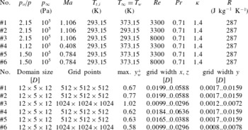
Details are given in table 1. For simulations with a total temperature difference between wall $T_{w}$ and inlet $T_{t,i}$ (#1, #4, #5 and #6), heat transfer is of interest. Therefore, the resolution close to the wall is even finer: $\max y^{+}\leqslant 0.67$ . In the other two cases ( $T_{w}-T_{t,i}=0$ ; simulations #2 and #3), much smaller temperature gradients occur at the wall and a slightly larger maximal $y^{+}$ -value is set due to a modification of the grid stretching. $y^{+}$ -values of around one are, according to the literature, sufficient for sub- and supersonic boundary layer flows like pipes or channels, e.g. Eggels et al. (Reference Eggels, Unger, Weiss, Westerweel, Adrian, Friedrich and Nieuwstadt1994). The special characteristic of the impinging jet is mainly the deflection zone. Since the velocity is zero in the stagnation point and low in its vicinity, the resulting $y^{+}$ -values are even lower ( $y^{+}\ll 1$ ) in the deflection zone. The above mentioned maximal values can be found in the wall jet at similar conditions to those of the cases studied in literature.

For the wall-parallel directions, a slight symmetrical grid stretching is applied, which refines the jet shear layer. The refinements use hyperbolic tangent respectively hyperbolic sin functions resulting in a change of mesh spacing lower than $1\,\%$ for all cases and directions. Table 1 shows the physical and geometrical parameters of the simulations.

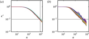
The use of DNS does not involve any kind of turbulence model and leads to huge grid sizes of more than one billion points for $Re=8000$ . The storage of one time step with the necessary five variables requires about 41 GB of storage. For this reason, statistics are computed on-the-fly in order to avoid the storage of thousands of samples. Figure 1 exemplary shows the convergence of the main variables $p,u,v,w,s$ (a) and the Reynolds stress transport terms $TD_{ij}$ , $VD_{ij}$ , $PS_{ij}$ , $DS_{ij}$ (b, see § 7). The latter include averages of fluctuations. Therefore, the averaging procedure of these terms starts after simple averages of the main variables were already converged. As converged we consider a reduction of the residuum of two orders of magnitude. This is achieved, depending on the case, after about three perfusion times and $7.5\times 10^{4}$ time steps. A loss of three orders of magnitude would require approximately a half million time steps for each averaging step and would exceed the computational resources that can be provided nowadays.

Figure 1.

Convergence of averaged values: $\unicode[STIX]{x1D716}^{r}$ is the root mean square of the residuum within the domain, normalised with the respective value of the first time step of the averaging. (a) Simple averages ( $p,u,v,w,s$ ), (b) averages of terms including fluctuations (Reynolds stress transport terms $TD_{ij}$ , $VD_{ij}$ , $PS_{ij}$ , $DS_{ij}$ , see § 7). The vertical grey line indicates the start of averaging step two.

Table 1.

Geometrical and physical parameters of the simulation. $p_{o}$ , $p_{\infty }$ , $T_{t,i}$ , $T_{\infty }$ , $T_{w}$ , $\mathit{Ma}$ , $Re$ , $Pr$ , $\unicode[STIX]{x1D705}$ , $R$ and $y_{w}^{+}$ denote total and ambient pressure, total, ambient and wall temperature, Mach, Reynolds and Prandtl number, ratio of specific heats, the specific gas constant and the dimensionless wall distance at the wall.

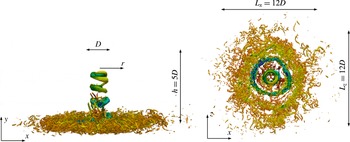
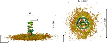
For post-processing purposes, a cylindrical coordinate system is used. Both coordinate systems as well as the domain sizes are shown in figure 2. The choice of the mesh width $\unicode[STIX]{x1D6E5}=(\unicode[STIX]{x1D6E5}_{x}\unicode[STIX]{x1D6E5}_{y}\unicode[STIX]{x1D6E5}_{z})^{1/3}$ was based on the Kolmogorov length scale $l_{\unicode[STIX]{x1D702}}=(\unicode[STIX]{x1D708}^{3}/\unicode[STIX]{x1D716})^{1/4}$ . The shear layer of the free and wall jet are resolved with $\unicode[STIX]{x1D6E5}\leqslant 1.9l_{\unicode[STIX]{x1D702}}$ , respectively $\unicode[STIX]{x1D6E5}\leqslant 1.4l_{\unicode[STIX]{x1D702}}$ . The only values of $\unicode[STIX]{x1D6E5}$ exceeding $2l_{\unicode[STIX]{x1D702}}$ up to $4l_{\unicode[STIX]{x1D702}}$ can be found in the viscous sublayer at the stagnation point close to the wall for supersonic cases. However, since the flow in the viscous sublayer is not turbulent, the resolution in terms of the Kolmogorov length scale is not of relevance. Dairay et al. (Reference Dairay, Fortuné, Lamballais and Brizzi2015) used a similar resolution for their DNS. Energy spectra of the simulations described in this article are shown in Wilke (Reference Wilke2017) and prove that the chosen resolution is appropriate.

In order to advance in time, a fourth-order five stage explicit Runge–Kutta scheme is applied. This scheme combines accuracy with efficiency in terms of computational costs. The spatial discretisation uses compact fifth-order upwind finite differences for the convective terms and sixth-order compact central schemes for the diffusive terms. The upwind scheme introduces dissipation for high wavenumbers and stabilises the simulation in case some parts of the domain are (temporally) slightly under-resolved. For a higher under-resolution, which is not the case of the presented simulations, an additional filter would be necessary. The central scheme has no dissipation. Both discretisation methods provide a low dispersion error and can be efficiently parallelised on modern high performance computers. The load is partitioned between thousands of processes, e.g. 16 384 for the case with $Re=8000$ . Each process solves the governing equations for a subdomain (block), see Eidson & Erlebacher (Reference Eidson and Erlebacher1995). Since information from adjacent blocks are needed for the calculation of compact derivatives, the decomposed domain is rearranged so that each process receives grid lines that span the entire domain in the particular direction. The total number of grid points per process remains constant and is typically between $32^{3}$ and $64^{3}$ . The inter-process communication is managed via MPI libraries.

Figure 2.

Three-dimensional contour plot of the impinging jet (#6) at $QD^{2}/v_{\infty }^{2}=5$ , coloured with pressure ( $0.8\leqslant p/p_{\infty }\leqslant 1.1$ , blue to red).

Figure 3.

Mean profiles of radial velocity (a,b) and temperature (c,d) at $y/D=0.05$ : 

(blue),  $T_{w}=T_{\infty }=373.15$ K and $T_{t,i}=293.15$ K. (a,c) Influence of the Mach number:

, #4 ( $\mathit{Ma}=0.4$ ); 

, #5 ( $\mathit{Ma}=0.8$ ); 

, #1 ( $\mathit{Ma}=1.1$ ). (b,d) Influence of the Reynolds number:

, #5 ( $Re=3300$ ); 

, #6 ( $Re=8000$ ).

3 Deflection zone and wall jet

In § 4, RAs are tested for their applicability to impingement jets. First relations of this kind were developed for canonical compressible wall-bounded turbulent flows like pipes or channels. However, a more recent approach also takes into account an existing wall heat flux and pressure gradient in the streamwise direction. In this section, we want to highlight some particularities of the wall-bounded turbulent flow of impinging jets.

According to the radial velocity, we divide the wall jet into four zones. The accelerating zone ( $0\leqslant r/D\lesssim 0.8$ ), the zone of maximal radial velocity ( $r/D\approx 0.8$ ), the decelerating zone ( $r/D\gtrsim 0.8$ ) and a zone where the influence of the impingement is not dominant any more ( $r/D\gtrsim 2.5$ ). According to the parameters $\mathit{Ma},Re,T_{w}$ the position of the maximum radial velocity changes slightly. For the flow description, the radial positions $r/D=0.3$ , $0.8$ , $1.4$ and $3.5$ are chosen.

Figure 4.

Dimensionless pressure (a,b) and r.m.s. of pressure fluctuations (c,d) at the impinging plate. (a,c) Influence of the Mach number:

, #4 ( $\mathit{Ma}=0.4$ ); 

, #5 ( $\mathit{Ma}=0.8$ ); 

, #1 ( $\mathit{Ma}=1.1$ ). (b,d) Influence of the Reynolds number:

, #5 ( $Re=3300$ ); 

, #6 ( $Re=8000$ ).

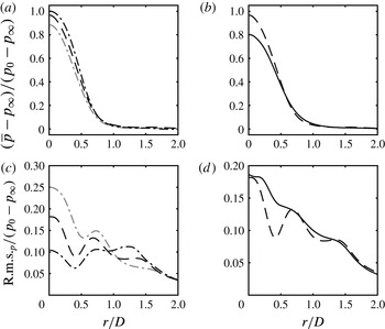
Figure 3(a,b) shows the mean radial velocity $u_{r}$ at the wall distance of $y/D=0.05$ . Starting from the stagnation point it strongly increases due to the stagnation pressure and reaches a maximum value that is lower than the inlet velocity $v_{\infty }$ . On the left, the influence of the Mach number $\mathit{Ma}$ is shown. The radial velocity is almost unaffected by $\mathit{Ma}$ , but slightly decreases with increasing $\mathit{Ma}$ . The influence of the Reynolds number (right) is stronger. $u_{r}$ decreases with increasing $Re$ and the position of the maximum moves to greater $r/D$ .

Figure 5.

Velocity (a–c) and temperature (d–f) boundary layer at $r/D=1.4$ . (a,d) Influence of the Mach number:

, #4 ( $\mathit{Ma}=0.4$ ); 

, #5 ( $\mathit{Ma}=0.8$ ); 

, #1 ( $\mathit{Ma}=1.1$ ). (b,e) Influence of the Reynolds number:

, #5 ( $Re=3300$ ); 

, #6 ( $Re=8000$ ). (c,f) Influence of a heated environment:

, #2 (not heated); 

, #1 (heated).

Figure 3(c,d) shows the mean temperature at the same position. The temperature profile is influenced by three effects: (i) the mixing of the wall jet with the hot environment. This causes the main trend of increasing temperature with increasing $r/D$ . (ii) Heat transfer at the isothermal wall and (iii) compressibility effects. (a,c) Shows the influence of the Mach number. At low $Ma$ (#4; $Ma\approx 0.4$ ), the average temperature reaches the value of the total inlet temperature $T_{t,i}$ . At higher Mach number (sub- and supersonic jets), both temperatures in the stagnation point are higher then $T_{t,i}$ . This is an indication that the flow around the stagnation point has lower fluctuations (is less unsteady) when the Mach number is low. A more unsteady flow around the stagnation point entrains surrounding fluid. Since the surrounding fluid is of higher temperature in the considered simulations, the temperature in the deflection zone increases.

The effect of compressibility can be seen in the areas with high (radial) velocity. A high velocity leads to a decreasing temperature, e.g. at $r/D\approx 0.8$ , the supersonic case (#1) features a global minimum at the point where the axial velocity is maximal (Figure 3 a,b). The same effect is present for the highly subsonic jet (#5), but weaker distinct. The position of decreased temperature variates in accordance with the position of high axial velocity.

To further understand the unsteadiness of the flow around the stagnation point, we look at the wall pressure and its fluctuations. Figure 4(a), it can be seen that the pressure recovery decreases with increasing Mach number. At low Mach number (#4, $\mathit{Ma}=0.4$ ) a value of 0.97 is observed whereas the pressure recovery is only 0.9 at $\mathit{Ma}=1.1$ (#1). We can understand the relation between pressure recovery and pressure fluctuation with a simple thought experiment. We approximate the high pressure around the stagnation point as a half-unit circle with the flat side to the bottom and add a normally distributed random movement of the centre. In case of a very small movement, e.g. with a variance of 0.1, the shape of the function is still approximately a half-unit circle and the maximum value is still close to one (0.995). This case represents simulation #4. If we increase the variance of the random displacement (e.g. #5) to 0.3, the shape changes and the maximum value decreases to 0.951. Consequently, the two curves have to cross each other at some point. This crossing can be observed between simulations #4 and #5 as well as (#5, #6) on the figure 4(b). However no crossing between (#1, #4) implies that the lower pressure recovery in the supersonic case is mainly caused by losses due to the shocks present in the free jet region as well as standoff shocks.

The corresponding raised root mean square (r.m.s.) values indicate an increased movement of the stagnation point. The plots on the right show that also an increasing Reynolds number leads to larger fluctuations of the stagnation point and consequently to a lower pressure recovery.

The boundary layer is resolved in all cases with a maximum $y^{+}$ value of one in the first grid point next to the wall, see table 1. Figure 5 shows the velocity and temperature boundary layer of the impinging jets. The dimensionless wall distance $u^{+}$ , dimensionless temperature $T^{+}$ and friction temperature $T_{\unicode[STIX]{x1D70F}}$ are defined as

(3.1a-c ) $$\begin{eqnarray}u^{+}=\frac{\sqrt{u^{2}+w^{2}}}{u_{\unicode[STIX]{x1D70F}}},\quad T^{+}=\frac{T_{w}-T}{T_{\unicode[STIX]{x1D70F}}},\quad T_{\unicode[STIX]{x1D70F}}=\frac{q_{w}}{\unicode[STIX]{x1D70C}c_{p}u_{\unicode[STIX]{x1D70F}}},\end{eqnarray}$$

where $q_{w}$ is the wall heat flux. The $u^{+}$ -profile of the wall jet is for all computations and $r/D$ lower than the solution of the channel flow (figure 5). The maximum is caused by the fact that the wall jet has a finite thickness. The above fluid is almost at rest, neglecting a slight recirculation. If we move, starting from the wall, in the positive $y$ or $y^{+}$ direction, the wall-parallel velocity increases from zero until we reach approximately the middle of the wall jet. With further increasing wall distance, the velocity decreases due to the mixing between wall jet and the surrounding fluid in rest (upper shear layer). Neglecting recirculation, the velocity reaches again zero at the end of the wall jet. Furthermore, no logarithmic region of the boundary layer is observed. The investigated Reynolds numbers up to 8000 are too low to allow the formation of such a layer under the condition of a limited wall-normal extent of the wall-bounded flow. Looking at figure 5(d–f), we see that the computed $T^{+}$ -profiles are higher in relation to the theoretical reference $T^{+}=Pr\;y^{+}$ than the velocity profile in relation to $u^{+}=y^{+}$ . The choice of the wall temperature has a strong influence on both profiles. A heated wall leads to higher $T^{+}$ and lower $u^{+}$ values. The influence of the Mach number is in general smaller and depends on the radial position. More profiles for validation purposes are given in Wilke (Reference Wilke2017).

4 Reynolds analogies and correlations

Since impinging jets are used among other things for cooling of hot surfaces, an accurate computation of heat transfer is needed. Furthermore, relations between quantities affiliated to heat transfer and quantities affiliated to momentum transfer are of great interest.

4.1 Mean field

Heat transfer at the impinging plate is quantified by the Nusselt number:

(4.1) $$\begin{eqnarray}\mathit{Nu}=\frac{D}{\unicode[STIX]{x0394}T}\cdot \left.\frac{\unicode[STIX]{x2202}T}{\unicode[STIX]{x2202}y}\right|_{w}=q_{w}\frac{DPr}{\unicode[STIX]{x0394}Tc_{p}\unicode[STIX]{x1D702}}.\end{eqnarray}$$

Here $D$ is the inlet diameter, $\unicode[STIX]{x0394}T$ is the difference between total inlet temperature $T_{t,i}$ and wall temperature $T_{w}$ , $Pr,c_{p},\unicode[STIX]{x1D702}$ and $q_{w}$ are the Prandtl number, the ratio of specific heats, the dynamic viscosity and the heat flux in the wall-normal direction at the wall. Reynolds discovered that the similarity of the momentum and energy equation for incompressible laminar boundary layers can be used to approximate heat transfer with the use of fluid friction, see Kakag & Yenner (Reference Kakag and Yenner1995):

(4.2) $$\begin{eqnarray}\mathit{St}=\frac{\mathit{Nu}}{RePr}\approx \frac{C_{f}}{2}=\frac{\unicode[STIX]{x1D70F}_{w}}{\unicode[STIX]{x1D70C}v_{\infty }^{2}}.\end{eqnarray}$$

This is the well-known RA. The assumption made is a Prandtl number equal to one. $C_{f}$ and $\unicode[STIX]{x1D70F}_{w}$ are the skin friction factor and the wall shear stress. This equation was modified by Chilton & Colburn (Reference Chilton and Colburn1934), based on experimental data:

(4.3) $$\begin{eqnarray}\mathit{St}Pr^{2/3}=\frac{\mathit{Nu}}{RePr^{1/3}}\approx \frac{C_{f}}{2}\end{eqnarray}$$

and considers Prandtl numbers different from one. Equation (4.3) is referred to as the Chilton Colburn analogy (CCA). Figure 6 shows the skin friction coefficients of the conducted simulations. (a) Indicates that $C_{f}$ is almost independent of the Mach number in the range $0.4\leqslant \mathit{Ma}\leqslant 1.1$ . An increasing Reynolds number leads to a decreasing skin friction factor for small radii of $r/D\lesssim 2$ (b). Comparing a jet with equal total inlet temperature $T_{t,i}$ , ambient $T_{\infty }$ and wall temperature $T_{w}$ to another one with $T_{\infty }=T_{w}>T_{t,i}$ , it can be seen that the skin friction factor increases due to the heated environment. The total inlet temperature has been kept constant.

Figure 6.

Mean Skin friction factor $\overline{C_{f}}$ . (a) Influence of the Mach number:

, #4 ( $\mathit{Ma}=0.4$ ); 

, #5 ( $\mathit{Ma}=0.8$ ); 

, #1 ( $\mathit{Ma}=1.1$ ). (b) Influence of the Reynolds number:

, #5 ( $Re=3300$ ); 

, #6 ( $Re=8000$ ). (c) Influence of a heated environment:

, #2 (not heated); 

, #1 (heated).

In figure 7, Nusselt number profiles of the simulations with $T_{\infty }=T_{w}>T_{t,i}$ are compared (otherwise $\unicode[STIX]{x0394}T=0$ ). The influence of the Mach number (a) is strongest in the vicinity of the stagnation point. The simulation with low compressibility ( $\mathit{Ma}\approx$ 0.4) has the global maximum at around $r/D=0.3$ and not at the axis. Here $\mathit{Nu}$ increases with increasing $\mathit{Ma}$ at the stagnation point. As we have seen in the previous section, a high Mach number leads to strong fluctuations within the deflection zone. Furthermore, the temperature difference between cooling fluid and hot wall is strongest in the case with the lowest Mach number. This means that the higher heat transfer at the stagnation point for higher Mach numbers is not caused by the mean field but rather by unsteady effects that lead to a high turbulent heat flux. All simulations feature a secondary local maximum respectively shoulder or saturation zone around $r/D=1.5$ . Nusselt number correlations of the shape $\mathit{Nu}\sim Re^{n}$ are in wide use. Also the Prandtl number and geometrical parameters can be included. According to Lee & Lee (Reference Lee and Lee1999), the exponents for plate distances $h/D$ of 4 and 6 are $n=0.53$ and $n=0.58$ , respectively. For the presently investigated simulations of $h/D=5$ , the exponent $n=0.555$ was chosen. The influence of the Reynolds number is illustrated in the figure 7(b,c). As expected, heat transfer increases with $Re$ . The scaling fits away from the stagnation point $r/D\gtrsim 1$ . According to this simple correlation, heat transfer within the stagnation point area of the higher Reynolds number (8000) is weaker than in case of $Re=3300$ . The reason for this observation lies within a greater entrainment of hot fluid in case of $Re=8000$ . This can be confirmed by a higher mean temperature in the deflection zone (figure 3 d).

Figure 7.

Mean Nusselt number $\overline{\mathit{Nu}}$ . (a) Influence of the Mach number:

, #4 ( $\mathit{Ma}=0.4$ ); 

, #5 ( $\mathit{Ma}=0.8$ ); 

, #1 ( $\mathit{Ma}=1.1$ ). (b,c) Influence of the Reynolds number:

, #5 ( $Re=3300$ ); 

, #6 ( $Re=8000$ ).

The validation of the Nusselt number with experimental data is difficult, since measurements found in literature vary significantly. The experimental set-up and in particular the shape of the nozzle as well as the measurement position and method of averaging have a strong influence on the measured heat transfer (Janetzke Reference Janetzke2010). For this reason reported Nusselt numbers differ by a factor of up to 2.4 and can only give an approximate estimation of impingement heat transfer. Figure 8 shows that our DNS data lay within the corridor described by heat transfer measurements. Furthermore, it is observed that the common neglect of Mach number effects leads to a variation of the stagnation point Nusselt number $\mathit{Nu}_{0}$ of $26\,\%$ , comparing simulations #4 ( $\mathit{Ma}=0.41$ ) and #1 ( $\mathit{Ma}=1.11$ ).

Figure 8.

Stagnation point Nusselt number as function of the Reynolds number. Adapted from Janetzke (Reference Janetzke2010): 

, single impinging jet; 

, impinging jet array. Own simulations: square, #4 ( $\mathit{Ma}=0.41$ ); point, #5, #6 ( $\mathit{Ma}=0.78$ ); triangle, #1 ( $\mathit{Ma}=1.11$ ).

Figure 9.

Heat transfer at the impinging plate (Nusselt number): (a) simulation #5 ( $Re=3300$ ); (b) #6 ( $Re=8000$ ); 

, DNS data; 

, RA; 

, CCA.

The RA and the CCA are shown in figure 9. As they are developed for wall-bounded flows, the analogies are not suitable for the stagnation point region. In this region, the relative error is between approximately $-80\,\%$ and $-40\,\%$ . At the position where $C_{f}$ reaches its maximum, both analogies over-predict the heat transfer: ${\approx}\,+30\,\%$ (RA) respectively ${\approx}\,+65\,\%$ (CCA). Farther away from the axis $r/D\gtrsim 2$ , the analogies fit much better. The best agreement is found in case of the higher Reynolds number using the CCA. Here the error is between $-9\,\%$ and $-4\,\%$ . Taking the flow properties of the impinging jet, described in § 3, into account, we observe that the deceleration of the wall jet is not problematic for the analogies. The radial velocity has its maximum at $r/D\approx 0.8$ . At $r/D\gtrsim 1$ , the flow is strongly decelerating, but both analogies estimate heat transfer with much better accuracy than at $r/D\lesssim 1$ . The area of poor heat transfer estimation coincides with the area featuring a high pressure gradient.

Other relations involving mean temperature and mean velocity were developed by Busemann (Reference Busemann1931) and Crocco (Reference Crocco1932), Walz (Reference Walz1962) and Zhang et al. (Reference Zhang, Bi, Hussain and She2014). In Zhang et al. (Reference Zhang, Bi, Hussain and She2014), the derivation is explained in detail. All relations have the common form:

(4.4) $$\begin{eqnarray}\frac{\overline{T}}{\overline{T}_{\unicode[STIX]{x1D6FF}}}=\frac{\overline{T}_{w}}{\overline{T}_{\unicode[STIX]{x1D6FF}}}+\frac{T_{r}-\overline{T}_{w}}{\overline{T}_{\unicode[STIX]{x1D6FF}}}\;\frac{\overline{u_{r}}}{\overline{u_{r}}_{\unicode[STIX]{x1D6FF}}}+\frac{\overline{T}_{\unicode[STIX]{x1D6FF}}-T_{r}}{\overline{T}_{\unicode[STIX]{x1D6FF}}}\left(\frac{\overline{u_{r}}}{\overline{u_{r}}_{\unicode[STIX]{x1D6FF}}}\right)^{2},\end{eqnarray}$$

with

(4.5) $$\begin{eqnarray}T_{r}=\overline{T}_{\unicode[STIX]{x1D6FF}}+r\frac{\overline{u_{r}}_{\unicode[STIX]{x1D6FF}}^{2}}{2c_{p}}.\end{eqnarray}$$

The subscript $\unicode[STIX]{x1D6FF}$ denotes the boundary layer edge ( $\unicode[STIX]{x1D6FF}=\unicode[STIX]{x1D6FF}_{99}$ ). The recovery factor $r$ changes according to the authors. For $r=1$ , the Crocco–Busemann relation (CBR) is derived. In the Walz’s equation or modified CBR, $r=0.88$ . The generalised Reynolds analogy (GRA) proposed by Zhang et al. (Reference Zhang, Bi, Hussain and She2014) uses the general recovery factor according to (4.6):

(4.6) $$\begin{eqnarray}r=\left(\overline{T}_{w}-\overline{T}_{\unicode[STIX]{x1D6FF}}\right)\frac{2c_{p}}{\overline{u_{r}}_{\unicode[STIX]{x1D6FF}}^{2}}-\frac{2Pr}{\overline{u_{r}}_{\unicode[STIX]{x1D6FF}}}\;\frac{\overline{q}_{w}}{\overline{\unicode[STIX]{x1D70F}_{w}}}.\end{eqnarray}$$

Those three relations were tested for the impinging jet. The difference between the Crocco–Busemann and Walz’s equation was found to be negligible for the present simulations. For the reason of lucidity, the approximation according to Walz is not shown.

In figure 10, the boundary layer thickness of radial (wall-parallel) velocity $\overline{u_{r}}_{\unicode[STIX]{x1D6FF}}$ and temperature $\overline{T}_{\unicode[STIX]{x1D6FF}}$ are shown. Both boundary layers increase with increasing radial distance in all cases. Additionally to the thinner boundary layer in the case of the higher Reynolds number #6 ( $Re=8000$ ), compared with #5 ( $Re=3300$ ), another difference occurs. At $Re=3300$ , the velocity boundary layer features a local decrease at $1.9\leqslant r/D\leqslant 2$ . In this area, the average radial velocity is strongly influenced by the periodical movement of primary and secondary vortex rings. The drop in $\overline{u_{r}}_{\unicode[STIX]{x1D6FF}}$ is caused by the separation of the vortex pair at this location. Figure 17 shows these vortices. At higher Reynolds number, the vortex rings occur with the same frequency, but due to the higher level of turbulence, the radial position of the separation as well as the shape of the vortices vary more strongly than at $Re=3300$ . Consequently, no exact repetitive location of separation is present and no drop in the velocity boundary layer occurs.

Figure 11 shows the DNS data compared with the approximations of Crocco–Busemann and the GRA. The mean temperature and mean wall-parallel (radial) velocity are normalised by the values at the edge of the boundary layer (subscript $\unicode[STIX]{x1D6FF}=\unicode[STIX]{x1D6FF}_{99}$ ) as in Zhang et al. (Reference Zhang, Bi, Hussain and She2014). For both Reynolds numbers the GRA fits better than the CBR for radial positions close to the stagnation point ( $r/D=0.3$ and $r/D=0.8$ ). Farther away ( $r/D=1.4$ and $r/D=3.5$ ), the opposite can be observed. This is a consequence of different curvatures of the DNS profiles and the fact that the scaled mean temperature is always predicted higher according to the GRA. Further can be ascertained that the GRA gives a precise prediction of the temperature field for $Re=8000$ and $r/D=0.8$ . At this radial position, the radial velocity has its maximum. Given that no de- and acceleration is present, the conditions are most similar to canonical compressible wall-bounded turbulent flows for which the relation was developed. In CCWTFs the flow can be approximated as quasi-one-dimensional. Examples for such flows are pipes and channels.

Figure 10.

Boundary layer thickness (

): (a,b) radial velocity $\overline{u_{r}}_{\unicode[STIX]{x1D6FF}}$ ; (c,d) temperature $\overline{T}_{\unicode[STIX]{x1D6FF}}$ ; (a,c) simulation #5 ( $Re=8000$ ); (b,d) simulation #6 ( $Re=8000$ ). Contour lines of $\overline{u_{r}}$ respectively $\overline{T}$ are shown in the background.

Figure 11.

Relation between mean temperature and mean velocity in the wall jet: (a) simulation #5 ( $Re=3300$ ); (b) simulation #6 ( $Re=8000$ ). Colours:

(sky blue),  $r/D=0.3$ ; 

(blue), $r/D=0.8$ ; 

(red),  $r/D=1.4$ ; 

,  $r/D=3.5$ . Patterns:

, DNS data; 

, CBR;

, GRA.

4.2 Fluctuations

In addition to the relation between mean temperature and velocity, Zhang et al. (Reference Zhang, Bi, Hussain and She2014) also derived a general analogy for fluctuations:

(4.7) $$\begin{eqnarray}T^{\prime }-\frac{1}{\overline{Pr_{t}}}\frac{\unicode[STIX]{x2202}\overline{T}}{\unicode[STIX]{x2202}\overline{u}}u^{\prime }+\unicode[STIX]{x1D719}^{\prime }-\frac{\overline{\left(\unicode[STIX]{x1D70C}v\right)^{\prime }\unicode[STIX]{x1D719}^{\prime }}}{\overline{\left(\unicode[STIX]{x1D70C}v\right)^{\prime }u^{\prime }}}u^{\prime }=0,\end{eqnarray}$$

where $\unicode[STIX]{x1D719}^{\prime }$ is a residual temperature that needs to be modelled. The proposed model chosen by Zhang et al. (Reference Zhang, Bi, Hussain and She2014) for ‘convenience’ is

(4.8) $$\begin{eqnarray}\unicode[STIX]{x1D719}^{\prime }=\frac{\overline{\left(\unicode[STIX]{x1D70C}v\right)^{\prime }\unicode[STIX]{x1D719}^{\prime }}}{\overline{\left(\unicode[STIX]{x1D70C}v\right)^{\prime }u^{\prime }}}u^{\prime },\end{eqnarray}$$

so that (4.7) is reduced to

(4.9) $$\begin{eqnarray}T^{\prime }=\frac{1}{\overline{Pr_{t}}}\frac{\unicode[STIX]{x2202}\overline{T}}{\unicode[STIX]{x2202}\overline{u}}u^{\prime }.\end{eqnarray}$$

Zhang et al. (Reference Zhang, Bi, Hussain and She2014) further describe that (4.9) is not valid, but the r.m.s. of $T^{\prime }$ and $u^{\prime }$ can be approximated in a similar way:

(4.10a,b ) $$\begin{eqnarray}\sqrt{\overline{T^{\prime 2}}}\approx \left|\frac{1}{\overline{Pr_{t}}}\frac{\unicode[STIX]{x2202}\overline{T}}{\unicode[STIX]{x2202}\overline{u}}\right|\sqrt{\overline{u^{\prime 2}}}\quad \text{or}\quad \sqrt{\overline{T^{\prime 2}}}\approx \pm \frac{\overline{\left(\unicode[STIX]{x1D70C}v\right)^{\prime }T^{\prime }}}{\overline{\left(\unicode[STIX]{x1D70C}v\right)^{\prime }u^{\prime }}}\sqrt{\overline{u^{\prime 2}}}.\end{eqnarray}$$

The plus sign applies to the flow region where the wall-normal gradients of the mean temperature and velocity have the same sign. The minus sign applies to the opposite situation. This approximation fails in case of the impinging jet. In the boundary layer the term $\overline{\left(\unicode[STIX]{x1D70C}v\right)^{\prime }u^{\prime }}$ changes its sign. The approximation delivers huge values of $\sqrt{\overline{T^{\prime 2}}}$ in the vicinity of the zero crossing. A further approximation is suggested by Zhang et al. (Reference Zhang, Bi, Hussain and She2014) that reduces the connection between temperature and velocity fluctuations to $R_{v^{\prime }u^{\prime }}\approx R_{v^{\prime }T^{\prime }}$ . 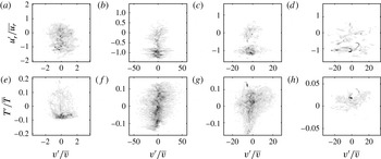Where $R$ is the correlation coefficient. Also this approximation is invalid for the impinging jet. Figure 12 exemplary shows joint probability distributions of simulation #6 ( $Re=8000,\mathit{Ma}\approx 0.8$ ) in the boundary layer at $13\leqslant y^{+}\leqslant 17$ . 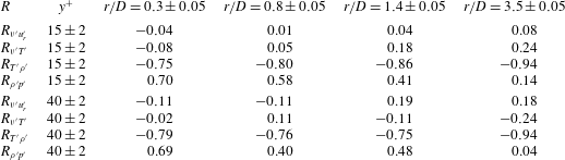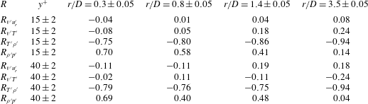The best rendering was achieved with a classification of the data into 250 segments for each variable covering 95 % of the velocity and 99 % of all other fluctuations. The database consists of 550 equally spaced snapshots (symmetry planes) out of 175 000 that have been computed after the flow reached its quasi-stationary state. The corresponding correlation coefficients are given in table 2 for the same $y^{+}$ value and additional for $38\leqslant y^{+}\leqslant 42$ . It can be seen that neither the radial velocity nor the temperature is correlated to the axial velocity. Despite both coefficients are close to zero, it cannot be said that they are approximatively equal.

Figure 12.

Joint probability distributions of radial velocity (a–d) and temperature (e–h) fluctuation against the axial velocity fluctuation at $13\leqslant y^{+}\leqslant 17$ for different radial positions (a–h $r/D=0.3$ , $0.8$ , $1.4$ and $3.5$ ), simulation #6 ( $Re=8000$ ).

4.3 Additional correlations

The derivation of RAs is closely related to the development of models for compressible turbulence. For instance, a similar equation to 4.10 was derived by Rubesin (Reference Rubesin1990). He assumed that thermodynamic fluctuations behave in a polytropic manner:

(4.11) $$\begin{eqnarray}\frac{p^{\prime }}{\overline{p}}=n\frac{\unicode[STIX]{x1D70C}^{\prime }}{\overline{\unicode[STIX]{x1D70C}}}=\frac{n}{n-1}\;\frac{\unicode[STIX]{x1D70C}T^{\prime \prime }}{\overline{\unicode[STIX]{x1D70C}}\widetilde{T}}.\end{eqnarray}$$

After assuming that $T^{\prime }/\overline{T}\approx T^{\prime \prime }/\widetilde{T}$ and linearisation according to Lechner et al. (Reference Lechner, Sesterhenn and Friedrich2001), the relation

(4.12) $$\begin{eqnarray}\left(n-1\right)\frac{\unicode[STIX]{x1D70C}^{\prime }}{\overline{\unicode[STIX]{x1D70C}}}\approx \frac{\unicode[STIX]{x1D70C}T^{\prime }}{\overline{\unicode[STIX]{x1D70C}}\;\overline{T}}\end{eqnarray}$$

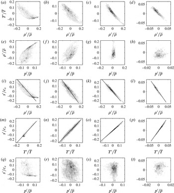
is derived. As suggested, with $n=0$ it follows that the correlation coefficient $R_{\unicode[STIX]{x1D70C},T}$ is minus one, $R_{\unicode[STIX]{x1D70C},p}\approx 0$ and that pressure fluctuations are unimportant compared to density fluctuations. The correlation coefficients are given in table 2, the joint probability distributions are shown in figure 14. Here $R_{\unicode[STIX]{x1D70C},T}$ is strongly negative for all observation points. Far away from the stagnation point ( $r/D=3.5$ ), the coefficient reaches a value of $-0.94$ and justifies the approximations. The correlation between density and pressure is not zero, as proposed. On the contrary, the coefficient is strongly positive ( ${\approx}0.7$ ) close to the axis, but decreases with increasing $r/D$ . Far away from the stagnation point, the approximation $R_{\unicode[STIX]{x1D70C},p}\approx 0$ is valid. Similarly, pressure fluctuations are not unimportant compared to density fluctuation in the entire region where the flow is influenced by impingement. Farther downstream, $\text{r.m.s.}_{\unicode[STIX]{x1D70C}}/\overline{\unicode[STIX]{x1D70C}}$ is around three times as large as $\text{r.m.s.}_{p}/\overline{p}$ for $y^{+}\gtrsim 5$ , as it can be seen in figure 13.

Figure 13.

The r.m.s. values of pressure and density for subsonic impinging jets for different radial positions (a–d $r/D=0.3$ , $0.8$ , $1.4$ and $3.5$ ): 

,  $\text{r.m.s.}_{p}/\overline{p}$ (#5, $Re=3300$ ); 

,  $\text{r.m.s.}_{p}/\overline{p}$ (#6, $Re=8000$ ); 

(red),  $\text{r.m.s.}_{\unicode[STIX]{x1D70C}}/\overline{\unicode[STIX]{x1D70C}}$ (#5, $Re=3300$ ); 

(red),  $\text{r.m.s.}_{\unicode[STIX]{x1D70C}}/\overline{\unicode[STIX]{x1D70C}}$ (#6, $Re=8000$ ).

Table 2.

Correlation coefficients for simulation #6.

Lechner et al. (Reference Lechner, Sesterhenn and Friedrich2001) assumed a linear relation between thermodynamic fluctuations. Following the entropy definition $s=c_{v}\ln \left(p/\unicode[STIX]{x1D70C}^{\unicode[STIX]{x1D705}}\right)$ , the linearised gas law and the neglect of pressure fluctuations with respect to density fluctuations, the approximation reads

(4.13) $$\begin{eqnarray}\frac{s^{\prime }}{c_{v}}\approx -\unicode[STIX]{x1D705}\frac{\unicode[STIX]{x1D70C}^{\prime }}{\overline{\unicode[STIX]{x1D70C}}}\approx \unicode[STIX]{x1D705}\frac{T^{\prime }}{\overline{T}}.\end{eqnarray}$$

Figure 14 shows the joint probability distributions of ( $s^{\prime },\unicode[STIX]{x1D70C}^{\prime }$ ), ( $s^{\prime },T^{\prime }$ ) and ( $s^{\prime },p^{\prime }$ ). Approximation (4.13) is included in the plots (black solid line) and is found to be reasonable for all radial positions.

Figure 14.

Joint probability distributions at $13\leqslant y^{+}\leqslant 17$ for different radial positions (a–t) $r/D=0.3$ , $0.8$ , $1.4$ and $3.5$ , simulation #6 ( $Re=8000$ ). Approximation (4.13) is included in row 3 and 4 (black solid line).

5 Turbulent heat flux

In § 4.1, figure 7, Nusselt number profiles of simulations #5 ( $Re=3300$ ) and #6 ( $Re=8000$ ) are shown. In both cases, $\mathit{Nu}$ decreases with increasing radial distance. Superimposed to this main trend, a shoulder exists at $1\lesssim r/D\lesssim 2$ , where the slope is reduced. Depending on the parameters of the impinging jet, the slope can also be positive in this area and form a secondary maximum. In Wilke & Sesterhenn (Reference Wilke and Sesterhenn2015a ), this shoulder or secondary maximum was ascribed to the occurrence of secondary vortex rings that locally increase heat transfer. Using the turbulent heat flux, we can quantify this effect. Figure 15(a–c) shows the turbulent heat flux in the wall-normal direction $\overline{\unicode[STIX]{x1D70C}v^{\prime \prime }e^{\prime \prime }}$ . Close to the wall, $\overline{\unicode[STIX]{x1D70C}v^{\prime \prime }e^{\prime \prime }}$ is positive in the area of the $\mathit{Nu}$ shoulder ((a,d) $r/D=1.4$ ). This means that heat is transported in the positive $y$ -direction (away from the impinging plate). After reaching a maximum at $y^{+}\approx 15$ to 20, the heat flux decreases and turns negative. This is due to the fact that vortices present at the upper border of the wall jet entrain hot fluid. The radial distribution at $y^{+}=15$ (b,e) proves that the zone where the turbulent heat flux is strongly positive coincides with the $\mathit{Nu}$ shoulder and that $\overline{\unicode[STIX]{x1D70C}v^{\prime \prime }e^{\prime \prime }}$ is negative in the vicinity of this zone for the lower Reynolds number. Further can be determined that in this zone the influence of $\overline{\unicode[STIX]{x1D70C}v^{\prime \prime }e^{\prime \prime }}$ is weaker at the higher Reynolds number. This agrees with the fact that the $\mathit{Nu}$ profile is smoother and that the vortex rings are overlaid with small-scale turbulence, leading to less strong structures.

Figure 15.

Influence of Reynolds number on turbulent heat flux in the wall-normal direction $\overline{\unicode[STIX]{x1D70C}v^{\prime \prime }e^{\prime \prime }}$ (a–c) and the radial direction $\overline{\unicode[STIX]{x1D70C}u_{r}^{\prime \prime }e^{\prime \prime }}$ (d–f): (a,d) $r/D=1.4$ ; (b,e) $y^{+}=15$ ; (c,f) $y^{+}=40$ ; 

, #5 ( $Re=3300$ ); 

, #6 ( $Re=8000$ ). For plots at fixed $r/D$ , the horizontal locations $y^{+}=15$ and $y^{+}=40$ are shown (

, blue). For plots at fixed $y^{+}$ , the vertical position $r/D=1.4$ is shown (

, blue).

Figure 15(d–f) shows the turbulent heat transfer in the radial direction $\overline{\unicode[STIX]{x1D70C}u_{r}^{\prime \prime }e^{\prime \prime }}$ . It is of the same order of magnitude as the one in the wall-normal direction. Close to the wall, $\overline{\unicode[STIX]{x1D70C}v^{\prime \prime }e^{\prime \prime }}$ is positive at $r/D=1.4$ for the case of $Re=3300$ . For the higher Reynolds number, this area of downstream turbulent heat flux is almost not present. At larger wall distances, $\overline{\unicode[STIX]{x1D70C}v^{\prime \prime }e^{\prime \prime }}$ is negative for both cases due to the direction of rotation of the vortices in the shear layers.

6 Reynolds stresses

Modern high performance computers allow three-dimensional direct numerical simulations of impinging jets with relevant Reynolds numbers since recently. However, the computations are limited to academic cases for the foreseeable future. For the improvement of turbulence models, that are widely used for industrial applications, our DNS provide a database to compare with. An important term that rises among others in the RANS equations is the Reynolds stress tensor $\overline{\unicode[STIX]{x1D70C}u_{i}^{\prime \prime }u_{j}^{\prime \prime }}$ that we describe in this section. Since the mean circumferential velocity component is zero, the terms $\overline{\unicode[STIX]{x1D70C}u_{\unicode[STIX]{x1D703}}^{\prime \prime }v^{\prime \prime }}$ and $\overline{\unicode[STIX]{x1D70C}u_{\unicode[STIX]{x1D703}}^{\prime \prime }u_{r}^{\prime \prime }}$ are not of relevance and therefore not shown. Figure 16 shows the four main entries of the tensor. We analyse the flow close to the wall and at the radial distance, where the shoulder of the Nusselt number is present. The profiles are taken normal to the wall at $r/D=1.4$ (a,d,g,j) and parallel to the wall at $y^{+}=15$ (b,e,h,k) and $y^{+}=40$ (c,f,i,l).

Figure 16.

Influence of Reynolds number on the main Reynolds stress tensor components: (a–l) $\overline{\unicode[STIX]{x1D70C}u_{\unicode[STIX]{x1D703}}^{\prime \prime 2}}$ , $\overline{\unicode[STIX]{x1D70C}v^{\prime \prime 2}}$ , $\overline{\unicode[STIX]{x1D70C}u_{r}^{\prime \prime 2}}$ and $\overline{\unicode[STIX]{x1D70C}v^{\prime \prime }u_{r}^{\prime \prime }}$ ; (a,d,g,j) $r/D=1.4$ ; (b,e,h,k) $y^{+}=15$ ; (c,f,i,l) $y^{+}=40$ ; 

, #5; 

, #6. For plots at fixed $r/D$ , the horizontal locations $y^{+}=15$ and $y^{+}=40$ are shown (

, blue). For plots at fixed $y^{+}$ , the vertical position $r/D=1.4$ is shown (

, blue).

At $r/D=1.4$ , the $\unicode[STIX]{x1D703}\unicode[STIX]{x1D703}$ -component (a) increases until $y^{+}\approx 10$ and then stays almost constant within the boundary layer. The maximum stress occurs around a half-diameter from the jet axis. At low Reynolds number (3300), a second maximum is present at approximate $r/D=2{-}2.5$ . Another difference between the two simulations is that the stress component is higher in the case of the higher Reynolds number (8000). Additional to this area, another area of high stress is present farther away from the wall and the jet axis and will be discussed later.

The $yy$ -component is stronger in case of the low Reynolds number. The strength of this entry of the tensor increases with the distance to the wall, until it decreases again when approaching the upper end of the wall jet. Since the wall jet’s centre and upper end is at higher $y^{+}$ -values in case of the higher Reynolds number, the maximum of $\overline{\unicode[STIX]{x1D70C}v^{\prime \prime 2}}$ occurs also at a higher dimensionless wall distance. The highest stress occurs at a radial distance of around $1.5{-}1.8$ diameters.

The distribution of the $rr$ -component features two maxima in the wall-normal direction, whereby this characteristic is distinct stronger in case of the lower Reynolds number. The gap between the two maxima increases with the distance from the jet axis. This shape is directly caused by the primary and secondary vortices that move parallel to the wall and increase their diameter. In figure 17, the area of the highest $\overline{\unicode[STIX]{x1D70C}u_{r}^{\prime \prime 2}}$ -value is indicated by two dash-dotted lines. Those lines coincide with the path of the primary vortex rings that have their origin in the shear layer of the free jet and the counter-rotating secondary vortices that emerge due to wall friction. The maximal fluctuations occur at $r/D\approx 1$ , where the two vortices have the highest radial velocity.

Figure 17.

Instantaneous flow field of simulation #6: $QD^{2}/v_{\infty }^{2}$ in the range $-85$ (white) to $85$ (black). (a) Location of primary (P) and secondary (S) vortices. (b) Locations of high Reynolds stress tensor components:

, $\unicode[STIX]{x1D703}\unicode[STIX]{x1D703}$ ; 

,  $yy$ ; 

,  $rr$ ; 

,  $yr$ .

The $yr$ -component has a similar wall-normal distribution as the $yy$ -component. However, the radial location of the highest value is closer to the jet axis at $r/D\approx 1{-}1.3$ . The simulation with the lower Reynolds number features higher values of $\overline{\unicode[STIX]{x1D70C}v^{\prime \prime }u_{r}^{\prime \prime }}$ and a stronger distinct maximum.

Figure 17 summarises the locations of high stresses. The impingement of the primary ring vortices cause strong stress in the $\unicode[STIX]{x1D703}\unicode[STIX]{x1D703}$ -direction. The movement of the pair consisting of a primary and a secondary vortex causes strong stress in the $rr$ -direction. The components $yr$ , $yy$ and again $\unicode[STIX]{x1D703}\unicode[STIX]{x1D703}$ are strongly influenced by the movement of the primary vortex and become important in this order with increasing radial distance. The influence of the Reynolds number is observed for the $\unicode[STIX]{x1D703}\unicode[STIX]{x1D703}$ -component. In § 4.1, we already stated that the radial position of the separation of the primary–secondary vortex pair as well as the shapes of both vortices vary stronger in case of the higher Reynolds number. The observation of the transient flow shows us that both cases (#5: $Re=3300$ , $\mathit{Ma}=0.8$ and #6: $Re=8000$ , $\mathit{Ma}=0.8$ ) feature a mainly axisymmetrical mode. However, occasional leapfrogging within the free jet induces slight asymmetries in case of the higher Reynolds number. These asymmetries are transported into the wall jet and can lead, depending on their strength, to dismemberment of the vortex rings. As a consequence, the circumferential velocity fluctuation and consequently the Reynolds stress tensor component $\unicode[STIX]{x1D703}\unicode[STIX]{x1D703}$ is much stronger for $Re=8000$ .

7 Reynolds stress budgets

Performing DNS, we are able to compute the terms in the balance equations for the Reynolds stress tensor components. Since the mean flow of the impinging jet is axisymmetrical, we use a cylindrical coordinate system for the analysis. In Moser & Moin (Reference Moser and Moin1984), the balance equations are derived for cylindrical coordinates using only Reynolds averages. For compressible flows it is common practice to use Reynolds (mean: $\overline{\star }$ , fluctuation: $\star ^{\prime }$ ) and Favre averages (mean: $\widetilde{\star }$ , fluctuation: $\star ^{\prime \prime }$ ) simultaneously. After statistical averaging of the Navier–Stokes equations and some transformations, we derived the Reynolds stress transport equation in the following form:

(7.1) $$\begin{eqnarray}\displaystyle & & \displaystyle \frac{\unicode[STIX]{x2202}}{\unicode[STIX]{x2202}t}\left(\overline{\unicode[STIX]{x1D70C}u_{i}^{\prime \prime }u_{j}^{\prime \prime }}\right)+\underbrace{\frac{\unicode[STIX]{x2202}}{\unicode[STIX]{x2202}x_{k}}\left(\widetilde{u_{k}}\overline{\unicode[STIX]{x1D70C}u_{i}^{\prime \prime }u_{j}^{\prime \prime }}\right)}_{C_{ij}}=\underbrace{-\overline{\unicode[STIX]{x1D70C}u_{i}^{\prime \prime }u_{k}^{\prime \prime }}\frac{\unicode[STIX]{x2202}\widetilde{u_{j}}}{\unicode[STIX]{x2202}x_{k}}-\overline{\unicode[STIX]{x1D70C}u_{j}^{\prime \prime }u_{k}^{\prime \prime }}\frac{\unicode[STIX]{x2202}\widetilde{u_{i}}}{\unicode[STIX]{x2202}x_{k}}}_{PR_{ij}}\nonumber\\ \displaystyle & & \displaystyle \qquad \quad \underbrace{+\frac{\unicode[STIX]{x2202}}{\unicode[STIX]{x2202}x_{k}}\left[\overline{\unicode[STIX]{x1D70C}u_{i}^{\prime \prime }u_{j}^{\prime \prime }u_{k}^{\prime \prime }}+\overline{p^{\prime }\left(u_{i}^{\prime }\unicode[STIX]{x1D6FF}_{jk}+u_{j}^{\prime }\unicode[STIX]{x1D6FF}_{ik}\right)}\right]}_{TD_{ij}}\underbrace{-\overline{\unicode[STIX]{x1D70F}_{ik}^{\prime }\frac{\unicode[STIX]{x2202}u_{j}^{\prime }}{\unicode[STIX]{x2202}x_{k}}}-\overline{\unicode[STIX]{x1D70F}_{jk}^{\prime }\frac{\unicode[STIX]{x2202}u_{i}^{\prime }}{\unicode[STIX]{x2202}x_{k}}}}_{DS_{ij}}\nonumber\\ \displaystyle & & \displaystyle \qquad \quad \underbrace{+\frac{\unicode[STIX]{x2202}}{\unicode[STIX]{x2202}x_{k}}\left(\overline{u_{i}^{\prime }\unicode[STIX]{x1D70F}_{jk}^{\prime }}+\overline{u_{j}^{\prime }\unicode[STIX]{x1D70F}_{ik}^{\prime }}\right)}_{VD_{ij}}\underbrace{+\overline{p^{\prime }\left(\frac{\unicode[STIX]{x2202}u_{i}^{\prime }}{\unicode[STIX]{x2202}x_{j}}+\frac{\unicode[STIX]{x2202}u_{j}^{\prime }}{\unicode[STIX]{x2202}x_{i}}\right)}}_{PS_{ij}}\nonumber\\ \displaystyle & & \displaystyle \qquad \quad \underbrace{+\overline{u_{i}^{\prime \prime }}\left(\frac{\unicode[STIX]{x2202}\overline{\unicode[STIX]{x1D70F}_{jk}}}{\unicode[STIX]{x2202}x_{k}}-\frac{\unicode[STIX]{x2202}\overline{p}}{\unicode[STIX]{x2202}x_{j}}\right)+\overline{u_{j}^{\prime \prime }}\left(\frac{\unicode[STIX]{x2202}\overline{\unicode[STIX]{x1D70F}_{ik}}}{\unicode[STIX]{x2202}x_{k}}-\frac{\unicode[STIX]{x2202}\overline{p}}{\unicode[STIX]{x2202}x_{i}}\right)}_{M_{ij}}.\end{eqnarray}$$

The terms mean the following: $\unicode[STIX]{x1D63E}$ , convection; $\unicode[STIX]{x1D64B}\unicode[STIX]{x1D64D}$ , production; $\unicode[STIX]{x1D64F}\unicode[STIX]{x1D63F}$ , turbulent diffusion; $\unicode[STIX]{x1D63F}\unicode[STIX]{x1D64E}$ , turbulent dissipation; $\unicode[STIX]{x1D651}\unicode[STIX]{x1D63F}$ , viscous diffusion; $\unicode[STIX]{x1D648}$ , mass-flux variation, and $\unicode[STIX]{x1D64B}\unicode[STIX]{x1D64E}$ , pressure strain. The imbalance of the budget is denoted $\unicode[STIX]{x1D644}\unicode[STIX]{x1D63D}$ . The expressions for the regarded components of cylindrical coordinates are given in appendix A. The averaging was performed in time as well as in the circumferential direction. Therefore all derivatives with respect to $\unicode[STIX]{x1D703}$ are zero. Despite the fact that the circumferential velocity is small $u_{\unicode[STIX]{x1D703}}/v_{\infty }\lesssim 0.01$ , it was not neglected. The budgets are presented for one radial position $r/D=1.4$ and at one constant dimensionless wall distance $y^{+}=15$ .

The budget of $\overline{\unicode[STIX]{x1D70C}u_{\unicode[STIX]{x1D703}}^{\prime \prime 2}}$ in figure 18 shows significant differences between the two different Reynolds numbers. At $r/D=1.4$ , the two dominant terms in the boundary layer, but not at the wall, are turbulent diffusion and pressure strain in simulation #5 ( $Re=3300$ ). Both are of equal strength and opposite sign. At the higher Reynolds number, the turbulent diffusion is of less importance. As counterpart to the pressure strain, also production and turbulent dissipation contribute to the loss of stress. At the wall, stress is produced by viscous diffusion and lost by turbulent dissipation in both cases. At $y^{+}=15$ , stress is mainly produced by pressure strain and lost by convection (both cases). At $Re=3300$ , turbulent diffusion contributes positively at $r/D\approx 0.6$ and negatively at other radial distances. In contrary, the turbulent diffusion is negative for $Re=8000$ for all radial distances.

Figure 18.

Budget of the $\unicode[STIX]{x1D703}\unicode[STIX]{x1D703}$ -component $\overline{\unicode[STIX]{x1D70C}u_{\unicode[STIX]{x1D703}}^{\prime \prime 2}}D/(\unicode[STIX]{x1D70C}v^{3})_{\infty }$ : (a,c) #5 ( $Re=3300$ ); (b,d) #6 ( $Re=8000$ ); (a,b) $r/D=1.4$ ; (c,d) $y^{+}=15$ ; 

(red),  $\unicode[STIX]{x1D644}\unicode[STIX]{x1D63D}$ ; 

,  $\unicode[STIX]{x1D63E}$ ; 

,  $\unicode[STIX]{x1D64B}\unicode[STIX]{x1D64D}$ ; 

,   $\unicode[STIX]{x1D64F}\unicode[STIX]{x1D63F}$ ; 

,  $\unicode[STIX]{x1D651}\unicode[STIX]{x1D63F}$ ; 

,  $\unicode[STIX]{x1D648}$ ; 

,  $\unicode[STIX]{x1D64B}\unicode[STIX]{x1D64E}$ ; 

,  $\unicode[STIX]{x1D63F}\unicode[STIX]{x1D64E}$ . For plots at fixed $r/D$ , the horizontal location $y^{+}=15$ is shown (

, blue). For plots at fixed $y^{+}$ , the vertical position $r/D=1.4$ is shown (

, blue).

The budget of $\overline{\unicode[STIX]{x1D70C}v^{\prime \prime 2}}$ in figure 19 is dominated by turbulent diffusion and pressure strain in both cases and all locations. Except for $y^{+}\gtrsim 35$ at $Re=3300$ , $\unicode[STIX]{x1D64F}\unicode[STIX]{x1D63F}$ contributes positively and $\unicode[STIX]{x1D64B}\unicode[STIX]{x1D64E}$ negatively. At this higher dimensionless wall distances, also convection and production become more important and contribute with loss respectively gain. In radial direction, the two opponents feature maxima at $r/D\approx 0.25$ and $r/D\approx 0.8$ .

Figure 19.

Budget of the $yy$ -component $\overline{\unicode[STIX]{x1D70C}v^{\prime \prime 2}}D/(\unicode[STIX]{x1D70C}v^{3})_{\infty }$ : (a,c) #5 ( $Re=3300$ ); (b,d) #6 ( $Re=8000$ ); (a,b) $r/D=1.4$ ; (c,d) $y^{+}=15$ ; 

(red),  $\unicode[STIX]{x1D644}\unicode[STIX]{x1D63D}$ ; 

,  $\unicode[STIX]{x1D63E}$ ; 

,  $\unicode[STIX]{x1D64B}\unicode[STIX]{x1D64D}$ ; 

,  $\unicode[STIX]{x1D64F}\unicode[STIX]{x1D63F}$ ; 

,  $\unicode[STIX]{x1D651}\unicode[STIX]{x1D63F}$ ; 

,  $\unicode[STIX]{x1D648}$ ; 

,  $\unicode[STIX]{x1D64B}\unicode[STIX]{x1D64E}$ ; 

,  $\unicode[STIX]{x1D63F}\unicode[STIX]{x1D64E}$ ;

(blue), locations $r/D=1.4$ , $y^{+}=15$ .

The $rr$ -component of the Reynolds stress tensor has, compared with the other components, much more significant terms in its budget. Figure 20 shows that the dominant terms at the wall are viscous diffusion (gaining stress) and turbulent dissipation (loosing stress). Farther away from the wall ( $y^{+}=15$ ), pressure strain gains most stress. Its maximum is at $r/D\approx 0.8$ . At this location, stress is likewise decreased by turbulent diffusion.

Figure 20.

Budget of the $rr$ -component $\overline{\unicode[STIX]{x1D70C}u_{r}^{\prime \prime 2}}D/(\unicode[STIX]{x1D70C}v^{3})_{\infty }$ : (a,c) #5 ( $Re=3300$ ); (b,d) #6 ( $Re=8000$ ); (a,b) $r/D=1.4$ ; (c,d) $y^{+}=15$ ; 

(red),  $\unicode[STIX]{x1D644}\unicode[STIX]{x1D63D}$ ; 

,  $\unicode[STIX]{x1D63E}$ ; 

,  $\unicode[STIX]{x1D64B}\unicode[STIX]{x1D64D}$ ; 

,  $\unicode[STIX]{x1D64F}\unicode[STIX]{x1D63F}$ ; 

,  $\unicode[STIX]{x1D651}\unicode[STIX]{x1D63F}$ ; 

,  $\unicode[STIX]{x1D648}$ ; 

,  $\unicode[STIX]{x1D64B}\unicode[STIX]{x1D64E}$ ; 

,  $\unicode[STIX]{x1D63F}\unicode[STIX]{x1D64E}$ ; 

(blue), locations $r/D=1.4$ , $y^{+}=15$ .

The budget of $\overline{\unicode[STIX]{x1D70C}v^{\prime \prime }u_{r}^{\prime \prime }}$ in figure 21 contains two main terms: pressure strain and turbulent diffusion. The first one gains stress at and nearby the wall and then turns negative at higher dimensionless wall distances. In the boundary layer, the turbulent diffusion behaves opposite. At higher values of $y^{+}$ , around 35, also production becomes more important in case of $Re=3300$ . The radial distance of $r/D=1.4$ is located in a local extremum of the two main terms. Another stronger extremum with opposite signs occurs at $r/D\approx 0.8$ .

Figure 21.

Budget of the $yr$ -component $\overline{\unicode[STIX]{x1D70C}v^{\prime \prime }u_{r}^{\prime \prime }}D/(\unicode[STIX]{x1D70C}v^{3})_{\infty }$ : (a,c) #5 ( $Re=3300$ ); (b,d) #6 ( $Re=8000$ ); (a,b) $r/D=1.4$ ; (c,d) $y^{+}=15$ ; 

(red),  $\unicode[STIX]{x1D644}\unicode[STIX]{x1D63D}$ ; 

,  $\unicode[STIX]{x1D63E}$ ; 

,  $\unicode[STIX]{x1D64B}\unicode[STIX]{x1D64D}$ ; 

,  $\unicode[STIX]{x1D64F}\unicode[STIX]{x1D63F}$ ; 

,  $\unicode[STIX]{x1D651}\unicode[STIX]{x1D63F}$ ; 

,  $\unicode[STIX]{x1D648}$ ; 

,  $\unicode[STIX]{x1D64B}\unicode[STIX]{x1D64E}$ ; 

,  $\unicode[STIX]{x1D63F}\unicode[STIX]{x1D64E}$ ;

(blue), locations $r/D=1.4$ , $y^{+}=15$ .