1 Introduction
Microstructured solid surfaces often exhibit unique wetting properties and hence present a promising avenue for reducing friction in small-scale flows (Cottin-Bizonne et al. Reference Cottin-Bizonne, Barrat, Bocquet and Charlaix2003; Choi & Kim Reference Choi and Kim2006; Truesdell et al. Reference Truesdell, Mammoli, Vorobieff, van Swol and Brinker2006; Hyväluoma & Harting Reference Hyväluoma and Harting2008; Rothstein Reference Rothstein2010). The two prototypical designs are periodically grooved surfaces and surfaces decorated by a doubly periodic arrangement of posts. When such surfaces are immersed in liquid, and under certain circumstances (Koishi et al. Reference Koishi, Yasuoka, Fujikawa, Ebisuzaki and Zeng2009), air pockets are stably trapped between the solid ridges or posts. A liquid made to flow over the compound interface thus experiences a spatial mix of ‘no-slip’ and ‘no-shear’ hydrodynamic boundary conditions, which respectively apply on the solid–liquid and gas–liquid interfaces. The microhydrodynamics on the scale of the periodicity gives rise to an effective cushioning effect where, on larger scales, the liquid flow appears to slip over the surface.
For macroscopic flows varying on a scale which is large relative to the surface periodicity, and in a linear regime where the flow is creeping and the deformation of the gas–liquid interfaces can be neglected (small capillary number), the effect can often be captured by an effective slip length
 $\unicode[STIX]{x1D740}$
that is an intrinsic property of the structured surface. The macroscale flow then satisfies the effective Navier-slip condition
 $$\begin{eqnarray}\boldsymbol{u}=\unicode[STIX]{x1D740}\boldsymbol{\cdot }(\hat{\boldsymbol{n}}\boldsymbol{\cdot }\unicode[STIX]{x1D735}\boldsymbol{u}),\end{eqnarray}$$
instead of the usual no-slip condition; here
 $\boldsymbol{u}$
is the projection of the macroscale flow on the coarse-grained interface,
 $\hat{\boldsymbol{n}}$
is a unit vector normal to the interface pointing at the liquid, and
 $\unicode[STIX]{x1D740}$
is a rank-2 tensor (Kamrin, Bazant & Stone Reference Kamrin, Bazant and Stone2010). There is now a large body of literature where
 $\unicode[STIX]{x1D740}$
is studied analytically (Philip Reference Philip1972; Lauga & Stone Reference Lauga and Stone2003; Sbragaglia & Prosperetti Reference Sbragaglia and Prosperetti2007; Davis & Lauga Reference Davis and Lauga2009, Reference Davis and Lauga2010; Crowdy Reference Crowdy2010, Reference Crowdy2011b
; Schönecker & Hardt Reference Schönecker and Hardt2013; Crowdy Reference Crowdy2015a
, Reference Crowdy2016; Haase et al.
Reference Haase, Wood, Lammertink and Snoeijer2016), numerically (Ng & Wang Reference Ng and Wang2010; Teo & Khoo Reference Teo and Khoo2010; Crowdy Reference Crowdy2015b
) and experimentally (Choi, Westin & Breuer Reference Choi, Westin and Breuer2003; Lee & Choi Reference Lee and Choi2008; Wexler, Jacobi & Stone Reference Wexler, Jacobi and Stone2015; Nizkaya et al.
Reference Nizkaya, Dubov, Mourran and Vinogradova2016).
For ‘large’
 $\unicode[STIX]{x1D740}$
the Navier-slip condition (1.1) degenerates to an effective no-shear boundary condition, which traditionally is associated with a gaseous interface. Conversely, we expect
 $\unicode[STIX]{x1D740}$
to diverge in the singular limit where the solid fraction
 $\unicode[STIX]{x1D716}$
vanishes (provided that the air bubbles remain stably trapped). Ybert et al. (Reference Ybert, Barentin, Cottin-Bizonne, Joseph and Bocquet2007) discuss the singular scalings of
 $\unicode[STIX]{x1D740}$
in this limit, pointing out a fundamental difference between surfaces with longitudinal grooves and those patterned by a doubly periodic arrangement of posts. For posts, they find
 $\unicode[STIX]{x1D740}=O(L/\sqrt{\unicode[STIX]{x1D716}})$
, where
 $L$
is the period of the microstructure. Lee & Choi (Reference Lee and Choi2008) have demonstrated the practicality of achieving giant slip lengths in this manner and Davis & Lauga (Reference Davis and Lauga2010) carried out an analytical study for square posts (in the case of flat menisci), which explicitly demonstrates the algebraic square-root scaling in the small-solid-fraction limit
 $\unicode[STIX]{x1D716}\rightarrow 0$
.
In the case of a grooved surface, the scaling arguments of Ybert et al. (Reference Ybert, Barentin, Cottin-Bizonne, Joseph and Bocquet2007) actually imply the non-singular scaling
 $\unicode[STIX]{x1D740}=O(L)$
, regardless of whether the macroscopic shear flow is parallel or transverse to the grooves. Instead, however, they put forward the refined (weakly singular) scaling
 $\unicode[STIX]{x1D740}=O(L\log \unicode[STIX]{x1D716})$
based on an analytical solution by Philip (Reference Philip1972) in the special case of flat menisci (protrusion angle
 $\unicode[STIX]{x1D6FC}=0$
). Indeed, Philip found the longitudinal slip length as
 $$\begin{eqnarray}\unicode[STIX]{x1D6FC}=0:\quad \hat{\boldsymbol{e}}_{\Vert }\hat{\boldsymbol{e}}_{\Vert }\boldsymbol{ : }\unicode[STIX]{x1D740}=\frac{L}{\unicode[STIX]{x03C0}}\ln \left[\sec \frac{\unicode[STIX]{x03C0}}{2(1+\unicode[STIX]{x1D716})}\right]\sim \frac{L}{\unicode[STIX]{x03C0}}\ln \frac{2}{\unicode[STIX]{x03C0}\unicode[STIX]{x1D716}}+O(\unicode[STIX]{x1D716})\quad \text{as }\unicode[STIX]{x1D716}\rightarrow 0,\end{eqnarray}$$
and the transverse slip length
 $\hat{\boldsymbol{e}}_{\bot }\hat{\boldsymbol{e}}_{\bot }\boldsymbol{ : }\unicode[STIX]{x1D740}$
as half of that (Lauga & Stone Reference Lauga and Stone2003); here
 $\hat{\boldsymbol{e}}_{\Vert }$
and
 $\hat{\boldsymbol{e}}_{\bot }$
are unit vectors in the directions parallel and perpendicular to the shear-free stripes. These slip lengths are practically of the order of the period, implying an inherently weak effect for macroscopic flows.
It turns out, however, that the above logarithmic scaling for a grooved surface is not general. Numerical simulations (Teo & Khoo Reference Teo and Khoo2010) and analytical studies (Crowdy Reference Crowdy2016) imply that the monotonic growth of the longitudinal slip length with decreasing solid fraction becomes more pronounced as the protrusion angle
 $\unicode[STIX]{x1D6FC}$
is increased above zero; when this is the case the configuration is often referred to as a ‘mattress of bubbles’ (Karatay et al.
Reference Karatay, Haase, Visser, Sun, Lohse, Tsai and Lammertink2013). In particular, an accurate semi-numerical solution in the case where the boundaries of the protruding cylindrical bubbles are semi-circles (
 $\unicode[STIX]{x1D6FC}=\unicode[STIX]{x03C0}/2$
) shows a rapid growth (Crowdy Reference Crowdy2015b
, see figure 12). Motivated by these observations, in a recent paper we have recently carried out an asymptotic analysis of the singular small-solid-fraction limit
 $\unicode[STIX]{x1D716}\ll 1$
in the case of semi-circle menisci (Schnitzer Reference Schnitzer2016). We found the longitudinal slip length to scale as
 $O(L/\sqrt{\unicode[STIX]{x1D716}})$
, i.e. commensurate with what is achieved with a flat meniscus bi-directional post-configuration having the same solid fraction. The analysis yields the three-term asymptotic expansion:
 $$\begin{eqnarray}\unicode[STIX]{x1D6FC}=\unicode[STIX]{x03C0}/2:\quad \hat{\boldsymbol{e}}_{\Vert }\hat{\boldsymbol{e}}_{\Vert }\boldsymbol{ : }\unicode[STIX]{x1D740}\sim \frac{L}{2(1+\unicode[STIX]{x1D716})}\left[\frac{\unicode[STIX]{x03C0}}{\sqrt{2\unicode[STIX]{x1D716}}}-\frac{12}{\unicode[STIX]{x03C0}}\ln 2+\frac{13\unicode[STIX]{x03C0}}{12\sqrt{2}}\sqrt{\unicode[STIX]{x1D716}}+\cdots \,\right]\quad \text{as }\unicode[STIX]{x1D716}\rightarrow 0.\end{eqnarray}$$
The inverse-square-root singularity for
 $\unicode[STIX]{x1D6FC}=\unicode[STIX]{x03C0}/2$
suggests an avenue for achieving large slip lengths with grooved surfaces. The robustness of this enhancement to deviations of
 $\unicode[STIX]{x1D6FC}$
from
 $\unicode[STIX]{x03C0}/2$
has remained unclear, however, along with the nature of the transition with increasing protrusion angles from a logarithmic to an algebraic slip-length singularity. In this paper we address these questions by carrying out a detailed asymptotic analysis in the small-solid-fraction limit
 $\unicode[STIX]{x1D716}\ll 1$
, for arbitrary protrusion angles
 $0\leqslant \unicode[STIX]{x1D6FC}\leqslant \unicode[STIX]{x03C0}/2$
.
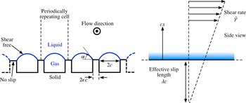
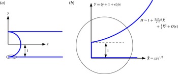
Schematic diagrams of the dimensional problem governing the effective slip length for longitudinal flow over a ‘bubble mattress’.

The paper proceeds as follows. In § 2 we formulate the problem. In § 3 we invoke an exact mathematical analogy between the effective-slip problem and that of ideal flow through a constricted slit channel (Crowdy Reference Crowdy2011a
), which facilitates a scaling analysis of the slip-length singularity. In §§ 4 and 5 we respectively analyse the cases
 $0\leqslant \unicode[STIX]{x1D6FC}<\unicode[STIX]{x03C0}/2$
and
 $0<\unicode[STIX]{x03C0}/2-\unicode[STIX]{x1D6FC}=O(\unicode[STIX]{x1D716}^{1/2})$
, which are the two distinguished small-
 $\unicode[STIX]{x1D716}$
limits identified in § 3. In § 6 we recapitulate the expansions found in the different regimes and combine them to form a uniformly valid approximation valid for arbitrary protrusion angles in the range
 $0\leqslant \unicode[STIX]{x1D6FC}\leqslant \unicode[STIX]{x03C0}/2$
; we also show comparisons of the asymptotic formulae with numerical data.
2 Problem formulation
Our interest is in the slip length for longitudinal flow over a ‘bubble mattress’ configuration, as shown in figure 1. The liquid domain is bounded from below by an interface compound of a periodic array of cylindrical bubble (‘shear-free’) protrusions and the flat solid (‘no-slip’) segments separating them. The period is
 $L=2c(1+\unicode[STIX]{x1D716})$
, where
 $2c$
is the planform length of the bubble protrusions and
 $\unicode[STIX]{x1D716}$
the planform solid-to-fluid fraction. Assuming the capillary number is small, the gas–liquid interface is approximated as fixed and circularly shaped; we consider protrusion angles in the range
 $0\leqslant \unicode[STIX]{x1D6FC}\leqslant \unicode[STIX]{x03C0}/2$
. Calculating the effective slip length entails solving for the unidirectional flow field parallel to the grooves that asymptotes at large distances to a simple shear flow (shear rate
 $\dot{\unicode[STIX]{x1D6FE}}$
). If
 $\dot{\unicode[STIX]{x1D6FE}}cw$
is the flow component parallel to the grooves and
 $cx$
is the distance from the surface (measured normal to the flat solid segments) then
 $w\sim x+\unicode[STIX]{x1D706}+o(1)$
as
 $x\rightarrow \infty$
, where
 $$\begin{eqnarray}\unicode[STIX]{x1D706}=\hat{\boldsymbol{e}}_{\Vert }\hat{\boldsymbol{e}}_{\Vert }\boldsymbol{ : }\unicode[STIX]{x1D740}/c\end{eqnarray}$$
is the longitudinal slip length normalised by the planform bubble radius
 $c$
.
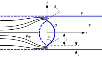
Dimensionless schematic of the elementary unit cell
 ${\mathcal{D}}$
. The longitudinal flow component
 $w$
can be extended to negative
 $x$
, with
 $w(-x,y)=w(x,y)$
; the extension reveals an analogy with ideal flow through a constricted slit channel where the dimensionless slip length
 $\unicode[STIX]{x1D706}$
is the counterpart of the blockage coefficient (Crowdy Reference Crowdy2011a
).

It is convenient to adopt a dimensionless formulation where lengths are normalised by
 $c$
and velocities by
 $\dot{\unicode[STIX]{x1D6FE}}c$
; we accordingly use the dimensionless Cartesian coordinates
 $(x,y)$
where
 $y$
is defined as shown in figure 2. Owing to the periodicity of the problem it suffices to consider a single ‘unit cell’
 ${\mathcal{D}}$
of dimensionless width
 $L/c=2(1+\unicode[STIX]{x1D716})$
bounded by the rays
 $$\begin{eqnarray}{\mathcal{P}}:\quad y=\pm (1+\unicode[STIX]{x1D716})\quad (x>0),\end{eqnarray}$$
the bubble interface
 $$\begin{eqnarray}{\mathcal{B}}:\quad (x+\cot \unicode[STIX]{x1D6FC})^{2}+y^{2}-(1+\cot ^{2}\unicode[STIX]{x1D6FC})=0\quad (x>0)\end{eqnarray}$$
and the flat solid boundaries
 $$\begin{eqnarray}{\mathcal{S}}:\quad 1<|y|<1+\unicode[STIX]{x1D716}\quad (x=0).\end{eqnarray}$$
The problem governing the longitudinal velocity component
 $w$
consists of Laplace’s equation
 $$\begin{eqnarray}\unicode[STIX]{x1D6FB}^{2}w=0\quad \text{in }{\mathcal{D}},\end{eqnarray}$$
the no-shear condition
 $$\begin{eqnarray}\frac{\unicode[STIX]{x2202}w}{\unicode[STIX]{x2202}n}=0\quad \text{on }{\mathcal{B}},\end{eqnarray}$$
the no-slip condition
 $$\begin{eqnarray}w=0\quad \text{on }{\mathcal{S}},\end{eqnarray}$$
the far-field condition
 $$\begin{eqnarray}w\sim x\quad \text{as }x\rightarrow \infty\end{eqnarray}$$
and periodic boundary conditions on
 ${\mathcal{P}}$
. Since
 $w(y)=w(-y)$
in
 ${\mathcal{D}}$
this periodicity can be enforced by the Neumann condition
 $$\begin{eqnarray}\frac{\unicode[STIX]{x2202}w}{\unicode[STIX]{x2202}y}=0\quad \text{on }{\mathcal{P}}.\end{eqnarray}$$
Our goal is to calculate the normalised slip length
 $$\begin{eqnarray}\unicode[STIX]{x1D706}(\unicode[STIX]{x1D716},\unicode[STIX]{x1D6FC})=\lim _{x\rightarrow \infty }(w-x)\end{eqnarray}$$
in the limit
 $\unicode[STIX]{x1D716}\rightarrow 0$
and for
 $0\leqslant \unicode[STIX]{x1D6FC}\leqslant \unicode[STIX]{x03C0}/2$
.
3 Ideal-flow analogy and scaling analysis
Integrating (2.5) over
 ${\mathcal{D}}$
and then applying the divergence theorem in the plane using (2.6) and (2.9) we find the integral relation
 $$\begin{eqnarray}\int _{1}^{1+\unicode[STIX]{x1D716}}\frac{\unicode[STIX]{x2202}w}{\unicode[STIX]{x2202}x}\,\text{d}y=1+\unicode[STIX]{x1D716}\quad \text{at }x=0.\end{eqnarray}$$
Physically, (3.1) represents the equivalence of the shear force away from the surface and that acting on its solid segments.
An alternative interpretation can be given based on a mathematically exact analogy between the slip problem formulated in § 2 and that of ideal flow through a constricted channel (Crowdy Reference Crowdy2011a
). The analogy is established by extending
 $w$
to negative
 $x$
such that
 $w(-x,y)=w(x,y)$
and defining a (fictitious) irrotational and incompressible flow
 $\unicode[STIX]{x1D735}w$
in the
 $xy$
plane (see figure 2). Relation (3.1) can then be interpreted as saying that, owing to symmetry and ‘impermeability’ of the boundaries
 ${\mathcal{B}}$
and
 ${\mathcal{P}}$
, half of the flux prescribed by (2.8) passes through each of the apertures
 ${\mathcal{S}}$
. As pointed out by Crowdy (Reference Crowdy2011a
), the dimensionless slip length
 $\unicode[STIX]{x1D706}$
is analogous to the so-called ‘blockage coefficient’ of the constricted channel, which measures the degree to which the flow is occluded by the constriction (whose boundary here is formed by
 ${\mathcal{B}}$
and its reflection about the
 $y$
axis). A similar analogy in the context of ohmic conduction relates
 $\unicode[STIX]{x1D706}$
to an ‘excess resistance’ (Yariv & Sherwood Reference Yariv and Sherwood2015).
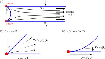
(a) The fictitious ideal flow
 $\unicode[STIX]{x1D735}w$
as seen on the
 $O(1)$
scale of the bubble/periodicity. (b,c) Continuity of the fictitious ideal flow
 $\unicode[STIX]{x1D735}w$
dictates the nature of the apparent flux singularity as
 $(x,y)$
approach
 $(0,\pm 1)$
, which are resolved at small distances from those points where the gap becomes discernible.

Clearly the blockage coefficient (and hence
 $\unicode[STIX]{x1D706}$
) should diverge in the limit
 $\unicode[STIX]{x1D716}\rightarrow 0$
as the apertures become exceedingly narrow. On the scale of the bubble (see figure 3
a) the apertures are indiscernible and the total flux through the channel is
 ${\approx}2$
(cf. (2.8)); the fictitious flow appears to be injected into
 ${\mathcal{D}}$
from two singular points
 $(x,y)\approx (0,\pm 1)$
.
Let us consider the nature of this singularity in the respective cases
 $0\leqslant \unicode[STIX]{x1D6FC}<\unicode[STIX]{x03C0}/2$
and
 $0<\unicode[STIX]{x03C0}/2-\unicode[STIX]{x1D6FC}\ll 1$
(see figure 3
b,c). Starting with the former case, if
 $r$
is the radial distance from
 $(x,y)\approx (0,-1)$
then for
 $\unicode[STIX]{x1D716}\ll r\ll 1$
the fluid boundaries appear to intersect at an acute angle
 $\unicode[STIX]{x03C0}/2-\unicode[STIX]{x1D6FC}$
and continuity dictates
 $$\begin{eqnarray}0\leqslant \unicode[STIX]{x1D6FC}<\unicode[STIX]{x03C0}/2:\quad \unicode[STIX]{x1D735}w\approx \frac{1}{\unicode[STIX]{x03C0}/2-\unicode[STIX]{x1D6FC}}\frac{1}{r}\hat{\boldsymbol{e}}_{r}\quad \text{for }\unicode[STIX]{x1D716}\ll r\ll 1,\end{eqnarray}$$
where
 $\hat{\boldsymbol{e}}_{r}$
is a unit vector in the radial direction. Integration gives
 $$\begin{eqnarray}0\leqslant \unicode[STIX]{x1D6FC}<\unicode[STIX]{x03C0}/2:\quad w\approx {\mathcal{C}}_{l}-\frac{1}{\unicode[STIX]{x03C0}/2-\unicode[STIX]{x1D6FC}}\ln \frac{1}{r}\quad \text{for }\unicode[STIX]{x1D716}\ll r\ll 1,\end{eqnarray}$$
wherein the fact that
 $w>0$
for
 $x>0$
requires bounding the order of magnitude of the integration constant
 ${\mathcal{C}}_{l}$
from below:
 $$\begin{eqnarray}{\mathcal{C}}_{l}\gtrsim O\left(\ln \frac{1}{\unicode[STIX]{x1D716}}\right).\end{eqnarray}$$
The singular behaviour (3.3) breaks down as
 $\unicode[STIX]{x1D6FC}\rightarrow \unicode[STIX]{x03C0}/2$
. To characterise the transition we note that for
 $\unicode[STIX]{x03C0}/2-\unicode[STIX]{x1D6FC}\ll 1$
the bubble boundary
 ${\mathcal{B}}$
near
 $(x,y)=(0,-1)$
can be approximated as (cf. (2.3))
 $$\begin{eqnarray}1+y\approx {\textstyle \frac{1}{2}}x^{2}+x(\unicode[STIX]{x03C0}/2-\unicode[STIX]{x1D6FC}),\end{eqnarray}$$
where the first term on the right-hand side is dominant for
 $\unicode[STIX]{x03C0}/2-\unicode[STIX]{x1D6FC}\ll x$
; the bubble boundary
 ${\mathcal{B}}$
is then approximately parabolic implying that the
 $O(\unicode[STIX]{x1D716})$
gaps are indiscernible for
 $x\gg \unicode[STIX]{x1D716}^{1/2}$
. It follows that if
 $\unicode[STIX]{x03C0}/2-\unicode[STIX]{x1D6FC}=O(\unicode[STIX]{x1D716}^{1/2})$
there exists an intermediate scale
 $\unicode[STIX]{x1D716}^{1/2}\ll x\ll 1$
where the bubble boundary appears parabolic yet the gaps are indiscernible. The flow thus appears to emanate from geometric cusp singularities and continuity accordingly dictates
 $$\begin{eqnarray}\unicode[STIX]{x03C0}/2-\unicode[STIX]{x1D6FC}=O(\unicode[STIX]{x1D716}^{1/2}):\quad \unicode[STIX]{x1D735}w\approx \frac{2}{x^{2}}\hat{\boldsymbol{e}}_{x}\quad \text{for }\unicode[STIX]{x1D716}^{1/2}\ll x\ll 1,\end{eqnarray}$$
where
 $\hat{\boldsymbol{e}}_{x}$
is a unit vector along the
 $x$
axis. Integrating and applying the same positivity argument as before we find that
 $$\begin{eqnarray}\unicode[STIX]{x03C0}/2-\unicode[STIX]{x1D6FC}=O(\unicode[STIX]{x1D716}^{1/2}):\quad w\approx {\mathcal{C}}_{a}-\frac{2}{x}\quad \text{for }\unicode[STIX]{x1D716}^{1/2}\ll x\ll 1,\end{eqnarray}$$
where
 $$\begin{eqnarray}{\mathcal{C}}_{a}\gtrsim O\left(\unicode[STIX]{x1D716}^{-1/2}\right).\end{eqnarray}$$
To pin down the scalings of the constants
 ${\mathcal{C}}_{l}$
and
 ${\mathcal{C}}_{a}$
we note that the singular expansions (3.3) and (3.7) break down at sufficiently small
 $x$
once the gap becomes discernible. The integral relation (3.1) suggests that to compensate for the narrowness of the aperture the normal ideal-flow component
 $\unicode[STIX]{x2202}w/\unicode[STIX]{x2202}x$
at
 $x=0$
must be
 $O(1/\unicode[STIX]{x1D716})$
as
 $\unicode[STIX]{x1D716}\rightarrow 0$
. Thus
 $w=O(\unicode[STIX]{x0394}x/\unicode[STIX]{x1D716})$
, where
 $\unicode[STIX]{x0394}x$
represents the length scale on which
 $w$
varies near the aperture; the above discussion implies that
 $\unicode[STIX]{x0394}x=O(\unicode[STIX]{x1D716})$
for
 $0\leqslant \unicode[STIX]{x1D6FC}<\unicode[STIX]{x03C0}/2$
and
 $O(\unicode[STIX]{x1D716}^{1/2})$
for
 $\unicode[STIX]{x03C0}/2-\unicode[STIX]{x1D6FC}=O(\unicode[STIX]{x1D716}^{1/2})$
. Hence, for
 $x=O(\unicode[STIX]{x0394}x)$
,
 $$\begin{eqnarray}w=\left\{\begin{array}{@{}ll@{}}O(1),\quad & 0\leqslant \unicode[STIX]{x1D6FC}<\unicode[STIX]{x03C0}/2,\\ O(\unicode[STIX]{x1D716}^{-1/2}),\quad & \unicode[STIX]{x03C0}/2-\unicode[STIX]{x1D6FC}=O(\unicode[STIX]{x1D716}^{1/2}).\end{array}\right.\end{eqnarray}$$
These orders of magnitude must however be compatible with (3.3) and (3.7), which in light of (3.4) and (3.8) is only possible if
 $$\begin{eqnarray}{\mathcal{C}}_{l}=\frac{1}{\unicode[STIX]{x03C0}/2-\unicode[STIX]{x1D6FC}}\ln \frac{1}{\unicode[STIX]{x1D716}}+O(1),\quad {\mathcal{C}}_{a}=O(\unicode[STIX]{x1D716}^{-1/2}).\end{eqnarray}$$
Let us now return to the fictitious ideal flow
 $\unicode[STIX]{x1D735}w$
as it is perceived on the scale of the periodicity (figure 3
a). Ignoring small corrections, this flow is uniquely determined by the prescribed fluxes from the singular points
 $(x,y)\approx (0,\pm 1)$
. In contrast,
 $w$
is determined by this prescription only up to an additive constant, leaving the effective slip length
 $\unicode[STIX]{x1D706}$
undetermined. In principal we could (and later will) proceed by calculating
 ${\mathcal{C}}_{l/a}$
from local solutions in the vicinities of the apertures. For scaling purposes, however, it is sufficient to note that the differences
 $\unicode[STIX]{x1D706}-{\mathcal{C}}_{l/a}$
are uniquely determined by the degenerate ideal-flow problem, which is independent of
 $\unicode[STIX]{x1D716}$
. It follows that
 $\unicode[STIX]{x1D706}\sim {\mathcal{C}}_{l/a}+O(1)$
and together with (3.10) we find
 $$\begin{eqnarray}\unicode[STIX]{x1D706}\sim \left\{\begin{array}{@{}ll@{}}\displaystyle \frac{1}{\unicode[STIX]{x03C0}/2-\unicode[STIX]{x1D6FC}}\ln \frac{1}{\unicode[STIX]{x1D716}}+O(1),\quad & 0\leqslant \unicode[STIX]{x1D6FC}<\unicode[STIX]{x03C0}/2,\\ O(\unicode[STIX]{x1D716}^{-1/2}),\quad & \unicode[STIX]{x03C0}/2-\unicode[STIX]{x1D6FC}=O(\unicode[STIX]{x1D716}^{1/2}).\end{array}\right.\end{eqnarray}$$
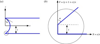
The leading-order fluid boundaries in the outer (a) and inner (b) limits for
 $0\leqslant \unicode[STIX]{x1D6FC}<\unicode[STIX]{x03C0}/2$
where
 $\unicode[STIX]{x03C0}/2-\unicode[STIX]{x1D6FC}=O(1)$
.

Note that (3.11) is consistent with both Philip’s solution (1.2) for
 $\unicode[STIX]{x1D6FC}=0$
and the asymptotic expansion (1.3) for
 $\unicode[STIX]{x1D6FC}=\unicode[STIX]{x03C0}/2$
. The scaling analysis explicitly predicts how the leading logarithmic term in Philip’s solution generalises to positive
 $\unicode[STIX]{x1D6FC}$
(not too close to
 $\unicode[STIX]{x03C0}/2$
). It also quantifies the robustness of the inverse-square-root scaling to deviations of
 $\unicode[STIX]{x1D6FC}$
from
 $\unicode[STIX]{x03C0}/2$
.
In what follows we carry out a more rigorous and detailed asymptotic analysis of the two distinguished protrusion-angle regimes, which will lead to explicit expansions up to an error that is
 $o(1)$
as
 $\unicode[STIX]{x1D716}\rightarrow 0$
. Readers not interested in the mathematical details of the derivation may wish to skip to § 6, where the expansions are discussed and used to form a uniformly valid approximation for arbitrary protrusion angles.
4 Arbitrary protrusion angles
 $0\leqslant \unicode[STIX]{x1D6FC}<\unicode[STIX]{x03C0}/2$

Thus we turn to a more detailed asymptotic study, starting with protrusion angles
 $0\leqslant \unicode[STIX]{x1D6FC}<\unicode[STIX]{x03C0}/2$
with
 $\unicode[STIX]{x03C0}/2-\unicode[STIX]{x1D6FC}=O(1)$
. Following (3.11) we assume the slip-length expansion
 $$\begin{eqnarray}\unicode[STIX]{x1D706}\sim \frac{1}{\unicode[STIX]{x03C0}/2-\unicode[STIX]{x1D6FC}}\ln \frac{1}{\unicode[STIX]{x1D716}}+\unicode[STIX]{x1D706}_{0}+o(1)\quad \text{as }\unicode[STIX]{x1D716}\rightarrow 0,\end{eqnarray}$$
our goal being to determine
 $\unicode[STIX]{x1D706}_{0}(\unicode[STIX]{x1D6FC})$
. The intuitive picture of § 3 suggests that the asymptotic behaviour of
 $w$
is spatially non-uniform. There are two distinguished limits to consider (see figure 4): the ‘outer’ limit
 $\unicode[STIX]{x1D716}\rightarrow 0$
with
 $(x,y)$
fixed, which represents the flow as perceived on the scale of the periodicity; and the ‘inner’ limits
 $\unicode[STIX]{x1D716}\rightarrow 0$
with
 $(x,y\pm 1)=O(\unicode[STIX]{x1D716})$
.
In the outer region expansion (4.1) suggests
 $$\begin{eqnarray}w\sim w_{l}(x,y)\ln \frac{1}{\unicode[STIX]{x1D716}}+w_{0}(x,y)+o(1)\quad \text{as }\unicode[STIX]{x1D716}\rightarrow 0\quad \text{with }(x,y)\text{ fixed}.\end{eqnarray}$$
Inspecting the formulation in § 2, both
 $w_{l}$
and
 $w_{0}$
satisfy Laplace’s equation in the degenerate curvilinear triangle domain bounded by the rays
 $y=\pm 1$
(
 $x>0$
) and the semi-circle
 ${\mathcal{B}}$
, along with Neumann conditions on the boundaries of this domain. At large distances,
 $$\begin{eqnarray}w_{l}\sim \frac{1}{\unicode[STIX]{x03C0}/2-\unicode[STIX]{x1D6FC}}+o(1),\quad w_{0}\sim x+\unicode[STIX]{x1D706}_{0}+o(1)\quad \text{as }x\rightarrow \infty .\end{eqnarray}$$
At
 $(x,y)=(0,\pm 1)$
the outer geometry is singular, the rays
 $y=\pm 1$
and
 ${\mathcal{B}}$
meeting at an acute
 $\unicode[STIX]{x03C0}/2-\unicode[STIX]{x1D6FC}$
angle. The discussion in § 3 suggests the leading-order behaviours
 $$\begin{eqnarray}w_{l}\sim \frac{1}{\unicode[STIX]{x03C0}/2-\unicode[STIX]{x1D6FC}},\quad w_{0}\sim \frac{1}{\unicode[STIX]{x03C0}/2-\unicode[STIX]{x1D6FC}}\ln \sqrt{x^{2}+(y\mp 1)^{2}}\quad \text{as }(x,y)\rightarrow (0,\pm 1),\end{eqnarray}$$
which we shall later verify by matching with the inner regions. The first of these conditions shows that
 $w_{l}$
is constant,
 $$\begin{eqnarray}w_{l}=\frac{1}{\unicode[STIX]{x03C0}/2-\unicode[STIX]{x1D6FC}}.\end{eqnarray}$$
The second closes the problem governing
 $w_{0}$
up to an additive constant, which can only be found by matching with the inner regions. Owing to this additive freedom,
 $\unicode[STIX]{x1D706}_{0}$
remains unknown; the difference
 $w_{0}-\unicode[STIX]{x1D706}_{0}$
is, however, uniquely determined and in appendix A we find
 $$\begin{eqnarray}w_{0}-\unicode[STIX]{x1D706}_{0}\sim \frac{1}{\unicode[STIX]{x03C0}/2-\unicode[STIX]{x1D6FC}}\ln \sqrt{x^{2}+(y\mp 1)^{2}}-\mathscr{B}_{o}(\unicode[STIX]{x1D6FC})+o(1)\quad \text{as }(x,y)\rightarrow (0,\pm 1),\end{eqnarray}$$
where
 $$\begin{eqnarray}\displaystyle \mathscr{B}_{o}(\unicode[STIX]{x1D6FC}) & = & \displaystyle \frac{1}{\unicode[STIX]{x03C0}/2-\unicode[STIX]{x1D6FC}}\ln \frac{2\cot \unicode[STIX]{x1D6FC}\,\unicode[STIX]{x1D6E4}(1-\unicode[STIX]{x1D6FC}/\unicode[STIX]{x03C0})\unicode[STIX]{x1D6E4}(1/2+\unicode[STIX]{x1D6FC}/\unicode[STIX]{x03C0})}{\unicode[STIX]{x1D6E4}(\unicode[STIX]{x1D6FC}/\unicode[STIX]{x03C0})\unicode[STIX]{x1D6E4}(3/2-\unicode[STIX]{x1D6FC}/\unicode[STIX]{x03C0})}\nonumber\\ \displaystyle & & \displaystyle +\,2\cot \unicode[STIX]{x1D6FC}-\frac{2}{\unicode[STIX]{x03C0}}\ln 4+\frac{2}{\unicode[STIX]{x03C0}}\unicode[STIX]{x1D6FE}_{E}+\frac{2}{\unicode[STIX]{x03C0}}\unicode[STIX]{x1D713}(\unicode[STIX]{x1D6FC}/\unicode[STIX]{x03C0}).\end{eqnarray}$$
In (4.7)
 $\unicode[STIX]{x1D6E4}$
is the gamma function,
 $\unicode[STIX]{x1D713}=\unicode[STIX]{x1D6E4}^{\prime }/\unicode[STIX]{x1D6E4}$
the digamma function and
 $\unicode[STIX]{x1D6FE}_{E}\approx 0.5772$
the Euler–Mascheroni constant.
Consider now the inner region where the stretched coordinates
 $$\begin{eqnarray}Y=(y+1+\unicode[STIX]{x1D716})/\unicode[STIX]{x1D716},\quad X=x/\unicode[STIX]{x1D716}\end{eqnarray}$$
are
 $O(1)$
(from symmetry it suffices to consider
 $y<0$
) and the bubble boundary is
 $Y\sim 1+X\cot \unicode[STIX]{x1D6FC}+o(1)$
. From § 3 we anticipate the expansion
 $$\begin{eqnarray}w\sim W_{0}(X,Y)+o(1),\end{eqnarray}$$
where
 $W_{0}=O(1)$
is governed by Laplace’s equation
 $$\begin{eqnarray}\frac{\unicode[STIX]{x2202}^{2}W_{0}}{\unicode[STIX]{x2202}X^{2}}+\frac{\unicode[STIX]{x2202}^{2}W_{0}}{\unicode[STIX]{x2202}Y^{2}}=0,\end{eqnarray}$$
the Dirichlet condition
 $$\begin{eqnarray}W_{0}=0\quad \text{at }X=0\end{eqnarray}$$
and the Neumann conditions
 $$\begin{eqnarray}\frac{\unicode[STIX]{x2202}W_{0}}{\unicode[STIX]{x2202}N}=0\quad \text{at }Y=0\quad \text{and}\quad 1+X\cot \unicode[STIX]{x1D6FC},\end{eqnarray}$$
where
 $\unicode[STIX]{x2202}/\unicode[STIX]{x2202}N$
respectively denotes differentiation in a direction normal to the cell boundary
 $Y=0$
and the nominal bubble boundary
 $Y=1+X\cot \unicode[STIX]{x1D6FC}$
. On the one hand, asymptotic matching with the outer region dictates the far-field behaviour
 $$\begin{eqnarray}W_{0}\sim \frac{1}{\unicode[STIX]{x03C0}/2-\unicode[STIX]{x1D6FC}}\ln \sqrt{X^{2}+Y^{2}}+\unicode[STIX]{x1D706}_{0}-\mathscr{B}_{o}(\unicode[STIX]{x1D6FC})+o(1)\quad \text{as }X^{2}+Y^{2}\rightarrow \infty .\end{eqnarray}$$
On the other hand,
 $W_{0}$
is fully determined by the leading logarithmic term in (4.13); in fact, in appendix B we find
 $$\begin{eqnarray}W_{0}\sim \frac{1}{\unicode[STIX]{x03C0}/2-\unicode[STIX]{x1D6FC}}\ln \sqrt{X^{2}+Y^{2}}+\mathscr{B}_{i}(\unicode[STIX]{x1D6FC})+o(1)\quad \text{as }X^{2}+Y^{2}\rightarrow \infty ,\end{eqnarray}$$
where
 $$\begin{eqnarray}\mathscr{B}_{i}(\unicode[STIX]{x1D6FC})=\frac{1}{\unicode[STIX]{x03C0}/2-\unicode[STIX]{x1D6FC}}\ln \frac{2^{1-2\unicode[STIX]{x1D6FC}/\unicode[STIX]{x03C0}}(1/2-\unicode[STIX]{x1D6FC}/\unicode[STIX]{x03C0})\sqrt{\unicode[STIX]{x03C0}}}{\unicode[STIX]{x1D6E4}(3/2-\unicode[STIX]{x1D6FC}/\unicode[STIX]{x03C0})/\unicode[STIX]{x1D6E4}(1-\unicode[STIX]{x1D6FC}/\unicode[STIX]{x03C0})}.\end{eqnarray}$$
Clearly, expansions (4.13) and (4.14) must agree, hence
 $$\begin{eqnarray}\unicode[STIX]{x1D706}_{0}=\mathscr{B}_{i}(\unicode[STIX]{x1D6FC})+\mathscr{B}_{o}(\unicode[STIX]{x1D6FC}).\end{eqnarray}$$
5 Protrusion angles
$\unicode[STIX]{x03C0}/2-\unicode[STIX]{x1D6FC}=O(\unicode[STIX]{x1D716}^{1/2})$

In this regime the scaling analysis of § 3 suggests the slip-length expansion
 $$\begin{eqnarray}\unicode[STIX]{x1D706}\sim \unicode[STIX]{x1D716}^{-1/2}\unicode[STIX]{x1D706}_{-1/2}+\unicode[STIX]{x1D706}_{0}+o(1)\quad \text{as }\unicode[STIX]{x1D716}\rightarrow 0.\end{eqnarray}$$
We further inferred that near
 $x=0$
the field
 $w=O(\unicode[STIX]{x1D716}^{-1/2})$
and varies rapidly over a
 $O(\unicode[STIX]{x1D716}^{1/2})$
length scale. This suggests starting from the inner region, now defined as the region where the modified stretched coordinates
 $$\begin{eqnarray}\bar{X}=x/\unicode[STIX]{x1D716}^{1/2},\quad Y=(y+1+\unicode[STIX]{x1D716})/\unicode[STIX]{x1D716}\end{eqnarray}$$
are
 $O(1)$
. With this rescaling the bubble surface becomes
 $$\begin{eqnarray}Y=H(\bar{X})\sim H_{0}(\bar{X})+O(\unicode[STIX]{x1D716}),\quad H_{0}(\bar{X})=1+\unicode[STIX]{x1D70F}\bar{X}+\frac{\bar{X}^{2}}{2},\end{eqnarray}$$
where
 $$\begin{eqnarray}\unicode[STIX]{x1D70F}=(\unicode[STIX]{x03C0}/2-\unicode[STIX]{x1D6FC})/\unicode[STIX]{x1D716}^{1/2}\end{eqnarray}$$
is an
 $O(1)$
parameter. Defining
 $w(x,y)=W(X,Y)$
we find from (2.5)–(2.7) and (2.9) the problem:
 $$\begin{eqnarray}\displaystyle & \displaystyle \unicode[STIX]{x1D716}\frac{\unicode[STIX]{x2202}^{2}W}{\unicode[STIX]{x2202}\bar{X}^{2}}+\frac{\unicode[STIX]{x2202}^{2}W}{\unicode[STIX]{x2202}Y^{2}}=0\quad \text{for }\bar{X}>0,~0<Y<H(\bar{X}), & \displaystyle\end{eqnarray}$$
 $$\begin{eqnarray}\displaystyle & \displaystyle W=0\quad \text{at }\bar{X}=0, & \displaystyle\end{eqnarray}$$
 $$\begin{eqnarray}\displaystyle & \displaystyle \frac{\unicode[STIX]{x2202}W}{\unicode[STIX]{x2202}Y}=0\quad \text{at }Y=0, & \displaystyle\end{eqnarray}$$
 $$\begin{eqnarray}\displaystyle & \displaystyle \frac{\unicode[STIX]{x2202}W}{\unicode[STIX]{x2202}Y}-\unicode[STIX]{x1D716}\frac{\text{d}H}{\text{d}\bar{X}}\frac{\unicode[STIX]{x2202}W}{\unicode[STIX]{x2202}\bar{X}}=0\quad \text{at }Y=H(\bar{X}), & \displaystyle\end{eqnarray}$$
to be considered in conjunction with asymptotic matching as
 $\bar{X}\rightarrow \infty$
. To minimise going back and forth between the inner and outer regions we shall take advantage of the integral relation (3.1), which we rewrite here as
 $$\begin{eqnarray}\unicode[STIX]{x1D716}^{1/2}\int _{0}^{1}\frac{\unicode[STIX]{x2202}W}{\unicode[STIX]{x2202}\bar{X}}\,\text{d}Y=1+\unicode[STIX]{x1D716}\quad \text{at }\bar{X}=0.\end{eqnarray}$$
We now expand
 $W$
as
 $$\begin{eqnarray}W=\unicode[STIX]{x1D716}^{-1/2}W_{-1/2}+W_{0}+\unicode[STIX]{x1D716}^{1/2}W_{1/2}+\unicode[STIX]{x1D716}W_{1}+\cdots \,,\end{eqnarray}$$
where it is readily seen that the two leading terms are independent of
 $Y$
, i.e.
 $W_{-1/2}=W_{-1/2}(\bar{X})$
and
 $W_{0}=W_{0}(\bar{X})$
. From (5.6) and (5.9), these functions satisfy
 $$\begin{eqnarray}\displaystyle & \displaystyle W_{-1/2}=0,\quad \frac{\text{d}W_{-1/2}}{\text{d}\bar{X}}=1\quad \text{at }\bar{X}=0, & \displaystyle\end{eqnarray}$$
 $$\begin{eqnarray}\displaystyle & \displaystyle W_{0}=0,\quad \frac{\text{d}W_{0}}{\text{d}\bar{X}}=0\quad \text{at }\bar{X}=0. & \displaystyle\end{eqnarray}$$
Differential equations governing
 $W_{-1/2}$
and
 $W_{0}$
arise as solvability conditions on the higher-order terms
 $W_{1/2}$
and
 $W_{1}$
. From (5.5), (5.7) and (5.8) the latter satisfy:
 $$\begin{eqnarray}\displaystyle & \displaystyle \frac{\unicode[STIX]{x2202}^{2}W_{1/2}}{\unicode[STIX]{x2202}Y^{2}}=-\frac{\text{d}^{2}W_{-1/2}}{\text{d}\bar{X}^{2}},\quad \frac{\unicode[STIX]{x2202}^{2}W_{1}}{\unicode[STIX]{x2202}Y^{2}}=-\frac{\text{d}^{2}W_{0}}{\text{d}\bar{X}^{2}}, & \displaystyle\end{eqnarray}$$
 $$\begin{eqnarray}\displaystyle & \displaystyle \frac{\unicode[STIX]{x2202}W_{1/2}}{\unicode[STIX]{x2202}Y}=0,\quad \frac{\unicode[STIX]{x2202}W_{1}}{\unicode[STIX]{x2202}Y}=0\quad \text{at }\bar{Y}=0, & \displaystyle\end{eqnarray}$$
 $$\begin{eqnarray}\displaystyle & \displaystyle \frac{\unicode[STIX]{x2202}W_{1/2}}{\unicode[STIX]{x2202}Y}=\frac{\text{d}H_{0}}{\text{d}\bar{X}}\frac{\text{d}W_{-1/2}}{\text{d}\bar{X}},\quad \frac{\unicode[STIX]{x2202}W_{1}}{\unicode[STIX]{x2202}Y}=\frac{\text{d}H_{0}}{\text{d}\bar{X}}\frac{\text{d}W_{0}}{\text{d}\bar{X}}\quad \text{at }Y=H_{0}(\bar{X}). & \displaystyle\end{eqnarray}$$
Note that in (5.15) we asymptotically mapped condition (5.8) to the nominal boundary
 $H_{0}(\bar{X})$
by means of a Taylor expansion (since
 $W_{-1/2}$
and
 $W_{0}$
are independent of
 $Y$
no additional terms arise at these orders). Through integration of (5.13) from
 $Y=0$
to
 $H_{0}(\bar{X})$
and making use of (5.14) and (5.15) we find
 $$\begin{eqnarray}\frac{\text{d}}{\text{d}\bar{X}}\left(H_{0}\frac{\text{d}W_{-1/2}}{\text{d}\bar{X}}\right)=0,\quad \frac{\text{d}}{\text{d}\bar{X}}\left(H_{0}\frac{\text{d}W_{0}}{\text{d}\bar{X}}\right)=0.\end{eqnarray}$$
The fields
 $W_{-1/2}$
and
 $W_{0}$
are determined by (5.16) together with the four conditions (5.11) applying at
 $X=0$
. It is readily seen that
 $$\begin{eqnarray}W_{0}\equiv 0;\end{eqnarray}$$
from the solution for
 $W_{-1/2}$
we only require the far-field behaviour
 $$\begin{eqnarray}W_{-1/2}\sim \frac{2\,\text{acosh}(\unicode[STIX]{x1D70F}/\sqrt{2})}{(\unicode[STIX]{x1D70F}^{2}-2)^{1/2}}-\frac{2}{\bar{X}}+O\left(\frac{1}{\bar{X}^{2}}\right)\quad \text{as }\bar{X}\rightarrow \infty ,\end{eqnarray}$$
where the branches of the square root and inverse hyperbolic functions are such that
 $$\begin{eqnarray}\frac{2\,\text{acosh}(\unicode[STIX]{x1D70F}/\sqrt{2})}{(\unicode[STIX]{x1D70F}^{2}-2)^{1/2}}=\left\{\begin{array}{@{}ll@{}}\displaystyle \frac{2}{\sqrt{2-\unicode[STIX]{x1D70F}^{2}}}\text{atan}\frac{\sqrt{2-\unicode[STIX]{x1D70F}^{2}}}{\unicode[STIX]{x1D70F}}\quad & 0<\unicode[STIX]{x1D70F}<\sqrt{2},\\ \displaystyle \sqrt{2}\quad & \unicode[STIX]{x1D70F}=\sqrt{2},\\ \displaystyle \frac{2}{\sqrt{\unicode[STIX]{x1D70F}^{2}-2}}\ln \left(\frac{\unicode[STIX]{x1D70F}}{\sqrt{2}}+\sqrt{\frac{\unicode[STIX]{x1D70F}^{2}}{2}-1}\right)\quad & \unicode[STIX]{x1D70F}>\sqrt{2}.\end{array}\right.\end{eqnarray}$$
The leading-order fluid boundaries in the outer (a) and inner (b) limits for
 $\unicode[STIX]{x03C0}/2-\unicode[STIX]{x1D6FC}=O(\unicode[STIX]{x1D716}^{1/2})$
.

We now turn to the outer limit
 $\unicode[STIX]{x1D716}\rightarrow 0$
with
 $(x,y)$
fixed. The fluid boundary is to leading order a degenerate zero-angle curvilinear triangle (see figure 5), the difference from the exact boundary being
 $O(\unicode[STIX]{x1D716}^{1/2})$
. Inspecting the inner terms (5.17) and (5.18) we deduce an outer expansion in the form
 $$\begin{eqnarray}w\sim \unicode[STIX]{x1D716}^{-1/2}\unicode[STIX]{x1D706}_{-1/2}+w_{0}(x,y)+\cdots \,,\end{eqnarray}$$
where
 $$\begin{eqnarray}\unicode[STIX]{x1D706}_{-1/2}=\frac{2\,\text{acosh}(\unicode[STIX]{x1D70F}/\sqrt{2})}{(\unicode[STIX]{x1D70F}^{2}-2)^{1/2}}.\end{eqnarray}$$
The field
 $w_{0}$
satisfies Laplace’s equation subject to homogeneous Neumann conditions on the leading-order outer boundary, the far-field condition
 $$\begin{eqnarray}w_{0}\sim x\quad \text{as }x\rightarrow \infty ,\end{eqnarray}$$
and the matching condition
 $$\begin{eqnarray}w_{0}\sim -\frac{2}{x}\quad \text{as }(x,y)\rightarrow (0,\pm 1).\end{eqnarray}$$
The above problem determines
 $w_{0}$
only up to an arbitrary additive constant, which can be taken to be
 $\unicode[STIX]{x1D706}_{0}=\lim _{x\rightarrow \infty }(w_{0}-x)$
. The problem has already been solved in Schnitzer (Reference Schnitzer2016), and from the solution we can extract the asymptotic behaviour
 $$\begin{eqnarray}w_{0}-\unicode[STIX]{x1D706}_{0}\sim -\frac{2}{x}+\frac{12}{\unicode[STIX]{x03C0}}\ln 2+o(1)\quad \text{as }(x,y)\rightarrow (0,\pm 1).\end{eqnarray}$$
Asymptotic matching with the inner fields (5.17) and (5.18) shows that
 $w_{0}$
cannot have an
 $O(1)$
term in the limit
 $(x,y)\rightarrow (0,\pm 1)$
. Thus (5.24) yields
 $$\begin{eqnarray}\unicode[STIX]{x1D706}_{0}=-\frac{12}{\unicode[STIX]{x03C0}}\ln 2.\end{eqnarray}$$
6 Discussion
6.1 Recapitulation
It is useful at this point to recapitulate the asymptotic expansions obtained in the different protrusion-angle regimes. First, from the analysis of § 4 we have
 $$\begin{eqnarray}0\leqslant \unicode[STIX]{x1D6FC}<\unicode[STIX]{x03C0}/2:\quad \unicode[STIX]{x1D706}\sim \frac{1}{\unicode[STIX]{x03C0}/2-\unicode[STIX]{x1D6FC}}\ln \frac{1}{\unicode[STIX]{x1D716}}+\mathscr{B}_{i}(\unicode[STIX]{x1D6FC})+\mathscr{B}_{o}(\unicode[STIX]{x1D6FC})+O(\unicode[STIX]{x1D716})\quad \text{as }\unicode[STIX]{x1D716}\rightarrow 0,\end{eqnarray}$$
where
 $\mathscr{B}_{o}$
and
 $\mathscr{B}_{i}$
are respectively provided by (4.7) and (4.15). For
 $\unicode[STIX]{x03C0}/2-\unicode[STIX]{x1D6FC}=O(1)$
the error estimate is found by considering higher-order terms (the error may be at most logarithmically larger than
 $O(\unicode[STIX]{x1D716})$
). Alluding to the ideal-flow analogy of § 3 we can interpret each of the three terms in (6.1) as blockage coefficients, where
 ${\mathcal{B}}_{i}$
accounts for the inner region,
 ${\mathcal{B}}_{o}$
for the outer region and the leading logarithmic term for the excess contribution of the overlap between these two regions.
Next, from the analysis of § 5 we have
 $$\begin{eqnarray}\displaystyle & \displaystyle \unicode[STIX]{x03C0}/2-\unicode[STIX]{x1D6FC}=O(\unicode[STIX]{x1D716}^{1/2}):\quad \unicode[STIX]{x1D706}\sim \frac{2\,\text{acosh}((\unicode[STIX]{x03C0}/2-\unicode[STIX]{x1D6FC})/\sqrt{2\unicode[STIX]{x1D716}})}{\left[(\unicode[STIX]{x03C0}/2-\unicode[STIX]{x1D6FC})^{2}-2\unicode[STIX]{x1D716}\right]^{1/2}}-\frac{12}{\unicode[STIX]{x03C0}}\ln 2+O(\unicode[STIX]{x1D716}^{1/2})\quad \text{as }\unicode[STIX]{x1D716}\rightarrow 0, & \displaystyle \nonumber\\ \displaystyle & & \displaystyle\end{eqnarray}$$
where note that the first term is
 $O(\unicode[STIX]{x1D716}^{-1/2})$
(cf. (5.19)). In contrast to (6.1), in (6.2) the dominant contribution arises solely from the inner region. In the context of the ideal-flow analogy, the first and second terms in (6.2) can be respectively interpreted as isolated inner and outer contributions to the blockage coefficient.
There is a third distinguished limit,
 $\unicode[STIX]{x03C0}/2-\unicode[STIX]{x1D6FC}=O(\unicode[STIX]{x1D716})$
, which we have tacitly ignored. A detailed analysis, which closely follows that for
 $\unicode[STIX]{x1D6FC}=\unicode[STIX]{x03C0}/2$
(Schnitzer Reference Schnitzer2016), shows that
 $$\begin{eqnarray}\unicode[STIX]{x03C0}/2-\unicode[STIX]{x1D6FC}=O(\unicode[STIX]{x1D716}):\quad \unicode[STIX]{x1D706}\sim \frac{\unicode[STIX]{x03C0}}{\sqrt{2\unicode[STIX]{x1D716}}}-\frac{12}{\unicode[STIX]{x03C0}}\ln 2-\frac{\unicode[STIX]{x03C0}/2-\unicode[STIX]{x1D6FC}}{\unicode[STIX]{x1D716}}+o(1)\quad \text{as }\unicode[STIX]{x1D716}\rightarrow 0.\end{eqnarray}$$
The same expansion is obtained however by taking the small
 $\unicode[STIX]{x1D70F}=(\unicode[STIX]{x03C0}/2-\unicode[STIX]{x1D6FC})/\unicode[STIX]{x1D716}^{1/2}$
limit of (6.2). Hence at least up to an
 $o(1)$
error (6.3) is included in (6.2). Note that for
 $\unicode[STIX]{x1D6FC}=\unicode[STIX]{x03C0}/2$
(6.3) is consistent with (1.3).
The normalised slip length
 $\unicode[STIX]{x1D706}$
as a function of the solid-fraction
 $\unicode[STIX]{x1D716}$
. The data symbols are numerical results (rectangles:
 $\unicode[STIX]{x1D6FC}=\unicode[STIX]{x03C0}/6$
, circles:
 $\unicode[STIX]{x1D6FC}=\unicode[STIX]{x03C0}/3$
, triangles:
 $\unicode[STIX]{x1D6FC}=\unicode[STIX]{x03C0}/2$
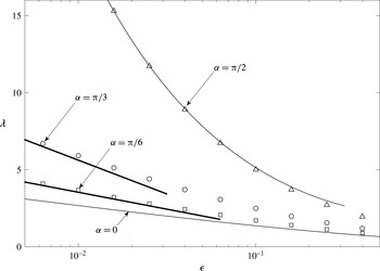
). The thick black lines are the asymptotic formula (6.1) for
 $0\leqslant \unicode[STIX]{x1D6FC}<\unicode[STIX]{x03C0}/2$
, the lower thin line is Philip’s solution (1.2) for
 $\unicode[STIX]{x1D6FC}=0$
and the upper thin line is the asymptotic expansion (1.3) for
 $\unicode[STIX]{x1D6FC}=\unicode[STIX]{x03C0}/2$
.

6.2 A uniformly valid approximation
There is an intermediate regime of protrusion angles where expansions (6.1) and (6.2) overlap. On the one hand, expanding (6.2) for
 $\unicode[STIX]{x03C0}/2-\unicode[STIX]{x1D6FC}\gg \unicode[STIX]{x1D716}^{1/2}$
gives
 $$\begin{eqnarray}\quad \unicode[STIX]{x1D706}\approx \frac{1}{\unicode[STIX]{x03C0}/2-\unicode[STIX]{x1D6FC}}\ln \frac{2(\unicode[STIX]{x03C0}/2-\unicode[STIX]{x1D6FC})^{2}}{\unicode[STIX]{x1D716}}-\frac{12}{\unicode[STIX]{x03C0}}\ln 2+O[(\unicode[STIX]{x03C0}/2-\unicode[STIX]{x1D6FC})^{-3}\unicode[STIX]{x1D716}],\end{eqnarray}$$
the error being
 $o(1)$
for
 $\unicode[STIX]{x1D716}^{1/3}\ll \unicode[STIX]{x03C0}/2-\unicode[STIX]{x1D6FC}\ll 1$
. On the other hand, expanding (6.1) for
 $\unicode[STIX]{x03C0}/2-\unicode[STIX]{x1D6FC}\ll 1$
yields the two terms as in (6.4), with an error that is
 $O(\unicode[STIX]{x03C0}/2-\unicode[STIX]{x1D6FC})$
. Hence, for
 $\unicode[STIX]{x1D716}^{1/3}\ll \unicode[STIX]{x03C0}/2-\unicode[STIX]{x1D6FC}\ll 1$
expansions (6.1) and (6.2) are asymptotically identical up to an
 $o(1)$
error. Adding the two expansions and subtracting their overlap yields the uniformly valid approximation
 $$\begin{eqnarray}\unicode[STIX]{x1D706}\approx \frac{2\cosh ^{-1}\left[(\unicode[STIX]{x03C0}/2-\unicode[STIX]{x1D6FC})/\sqrt{2\unicode[STIX]{x1D716}}\right]}{\left[(\unicode[STIX]{x03C0}/2-\unicode[STIX]{x1D6FC})^{2}-2\unicode[STIX]{x1D716}\right]^{1/2}}-\frac{1}{\unicode[STIX]{x03C0}/2-\unicode[STIX]{x1D6FC}}\ln \left[2(\unicode[STIX]{x03C0}/2-\unicode[STIX]{x1D6FC})^{2}\right]+\mathscr{B}_{i}(\unicode[STIX]{x1D6FC})+\mathscr{B}_{o}(\unicode[STIX]{x1D6FC}),\end{eqnarray}$$
whose error is
 $o(1)$
for all protrusion angles
 $0\leqslant \unicode[STIX]{x1D6FC}\leqslant \unicode[STIX]{x03C0}/2$
.
6.3 Comparison with numerical data
We here compare our asymptotic expansions with a semi-numerical scheme developed and implemented by Luca, Marshall & Karamanis (Reference Luca, Marshall and Karamanis2017). Their code computes the longitudinal slip length
 $\unicode[STIX]{x1D706}$
based on a highly accurate ‘unified-transform’ method that generalises the method developed by Crowdy (Reference Crowdy2015b
) to arbitrary protrusion angles.
Consider first the logarithmically singular approximation (6.1) derived for protrusion angles
 $\unicode[STIX]{x03C0}/2-\unicode[STIX]{x1D6FC}=O(1)$
. In figure 6 we plot expansion (6.1) against
 $\unicode[STIX]{x1D716}$
, for protrusion angles
 $\unicode[STIX]{x1D6FC}=\unicode[STIX]{x03C0}/6$
and
 $\unicode[STIX]{x1D6FC}=\unicode[STIX]{x03C0}/3$
as a function of
 $\unicode[STIX]{x1D716}$
. The numerical data clearly converge to the asymptotic curves, the convergence being faster for the smaller protrusion angle. It is not surprising that (6.1) provides, for
 $\unicode[STIX]{x1D6FC}=\unicode[STIX]{x03C0}/3$
, a rather poor approximation at moderately small
 $\unicode[STIX]{x1D716}$
. Indeed,
 $\unicode[STIX]{x03C0}/2-\unicode[STIX]{x03C0}/3=\unicode[STIX]{x03C0}/6\approx 0.52$
is comparable with
 $\sqrt{\unicode[STIX]{x1D716}}\approx 0.32$
for
 $\unicode[STIX]{x1D716}=0.1$
. (We also show in figure 6 Philip’s analytical solution (1.2) for
 $\unicode[STIX]{x1D6FC}=0$
, as well as numerical data and the asymptotic expansion (1.3) for
 $\unicode[STIX]{x1D6FC}=\unicode[STIX]{x03C0}/2$
.)
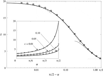
In figure 7 we test the uniformly valid approximation (6.5) for
 $\unicode[STIX]{x1D716}=0.01$
, along with approximations (6.2) and (6.3) for
 $\unicode[STIX]{x1D6FC}$
close to
 $\unicode[STIX]{x03C0}/2$
. We see that there is very good agreement throughout the entire range of protrusion angles
 $0\leqslant \unicode[STIX]{x1D6FC}\leqslant \unicode[STIX]{x03C0}/2$
. In the inset we demonstrate the efficacy of the uniform approximation also at larger
 $\unicode[STIX]{x1D716}$
values.
The normalised slip length
 $\unicode[STIX]{x1D706}$
as a function of protrusion angle
 $\unicode[STIX]{x1D6FC}$
for
 $\unicode[STIX]{x1D716}=0.01$
. The numerical data symbols (see text) are compared with the uniformly valid approximation (6.5) depicted by the thick solid line. Also shown, dash-dotted line: asymptotic expansion (6.2) for
 $\unicode[STIX]{x03C0}/2-\unicode[STIX]{x1D6FC}=O(\unicode[STIX]{x1D716}^{1/2})$
; dashed line: asymptotic expansion (6.3) for
 $\unicode[STIX]{x03C0}/2-\unicode[STIX]{x1D6FC}=O(\unicode[STIX]{x1D716})$
; thin line: asymptotic expansion (6.1) for
 $\unicode[STIX]{x03C0}/2-\unicode[STIX]{x1D6FC}=O(1)$
; upper dotted line: asymptotic expansion (1.3) for
 $\unicode[STIX]{x1D6FC}=\unicode[STIX]{x03C0}/2$
; lower dotted line: Philip’s solution (1.2) for
 $\unicode[STIX]{x1D6FC}=0$
. The inset demonstrates the agreement of the uniform approximation (6.5) with the numerical data also at larger values of
 $\unicode[STIX]{x1D716}$
.

6.4 Concluding remarks
The longitudinal slip length of a grooved surface is singular in the limit of vanishing solid fraction
 $\unicode[STIX]{x1D716}\rightarrow 0$
. For a flat meniscus, or more generally for protrusion angles not too close to
 $\unicode[STIX]{x03C0}/2$
, the singularity is very weak (logarithmic). Thus, for realistically small
 $\unicode[STIX]{x1D716}$
, the slip length is practically speaking commensurate with the period of the microstructure. On the other hand, for protrusion angles
 $\unicode[STIX]{x03C0}/2-\unicode[STIX]{x1D6FC}=O(\unicode[STIX]{x1D716}^{1/2})$
the singularity is algebraically strong, the slip length being
 $O(1/\unicode[STIX]{x1D716}^{1/2})$
large relative to the period. In this paper we have elucidated the origin of these different scalings and the transition between them by both scaling arguments and detailed asymptotics.
Several extensions to this work are desirable. First, the small-solid-fraction limit in the case of flow perpendicular to the bubbles remains an open problem (excluding the case of a flat interface). We do not expect in that case a transition to an algebraic small-solid-fraction singularity for protrusion angles close to
 $\unicode[STIX]{x03C0}/2$
, hence the prediction of large longitudinal slip lengths in that regime suggests strong anisotropy of the slip-length tensor
 $\unicode[STIX]{x1D740}$
. Second, a comparable analysis for the doubly periodic posts configuration would determine whether an asymptotic slip-length enhancement with increasing protrusion angles occurs as in the present case of a bubble mattress. This is particularly intriguing since for the posts configuration the slip length has an inverse-square-root singularity in the case of flat menisci. Third, it would be interesting to investigate what mechanisms are relevant in cutting off the slip-length singularity and at what orders of
 $\unicode[STIX]{x1D716}$
does a cutoff occur. One obvious mechanism is the internal circulation within the trapped bubbles (Schönecker, Baier & Hardt Reference Schönecker, Baier and Hardt2014), where even a small viscosity ratio will eventually (for small enough
 $\unicode[STIX]{x1D716}$
) enable an appreciable shear stress at the interface.
Lastly there is the connection between the effective slip length calculated for a semi-infinite liquid domain and the problem of flow – forced for example by a pressure gradient – through a finite channel with grooved boundaries (Sbragaglia & Prosperetti Reference Sbragaglia and Prosperetti2007). If the slip length is comparable to the surface periodicity while the macroscopic flow varies on a much larger scale (e.g. channel width) then the canonical semi-infinite slip problem appropriately describes the flow in the vicinity of the structured surface. However, in the small-solid-fraction limit – particularly for a doubly periodic array of posts and for a bubble mattress with
 $\unicode[STIX]{x1D6FC}\approx \unicode[STIX]{x03C0}/2$
– we have seen that the slip length inferred from the semi-infinite problem can be substantially larger than the period of the microstructure. The scale characterising the macroscale flow may therefore be large compared with the period but comparable to the slip length. There remains a separation of scales but the relation between the microhydrodynamics on the scale of the periodicity and the macroscopic flow is likely to be more involved. It is therefore not evident in that case that the macroscale boundary can be represented by an intrinsic effective-slip condition.
Acknowledgements
I am grateful to E. Luca and J. Marshall for sending me their code for calculating the slip length based on a ‘unified-transform’ method, which was used to produce the symbols in figures 6 and 7. I would also like to acknowledge useful discussions with E. Yariv, S. Hardt, and D. Crowdy.
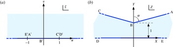
Conformal mapping used in appendix A.

Appendix A. Outer problem for
$0\leqslant \unicode[STIX]{x1D6FC}<\unicode[STIX]{x03C0}/2$

A.1 Formulation
We here solve the outer problem discussed in § 4. The field
 $g=w_{0}-\unicode[STIX]{x1D706}_{0}$
satisfies Laplace’s equation
 $$\begin{eqnarray}\unicode[STIX]{x1D6FB}^{2}g=0\end{eqnarray}$$
in the degenerate curvilinear triangle domain shown in figure 8(b), the far-field condition
 $$\begin{eqnarray}g\sim x+o(1)\quad \text{as }x\rightarrow \infty ,\end{eqnarray}$$
Neumann boundary conditions on all boundaries, and possesses the asymptotic behaviours
 $$\begin{eqnarray}g\sim \frac{1}{\unicode[STIX]{x03C0}/2-\unicode[STIX]{x1D6FC}}\ln \sqrt{x^{2}+(y\mp 1)^{2}}\quad \text{as }(x,y)=(0,\pm 1).\end{eqnarray}$$
Our interest is in the limit
 $$\begin{eqnarray}\mathscr{B}_{o}=\lim _{(x,y)\rightarrow (0,\pm 1)}\left(\frac{1}{\unicode[STIX]{x03C0}/2-\unicode[STIX]{x1D6FC}}\ln \sqrt{x^{2}+(y\mp 1)^{2}}-g\right),\end{eqnarray}$$
which is minus the constant correction term in (A 3).
A.2 Conformal mapping
The above problem is solved with the help of a conformal mapping. Specifically, we define complex variables
 $z=x+\text{i}y$
and
 $\unicode[STIX]{x1D701}=u+\text{i}v$
and show that
 $$\begin{eqnarray}z=\text{i}-2\cot \unicode[STIX]{x1D6FC}+\frac{2\sqrt{\unicode[STIX]{x03C0}}\csc \unicode[STIX]{x1D6FC}}{\unicode[STIX]{x1D6E4}(1/2+\unicode[STIX]{x1D6FC}/\unicode[STIX]{x03C0})\unicode[STIX]{x1D6E4}(1-\unicode[STIX]{x1D6FC}/\unicode[STIX]{x03C0})}\frac{F(1/2,\unicode[STIX]{x1D6FC}/\unicode[STIX]{x03C0},1/2+\unicode[STIX]{x1D6FC}/\unicode[STIX]{x03C0},\unicode[STIX]{x1D701})}{F(1/2,\unicode[STIX]{x1D6FC}/\unicode[STIX]{x03C0},1,1-\unicode[STIX]{x1D701})}\end{eqnarray}$$
maps the ‘auxiliary’ lower half-plane
 $v<0$
to the physical domain embedded in the ‘physical’
 $z$
plane, with the vertices along the real axis of the auxiliary plane as shown in figure 8. In (A 5),
 $F$
is the hypergeometric function defined as
 $$\begin{eqnarray}F(a,b,c;\unicode[STIX]{x1D701})=\frac{\unicode[STIX]{x1D6E4}(c)}{\unicode[STIX]{x1D6E4}(b)\unicode[STIX]{x1D6E4}(c-b)}\int _{0}^{1}t^{b-1}(1-t)^{c-b-1}(1-\unicode[STIX]{x1D701}t)^{-a}\,\text{d}t,\end{eqnarray}$$
where
 $s^{p}=\exp (p\log s)$
, the argument of
 $s$
satisfying
 $-\unicode[STIX]{x03C0}<\text{arg}(s)<\unicode[STIX]{x03C0}$
. The hypergeometric function as defined above is single valued and analytic in the
 $\unicode[STIX]{x1D701}$
plane excluding the branch cut
 $\unicode[STIX]{x1D701}=u\geqslant 1$
along the real axis (Abramowitz & Stegun Reference Abramowitz and Stegun1972). The general theory of mapping to curvilinear triangles is discussed by Nehari (Reference Nehari1975) and Ablowitz & Fokas (Reference Ablowitz and Fokas2003). The mapping (A 5) is identical, up to a dilation and a rotation, to the one given by Morris (Reference Morris2003). That author, however, appears to ignore the discontinuity of
 $F$
along the branch cut and deduces that the mapping to the physical domain is from the upper rather than the lower half of the auxiliary plane. In what follows we verify in detail the correctness of (A 5).
Let us first review certain properties of the hypergeometric function. The discontinuity along the branch cut can be made explicit by considering
 $\unicode[STIX]{x1D701}=1+\unicode[STIX]{x1D709}+\text{i}\unicode[STIX]{x1D6FF}$
(
 $\unicode[STIX]{x1D709}$
real and positive,
 $\unicode[STIX]{x1D6FF}$
real) in the limit where
 $\unicode[STIX]{x1D6FF}\rightarrow 0$
. Following Morris (Reference Morris2003), we split the integral in (A 6) into two parts:
 $$\begin{eqnarray}\displaystyle \!\!\lim _{\unicode[STIX]{x1D6FF}\rightarrow 0}F(a,b,c;1+\unicode[STIX]{x1D709}+\text{i}\unicode[STIX]{x1D6FF})\! & = & \displaystyle \!\frac{\unicode[STIX]{x1D6E4}(c)}{\unicode[STIX]{x1D6E4}(b)\unicode[STIX]{x1D6E4}(c-b)}\!\left[\int _{0}^{1/(1+\unicode[STIX]{x1D709})}\!t^{b-1}(1-t)^{c-b-1}[1-(1+\unicode[STIX]{x1D709})t]^{-a}\,\text{d}t\right.\nonumber\\ \displaystyle & & \displaystyle \!+\left.\lim _{\unicode[STIX]{x1D6FF}\rightarrow 0}\int _{1/(1+\unicode[STIX]{x1D709})}^{1}\!t^{b-1}(1-t)^{c-b-1}[1-(1+\unicode[STIX]{x1D709}+\text{i}\unicode[STIX]{x1D6FF})t]^{-a}\,\text{d}t\right]\!\!.\end{eqnarray}$$
The first integral in (A 7) is real and by a change of variables shown to be
 $$\begin{eqnarray}(1+\unicode[STIX]{x1D709})^{-b}\frac{\unicode[STIX]{x1D6E4}(b)\unicode[STIX]{x1D6E4}(1-a)}{\unicode[STIX]{x1D6E4}(1+b-a)}F\left(1+b-c,b,1+b-a,\frac{1}{1+\unicode[STIX]{x1D709}}\right)\!.\end{eqnarray}$$
The limit of the second integral in (A 7) depends on the sign of
 $\unicode[STIX]{x1D6FF}$
(this appears to have been overlooked by Morris (Reference Morris2003)). Making the change of variables
 $\unicode[STIX]{x1D706}\unicode[STIX]{x1D70F}=(1+\unicode[STIX]{x1D706})t-1$
we find
 $$\begin{eqnarray}\lim _{\unicode[STIX]{x1D6FF}\rightarrow 0}\frac{\unicode[STIX]{x1D709}^{c-b-a}}{(1+\unicode[STIX]{x1D709})^{c-1}}\int _{0}^{1}(1+\unicode[STIX]{x1D709}\unicode[STIX]{x1D70F})^{b-1}(1-\unicode[STIX]{x1D70F})^{c-b-1}\left(-\unicode[STIX]{x1D70F}-\text{i}\tilde{\unicode[STIX]{x1D6FF}}\right)^{-a}\,\text{d}\unicode[STIX]{x1D70F},\quad \tilde{\unicode[STIX]{x1D6FF}}=\unicode[STIX]{x1D6FF}\frac{1+\unicode[STIX]{x1D709}\unicode[STIX]{x1D70F}}{\unicode[STIX]{x1D709}(1+\unicode[STIX]{x1D709})},\end{eqnarray}$$
where
 $\tilde{\unicode[STIX]{x1D6FF}}$
and
 $\unicode[STIX]{x1D6FF}$
have the same sign and are of comparable magnitude. Noting that
 $$\begin{eqnarray}\displaystyle \lim _{\unicode[STIX]{x1D6FF}\rightarrow 0}(-\unicode[STIX]{x1D70F}-\text{i}\tilde{\unicode[STIX]{x1D6FF}})^{-a} & = & \displaystyle \lim _{\unicode[STIX]{x1D6FF}\rightarrow 0}\exp \left[-a\ln |\unicode[STIX]{x1D70F}+\text{i}\tilde{\unicode[STIX]{x1D6FF}}|-a\text{i}\,\text{arg}(-\unicode[STIX]{x1D70F}-\text{i}\tilde{\unicode[STIX]{x1D6FF}})\right]\nonumber\\ \displaystyle & = & \displaystyle \unicode[STIX]{x1D70F}^{-a}\text{e}^{\pm \text{i}\unicode[STIX]{x03C0}a}\quad \text{for }\unicode[STIX]{x1D6FF}\gtrless 0\end{eqnarray}$$
and substituting (A 8) and (A 9) into (A 7) yields the following formula for the jump across the branch cut:
 $$\begin{eqnarray}\displaystyle & & \displaystyle \lim _{\unicode[STIX]{x1D6FF}\rightarrow 0}F(a,b,c;1+\unicode[STIX]{x1D709}+\text{i}\unicode[STIX]{x1D6FF})\nonumber\\ \displaystyle & & \displaystyle ~=(1+\unicode[STIX]{x1D709})^{-b}\frac{\unicode[STIX]{x1D6E4}(c)\unicode[STIX]{x1D6E4}(1-a)}{\unicode[STIX]{x1D6E4}(c-b)\unicode[STIX]{x1D6E4}(1+b-a)}F\left(1+b-c,b,1+b-a,\frac{1}{1+\unicode[STIX]{x1D709}}\right)\nonumber\\ \displaystyle & & \displaystyle \quad ~+\,\frac{\text{e}^{\pm \text{i}\unicode[STIX]{x03C0}a}\unicode[STIX]{x1D709}^{c-b-a}}{(1+\unicode[STIX]{x1D709})^{c-1}}\frac{\unicode[STIX]{x1D6E4}(1-a)\unicode[STIX]{x1D6E4}(c)}{\unicode[STIX]{x1D6E4}(b)\unicode[STIX]{x1D6E4}(1+c-a-b)}F(1-b,1-a,1+c-a-b,-\unicode[STIX]{x1D709})\quad \text{for }\unicode[STIX]{x1D6FF}\gtrless 0.\nonumber\\ \displaystyle & & \displaystyle\end{eqnarray}$$
Note that the
 $F$
functions on the right-hand side of (A 11) are real and single valued.
We shall also require the asymptotic behaviour of the mapping (A 5) near the singular vertices
 $\unicode[STIX]{x1D701}=0$
and
 $\unicode[STIX]{x1D701}=1$
. From definition (A 6) it readily follows that
 $$\begin{eqnarray}\displaystyle & \displaystyle F(1/2,\unicode[STIX]{x1D6FC}/\unicode[STIX]{x03C0},1/2+\unicode[STIX]{x1D6FC}/\unicode[STIX]{x03C0},\unicode[STIX]{x1D701})\sim 1\quad \text{as }\unicode[STIX]{x1D701}\rightarrow 0, & \displaystyle\end{eqnarray}$$
 $$\begin{eqnarray}\displaystyle & \displaystyle F(1/2,\unicode[STIX]{x1D6FC}/\unicode[STIX]{x03C0},1,1-\unicode[STIX]{x1D701})\sim 1\quad \text{as }\unicode[STIX]{x1D701}\rightarrow 1, & \displaystyle\end{eqnarray}$$
while from relation (15.3.6) of Abramowitz & Stegun (Reference Abramowitz and Stegun1972) we deduce the asymptotic expansion
 $$\begin{eqnarray}\displaystyle \displaystyle F(1/2,\unicode[STIX]{x1D6FC}/\unicode[STIX]{x03C0},1,1-\unicode[STIX]{x1D701}) & {\sim} & \displaystyle \frac{\sqrt{\unicode[STIX]{x03C0}}\sec \unicode[STIX]{x1D6FC}}{\unicode[STIX]{x1D6E4}(1-\unicode[STIX]{x1D6FC}/\unicode[STIX]{x03C0})\unicode[STIX]{x1D6E4}(1/2+\unicode[STIX]{x1D6FC}/\unicode[STIX]{x03C0})}\nonumber\\ \displaystyle & & \displaystyle -\,\frac{\unicode[STIX]{x1D701}^{1/2-\unicode[STIX]{x1D6FC}/\unicode[STIX]{x03C0}}\sqrt{\unicode[STIX]{x03C0}}\sec \unicode[STIX]{x1D6FC}}{\unicode[STIX]{x1D6E4}(\unicode[STIX]{x1D6FC}/\unicode[STIX]{x03C0})\unicode[STIX]{x1D6E4}(3/2-\unicode[STIX]{x1D6FC}/\unicode[STIX]{x03C0})}\quad \text{as }\unicode[STIX]{x1D701}\rightarrow 0,\end{eqnarray}$$
which is valid for
 $-\unicode[STIX]{x03C0}<\arg (1-\unicode[STIX]{x1D701})<\unicode[STIX]{x03C0}$
. Consider now the singular limit of
 $F(1/2,\unicode[STIX]{x1D6FC}/\unicode[STIX]{x03C0},1/2+\unicode[STIX]{x1D6FC}/\unicode[STIX]{x03C0},\unicode[STIX]{x1D701})$
as
 $\unicode[STIX]{x1D701}\rightarrow 1$
. We write
 $\unicode[STIX]{x1D701}=1-r\exp (\text{i}\unicode[STIX]{x1D719})$
, where
 $r$
is real and
 $-\unicode[STIX]{x03C0}<\unicode[STIX]{x1D719}<\unicode[STIX]{x03C0}$
, and split the integral in (A 6) as
 $$\begin{eqnarray}F(1/2,\unicode[STIX]{x1D6FC}/\unicode[STIX]{x03C0},1/2+\unicode[STIX]{x1D6FC}/\unicode[STIX]{x03C0},\unicode[STIX]{x1D701})=\frac{\unicode[STIX]{x1D6E4}(\unicode[STIX]{x1D6FC}/\unicode[STIX]{x03C0}+1/2)}{\sqrt{\unicode[STIX]{x03C0}}\,\unicode[STIX]{x1D6E4}(\unicode[STIX]{x1D6FC}/\unicode[STIX]{x03C0})}\left({\mathcal{I}}_{1}+{\mathcal{I}}_{2}\right),\end{eqnarray}$$
where
 ${\mathcal{I}}_{1}$
and
 ${\mathcal{I}}_{2}$
are the integral
 $$\begin{eqnarray}\int t^{\unicode[STIX]{x1D6FC}/\unicode[STIX]{x03C0}-1}(1-t)^{-1/2}(1-t+rt\text{e}^{\text{i}\unicode[STIX]{x1D719}})^{-1/2}\,\text{d}t\end{eqnarray}$$
over the intervals
 $[0,1-\unicode[STIX]{x1D6FD}]$
and
 $[1-\unicode[STIX]{x1D6FD},1]$
, respectively; the arbitrary parameter
 $\unicode[STIX]{x1D6FD}$
is real, positive and satisfies
 $r\ll \unicode[STIX]{x1D6FD}\ll 1$
. In the first interval we can neglect the
 $r$
-dependent term, which yields
 $$\begin{eqnarray}{\mathcal{I}}_{1}\sim \int _{0}^{1-\unicode[STIX]{x1D6FD}}t^{\unicode[STIX]{x1D6FC}/\unicode[STIX]{x03C0}-1}(1-t)^{-1}\,\text{d}t\sim -\ln \unicode[STIX]{x1D6FD}-\unicode[STIX]{x1D6FE}_{E}-\unicode[STIX]{x1D713}(\unicode[STIX]{x1D6FC}/\unicode[STIX]{x03C0}).\end{eqnarray}$$
In the second interval
 $1-t\ll 1$
and following a change of variables we find
 $$\begin{eqnarray}{\mathcal{I}}_{2}\sim \int _{0}^{\unicode[STIX]{x1D6FD}/r}v^{-1/2}[v+\exp (\text{i}\unicode[STIX]{x1D719})]^{-1/2}\,\text{d}v\sim -\ln r+\ln \unicode[STIX]{x1D6FD}+\ln 4-\text{i}\unicode[STIX]{x1D719},\end{eqnarray}$$
where in the last step we evaluated the quadrature and expanded it for large
 $\unicode[STIX]{x1D6FD}/r$
. As it must be, the arbitrary parameter
 $\unicode[STIX]{x1D6FD}$
is seen to cancel out when adding together (A 17) and (A 18). Substituting these expansions into (A 15) we find
 $$\begin{eqnarray}\displaystyle & & \displaystyle \displaystyle F(1/2,\unicode[STIX]{x1D6FC}/\unicode[STIX]{x03C0},1/2+\unicode[STIX]{x1D6FC}/\unicode[STIX]{x03C0},\unicode[STIX]{x1D701})\nonumber\\ \displaystyle & & \displaystyle \quad \displaystyle \sim -\frac{\unicode[STIX]{x1D6E4}(1/2+\unicode[STIX]{x1D6FC}/\unicode[STIX]{x03C0})}{\sqrt{\unicode[STIX]{x03C0}}\,\unicode[STIX]{x1D6E4}(\unicode[STIX]{x1D6FC}/\unicode[STIX]{x03C0})}\left[\log (1-\unicode[STIX]{x1D701})-\ln 4+\unicode[STIX]{x1D6FE}_{E}+\unicode[STIX]{x1D713}(\unicode[STIX]{x1D6FC}/\unicode[STIX]{x03C0})\right]\quad \text{as }\unicode[STIX]{x1D701}\rightarrow 1,\quad\end{eqnarray}$$
which is valid for
 $-\unicode[STIX]{x03C0}<\arg (1-\unicode[STIX]{x1D701})<\unicode[STIX]{x03C0}$
. From the above asymptotic expansions we find that
 $$\begin{eqnarray}\displaystyle & \displaystyle z\sim -\frac{2}{\unicode[STIX]{x03C0}}\log (1-\unicode[STIX]{x1D701})+\text{i}-2\cot \unicode[STIX]{x1D6FC}+\frac{2}{\unicode[STIX]{x03C0}}\left[\ln 4-\unicode[STIX]{x1D6FE}_{E}-\unicode[STIX]{x1D713}(\unicode[STIX]{x1D6FC}/\unicode[STIX]{x03C0})\right]\quad \text{as }\unicode[STIX]{x1D701}\rightarrow 1, & \displaystyle\end{eqnarray}$$
 $$\begin{eqnarray}\displaystyle & \displaystyle z\sim \text{i}+2\cot \unicode[STIX]{x1D6FC}\frac{\unicode[STIX]{x1D6E4}(1/2+\unicode[STIX]{x1D6FC}/\unicode[STIX]{x03C0})\unicode[STIX]{x1D6E4}(1-\unicode[STIX]{x1D6FC}/\unicode[STIX]{x03C0})}{\unicode[STIX]{x1D6E4}(\unicode[STIX]{x1D6FC}/\unicode[STIX]{x03C0})\unicode[STIX]{x1D6E4}(3/2-\unicode[STIX]{x1D6FC}/\unicode[STIX]{x03C0})}\unicode[STIX]{x1D701}^{1/2-\unicode[STIX]{x1D6FC}/\unicode[STIX]{x03C0}}\quad \text{as }\unicode[STIX]{x1D701}\rightarrow 0. & \displaystyle\end{eqnarray}$$
We shall now verify that the real axis of the auxiliary plane, when approached from the lower half-plane, indeed maps onto the physical boundary. Consider first the interval
 $\text{A}^{\prime }\text{B}^{\prime }$
, on which both of the hypergeometric functions in (A 5) are real and continuous. It immediately follows that
 $\operatorname{Im}[z]=1$
; checking the end points using the asymptotic expansions (A 12), (A 13), (A 14) and (A 19) confirms that the range of
 $\operatorname{Re}\left(z\right)$
is
 $[\!0,\infty )$
. Hence
 $\text{A}^{\prime }\text{B}^{\prime }$
is mapped to AB.
Consider next the interval
 $\text{C}^{\prime }\text{D}^{\prime }$
, on which the hypergeometric function in the numerator of (A 5) is discontinuous. Its value when approached from the lower half-plane is found using (A 11):
 $$\begin{eqnarray}\displaystyle & & \displaystyle \text{C}^{\prime }\text{D}^{\prime }:\quad F\left(\frac{1}{2},\frac{\unicode[STIX]{x1D6FC}}{\unicode[STIX]{x03C0}},\frac{1}{2}+\frac{\unicode[STIX]{x1D6FC}}{\unicode[STIX]{x03C0}},\unicode[STIX]{x1D701}\right)\nonumber\\ \displaystyle & & \displaystyle \quad =(1+\unicode[STIX]{x1D709})^{-\unicode[STIX]{x1D6FC}/\unicode[STIX]{x03C0}}F\left(\frac{1}{2},\frac{\unicode[STIX]{x1D6FC}}{\unicode[STIX]{x03C0}},\frac{1}{2}+\frac{\unicode[STIX]{x1D6FC}}{\unicode[STIX]{x03C0}},\frac{1}{1+\unicode[STIX]{x1D709}}\right)\nonumber\\ \displaystyle & & \displaystyle \qquad \displaystyle -\,\text{i}(1+\unicode[STIX]{x1D709})^{1/2-\unicode[STIX]{x1D6FC}/\unicode[STIX]{x03C0}}\displaystyle \frac{\unicode[STIX]{x1D6E4}\left({\displaystyle \frac{1}{2}}+{\displaystyle \frac{\unicode[STIX]{x1D6FC}}{\unicode[STIX]{x03C0}}}\right)\unicode[STIX]{x1D6E4}\left({\displaystyle \frac{1}{2}}\right)}{\unicode[STIX]{x1D6E4}\left({\displaystyle \frac{\unicode[STIX]{x1D6FC}}{\unicode[STIX]{x03C0}}}\right)}F\left(1-\displaystyle \frac{\unicode[STIX]{x1D6FC}}{\unicode[STIX]{x03C0}},\frac{1}{2},1,-\unicode[STIX]{x1D709}\right),\end{eqnarray}$$
where
 $\unicode[STIX]{x1D701}=1+\unicode[STIX]{x1D709}>1$
. On the other hand, the hypergeometric function in the denominator of (A 5) is continuous. The mapping (A 5) accordingly yields
 $$\begin{eqnarray}\text{C}^{\prime }\text{D}^{\prime }:\quad \operatorname{Im}(z)=1-\frac{2\unicode[STIX]{x03C0}\csc \unicode[STIX]{x1D6FC}(1+\unicode[STIX]{x1D709})^{1/2-\unicode[STIX]{x1D6FC}/\unicode[STIX]{x03C0}}}{\unicode[STIX]{x1D6E4}(1-\unicode[STIX]{x1D6FC}/\unicode[STIX]{x03C0})\unicode[STIX]{x1D6E4}(\unicode[STIX]{x1D6FC}/\unicode[STIX]{x03C0})}\frac{F(1-\unicode[STIX]{x1D6FC}/\unicode[STIX]{x03C0},1/2,1,-\unicode[STIX]{x1D709})}{F(1/2,\unicode[STIX]{x1D6FC}/\unicode[STIX]{x03C0},1,-\unicode[STIX]{x1D709})};\end{eqnarray}$$
using relation (15.3.3) in Abramowitz & Stegun (Reference Abramowitz and Stegun1972) and the Euler reflection formula
 $\unicode[STIX]{x1D6E4}(z)\unicode[STIX]{x1D6E4}(1-z)=\unicode[STIX]{x03C0}\csc (\unicode[STIX]{x03C0}z)$
this reduces to
 $$\begin{eqnarray}\text{C}^{\prime }\text{D}^{\prime }:\quad \operatorname{Im}(z)=-1.\end{eqnarray}$$
The range of
 $\operatorname{Re}(z)$
can again be confirmed using the asymptotic expansions of the hypergeometric functions and hence
 $\text{C}^{\prime }\text{D}^{\prime }$
is mapped to CD.
It remains to verify that the interval
 $\text{B}^{\prime }\text{C}^{\prime \prime }$
is mapped to the circular segment BC. We write
 $\unicode[STIX]{x1D701}=-\unicode[STIX]{x1D709}+\text{i}\unicode[STIX]{x1D6FF}$
where
 $\unicode[STIX]{x1D709}$
is real and positive and
 $\unicode[STIX]{x1D6FF}$
is negative and arbitrarily small. This time the hypergeometric function in the numerator of (A 5) is continuous, whereas for the one in the denominator we use the jump relation (A 11):
 $$\begin{eqnarray}\displaystyle & & \displaystyle \displaystyle \text{B}^{\prime }\text{C}^{\prime \prime }:\quad F(1/2,\unicode[STIX]{x1D6FC}/\unicode[STIX]{x03C0},1,1-\unicode[STIX]{x1D701})\nonumber\\ \displaystyle & & \displaystyle \quad =\displaystyle \frac{(1+\unicode[STIX]{x1D709})^{-\unicode[STIX]{x1D6FC}/\unicode[STIX]{x03C0}}\sqrt{\unicode[STIX]{x03C0}}}{\unicode[STIX]{x1D6E4}(1-\unicode[STIX]{x1D6FC}/\unicode[STIX]{x03C0})\unicode[STIX]{x1D6E4}(1/2+\unicode[STIX]{x1D6FC}/\unicode[STIX]{x03C0})}F(\unicode[STIX]{x1D6FC}/\unicode[STIX]{x03C0},\unicode[STIX]{x1D6FC}/\unicode[STIX]{x03C0},1/2+\unicode[STIX]{x1D6FC}/\unicode[STIX]{x03C0},1/(1+\unicode[STIX]{x1D709}))\nonumber\\ \displaystyle & & \displaystyle \qquad \displaystyle +\,\text{i}\frac{\unicode[STIX]{x1D709}^{1/2-\unicode[STIX]{x1D6FC}/\unicode[STIX]{x03C0}}\sqrt{\unicode[STIX]{x03C0}}}{\unicode[STIX]{x1D6E4}(\unicode[STIX]{x1D6FC}/\unicode[STIX]{x03C0})\unicode[STIX]{x1D6E4}(3/2-\unicode[STIX]{x1D6FC}/\unicode[STIX]{x03C0})}F(1-\unicode[STIX]{x1D6FC}/\unicode[STIX]{x03C0},1/2,3/2-\unicode[STIX]{x1D6FC}/\unicode[STIX]{x03C0},-\unicode[STIX]{x1D709}).\end{eqnarray}$$
By substituting (A 25) into (A 5) we see that
 $\operatorname{Re}(z)>0$
; furthermore, the condition that
 $\text{B}^{\prime }\text{C}^{\prime \prime }$
maps on to the circle (2.3) can be reduced to
 $$\begin{eqnarray}\frac{\sqrt{\unicode[STIX]{x03C0}}\csc \unicode[STIX]{x1D6FC}}{\unicode[STIX]{x1D6E4}(1/2+\unicode[STIX]{x1D6FC}/\unicode[STIX]{x03C0})\unicode[STIX]{x1D6E4}(1-\unicode[STIX]{x1D6FC}/\unicode[STIX]{x03C0})}F(1/2,\unicode[STIX]{x1D6FC}/\unicode[STIX]{x03C0},1/2+\unicode[STIX]{x1D6FC}/\unicode[STIX]{x03C0},-\unicode[STIX]{x1D709})=l_{r}\cot \unicode[STIX]{x1D6FC}+l_{i},\end{eqnarray}$$
where
 $l_{r}$
and
 $l_{i}$
are respectively the real and imaginary part of (A 25); the equality is verified using the Euler reflection formula, along with relations (15.1.1) and (15.3.9) in Abramowitz & Stegun (Reference Abramowitz and Stegun1972).
A.3 Solution of the boundary value problem
We look for a solution in the form
 $g=\operatorname{Re}(T)$
, where
 $T(\unicode[STIX]{x1D701})$
is an analytical function in the lower half of the auxiliary plane. We first note that in order to satisfy conditions (A 2) and (A 3)
 $T$
should possess the expansions
 $$\begin{eqnarray}\displaystyle & \displaystyle T\sim z+o(1)\quad \text{as }\unicode[STIX]{x1D701}\rightarrow 1, & \displaystyle\end{eqnarray}$$
 $$\begin{eqnarray}\displaystyle & \displaystyle T\sim \frac{1}{\unicode[STIX]{x03C0}/2-\unicode[STIX]{x1D6FC}}\log (z-\text{i})+O(1)\quad \text{as }\unicode[STIX]{x1D701}\rightarrow 0. & \displaystyle\end{eqnarray}$$
(In (A 27) we could have allowed for an imaginary
 $O(1)$
term but that would have no effect on
 $g$
.) The above expansions together with the leading-order terms in (A 21) and (A 20) specify the strength of the sources to be placed at the singular vertices
 $\unicode[STIX]{x1D701}=0$
and
 $\unicode[STIX]{x1D701}=1$
(in § 3 we determined these from an integral argument). The existence of such sources is consistent with the Neumann condition on the boundary, and the
 $O(1)$
balance of (A 27) can be enforced by adding an appropriate constant determined from the two-term expansion (A 20). We thereby obtain the solution
 $$\begin{eqnarray}T=\frac{1}{\unicode[STIX]{x03C0}}\log \unicode[STIX]{x1D701}-\frac{2}{\unicode[STIX]{x03C0}}\log (1-\unicode[STIX]{x1D701})-2\cot \unicode[STIX]{x1D6FC}+\frac{2}{\unicode[STIX]{x03C0}}\ln 4-\frac{2}{\unicode[STIX]{x03C0}}\unicode[STIX]{x1D6FE}_{E}-\frac{2}{\unicode[STIX]{x03C0}}\unicode[STIX]{x1D713}(\unicode[STIX]{x1D6FC}/\unicode[STIX]{x03C0})+\text{i}.\end{eqnarray}$$
We can now use the two-term expansion (A 21) to inspect this solution near
 $\unicode[STIX]{x1D701}=0$
:
 $$\begin{eqnarray}\displaystyle \displaystyle \operatorname{Re}(T) & {\sim} & \displaystyle \frac{1}{\unicode[STIX]{x03C0}/2-\unicode[STIX]{x1D6FC}}\ln |z-\text{i}|-\frac{1}{\unicode[STIX]{x03C0}/2-\unicode[STIX]{x1D6FC}}\ln \left[\frac{2\cot \unicode[STIX]{x1D6FC}\,\unicode[STIX]{x1D6E4}(1-\unicode[STIX]{x1D6FC}/\unicode[STIX]{x03C0})\unicode[STIX]{x1D6E4}(1/2+\unicode[STIX]{x1D6FC}/\unicode[STIX]{x03C0})}{\unicode[STIX]{x1D6E4}(\unicode[STIX]{x1D6FC}/\unicode[STIX]{x03C0})\unicode[STIX]{x1D6E4}(3/2-\unicode[STIX]{x1D6FC}/\unicode[STIX]{x03C0})}\right]\nonumber\\ \displaystyle & & \displaystyle -\,2\cot \unicode[STIX]{x1D6FC}+\frac{2}{\unicode[STIX]{x03C0}}\ln 4-\frac{2}{\unicode[STIX]{x03C0}}\unicode[STIX]{x1D6FE}_{E}-\frac{2}{\unicode[STIX]{x03C0}}\unicode[STIX]{x1D713}(\unicode[STIX]{x1D6FC}/\unicode[STIX]{x03C0})\quad \text{as }\unicode[STIX]{x1D701}\rightarrow 0.\qquad\end{eqnarray}$$
According to (A 4) the requisite function
 $\mathscr{B}_{o}(\unicode[STIX]{x1D6FC})$
is provided as minus the
 $O(1)$
part in (A 30), which yields the result (4.7) stated in the main text.
Conformal mapping used in appendix B.

Appendix B. Inner problem for
$0\leqslant \unicode[STIX]{x1D6FC}<\unicode[STIX]{x03C0}/2$

B.1 Formulation
We here solve the inner problem of § 4 governing the field
 $W_{0}(X,Y)$
, where
 $X$
and
 $Y$
are the inner coordinates (4.8). It is convenient to consider the problem in the mirrored inner geometry shown in figure 9(b), with
 $W_{0}(-X,Y)=-W_{0}(X,Y)$
(cf. (4.11)). Recall from § 4 that
 $W_{0}$
satisfies Laplace’s equation (4.10), Neumann conditions on the boundaries (4.12), along with the prescribed far-field behaviour (4.13), which we repeat here:
 $$\begin{eqnarray}W_{0}\sim \pm \frac{1}{\unicode[STIX]{x03C0}/2-\unicode[STIX]{x1D6FC}}\ln \sqrt{X^{2}+Y^{2}}\quad \text{as }X^{2}+Y^{2}\rightarrow \infty ,\quad X\gtrless 0.\end{eqnarray}$$
Thus
 $W_{0}$
can be thought as the potential of an ideal flow of prescribed flux through a converging–diverging slit channel, with the additive freedom of the potential removed by condition (4.11). The goal of the calculation is to extract the limit
 $$\begin{eqnarray}\mathscr{B}_{i}=\lim _{X^{2}+Y^{2}\rightarrow \infty }\left(\pm W_{0}-\frac{1}{\unicode[STIX]{x03C0}/2-\unicode[STIX]{x1D6FC}}\ln \sqrt{X^{2}+Y^{2}}\right),\quad X\gtrless 0,\end{eqnarray}$$
which can be interpreted as the blockage coefficient or excess resistance of the envisaged channel. As in appendix A, we first introduce a conformal mapping from an auxiliary half-space to the physical domain and then use the asymptotics of the mapping near the critical points to find the appropriate solution. Our derivation is similar to that of Yariv & Sherwood (Reference Yariv and Sherwood2015) for the excess resistance of a slot of finite thickness.
B.2 Conformal mapping
We introduce a mapping from the upper half of the auxiliary plane
 $\unicode[STIX]{x1D701}=u+\text{i}v$
to the physical domain in the plane
 $Z=X+\text{i}Y$
. Using the Schwarz–Christoffel formula (Ablowitz & Fokas Reference Ablowitz and Fokas2003) and fixing the singular points of the mapping as in figure figure 8, we find
 $$\begin{eqnarray}Z=M\int _{0}^{\unicode[STIX]{x1D701}}\frac{t^{1-2\unicode[STIX]{x1D6FC}/\unicode[STIX]{x03C0}}}{(t^{2}-1)^{3/2-\unicode[STIX]{x1D6FC}/\unicode[STIX]{x03C0}}}\,\text{d}t+\text{i},\end{eqnarray}$$
where
 $M$
is a constant to be determined by the requirement that
 $\unicode[STIX]{x1D701}=\text{i}\infty$
is mapped to
 $Z=0$
. In this appendix we choose the branch of the complex power as
 $t^{p}=|t|^{p}\exp (\text{i}p\unicode[STIX]{x1D70F})$
, where
 $\unicode[STIX]{x1D70F}=\arg (t)\in (-\unicode[STIX]{x03C0}/2,3\unicode[STIX]{x03C0}/2)$
. To determine
 $M$
, we set
 $Z=0$
, and make the change of variables in the integral
 $t=\text{i}\unicode[STIX]{x1D702}$
,
 $$\begin{eqnarray}1=M\int _{0}^{\infty }\frac{\unicode[STIX]{x1D702}^{1-2\unicode[STIX]{x1D6FC}/\unicode[STIX]{x03C0}}}{(1+\unicode[STIX]{x1D702}^{2})^{3/2-\unicode[STIX]{x1D6FC}/\unicode[STIX]{x03C0}}}\,\text{d}\unicode[STIX]{x1D702}.\end{eqnarray}$$
Evaluating the quadrature we find
 $$\begin{eqnarray}M=\frac{2\unicode[STIX]{x1D6E4}(3/2-\unicode[STIX]{x1D6FC}/\unicode[STIX]{x03C0})}{\sqrt{\unicode[STIX]{x03C0}}\,\unicode[STIX]{x1D6E4}(1-\unicode[STIX]{x1D6FC}/\unicode[STIX]{x03C0})}.\end{eqnarray}$$
In what follows we shall require the asymptotics of the mapping as
 $\unicode[STIX]{x1D701}\rightarrow \pm 1$
, which corresponds in the physical domain to the far-field limits
 $X^{2}+Y^{2}\rightarrow \infty$
 $(X\lessgtr 0)$
. In particular, following Yariv & Sherwood (Reference Yariv and Sherwood2015) and using integration by parts in (B 3) we find the asymptotic behaviour
 $$\begin{eqnarray}Z\sim -\frac{M}{2^{3/2-\unicode[STIX]{x1D6FC}/\unicode[STIX]{x03C0}}(1/2-\unicode[STIX]{x1D6FC}/\unicode[STIX]{x03C0})}\frac{1}{(\unicode[STIX]{x1D701}-1)^{1/2-\unicode[STIX]{x1D6FC}/\unicode[STIX]{x03C0}}}\quad \text{as }\unicode[STIX]{x1D701}\rightarrow 1.\end{eqnarray}$$
B.3 Solution of the boundary value problem
We look for a solution in the form
 $W_{0}=\operatorname{Re}(T)$
, where
 $T(\unicode[STIX]{x1D701})$
is an analytic function in the upper half of the auxiliary plane. To satisfy the far-field singularities (B 1) we place the appropriate potential sources at
 $\unicode[STIX]{x1D701}=\pm 1$
. The potential associated with these sources is consistent with the Neumann conditions on the boundary whereby we arrive at the solution
 $$\begin{eqnarray}T(\unicode[STIX]{x1D701})=\frac{1}{\unicode[STIX]{x03C0}}\log \frac{\unicode[STIX]{x1D701}-1}{\unicode[STIX]{x1D701}+1}.\end{eqnarray}$$
We can now use (B 6) to calculate the limit (B 2). Substituting expansion (B 6) into (B 7) we find
 $$\begin{eqnarray}\displaystyle -W_{0} & {\sim} & \displaystyle \frac{1}{\unicode[STIX]{x03C0}/2-\unicode[STIX]{x1D6FC}}\ln \sqrt{X^{2}+Y^{2}}\nonumber\\ \displaystyle & & \displaystyle +\,\frac{1}{\unicode[STIX]{x03C0}/2-\unicode[STIX]{x1D6FC}}\ln \frac{4^{1-\unicode[STIX]{x1D6FC}/\unicode[STIX]{x03C0}}(1/2-\unicode[STIX]{x1D6FC}/\unicode[STIX]{x03C0})}{M}+o(1)\quad \text{as }X^{2}+Y^{2}\rightarrow \infty ,\quad X<0.\qquad\end{eqnarray}$$
Substitution of (B 5) into (B 8) and applying (B 1) yields formula (4.15) for
 $\mathscr{B}_{i}(\unicode[STIX]{x1D6FC})$
.