

1 Introduction
Thin films of electrolyte solution have a widespread presence in various fields of science and engineering, such as wetting (Bénichou et al. Reference Bénichou, Cachile, Cazabat, Poulard, Valignat, Vandenbrouck and Van Effenterre2003), colloidal interaction (Russel, Saville & Schowalter Reference Russel, Saville and Schowalter1989), emulsion stability (Aronson & Princen Reference Aronson and Princen1980), bubble coalescence (Craig Reference Craig2004), mineral floatation (Albijanic et al. Reference Albijanic, Ozdemir, Nguyen and Bradshaw2010), lubrication (Chakraborty & Chakraborty Reference Chakraborty and Chakraborty2011), microfluidics and nanofluidics (Li Reference Li2008) etc. These films are formed by confining electrolyte solutions in between two charged surfaces, and their thickness, defined by the separation of the two confining surfaces, is usually of the order of micro/nanometres. Each charged surface electrostatically attracts counterions of electrolyte to the surface, and repel coions of electrolyte away from the surface to form a so-called electric double layer (EDL) near the corresponding surface. The thickness of the EDL is usually a few nanometres and decreases with increasing electrolyte concentration. The two charged surfaces interact with each other due to the finite overlap of the two EDLs on the surfaces. Such interaction due to the EDL overlap is quite crucial for understanding the properties of thin electrolyte solution films, such as stability, drainage and rupture (Tambe & Sharma Reference Tambe and Sharma1994; Valkovska & Danov Reference Valkovska and Danov2001; Manev & Nguyen Reference Manev and Nguyen2005; Craig Reference Craig2011).
Generally, there are two categories of interaction between two charged surfaces confining electrolyte solution films: (i) when the solution and charged surfaces are both stationary, the two surfaces interact purely electrostatically as the EDLs on the two surfaces overlap, and the resulting interaction force is conservative in nature; (ii) when there is a relative motion between the solution and the charged surfaces, apart from the conservative EDL force, the surfaces would experience a flow-induced hydrodynamic force, and such a force is dissipative in nature. The first category represents an ideal case which corresponds precisely to the electrostatic component of the well-known Derjaguin–Landau–Verwey–Overbeek (DLVO) force (i.e. EDL force), and the second category is more frequently encountered since, in practice, there is usually inevitable relative motion between the solution and charged surfaces, such as colloidal particles undergoing Brownian motion in the solution and colloidal particles subject to external flows in various applications. The theory of the first category is adequately described by the electrostatics of EDL alone, and the (conservative) interaction force in this category can be readily evaluated from the well-developed and widely accepted DLVO theory (Derjaguin et al. Reference Derjaguin, Churaev, Muller and Kitchener1987; van de Ven Reference van de Ven1989; Masliyah & Bhattacharjee Reference Masliyah and Bhattacharjee2006). For the theory of the second category, the current literature mostly takes the conservative EDL force from the DLVO theory for granted, and focuses on the calculation of the dissipative hydrodynamic force (Bike & Prieve Reference Bike and Prieve1990, Reference Bike and Prieve1995; Muller Reference Muller1990; Warszyski & van de Ven Reference Warszyski and van de Ven1991; Cox Reference Cox1997; Warszyski Reference Warszyski2000; Chun & Ladd Reference Chun and Ladd2004; Tabatabaei & van de Ven Reference Tabatabaei and van de Ven2010). These studies generally revealed that the hydrodynamic force is enhanced by the so-called electroviscous effect arising from a coupling between the electrostatics and hydrodynamics of EDL. Additionally, the study of the dissipative hydrodynamic interaction force in this category has two situations according to the manner in which the two surfaces move relative to each other, i.e. one surface squeezing vertically towards the other and one surface sliding parallelly over the other. The problem of one surface squeezing vertically towards the other was firstly analysed by Bike & Prieve (Reference Bike and Prieve1990) who calculated the hydrodynamic interaction force of two spherical particles as the electrolyte solution film is squeezed out of the gap between the two particles. In addition to the hydrodynamic interaction force that uncharged particles experience, an additional electroviscous interaction force was discovered. Their calculation was performed under the lubrication and thin EDL assumptions. Similarly, Muller (Reference Muller1990) also adopted the lubrication approximation to analyse the squeezing flow between two charged parallel disks and calculated the corresponding electroviscous interaction force, and the results of two parallel disks were further utilized to evaluate the electroviscous interaction force between two spheres using the Derjaguin approximation. Their results are applicable to thick EDL situations (overlapping EDLs), but they assumed an equal diffusivity for cations and anions. Warszyski & van de Ven (Reference Warszyski and van de Ven1990) also performed an analysis of the electroviscous interaction force between two parallel disks under the squeezing flow, and the results were transformed to sphere–wall and sphere–sphere interactions using the Derjaguin approximation. The same authors later discussed how the electroviscous effect modifies the squeezing flow field between the two parallel disks (Warszyski & van de Ven Reference Warszyski and van de Ven1991). However, their analyses were based on the unrealistic assumption that the electric current density is zero everywhere inside the solution films. The various assumptions made in the aforementioned studies, e.g. thin EDL and locally zero electric current density, have been shown to produce substantially erroneous or unphysical predictions of the electroviscous force under certain conditions by Chun & Ladd (Reference Chun and Ladd2004). The most recent work by Talapatra & Chakraborty (Reference Talapatra and Chakraborty2009) analysed the squeezing flow between two charged parallel plates with the electroviscous effect, whereas no information regarding the interaction force was revealed.
The electroviscous interaction force in the problem of one surface squeezing vertically towards the other has only one component, which is directed to the opposite moving direction of the surface. Nevertheless, in the problem of one surface sliding parallelly over the other, the electroviscous interaction force has two components (Bike & Prieve Reference Bike and Prieve1990; Warszyski & van de Ven Reference Warszyski and van de Ven2000): the first component is opposite to the moving direction of surface, and is called the electroviscous drag force; the second component is normal to the moving direction of the surface, and tends to push the two surfaces apart, and is dubbed the electrokinetic lift force in the literature. The study of the electroviscous drag force is quite limited, while the study of the electrokinetic lift force has been a focus since its discovery in 1980s (Alexander & Prieve Reference Alexander and Prieve1987), because this phenomenon is potentially related to a number of applications, such as colloidal particles adsorption (Warszyski Reference Warszyski2000), capillary hydrodynamic fractionation (Hollingsworth & Silebi Reference Hollingsworth and Silebi1996) and hydrodynamic chromatography (Striegel & Brewer Reference Striegel and Brewer2012), tribology (Bo & Umehara Reference Bo and Umehara1998) etc. The experimental studies systematically studied the effects of shear, medium conductivity, ionic strength and zeta ( $\unicode[STIX]{x1D701}$) potential on the electrokinetic lift force (Bike, Lazarro & Prieve Reference Bike, Lazarro and Prieve1995; Wu, Warszyski & van de Ven Reference Wu, Warszyski and van de Ven1996). The theory for the electrokinetic lift force has undergone two phases of development and improvement. Initially, the theory of the electrokinetic lift force was developed for an ionic Péclet number that is much less than unity (Bike & Prieve Reference Bike and Prieve1990, Reference Bike and Prieve1992, Reference Bike and Prieve1995; van de Ven, Warszyski & Dukhin Reference van de Ven, Warszyski and Dukhin1993). Bike & Prieve (Reference Bike and Prieve1990) derived the first analytical expression for the electrokinetic lift force between a spherical particle and a wall under the lubrication and thin EDL assumptions. The same authors later adopted the reflection method to calculate the electrokinetic lift force for a particle–wall separation much larger than the particle radius (Bike & Prieve Reference Bike and Prieve1992), and van de Ven et al. (Reference van de Ven, Warszyski and Dukhin1993) performed an analysis for a similar situation. Later on, Bike & Prieve (Reference Bike and Prieve1995) relaxed the lubrication approximation in their previous study to analyse the electrokinetic lift force for an arbitrary particle–wall separation. However, the electrokinetic lift force predicted from these theories is several orders of magnitude lower than the experimentally measured value, presumably due to the low ionic Péclet number assumption in these theories (see Wu et al. Reference Wu, Warszyski and van de Ven1996). Practically, the conditions in electrokinetic lift force experiments, including the shear flow/particle velocity, medium viscosity and electrolyte concentration, can easily result in an ionic Péclet number of the order of unity or higher, thereby invalidating the low ionic Péclet number assumption. The Warszyński group first recognized the effect of large ionic Péclet number and accordingly modified the electrokinetic lift theory to account for such an effect (Warszyski, Wu & van de Ven Reference Warszyski, Wu and van de Ven1998; Warszyski & van de Ven Reference Warszyski and van de Ven2000). They analysed the electrokinetic lift force on a charged cylinder sliding over a charged wall under the lubrication and thin EDL assumptions. Then, they used the Derjaguin approximation to transform the electrokinetic lift force of a cylinder–wall configuration to that of a sphere–wall configuration. To account for the effect of large ionic Péclet number, they expanded the analytical solutions of all relevant variables in a series of ionic Péclet number, and then retained the terms up to the second power of Péclet number in the analysis. In addition, three fundamental modes of the flow field were considered in their investigations: the cylinder/sphere translating over the wall with no rotation in a stagnant fluid, the cylinder/sphere rotating over the wall with no translation in a stagnant fluid and the stationary cylinder/sphere in the wall shear flow, since generally the electrokinetic lift force for a spherical particle moving near a wall can be obtained as a superposition of the three fundamental modes (Goldman, Cox & Brenner Reference Goldman, Cox and Brenner1967; Goren & O’Neill Reference Goren and O’Neill1971; Warszyski et al. Reference Warszyski, Wu and van de Ven1998). The electrokinetic lift force predicted with the theory of large ionic Péclet number has been shown to agree quite well with the experimental measurements (Bike et al. Reference Bike, Lazarro and Prieve1995; Wu et al. Reference Wu, Warszyski and van de Ven1996; Warszyski Reference Warszyski2000).
Notably, the previously discussed various electroviscous effects in the interaction of two charged surfaces have the same origin as the more widely known electroviscous effect in pressure-driven flows inside charged capillaries, which typically demonstrate a flow rate reduction or an increment of apparent liquid viscosity relative to the uncharged condition (Burgreen & Nakache Reference Burgreen and Nakache1964; Rice & Whitehead Reference Rice and Whitehead1965; Levine et al. Reference Levine, Marriott, Neale and Epstein1975; Ren & Li Reference Ren and Li2004; Li Reference Li2008). Essentially, all electroviscous effects produce extra resistance to the external flow due to the presence of EDLs. The convective transport of ionic charge in EDLs with the external flow induces a streaming current, and this current further leads to a separation of charge, which generates a streaming potential field parallel to the flow direction. The streaming potential field, in turn, drives a back electroosmotic flow to oppose the external flow, inducing either an electroviscous force in the interaction of two charged surfaces or a flow rate reduction in pressure-driven flows.
Reviewing the investigations of various types of electroviscous effect, we note that the theories of the electroviscous effect in pressure-driven flows and the electrokinetic lift force are well established since they have been firmly validated by experimental measurements (Wu et al. Reference Wu, Warszyski and van de Ven1996; Warszyski et al. Reference Warszyski, Wu and van de Ven1998; Warszyski & van de Ven Reference Warszyski and van de Ven2000; Li Reference Li2001; Ren & Li Reference Ren and Li2004) However, for the electroviscous effect in the case of one charged surface squeezing vertically towards another charged surface, both the experimental and theoretical studies are not satisfactory at the moment. For the experimental studies, previous investigations used the surface force apparatus (see Israelachvili Reference Israelachvili1986; Raviv, Laurat & Klein Reference Raviv, Laurat and Klein2001; Raviv et al. Reference Raviv, Perkin, Laurat and Klein2004) and the colloid probe atomic force microscope (AFM, see Craig, Neto & Williams (Reference Craig, Neto and Williams2001), Bonaccurso, Kappl & Butt (Reference Bonaccurso, Kappl and Butt2002), Vinogradova & Yakubov (Reference Vinogradova and Yakubov2003), Honig & Ducker (Reference Honig and Ducker2007) and Henry & Craig (Reference Henry and Craig2009)) to measure the dissipative hydrodynamic interaction force in the squeezing flows of thin electrolyte solution films, but unanimously did not detect the electroviscous effect, probably due to the low surface charge density or the increase of the fluid viscosity by sucrose in these experiments. Only recently, Liu et al. (Reference Liu, Klaassen, Zhao, Mugele and van den Ende2018) utilized the dynamic AFM with an oscillating tip to measure the dissipative hydrodynamic force as a thin film of aqueous NaCl solution was squeezed out of the gap between the tip and the substrate. The dynamic AFM is advantageous over other techniques since it prevents the snap-in stability for small tip–substrate separation. The experiment was done under well-controlled conditions. The tip and substrate were both oxidized silicon. The tip was spherical and the substrate flat, which mimicked the standard sphere–wall configuration. The concentration and pH of the NaCl solution were adjusted to control the surface charge on the tip and substrate. The authors clearly observed a surface-charge-induced enhancement of the dissipative hydrodynamic force during the interaction of the tip and the substrate. Nevertheless, the electroviscous origin of such dissipation enhancement is yet to be confirmed. For the theoretical studies, as mentioned previously, the current literature contains various assumptions, such as a thin EDL, equal ion diffusivity and zero local current density etc. Moreover, formulations of previous theoretical models are mostly based on the configuration of two parallel flat surfaces, and thus lack an apparent link to the more practical configuration with curved surfaces that is more frequently encountered in experiments.
It is clear from the above discussion that the dynamic AFM holds great potential for detecting the electroviscous effects in squeezing flows. In the present work, we present a detailed analysis of the electroviscous effects on the squeezing flow of a thin electrolyte solution film in a tip–substrate configuration abstracted from the dynamic AFM experiment. The analysis considering the dynamic effect (oscillatory motion of charged surfaces) is also potentially relevant to some other practical situations, such as Brownian collisions between colloid particles (Warszyski & van de Ven Reference Warszyski and van de Ven1991) and dynamic rheometry (Engmann, Servais & Burbidge Reference Engmann, Servais and Burbidge2005). Our analysis considering the coupling of hydrodynamics and electrostatics in EDLs shows that the interaction force between two surfaces as one squeezes toward the other can be self-consistently derived as a superposition of one conservative component and one dissipative component. The conservative component proves to be precisely the EDL force in the DLVO theory and the dissipative component is found to be the hydrodynamic force enhanced by the electroviscous effect. This is different from the current literature, which frequently treats the conservative EDL force and the dissipative hydrodynamic force independently. To understand the studied electroviscous effect more intuitively, we give a detailed discussion of how the electroviscous effect modifies the flow field inside the thin films. The study also introduces a power-law index to address the influence of surface profiles on the electroviscous effect quantitatively; this is relevant to the possibility of varying tip profiles in the dynamic AFM experiments.
The paper is organized as follows: § 2 reviews the general electrokinetic theory and governing equations which are to be used in the analysis; § 3 presents derivations of the interaction force (both conservative EDL force and dissipative hydrodynamic force) between two charged surfaces as a thin film of electrolyte solution is squeezed out of the gap between the two surfaces and the analytical solution of the electroviscous-effect-modified flow field inside the thin electrolyte film. In § 4, we mainly discuss the electroviscous-effect-modified flow field in the thin electrolyte films and the influence of various parameters (e.g. electrokinetic separation,  $\unicode[STIX]{x1D701}$ potential, surface profiles and electrolytes) on the electroviscous effect, and § 5 summarizes the main findings and points out the direction for improving the current model.
2 Electrokinetic theory
Electrokinetic theory deals with the transport of ions and liquids in electric fields (Probstein Reference Probstein1994; Masliyah & Bhattacharjee Reference Masliyah and Bhattacharjee2006). The theory was initially developed in the colloid science field to understand colloid interaction and stability, and nowadays is a useful tool to understand micro- and nano-scale transport phenomena in aqueous liquid environments. Generally, a full mathematical formulation of the electrokinetic theory consists of the governing equations for the ion and liquid transport, and the electric field distribution. The transport of ions is governed by the Nernst–Planck mass conservation equation
 $$\begin{eqnarray}\frac{\unicode[STIX]{x2202}N_{k}}{\unicode[STIX]{x2202}t}+\unicode[STIX]{x1D735}\boldsymbol{\cdot }\boldsymbol{J}_{k}=0,\end{eqnarray}$$
where  $t$ is the time and
 $$\begin{eqnarray}\boldsymbol{J}_{k}=n_{k}\boldsymbol{u}-D_{k}\unicode[STIX]{x1D735}N_{k}-\frac{Z_{k}eN_{k}D_{k}}{k_{B}T}\unicode[STIX]{x1D735}\unicode[STIX]{x1D713}\end{eqnarray}$$
is the ionic flux that is composed of the contributions from liquid convection ( $N_{k}\boldsymbol{u}$), diffusion (
 $-D_{k}\unicode[STIX]{x1D735}N_{k}$) and electrophoretic migration (
 $-Z_{k}eN_{k}D_{k}\unicode[STIX]{x1D735}\unicode[STIX]{x1D713}/(k_{B}T)$). Electric current density in the liquid can be evaluated as
 $\boldsymbol{i}=e\sum _{k}Z_{k}\boldsymbol{J}_{k}$. In (2.2),
 $\boldsymbol{u}$ denotes the liquid velocity vector,
 $\unicode[STIX]{x1D713}$ is electric potential,
 $e$ is the elementary charge,
 $k_{B}$ is the Boltzmann constant,
 $T$ is the absolute temperature,
 $N_{k}$,
 $Z_{k}$ and
 $D_{k}$ are the number concentration, the valence and the diffusion coefficient of ion species
 $k$, respectively.
Because of the presence of an ionic charge in liquids, the liquid frequently experiences an electrostatic body force which modifies the liquid (momentum) transport equation to be
 $$\begin{eqnarray}\unicode[STIX]{x1D70C}(\unicode[STIX]{x2202}_{t}+\boldsymbol{u}\boldsymbol{\cdot }\unicode[STIX]{x1D735})\boldsymbol{u}=-\unicode[STIX]{x1D735}p+\unicode[STIX]{x1D707}\unicode[STIX]{x1D6FB}^{2}\boldsymbol{u}-\unicode[STIX]{x1D70C}_{e}\unicode[STIX]{x1D735}\unicode[STIX]{x1D713},\end{eqnarray}$$
where  $\unicode[STIX]{x1D70C}$ is the liquid density,
 $\unicode[STIX]{x1D707}$ is the liquid viscosity,
 $p$ is the pressure and the ionic charge density
 $\unicode[STIX]{x1D70C}_{e}$ is evaluated from the local ion concentration by
 $\unicode[STIX]{x1D70C}_{e}=e\sum _{k}N_{k}Z_{k}$. In addition to the momentum balance, the liquid transport is also subject to the mass conservation
 $$\begin{eqnarray}\unicode[STIX]{x1D735}\boldsymbol{\cdot }\boldsymbol{u}=0.\end{eqnarray}$$
It is noted that (2.3) and (2.4) require that the liquids are incompressible.
The electric potential, which contributes to both the ion and liquid transport, is governed by the Poisson equation
 $$\begin{eqnarray}\unicode[STIX]{x1D700}\unicode[STIX]{x1D6FB}^{2}\unicode[STIX]{x1D713}=-\unicode[STIX]{x1D70C}_{e},\end{eqnarray}$$
where  $\unicode[STIX]{x1D700}$ is the liquid dielectric permittivity.
To evaluate the force exerted on one surface immersed in the liquid, one can use the total stress which is due to the pressure, viscous stress and Maxwell stress, and can be expressed in the tensor form as
 $$\begin{eqnarray}\unicode[STIX]{x1D64F}=-p\unicode[STIX]{x1D644}+\unicode[STIX]{x1D707}[\unicode[STIX]{x1D735}\boldsymbol{u}+(\unicode[STIX]{x1D735}\boldsymbol{u})^{\text{T}}]+\unicode[STIX]{x1D700}\left(A\boldsymbol{A}-{\textstyle \frac{1}{2}}E^{2}\unicode[STIX]{x1D644}\right),\end{eqnarray}$$
where  $\unicode[STIX]{x1D644}$ is the second-order unit tensor,
 $\boldsymbol{E}=-\unicode[STIX]{x1D735}\unicode[STIX]{x1D713}$ the electric field and
 $E^{2}=\boldsymbol{E}\boldsymbol{\cdot }\boldsymbol{E}$. It should be mentioned here that there exist extra stresses acting on the surface due to the universally present van der Waals and short-range hydration forces etc. (Israelachvili Reference Israelachvili2011), which are not included in (2.6) and can be taken into consideration during the calculation of the total interaction force.
Equations (2.1)–(2.5) together with appropriate initial and boundary conditions present a general description of electrokinetic transport phenomena. Seemingly, these equations are highly coupled, the analytical solution of them could be very difficult or almost impossible. However, under some special situations, these equations can be solved analytically. One particular example is the no liquid flow situation, namely,  $\boldsymbol{u}=\mathbf{0}$. Firstly, the solution of (2.1) and (2.2) gives rise to the Boltzmann distribution of ions. Secondly, substituting the Boltzmann distribution of ions in (2.5), we can obtain the governing equation for the EDL potential, i.e. the Poisson–Boltzmann equation. Then, the EDL potential can be solved from this equation. Thirdly, with the solution of the EDL potential, one can obtain the solution of the static pressure (or osmotic pressure) from (2.3) and (2.4). Finally, one substitutes the osmotic pressure into (2.6) to obtain the EDL force (i.e. the electrostatic part of the DLVO force).
Another example is the more practical case with liquid flow (as is shown in § 3), with some reasonable assumptions (e.g. low Reynolds and ionic Péclet numbers), the liquid transport ((2.3) and (2.4)), ion transport ((2.1) and (2.2)) and electric potential (2.5) can be decoupled, and thus the problem can be solved analytically.
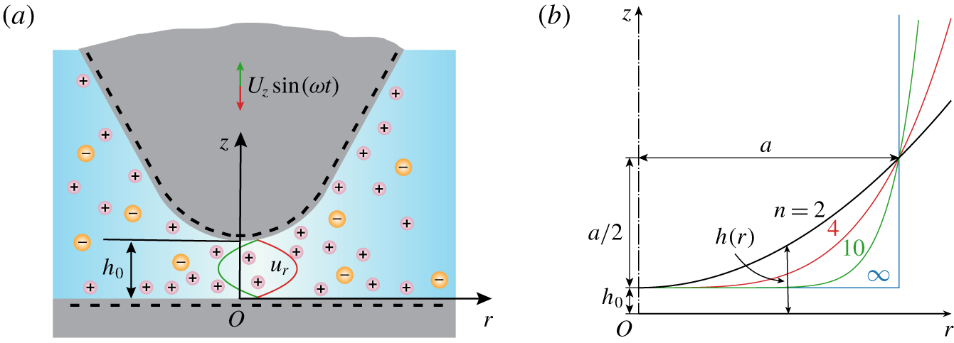
(a) Schematics of the model system in an axisymmetric cylindrical coordinate system ( $r$,
 $z$). The tip oscillates with a velocity of
 $U_{z}\sin (\unicode[STIX]{x1D714}t)$ above the substrate with a time-averaged separation of
 $h_{0}$, and the amplitude of oscillation is much smaller than
 $h_{0}$. Both the tip and substrate surfaces are negatively charged because of the presence of an aqueous electrolyte solution in the gap, and then the tip EDL and substrate EDL overlap to induce an electrolyte zone with more cations and anions. The electrolyte solution in the gap can be squeezed out or sucked in due to the oscillatory motion of the tip. (b) The tip profile can be described mathematically by
 $h(r)=h_{0}+r^{n}/(2a^{n-1})$ with the power-law index
 $n\geqslant 2$, the tip becomes blunter as
 $n$ increases. In the limit of
 $n\rightarrow \infty$, the tip end is effectively flat. Due to the axial symmetry, only half of each tip profile is shown.

3 Lubrication analysis
3.1 Problem description
The model system considered in the present investigation is shown in figure 1(a), which consists of a curved tip and a flat wall. This configuration is a close imitation of the force measurement in aqueous solutions with the dynamic AFM in which an AFM tip is oscillating over a substrate to sense the force (Liu et al. Reference Liu, Zhao, Mugele and Ende2015, Reference Liu, Klaassen, Zhao, Mugele and van den Ende2018). The space between the tip and the substrate is filled with an aqueous electrolyte solution. Because of the protonation/deprotonation reaction of specific surface groups on the tip and substrate surfaces (e.g. the deprotonation of silanol groups,  ${\sim}\text{SiOH}\rightleftharpoons \sim \text{SiO}^{-}+\text{H}^{+}$ for a silica surface) and the adsorption/desorption reaction of salt ions on the tip and substrate surfaces (e.g. the adsorption of metal cations
 $\text{M}^{+}$,
 ${\sim}\text{SiO}^{-}+\text{M}^{+}\rightleftharpoons \sim \text{SiOM}$ for a silica surface), the electric charges develop on both the tip and substrate surfaces (Probstein Reference Probstein1994; Masliyah & Bhattacharjee Reference Masliyah and Bhattacharjee2006). The schematic in figure 1(a) shows a particular case with the tip and substrate both being negatively charged, and then the tip EDL and substrate EDL overlap to create an electrolyte zone with more cations than anions. The tip is oscillating with a velocity of
 $U_{z}\sin (\unicode[STIX]{x1D714}t)$ (
 $U_{z}>0$) above the substrate and with a time-averaged separation of
 $h_{0}$, where
 $\unicode[STIX]{x1D714}$ is the angular frequency of the oscillation. The tip end is curved, and its profile can be described by
 $$\begin{eqnarray}h(r)=h_{0}+\frac{r^{n}}{2a^{n-1}}\end{eqnarray}$$
with power-law index  $n\geqslant 2$ and
 $a$ being the characteristic AFM tip radius. Practically, these two geometric parameters (
 $n$ and
 $a$) can be determined by fitting the tip shape in the neighbourhood of the minimum gap with
 $h(r)$. As
 $n\rightarrow \infty$, the tip end becomes flat and
 $a$ is exactly the radius of cylindrical tip. As the power-law index (
 $n$) increases from 2 to infinity, the tip profile continuously transforms from a spherical surface to a flat surface, as is shown in figure 1(b). By introducing the power-law index of tip profile (
 $n$) as a variable, we will look into the effect of the tip profile on the dissipative hydrodynamic interaction force in a quantitative way. This is in stark contrast to the previous investigations, which consider either the two parallel flat walls or sphere–wall configurations (Bike & Prieve Reference Bike and Prieve1990, Reference Bike and Prieve1995; Muller Reference Muller1990; Warszyski & van de Ven Reference Warszyski and van de Ven1991; Warszyski Reference Warszyski2000; Chun & Ladd Reference Chun and Ladd2004; Talapatra & Chakraborty Reference Talapatra and Chakraborty2009). Additionally, we later justify that, by using an order-of-magnitude analysis, the studied problem is pseudo-steady despite an oscillating tip.
To have an intuitive understanding of the electroviscous effect during the squeeze out of electrolyte solution films, we envisage a case in which the tip is moving towards the substrate with a velocity of  $-U_{z}$ (here
 $U_{z}>0$) and both the tip and substrate surfaces are negatively charged. In this case, two EDLs with more cations than anions form near the two surfaces to neutralize the negative surface charge. As the liquid is squeezed out of the gap, non-zero ionic charges in the EDLs are also brought out of the gap radially by the liquid flow. This gives rise to the so-called streaming current. Since the system does not allow a net electric current at the steady state, a streaming potential field in the opposite direction to the liquid flow must arise radially to induce a back electric conduction current to cancel the streaming current. In addition, the streaming potential field interacts with the ionic charges in the EDL to produce an electrostatic body force which adds additional resistance to the squeeze out of liquid from the gap, and this phenomenon is usually called the electroviscous effect. For the specific case in figure 1(a), the electroviscous effect is detected by the dynamic AFM as an increment of the dissipative force on the tip relative to the uncharged condition.
3.2 Dimensionless formulation
To facilitate the lubrication analysis, we non-dimensionalize the governing equations, (2.1)–(2.5), with appropriate reference scales. We introduce reference scales for the  $z$ coordinate,
 $r$ coordinate,
 $z$ component of liquid velocity,
 $r$ component of liquid velocity, ion number concentration, time, electric potential, pressure, ionic flux and current density, respectively, as
 $$\begin{eqnarray}\left.\begin{array}{@{}c@{}}[z]=h_{0},\quad [r]=a\left({\displaystyle \frac{h_{0}}{a}}\right)^{1/n}\equiv {\displaystyle \frac{[z]}{\unicode[STIX]{x1D6FC}_{n}}},\quad [u_{z}]=U_{z},\quad [u_{r}]={\displaystyle \frac{[u_{z}]}{\unicode[STIX]{x1D6FC}_{n}}}\equiv U_{r},\quad [N_{k}]=N_{\infty },\\ \text{}[t]=\unicode[STIX]{x1D70F}_{p},\quad [\unicode[STIX]{x1D713}]={\displaystyle \frac{k_{B}T}{e}},\quad [p]=[N_{k}]k_{B}T,\quad [\boldsymbol{J}_{k}]=[N_{k}]([u_{r}],[u_{z}]),\quad [\boldsymbol{i}]=e[\boldsymbol{J}_{k}],\end{array}\right\}\end{eqnarray}$$
where
 $$\begin{eqnarray}\unicode[STIX]{x1D6FC}_{n}=\left(\frac{h_{0}}{a}\right)^{1-1/n}\end{eqnarray}$$
and  $N_{\infty }$ is the bulk concentration of the dissolved electrolyte in the aqueous solution; subscripts
 $z$ and
 $r$ denote the
 $z$- and
 $r$-components of vector quantities, respectively. In addition, the process time scale,
 $\unicode[STIX]{x1D70F}_{p}$, is a characteristic time scale related to a certain transient input of the system; in the present work, we focus on an oscillatory tip, and
 $\unicode[STIX]{x1D70F}_{p}$ here is naturally chosen as the period of tip oscillation, namely
 $$\begin{eqnarray}\unicode[STIX]{x1D70F}_{p}=\frac{2\unicode[STIX]{x03C0}}{\unicode[STIX]{x1D714}}.\end{eqnarray}$$
Hereafter, all variables (i.e. time, space and fields) are dimensionless but share the same symbols as their dimensional counterparts in § 2 to simplify the notation.
With the reference scales defined in (3.2), the tip profile expressed by (3.1) can be rewritten in the dimensionless form as
 $$\begin{eqnarray}h(r)=1+\frac{r^{n}}{2}.\end{eqnarray}$$
For a simple symmetric electrolyte with  $Z_{+}=-Z_{-}=1$ (here
 $+$ for cations and
 $-$ for anions), using the reference scales introduced in (3.2), in the cylindrical coordinate system one can rewrite (2.1), (2.3), (2.4) and (2.5) in dimensionless form as
 $$\begin{eqnarray}\displaystyle & & \displaystyle \frac{\unicode[STIX]{x1D70F}_{d}}{\unicode[STIX]{x1D70F}_{p}}\frac{\unicode[STIX]{x2202}N_{\pm }}{\unicode[STIX]{x2202}t}+\unicode[STIX]{x1D6FC}_{n}^{2}Pe\left[\frac{1}{r}\frac{\unicode[STIX]{x2202}}{\unicode[STIX]{x2202}r}(ru_{r}N_{\pm })+\frac{\unicode[STIX]{x2202}}{\unicode[STIX]{x2202}z}(u_{z}N_{\pm })\right]\nonumber\\ \displaystyle & & \displaystyle \quad =\unicode[STIX]{x1D6FC}_{n}^{2}\frac{1\pm \unicode[STIX]{x1D712}}{r}\frac{\unicode[STIX]{x2202}}{\unicode[STIX]{x2202}r}\left[r\left(\frac{\unicode[STIX]{x2202}N_{\pm }}{\unicode[STIX]{x2202}r}\pm N_{\pm }\frac{\unicode[STIX]{x2202}\unicode[STIX]{x1D713}}{\unicode[STIX]{x2202}r}\right)\right]+(1\pm \unicode[STIX]{x1D712})\left[\frac{\unicode[STIX]{x2202}^{2}N_{\pm }}{\unicode[STIX]{x2202}z^{2}}\pm \frac{\unicode[STIX]{x2202}}{\unicode[STIX]{x2202}z}\left(N_{\pm }\frac{\unicode[STIX]{x2202}\unicode[STIX]{x1D713}}{\unicode[STIX]{x2202}z}\right)\right]\!,\qquad\end{eqnarray}$$
 $$\begin{eqnarray}\displaystyle & & \displaystyle \frac{\unicode[STIX]{x1D70F}_{\unicode[STIX]{x1D708}}}{\unicode[STIX]{x1D70F}_{p}}\frac{\unicode[STIX]{x2202}u_{r}}{\unicode[STIX]{x2202}t}+\unicode[STIX]{x1D6FC}_{n}Re\left(u_{r}\frac{\unicode[STIX]{x2202}u_{r}}{\unicode[STIX]{x2202}r}+u_{z}\frac{\unicode[STIX]{x2202}u_{r}}{\unicode[STIX]{x2202}z}\right)\nonumber\\ \displaystyle & & \displaystyle \quad =-\frac{\unicode[STIX]{x1D706}_{n}}{2}\frac{\unicode[STIX]{x2202}p}{\unicode[STIX]{x2202}r}+\unicode[STIX]{x1D6FC}_{n}^{2}\frac{\unicode[STIX]{x2202}}{\unicode[STIX]{x2202}r}\left[\frac{1}{r}\frac{\unicode[STIX]{x2202}(ru_{r})}{\unicode[STIX]{x2202}r}\right]+\frac{\unicode[STIX]{x2202}^{2}u_{r}}{\unicode[STIX]{x2202}z^{2}}-\frac{\unicode[STIX]{x1D706}_{n}(N_{+}-N_{-})}{2}\frac{\unicode[STIX]{x2202}\unicode[STIX]{x1D713}}{\unicode[STIX]{x2202}r},\end{eqnarray}$$
 $$\begin{eqnarray}\displaystyle & & \displaystyle \unicode[STIX]{x1D6FC}_{n}^{2}\frac{\unicode[STIX]{x1D70F}_{\unicode[STIX]{x1D708}}}{\unicode[STIX]{x1D70F}_{p}}\frac{\unicode[STIX]{x2202}u_{z}}{\unicode[STIX]{x2202}t}+\unicode[STIX]{x1D6FC}_{n}^{3}Re\left(u_{r}\frac{\unicode[STIX]{x2202}u_{z}}{\unicode[STIX]{x2202}r}+u_{z}\frac{\unicode[STIX]{x2202}u_{z}}{\unicode[STIX]{x2202}z}\right)\nonumber\\ \displaystyle & & \displaystyle \quad =-\frac{\unicode[STIX]{x1D706}_{n}}{2}\frac{\unicode[STIX]{x2202}p}{\unicode[STIX]{x2202}z}+\unicode[STIX]{x1D6FC}_{n}^{4}\frac{1}{r}\frac{\unicode[STIX]{x2202}}{\unicode[STIX]{x2202}r}\left(r\frac{\unicode[STIX]{x2202}u_{z}}{\unicode[STIX]{x2202}r}\right)+\unicode[STIX]{x1D6FC}_{n}^{2}\frac{\unicode[STIX]{x2202}^{2}u_{z}}{\unicode[STIX]{x2202}z^{2}}-\frac{\unicode[STIX]{x1D706}_{n}(N_{+}-N_{-})}{2}\frac{\unicode[STIX]{x2202}\unicode[STIX]{x1D713}}{\unicode[STIX]{x2202}z},\end{eqnarray}$$
 $$\begin{eqnarray}\frac{1}{r}\frac{\unicode[STIX]{x2202}}{\unicode[STIX]{x2202}r}(ru_{r})+\frac{\unicode[STIX]{x2202}u_{z}}{\unicode[STIX]{x2202}z}=0,\end{eqnarray}$$
 $$\begin{eqnarray}\unicode[STIX]{x1D6FC}_{n}^{2}\frac{1}{r}\frac{\unicode[STIX]{x2202}}{\unicode[STIX]{x2202}r}\left(r\frac{\unicode[STIX]{x2202}\unicode[STIX]{x1D713}}{\unicode[STIX]{x2202}r}\right)+\frac{\unicode[STIX]{x2202}^{2}\unicode[STIX]{x1D713}}{\unicode[STIX]{x2202}z^{2}}=-K^{2}\frac{N_{+}-N_{-}}{2},\end{eqnarray}$$
where
 $$\begin{eqnarray}\unicode[STIX]{x1D70F}_{d}=\frac{h_{0}^{2}}{D},\quad \unicode[STIX]{x1D70F}_{\unicode[STIX]{x1D708}}=\frac{h_{0}^{2}}{\unicode[STIX]{x1D708}}\end{eqnarray}$$
are respectively the ion diffusion time scale and liquid viscous time scale with
 $$\begin{eqnarray}D=\frac{D_{+}+D_{-}}{2},\quad \unicode[STIX]{x1D708}=\frac{\unicode[STIX]{x1D707}}{\unicode[STIX]{x1D70C}}\end{eqnarray}$$
being the average diffusion coefficient of cations and anions and the kinetic viscosity of the liquid, respectively.
In addition to the parameter  $\unicode[STIX]{x1D6FC}_{n}$, defined in (3.3), equations (3.6)–(3.10) also include the following five dimensionless parameters:
 $$\begin{eqnarray}Pe=\frac{[u_{r}][r]}{D},\quad Re=\frac{\unicode[STIX]{x1D70C}[u_{r}][z]}{\unicode[STIX]{x1D707}},\quad \unicode[STIX]{x1D712}=\frac{D_{+}-D_{-}}{D_{+}+D_{-}},\quad \unicode[STIX]{x1D706}_{n}=\frac{2\unicode[STIX]{x1D6FC}_{n}N_{\infty }e[\unicode[STIX]{x1D713}][z]}{\unicode[STIX]{x1D707}[u_{r}]},\quad K=\unicode[STIX]{x1D705}h_{0},\end{eqnarray}$$
where  $Pe$ is the Péclet number,
 $Re$ is the Reynolds number,
 $\unicode[STIX]{x1D712}$ is the ion diffusivity ratio;
 $\unicode[STIX]{x1D706}_{n}$ is the Hartmann number that compares the relative importance of the electrostatic force and the viscous force (Cox Reference Cox1997; Yariv, Schnitzer & Frankel Reference Yariv, Schnitzer and Frankel2011);
 $K$ is the electrokinetic separation (i.e. dimensionless Debye parameter) representing the ratio of the average tip–substrate separation,
 $h_{0}$, to the Debye length,
 $\unicode[STIX]{x1D705}^{-1}$, with
 $$\begin{eqnarray}\unicode[STIX]{x1D705}=\sqrt{\frac{2e^{2}N_{\infty }}{\unicode[STIX]{x1D700}k_{B}T}}\end{eqnarray}$$
being the Debye parameter.
3.3 Simplified mathematical description
3.3.1 Basic assumptions
In this study, we aim at quantifying the electroviscous effect in the model system shown in figure 1(a). For this purpose, we will conduct analyses with the following assumptions:
(i) Both the diffusion (
 $\unicode[STIX]{x1D70F}_{d}$) and viscous ($\unicode[STIX]{x1D70F}_{\unicode[STIX]{x1D708}}$) times are much smaller than the process time ($\unicode[STIX]{x1D70F}_{p}$), i.e. $\unicode[STIX]{x1D70F}_{d}/\unicode[STIX]{x1D70F}_{p}\ll 1$ and $\unicode[STIX]{x1D70F}_{\unicode[STIX]{x1D708}}/\unicode[STIX]{x1D70F}_{p}\ll 1$.
(ii) The tip oscillation amplitude is much smaller than the tip–substrate separation.
(iii) The Péclet number and the Reynolds number satisfy the conditions
$\unicode[STIX]{x1D6FC}_{n}^{2}Pe\ll 1$ and $\unicode[STIX]{x1D6FC}_{n}Re\ll 1$, respectively.(iv) The tip–substrate separation is much smaller than the characteristic AFM tip radius, i.e.
$h_{0}/a\ll 1$, leading to $\unicode[STIX]{x1D6FC}_{n}^{2}=(h_{0}/a)^{2-2/n}\leqslant h_{0}/a\ll 1$ ($n\geqslant 2$).


The justification for the above four assumptions is discussed as follows. The first assumption is reasonable, since in our investigated system,  $\unicode[STIX]{x1D70F}_{p}\sim 10^{-4}~\text{s}$, but
 $\unicode[STIX]{x1D70F}_{d}\sim 10^{-7}~\text{s}$ and
 $\unicode[STIX]{x1D70F}_{\unicode[STIX]{x1D708}}\sim 10^{-10}~\text{s}$. These estimations are based on the following facts: for typical dynamic AFM experiments for hydrodynamic dissipation,
 $\unicode[STIX]{x1D714}/2\unicode[STIX]{x03C0}\sim 10~\text{kHz}$ (O’Shea & Welland Reference O’Shea and Welland1998; Hu et al. Reference Hu, Nanney, Umeda, Ye and Martini2018; Liu et al. Reference Liu, Klaassen, Zhao, Mugele and van den Ende2018),
 $h_{0}\sim 10~\text{nm}$,
 $D\sim 10^{-9}~\text{m}^{2}~\text{s}^{-1}$,
 $\unicode[STIX]{x1D70C}\simeq 1000~\text{kg}~\text{m}^{-3}$,
 $\unicode[STIX]{x1D707}\simeq 9\times 10^{-4}~\text{Pa}~\text{s}$. Therefore, both the ion and liquid transports can be treated as pseudo-steady problems. The second assumption is also justified because, for advanced dynamic AFM by photothermal excitation, the oscillation amplitude of the cantilever is typically less than 1 nm (Labuda et al. Reference Labuda, Kobayashi, Kiracofe, Suzuki, Grütter and Yamada2011; Adam et al. Reference Adam, Rode, Schreiber, Kobayashi, Yamada and Kühnle2014; Liu et al. Reference Liu, Klaassen, Zhao, Mugele and van den Ende2018). Then, variation in the position of tip surface during oscillation can be neglected. The third assumption is justified as well since, based on the aforementioned typical values, one estimates that
 $\unicode[STIX]{x1D6FC}_{n}^{2}Pe\sim 10^{-4}{-}10^{-3}$ and
 $\unicode[STIX]{x1D6FC}_{n}Re\sim 10^{-7}{-}10^{-6}$, in the estimations
 $U_{z}$ (
 ${\sim}10{-}100~\unicode[STIX]{x03BC}\text{m}~\text{s}^{-1}$) is pre-estimated by the given oscillation frequency and amplitude. Therefore, the convection terms in (3.5)–(3.7) can be safely neglected. The fourth assumption is usually satisfied because typical values for
 $a$ and
 $h_{0}$ in the dissipation AFM experiments are
 $a\sim 0.1{-}10~\unicode[STIX]{x03BC}\text{m}$ (Israelachvili Reference Israelachvili2011; Liu et al. Reference Liu, Klaassen, Zhao, Mugele and van den Ende2018) and
 $h_{0}\sim 10~\text{nm}$, respectively.
3.3.2 Reduced equations and boundary conditions
To obtain the reduced governing equations for the considered problem, under the last assumption introduced in § 3.3.1, we first decompose the total electric potential,  $\unicode[STIX]{x1D713}$, into two parts: one part corresponds to the EDL potential
 $\unicode[STIX]{x1D713}_{0}(r,z)$, and the other corresponds to the induced streaming potential
 $\unicode[STIX]{x1D713}_{1}(r)$, namely
 $$\begin{eqnarray}\unicode[STIX]{x1D713}(r,z)=\unicode[STIX]{x1D713}_{0}(r,z)+\unicode[STIX]{x1D713}_{1}(r).\end{eqnarray}$$
This decomposition assumes that the EDL is in local equilibrium in the  $z$-direction and the induced streaming potential is uniform along the
 $z$-direction. Such decomposition of the total electric field into an EDL potential field and an external electric field was widely used in analyses of electrokinetic transport phenomena related to EDL (Burgreen & Nakache Reference Burgreen and Nakache1964; Rice & Whitehead Reference Rice and Whitehead1965; Masliyah & Bhattacharjee Reference Masliyah and Bhattacharjee2006; Peters et al. Reference Peters, van Roij, Bazant and Biesheuvel2016; Alizadeh & Mani Reference Alizadeh and Mani2017). With such decomposition, the analysis of the considered problem can be greatly simplified by separately solving the EDL potential
 $\unicode[STIX]{x1D713}_{0}(r,z)$ and the induced streaming potential
 $\unicode[STIX]{x1D713}_{1}(r)$. Basing on the assumptions in § 3.3.1 and the decomposition in (3.15), at the zeroth order of
 $\unicode[STIX]{x1D6FC}_{n}$, we obtain the reduced form of (3.6), (3.7), (3.8) and (3.10) as
 $$\begin{eqnarray}\displaystyle & \displaystyle \frac{\unicode[STIX]{x2202}^{2}N_{\pm }}{\unicode[STIX]{x2202}z^{2}}\pm \frac{\unicode[STIX]{x2202}}{\unicode[STIX]{x2202}z}\left(N_{\pm }\frac{\unicode[STIX]{x2202}\unicode[STIX]{x1D713}_{0}}{\unicode[STIX]{x2202}z}\right)=0, & \displaystyle\end{eqnarray}$$
 $$\begin{eqnarray}\displaystyle & \displaystyle -\frac{\unicode[STIX]{x1D706}_{n}}{2}\frac{\unicode[STIX]{x2202}p}{\unicode[STIX]{x2202}r}+\frac{\unicode[STIX]{x2202}^{2}u_{r}}{\unicode[STIX]{x2202}z^{2}}-\frac{\unicode[STIX]{x1D706}_{n}(N_{+}-N_{-})}{2}\left(\frac{\unicode[STIX]{x2202}\unicode[STIX]{x1D713}_{0}}{\unicode[STIX]{x2202}r}+\frac{\text{d}\unicode[STIX]{x1D713}_{1}}{\text{d}r}\right)=0, & \displaystyle\end{eqnarray}$$
 $$\begin{eqnarray}\displaystyle & \displaystyle -\frac{\unicode[STIX]{x2202}p}{\unicode[STIX]{x2202}z}-(N_{+}-N_{-})\frac{\unicode[STIX]{x2202}\unicode[STIX]{x1D713}_{0}}{\unicode[STIX]{x2202}z}=0, & \displaystyle\end{eqnarray}$$
 $$\begin{eqnarray}\displaystyle & \displaystyle \frac{\unicode[STIX]{x2202}^{2}\unicode[STIX]{x1D713}_{0}}{\unicode[STIX]{x2202}z^{2}}=-K^{2}\frac{N_{+}-N_{-}}{2}. & \displaystyle\end{eqnarray}$$
Due to the decomposition (3.15), the electric double layer potential  $\unicode[STIX]{x1D713}_{0}(r,z)$ can be directly solved from (3.19). The solution of induced streaming potential
 $\unicode[STIX]{x1D713}_{1}(r)$ is to be detailed in § 3.4.3.
For the ion transport (3.16), on the substrate surface the zero ionic flux boundary condition is satisfied, and on the tip surface the ion flux can be approximated by zero because the convective motion of the tip only gives rise to an  $O(\unicode[STIX]{x1D6FC}_{n}^{2}Pe)$ contribution to the ionic flux boundary condition on the tip surface. Then, at leading order, we have
 $$\begin{eqnarray}\left[\frac{\unicode[STIX]{x2202}N_{\pm }(r,z)}{\unicode[STIX]{x2202}z}\pm N_{\pm }\frac{\unicode[STIX]{x2202}\unicode[STIX]{x1D713}_{0}(r,z)}{\unicode[STIX]{x2202}z}\right]_{z=0}=0,\quad \left[\frac{\unicode[STIX]{x2202}N_{\pm }(r,z)}{\unicode[STIX]{x2202}z}\pm N_{\pm }\frac{\unicode[STIX]{x2202}\unicode[STIX]{x1D713}_{0}(r,z)}{\unicode[STIX]{x2202}z}\right]_{z=h(r)}\simeq 0.\end{eqnarray}$$
For the liquid flow (3.17) and (3.18), on the tip and substrate surfaces no-slip boundary conditions are satisfied
 $$\begin{eqnarray}u_{r}(r,z)|_{z=0}=u_{r}(r,z)|_{z=h(r)}=0.\end{eqnarray}$$
For the EDL potential (3.19), the present study considers two types of boundary condition, i.e. the constant-potential (CP) and constant-charge (CC) boundary conditions
 $$\begin{eqnarray}\displaystyle \displaystyle \unicode[STIX]{x1D713}_{0}|_{z=0}=\unicode[STIX]{x1D701}_{1},\quad \unicode[STIX]{x1D713}_{0}|_{z=h(r)}=\unicode[STIX]{x1D701}_{2}\quad (\text{CP}), & & \displaystyle\end{eqnarray}$$
 $$\begin{eqnarray}\displaystyle \displaystyle \left.\frac{1}{K}\frac{\unicode[STIX]{x2202}\unicode[STIX]{x1D713}_{0}}{\unicode[STIX]{x2202}z}\right|_{z=0}=-q_{1},\quad \left.\frac{1}{K}\frac{\unicode[STIX]{x2202}\unicode[STIX]{x1D713}_{0}}{\unicode[STIX]{x2202}z}\right|_{z=h(r)}=q_{2}\quad (\text{CC}), & & \displaystyle\end{eqnarray}$$
where the reference of charge density ( $q_{k}$) is defined as
 $[q]=\unicode[STIX]{x1D700}[\unicode[STIX]{x1D713}]\unicode[STIX]{x1D705}$. The CP and CC boundary conditions represent the two limiting boundary conditions for the EDL potential. The more realistic boundary condition, which takes into account the variation of surface charge or
 $\unicode[STIX]{x1D701}$ potential due to the EDL overlap, normally falls in between the CC and CP boundary conditions. This boundary condition is called the charge regulation (CR) boundary (Montes Ruiz-Cabello et al. Reference Montes Ruiz-Cabello, Trefalt, Maroni and Borkovec2014; Zhao et al. Reference Zhao, Ebeling, Siretanu, van den Ende and Mugele2015), and its mathematical formulation is more involved and we will not consider it here. Strictly speaking, the
 $\unicode[STIX]{x1D701}$ potential is the potential at the shear plane that is located 1 to 2 hydrodynamic ion radii away from the tip and substrate surfaces (Masliyah & Bhattacharjee Reference Masliyah and Bhattacharjee2006). Accordingly, the distance between the shear plane and the tip or substrate surface (equivalently the thickness of the Stern layer) is approximately a few ångströms, which is significantly smaller than the typical tip–substrate separation
 ${\sim}10~\text{nm}$. Thus, it remains reasonable to assume that the (tip and substrate) surfaces and the shear plane of the EDL coincide with each other, and the
 $\unicode[STIX]{x1D701}$ potential or surface charge density boundary condition can be directly applied on the tip and substrate surfaces, as expressed in (3.22) and (3.23). For sufficiently large
 $K$ (i.e. no EDL overlap), the well-known Gouy–Chapman model suggests that the CC and CP boundaries are equivalent. In this case, for 1 : 1 electrolytes, the zeta potentials (
 $\unicode[STIX]{x1D701}_{k}$) in (3.22) and the charge densities (
 $q_{k}$) in (3.23) can be related by the Grahame equation
 $$\begin{eqnarray}q_{1}=2\sinh \left(\frac{\unicode[STIX]{x1D701}_{1}}{2}\right),\quad q_{2}=2\sinh \left(\frac{\unicode[STIX]{x1D701}_{2}}{2}\right).\end{eqnarray}$$
In the region far from the tip–substrate gap (i.e.  $r\rightarrow \infty$), the ion concentration and the EDL potential satisfy the bulk electroneutral conditions, and the pressure is taken as a reference and set to zero, namely
 $$\begin{eqnarray}N_{\pm }(r\rightarrow \infty ,z)=1,\quad \unicode[STIX]{x1D713}_{0}(r\rightarrow \infty ,z)=0,\quad p(r\rightarrow \infty ,z)=0.\end{eqnarray}$$
Finally, on the axis of symmetry i.e.  $r=0$, all field variables satisfy the symmetry boundary condition.
3.4 Semi-analytical model
3.4.1 Ion concentration and double layer potential
We first derive the expression for the ion concentration in the tip–substrate gap. To this end, we directly integrate (3.16) twice with respect to  $z$ and use zero ionic flux conditions on the surfaces, equation (3.20). Consequently, we reproduce the well-known Boltzmann distribution of ions in the EDL
 $$\begin{eqnarray}N_{\pm }(r,z)={\mathcal{N}}(r)\text{e}^{\mp \unicode[STIX]{x1D713}_{0}(r,z)},\end{eqnarray}$$
where the pre-factor  ${\mathcal{N}}(r)$ represents the number concentration of either ion species in the (virtual) electroneutral bulk solution. It follows from (3.25) that
 ${\mathcal{N}}(r\rightarrow \infty )=1$. For the CC boundary condition, the radial dependence of the pre-factor,
 ${\mathcal{N}}$, can be neglected due to the charge conservation and lubrication approximations, thus the pre-factor can be approximated by one. For the CP boundary condition, the variation of this pre-factor with the
 $r$ location is also insignificant. In the CR regime, i.e.
 $K\leqslant O(1)$, the local surface charge density changes with the
 $r$ location to maintain the constant surface potential. To our knowledge, such change of surface charge density is generally achieved by the shift of equilibria of the two surface reactions, i.e. the protonation/deprotonation reaction of the surface groups and the ion adsorption/desorption reaction. Particularly, in AFM experiments and other many application scenarios, silicas are preferred materials for solid surfaces, and the surface charge density in this case is primarily modified by the deprotonation reaction of silanol group in the CR regime, while the absorption of cations from the electrolyte does not contribute to the surface charge density modification (Berger et al. Reference Berger, Cadore, Schott and Dove1994; Revil & Glover Reference Revil and Glover1997; Behrens & Grier Reference Behrens and Grier2001). Therefore, the surface charge modification under the CP boundary does not affect the local electrolyte concentration and the pre-factor
 ${\mathcal{N}}$. Furthermore, we have conducted a numerical simulation of the full theoretical model for the parameter conditions in the present study. The results (not shown) indicate that, within the scope of this study,
 ${\mathcal{N}}(r)\approx 1$ is valid for both CC and CP boundary conditions.
Subsequently, substituting (3.26) into (3.19) and noting that  ${\mathcal{N}}(r)\approx 1$, we obtain
 $$\begin{eqnarray}\frac{\unicode[STIX]{x2202}^{2}\unicode[STIX]{x1D713}_{0}}{\unicode[STIX]{x2202}z^{2}}=K^{2}\sinh [\unicode[STIX]{x1D713}_{0}(r,z)],\end{eqnarray}$$
which recovers the famous Poisson–Boltzmann (PB) equation for the double layer potential. For arbitrary local radial locations, equation (3.27) can be numerically solved in conjunction with (3.22) or (3.23), and the numerical approaches can be found in the literature, such as Zhang et al. (Reference Zhang, Wang, Zeng and Zhao2019).
3.4.2 Liquid flow
After obtaining the solutions of the ion concentration and EDL potential, we then solve the hydrodynamic problem. Substituting (3.26) into (3.17) and (3.18), respectively, we obtain
 $$\begin{eqnarray}\displaystyle & \displaystyle -\frac{\unicode[STIX]{x2202}p}{\unicode[STIX]{x2202}r}+\frac{2}{\unicode[STIX]{x1D706}_{n}}\frac{\unicode[STIX]{x2202}^{2}u_{r}}{\unicode[STIX]{x2202}z^{2}}+2\sinh (\unicode[STIX]{x1D713}_{0})\left(\frac{\unicode[STIX]{x2202}\unicode[STIX]{x1D713}_{0}}{\unicode[STIX]{x2202}r}+\frac{\text{d}\unicode[STIX]{x1D713}_{1}}{\text{d}r}\right)=0, & \displaystyle\end{eqnarray}$$
 $$\begin{eqnarray}\displaystyle & \displaystyle -\frac{\unicode[STIX]{x2202}p}{\unicode[STIX]{x2202}z}+2\sinh (\unicode[STIX]{x1D713}_{0})\frac{\unicode[STIX]{x2202}\unicode[STIX]{x1D713}_{0}}{\unicode[STIX]{x2202}z}=0. & \displaystyle\end{eqnarray}$$
Taking the derivatives of (3.28) and (3.29) with respect to  $z$ and
 $r$ respectively, and then subtracting the two results, we can eliminate the pressure terms to obtain a third-order differential equation for
 $u_{r}$ and subsequently apply (3.27) to further simplify it as
 $$\begin{eqnarray}\frac{\unicode[STIX]{x2202}^{3}u_{r}}{\unicode[STIX]{x2202}z^{3}}=-A(r)\frac{\unicode[STIX]{x2202}^{3}\unicode[STIX]{x1D713}_{0}}{\unicode[STIX]{x2202}z^{3}},\end{eqnarray}$$
where  $A(r)$ is related to the induced streaming potential by
 $$\begin{eqnarray}A(r)=\frac{\unicode[STIX]{x1D706}_{n}}{K^{2}}\frac{\text{d}\unicode[STIX]{x1D713}_{1}}{\text{d}r}\equiv \frac{\unicode[STIX]{x1D6FD}}{Pe}\frac{\text{d}\unicode[STIX]{x1D713}_{1}}{\text{d}r}\end{eqnarray}$$
with the dimensionless numbers  $\unicode[STIX]{x1D706}_{n}$,
 $K$ and
 $Pe$ having been defined in (3.13) and
 $\unicode[STIX]{x1D6FD}$ being defined as
 $$\begin{eqnarray}\unicode[STIX]{x1D6FD}=\frac{\unicode[STIX]{x1D700}}{\unicode[STIX]{x1D707}D}\left(\frac{k_{B}T}{e}\right)^{2}.\end{eqnarray}$$
The dimensionless group  $\unicode[STIX]{x1D6FD}$ is referred to as the intrinsic Péclet number that represents the relative importance of ion convection and diffusion (Yariv et al. Reference Yariv, Schnitzer and Frankel2011; Schnitzer, Frankel & Yariv Reference Schnitzer, Frankel and Yariv2012), and usually is of the order of 0.3 for the bulk alkali-halide electrolyte solutions considered in this study.
The general solution of (3.30) can be sought as
 $$\begin{eqnarray}u_{r}=-A(r)\unicode[STIX]{x1D713}_{0}(r,z)+B_{1}(r)z^{2}+B_{2}(r)z+B_{3}(r),\end{eqnarray}$$
which is subject to the boundary conditions (3.21) and the constraint of mass conservation
 $$\begin{eqnarray}\int _{0}^{h(r)}u_{r}(r,z)\,\text{d}z=\frac{r}{2}.\end{eqnarray}$$
Equation (3.34) is derived from (3.9) with  $u_{z}(r,0)=0$ and
 $u_{z}(r,h(r))=-1$.
With the conditions (3.21) and (3.34), three coefficients in (3.33) can be determined as
 $$\begin{eqnarray}\displaystyle & \displaystyle B_{1}(r)=-\frac{1}{h^{2}(r)}\left[\frac{3r}{h(r)}-A(r)c_{1}(r)\right], & \displaystyle\end{eqnarray}$$
 $$\begin{eqnarray}\displaystyle & \displaystyle B_{2}(r)=\frac{1}{h(r)}\left[\frac{3r}{h(r)}-A(r)c_{2}(r)\right], & \displaystyle\end{eqnarray}$$
 $$\begin{eqnarray}\displaystyle & \displaystyle B_{3}(r)=A(r)\unicode[STIX]{x1D713}_{0}(r,0), & \displaystyle\end{eqnarray}$$
where
 $$\begin{eqnarray}\displaystyle & \displaystyle c_{1}(r)=3\unicode[STIX]{x1D713}_{0}(r,0)+3\unicode[STIX]{x1D713}_{0}(r,h(r))-\frac{6}{h(r)}\int _{0}^{h(r)}\unicode[STIX]{x1D713}_{0}(r,z)\,\text{d}z, & \displaystyle\end{eqnarray}$$
 $$\begin{eqnarray}\displaystyle & \displaystyle c_{2}(r)=4\unicode[STIX]{x1D713}_{0}(r,0)+2\unicode[STIX]{x1D713}_{0}(r,h(r))-\frac{6}{h(r)}\int _{0}^{h(r)}\unicode[STIX]{x1D713}_{0}(r,z)\,\text{d}z. & \displaystyle\end{eqnarray}$$
In the absence of the EDL effect (i.e.  $\unicode[STIX]{x1D713}_{0}=0$), the radial velocity profile (3.33) can be simplified to
 $$\begin{eqnarray}u_{r0}(r,z)=-\frac{3rz}{h^{2}(r)}\left[\frac{z}{h(r)}-1\right],\end{eqnarray}$$
which is to be used as a reference later to discuss the electroviscous effect on the squeezing flow field.
Substituting (3.33) back into (3.28), with (3.25c) we can solve the pressure distribution to be
 $$\begin{eqnarray}p(r,z)=p_{osm}+p_{d}\end{eqnarray}$$
with
 $$\begin{eqnarray}p_{osm}=2[\cosh (\unicode[STIX]{x1D713}_{0})-1],\quad p_{d}=\frac{4}{\unicode[STIX]{x1D706}_{n}}\int _{\infty }^{r}B_{1}(r^{\prime })\,\text{d}r^{\prime },\end{eqnarray}$$
respectively representing the conservative osmotic pressure and dissipative hydrodynamic pressure. The pressure distribution for the case of no EDL effect is found to be only  $r$-dependent, and can be expressed as
 $$\begin{eqnarray}p_{0}(r)\equiv p(r,z)|_{\unicode[STIX]{x1D713}_{0}=0}=-\frac{12}{\unicode[STIX]{x1D706}_{n}}\int _{\infty }^{r}\frac{\unicode[STIX]{x1D702}}{(1+\unicode[STIX]{x1D702}^{n}/2)^{3}}\,\text{d}\unicode[STIX]{x1D702}.\end{eqnarray}$$
This integration can be further evaluated as
 $$\begin{eqnarray}p_{0}(r)=\left\{\begin{array}{@{}ll@{}}{\displaystyle \frac{12}{\unicode[STIX]{x1D706}_{n}}}{\displaystyle \frac{2}{(2+r^{2})^{2}}},\quad & n=2\\ -{\displaystyle \frac{12}{\unicode[STIX]{x1D706}_{n}}}\left\{\vphantom{{\displaystyle \frac{(n-1)(n-2)_{2}F_{1}\left(1,{\displaystyle \frac{2}{n}};1+{\displaystyle \frac{2}{n}};-{\displaystyle \frac{r^{n}}{2}}\right)}{2}}}{\displaystyle \frac{r^{2}}{n^{2}}}\left[\vphantom{{\displaystyle \frac{(n-1)(n-2)_{2}F_{1}\left(1,{\displaystyle \frac{2}{n}};1+{\displaystyle \frac{2}{n}};-{\displaystyle \frac{r^{n}}{2}}\right)}{2}}}{\displaystyle \frac{2n}{(2+r^{n})^{2}}}+{\displaystyle \frac{2(n-1)}{2+r^{n}}}\right.\right.\quad \\ \left.\left.+{\displaystyle \frac{(n-1)(n-2)_{2}F_{1}\left(1,{\displaystyle \frac{2}{n}};1+{\displaystyle \frac{2}{n}};-{\displaystyle \frac{r^{n}}{2}}\right)}{2}}\!\right]-{\displaystyle \frac{4^{1/n}(n-2)(n-1)\unicode[STIX]{x03C0}}{n^{3}\sin (2\unicode[STIX]{x03C0}/n)}}\!\right\},\quad & n>2,\end{array}\right.\end{eqnarray}$$
where  $_{2}F_{1}$ stands for a hypergeometric function, which can be computed in software packages such as Matlab and Mathematica. This expression contains explicitly the power-law index of the tip profile,
 $n$, and thus clearly reflects the effect of the tip profile on the pressure distribution. Previously, Stone (Reference Stone2005) presented a systematic analysis of lubrication/squeeze flows of a power-law tip in the absence of the EDL effect. Our results in the case of no EDL effect, e.g. (3.40) and (3.43), can fully reproduce Stone’s results by change of the reference length scale, namely,
 $[r]\rightarrow [r](2/n)^{1/n}$.
3.4.3 Induced streaming potential
In the preceding section we solved the squeezing flow problem. To evaluate those results, we have to determine the induced streaming potential field,  $\text{d}\unicode[STIX]{x1D713}_{1}/\text{d}r$. To determine the induced streaming potential field, we first write the radial electric current density as
 $$\begin{eqnarray}i_{r}=u_{r}(N_{+}-N_{-})-{\displaystyle \frac{1}{Pe}}\left[(1+\unicode[STIX]{x1D712}){\displaystyle \frac{\unicode[STIX]{x2202}N_{+}}{\unicode[STIX]{x2202}r}}-(1-\unicode[STIX]{x1D712}){\displaystyle \frac{\unicode[STIX]{x2202}N_{-}}{\unicode[STIX]{x2202}r}}\right]-{\displaystyle \frac{(1+\unicode[STIX]{x1D712})N_{+}+(1-\unicode[STIX]{x1D712})N_{-}}{Pe}}{\displaystyle \frac{\unicode[STIX]{x2202}\unicode[STIX]{x1D713}}{\unicode[STIX]{x2202}r}}\end{eqnarray}$$
in which the ion diffusivity ratio,  $\unicode[STIX]{x1D712}$, has been explicitly defined in (3.13c). As
 $\unicode[STIX]{x1D712}$ deviates more significantly from zero, the difference between the cation diffusivity and anion diffusivity becomes larger. As
 $\unicode[STIX]{x1D712}=0$, the cations and anions have the same diffusivity.
Substituting (3.15) and (3.26) into (3.45), with some mathematical operations, we obtain
 $$\begin{eqnarray}i_{r}=-2u_{r}\sinh (\unicode[STIX]{x1D713}_{0})-{\displaystyle \frac{(1+\unicode[STIX]{x1D712})\text{e}^{-\unicode[STIX]{x1D713}_{0}}+(1-\unicode[STIX]{x1D712})\text{e}^{\unicode[STIX]{x1D713}_{0}}}{Pe}}{\displaystyle \frac{\text{d}\unicode[STIX]{x1D713}_{1}}{\text{d}r}}.\end{eqnarray}$$
The system considered is effectively an open electric circuit, and therefore the net electric current must vanish at the steady state
 $$\begin{eqnarray}\int _{0}^{h(r)}i_{r}\,\text{d}z=0.\end{eqnarray}$$
With such a constraint, the induced streaming potential field is derived as
 $$\begin{eqnarray}{\displaystyle \frac{\text{d}\unicode[STIX]{x1D713}_{1}}{\text{d}r}}=-{\displaystyle \frac{\unicode[STIX]{x1D6FD}I_{2}}{\unicode[STIX]{x1D6FD}I_{1}+I_{3}}}{\displaystyle \frac{Pe}{\unicode[STIX]{x1D6FD}}},\end{eqnarray}$$
where the integrals  $I_{k}$ can be evaluated as
 $$\begin{eqnarray}\displaystyle & \displaystyle I_{1}=2\int _{0}^{h(r)}\left[-\unicode[STIX]{x1D713}_{0}(r,z)+c_{1}(r){\displaystyle \frac{z^{2}}{h^{2}(r)}}-c_{2}(r){\displaystyle \frac{z}{h(r)}}+\unicode[STIX]{x1D713}_{0}(r,0)\right]\sinh (\unicode[STIX]{x1D713}_{0})\,\text{d}z, & \displaystyle\end{eqnarray}$$
 $$\begin{eqnarray}\displaystyle & \displaystyle I_{2}=6r\int _{0}^{h(r)}{\displaystyle \frac{z}{h^{2}(r)}}\left[1-{\displaystyle \frac{z}{h(r)}}\right]\sinh (\unicode[STIX]{x1D713}_{0})\,\text{d}z, & \displaystyle\end{eqnarray}$$
 $$\begin{eqnarray}\displaystyle & \displaystyle I_{3}=\int _{0}^{h(r)}\left[(1+\unicode[STIX]{x1D712})\text{e}^{-\unicode[STIX]{x1D713}_{0}}+(1-\unicode[STIX]{x1D712})\text{e}^{\unicode[STIX]{x1D713}_{0}}\right]\text{d}z. & \displaystyle\end{eqnarray}$$
3.4.4 Force calculation
Finally, the total force acting on the AFM tip can be found by integrating the stress tensor (2.6) and van der Waals pressure,  $p_{vdW}$, over the entire tip surface
 $$\begin{eqnarray}F_{z}=-\int _{S}[(\boldsymbol{n}\boldsymbol{\cdot }\unicode[STIX]{x1D64F}\boldsymbol{\cdot }\boldsymbol{e}_{z})+p_{vdW}]\,\text{d}S,\end{eqnarray}$$
where  $\boldsymbol{n}$ is a unit vector normal to the tip and substrate surfaces,
 $\boldsymbol{e}_{z}$ is the unit vector along the
 $z$-direction and
 $S$ is the effective area of the tip surface;
 $p_{vdW}$ is the van der Waals pressure and is denoted by
 $p_{vdW}=-A_{H}/6\unicode[STIX]{x03C0}h^{3}(r)$ with
 $A_{H}$ being the Hamaker constant normalized by
 $[p][z]^{3}$.
Under the lubrication limit of  $\unicode[STIX]{x1D6FC}_{n}^{2}=(h_{0}/a)^{2-2/n}\ll 1$, equation (3.52) can be greatly simplified as
 $$\begin{eqnarray}F_{z}=2\int _{0}^{\infty }\left[p-{\displaystyle \frac{1}{(\unicode[STIX]{x1D705}h_{0})^{2}}}\left({\displaystyle \frac{\unicode[STIX]{x2202}\unicode[STIX]{x1D713}_{0}}{\unicode[STIX]{x2202}z}}\right)^{2}-{\displaystyle \frac{A_{H}}{6\unicode[STIX]{x03C0}h^{3}(r)}}\right]r\,\text{d}r,\end{eqnarray}$$
where the force is normalized with reference to  $[p]\unicode[STIX]{x03C0}[r]^{2}$. Finally, the pressure distribution expressed by (3.41) is substituted into (3.53) to obtain the total force as
 $$\begin{eqnarray}F_{z}=F_{z,EDL}+F_{z,vdW}+F_{z,d}\end{eqnarray}$$
with
 $$\begin{eqnarray}\displaystyle & \displaystyle F_{z,EDL}=2\int _{0}^{\infty }\left\{2[\cosh (\unicode[STIX]{x1D713}_{0})-1]-{\displaystyle \frac{1}{K^{2}}}\left({\displaystyle \frac{\unicode[STIX]{x2202}\unicode[STIX]{x1D713}_{0}}{\unicode[STIX]{x2202}z}}\right)^{2}\right\}\text{d}z, & \displaystyle\end{eqnarray}$$
 $$\begin{eqnarray}\displaystyle & \displaystyle F_{z,vdW}=\left\{\begin{array}{@{}ll@{}}-{\displaystyle \frac{A_{H}}{6\unicode[STIX]{x03C0}}},\quad & n=2,\\ -{\displaystyle \frac{A_{H}}{3}}{\displaystyle \frac{4^{1/n}(n-2)(n-1)\csc \left({\displaystyle \frac{2\unicode[STIX]{x03C0}}{n}}\right)}{n^{3}}},\quad & n>2,\end{array}\right. & \displaystyle\end{eqnarray}$$
 $$\begin{eqnarray}\displaystyle & \displaystyle F_{z,d}=-{\displaystyle \frac{8}{\unicode[STIX]{x1D706}_{n}}}\int _{0}^{\infty }r\int _{r}^{\infty }B_{1}(r^{\prime })\,\text{d}r^{\prime }\,\text{d}r. & \displaystyle\end{eqnarray}$$
In (3.54), the first and second terms turn out to be precisely the EDL and van der Waals forces in the classical DLVO theory, respectively. These two forces are conservative in nature since they are dependent on the tip–substrate distance but independent of the tip velocity. The last term represents the hydrodynamic force due to the moving tip and thus is dissipative in nature. It is also noted that the evaluation of the conservative EDL force and van der Waals force between the substrate and the curved tip (i.e. the first and second terms on the right-hand side of (3.54)) essentially follow the famous Derjaguin approximation. In addition to the three forces mentioned above, it is believed that for very small tip–substrate separations (typically below 1–2 nm) there exist extra short-range forces acting on the AFM tip, such as the hydration force (Israelachvili Reference Israelachvili2011; Liu et al. Reference Liu, Zhao, Mugele and Ende2015; McNamee Reference McNamee2019); these forces are of no importance as the tip–substrate separation exceeds a few nanometres, also, their calculations are beyond the scope of the present work and are thus neglected in the current study. The study of the conservative EDL and van der Waals forces is relatively mature in the literature; in this study, we intend to focus on the dissipative hydrodynamic force associated with the electroviscous effect. The dissipative hydrodynamic force in (3.57) can be further evaluated as
 $$\begin{eqnarray}F_{z,d}=2\int _{0}^{\infty }p_{0}(r)r\,\text{d}r+{\displaystyle \frac{8}{K^{2}}}\int _{0}^{\infty }r\int _{\infty }^{r}{\displaystyle \frac{c_{1}(r^{\prime })}{h^{2}(r^{\prime })}}{\displaystyle \frac{\text{d}\unicode[STIX]{x1D713}_{1}}{\text{d}r^{\prime }}}\,\text{d}r^{\prime }\,\text{d}r,\end{eqnarray}$$
where the first term on the right-hand side of (3.58) is the dissipative hydrodynamic force acting on the tip due to the squeeze out of the electrolyte solution under the uncharged condition, the second term is the extra dissipative force due to the electroviscous effect.
Equation (3.58) can be written in a more compact form as
 $$\begin{eqnarray}F_{z,d}=F_{z,d0}(1+f_{ev}),\end{eqnarray}$$
where  $F_{z,d0}$ is the dissipative hydrodynamic force without the electroviscous effect, and
 $f_{ev}$ quantifies the increment of the dissipative hydrodynamic force due to the electroviscous effect.
In (3.59),  $F_{z,d0}$ can be defined as
 $$\begin{eqnarray}F_{z,d0}=2\int _{0}^{\infty }p_{0}(r)r\,\text{d}r\equiv {\displaystyle \frac{12}{\unicode[STIX]{x1D706}_{n}}}g(n),\end{eqnarray}$$
where  $g(n)$ is a function of the power-law index of the tip profile,
 $n$ (
 ${\geqslant}2$), and is given by
 $$\begin{eqnarray}g(n)=\int _{0}^{\infty }{\displaystyle \frac{r^{3}\,\text{d}r}{\left(1+{\displaystyle \frac{r^{n}}{2}}\right)^{3}}}=\left\{\begin{array}{@{}ll@{}}1,\quad & n=2,\\ {\displaystyle \frac{1}{4}},\quad & n=4\text{ or }n\rightarrow \infty ,\\ {\displaystyle \frac{2^{4/n}}{n^{3}}}{\displaystyle \frac{(n-2)(n-4)\unicode[STIX]{x03C0}}{\sin (4\unicode[STIX]{x03C0}/n)}},\quad & \text{otherwise}.\end{array}\right.\end{eqnarray}$$
Finally, the electroviscous coefficient can be derived as
 $$\begin{eqnarray}f_{ev}=-{\displaystyle \frac{1}{3g(n)}}\int _{0}^{\infty }{\displaystyle \frac{r^{2}A(r)c_{1}(r)}{h^{2}(r)}}\,\text{d}r,\end{eqnarray}$$
which is a key result of our analysis.
3.4.5 A special case for tip profile
In the aforementioned derivation, we take a curved tip profile with an arbitrary power-law index of  $n\geqslant 2$. As the value of
 $n$ continuously changes from 2 to infinity, the tip transforms from a sphere to a flat disk. Therefore, our results in previous sections are valid for an infinite number of tip profiles. To the best of our knowledge, this is the first time that the effect of the surface profile has been addressed in such detail. Previous investigations consider either a sphere–flat disk configuration or a flat disk–flat disk configuration, which are merely two limiting cases of our general results. Our general results can be simplified for some special tip profiles. Here, as an example, we show the simplified results for a flat tip profile. Consider replacing the curved tip in figure 1(a) with a flat tip, with the average separation between the tip and substrate surface kept at
 $h_{0}$. Therefore, the non-dimensional tip profile in this specific case can be expressed as
 $h(r)\equiv 1$. The flow velocity, the induced streaming potential and the force can be deduced from the previous general results without any difficulty by taking the limit of
 $n\rightarrow \infty$. The flat tip has a much simpler profile, so further simplifications can be made for the results. For instance, the dissipative hydrodynamic force can be calculated from (3.58) in the dimensionless form as
 $$\begin{eqnarray}F_{z,d}={\displaystyle \frac{3(1+f_{ev})}{\unicode[STIX]{x1D706}_{n}}},\end{eqnarray}$$
where the electroviscous coefficient can be expressed as
 $$\begin{eqnarray}f_{ev}={\displaystyle \frac{4}{3}}\int _{0}^{1}r^{2}{\displaystyle \frac{\unicode[STIX]{x1D6FD}rI_{2}^{\prime }}{\unicode[STIX]{x1D6FD}I_{1}^{\prime }+I_{2}^{\prime }}}\,\text{d}r={\displaystyle \frac{c_{1}}{3}}{\displaystyle \frac{\unicode[STIX]{x1D6FD}I_{2}^{\prime }}{\unicode[STIX]{x1D6FD}I_{1}^{\prime }+I_{2}^{\prime }}},\end{eqnarray}$$
with the three integrals simplified from (3.49)–(3.51) as
 $$\begin{eqnarray}\displaystyle & \displaystyle I_{1}^{\prime }=2\int _{0}^{1}\sinh (\unicode[STIX]{x1D713}_{0})\{-\unicode[STIX]{x1D713}_{0}(z)+c_{1}z^{2}-c_{2}z+\unicode[STIX]{x1D713}_{0}(0)\}\,\text{d}z, & \displaystyle\end{eqnarray}$$
 $$\begin{eqnarray}\displaystyle & \displaystyle I_{2}^{\prime }=6\int _{0}^{1}\sinh (\unicode[STIX]{x1D713}_{0})z(1-z)\,\text{d}z, & \displaystyle\end{eqnarray}$$
 $$\begin{eqnarray}\displaystyle & \displaystyle I_{3}^{\prime }=\int _{0}^{1}[(1+\unicode[STIX]{x1D712})\text{e}^{-\unicode[STIX]{x1D713}_{0}}+(1-\unicode[STIX]{x1D712})\text{e}^{\unicode[STIX]{x1D713}_{0}}]\,\text{d}z. & \displaystyle\end{eqnarray}$$
In (3.64), the upper limit of the integral becomes one rather than infinity since, in the case of  $n\rightarrow \infty$, the double layer potential,
 $\unicode[STIX]{x1D713}_{0}$, goes to zero in the region outside the tip–substrate gap (i.e.
 $r>1$).
The coefficient out of the bracket in (3.63),  $3/\unicode[STIX]{x1D706}_{n}$, is verified to be the classic dissipative hydrodynamic force for a flat disk without the electroviscous effect. One should note that the double layer potential
 $\unicode[STIX]{x1D713}_{0}$ is only
 $z$-dependent in this case, i.e.
 $\unicode[STIX]{x1D713}_{0}(z)$. Two coefficients,
 $c_{1}$ and
 $c_{2}$ in the above equations are two constants related to the EDL potential
 $$\begin{eqnarray}\displaystyle & \displaystyle c_{1}=3\unicode[STIX]{x1D713}_{0}(0)+3\unicode[STIX]{x1D713}_{0}(1)-6\int _{0}^{1}\unicode[STIX]{x1D713}_{0}(z)\,\text{d}z, & \displaystyle\end{eqnarray}$$
 $$\begin{eqnarray}\displaystyle & \displaystyle c_{2}=4\unicode[STIX]{x1D713}_{0}(0)+2\unicode[STIX]{x1D713}_{0}(1)-6\int _{0}^{1}\unicode[STIX]{x1D713}_{0}(z)\,\text{d}z. & \displaystyle\end{eqnarray}$$
4 Results and discussion
In § 3, the semi-analytical model is developed for general cases in which the tip and substrate are allowed to have unequal  $\unicode[STIX]{x1D701}$ potentials or surface charge densities. In this section, we only consider a special case in which the AFM tip and substrate are fabricated from the same material. Therefore, the AFM tip and substrate have equal
 $\unicode[STIX]{x1D701}$ potentials or surface charge densities, i.e.
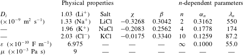
 $\unicode[STIX]{x1D701}_{1}=\unicode[STIX]{x1D701}_{2}=\unicode[STIX]{x1D701}$. Table 1 summarizes the physical properties of electrolyte solutions, electrolyte-related dimensionless parameters (
 $\unicode[STIX]{x1D712}$ and
 $\unicode[STIX]{x1D6FD}$) used in the present study and typical values for
 $n$-dependent dimensionless parameters (
 $\unicode[STIX]{x1D6FC}_{n}$ and
 $\unicode[STIX]{x1D706}_{n}$).
Physical properties and typical values for  $n$-dependent parameters. Here, the solvent properties are taken from those of water, and the ion diffusivities are taken at infinite dilution in water at
 $T\simeq 298~\text{K}$. In addition,
 $\unicode[STIX]{x1D6FC}_{n}$ and
 $\unicode[STIX]{x1D706}_{n}$ are determined at fixed values of
 $h_{0}/a=0.1$,
 $N_{\infty }=1~\text{mM}$ and
 $U_{z}=10~\unicode[STIX]{x03BC}\text{m}~\text{s}^{-1}$.

4.1 Squeeze-out flow and dissipative hydrodynamic pressure
Based on the derivation in § 3, we see that the electroviscous effect has two consequences: the first is to modify the flow field (i.e. the velocity and pressure distributions), and the second is to result in an extra dissipative force (i.e. the electroviscous coefficient). In the following, we present a detailed discussion of the electroviscous effects with reference to these two consequences. These two consequences are closely related, and the modification of the flow field is the direct reason for the dissipation enhancement. The discussion of the two consequences leads to a complete understanding of the electroviscous effect. This is different from most of the previous research, which only focused on the electroviscous coefficient.
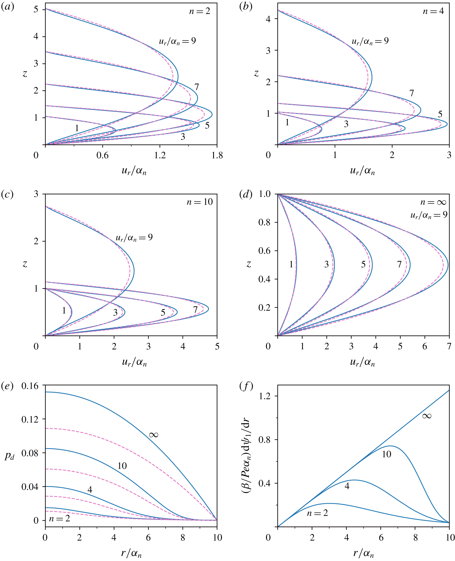
Electroviscous-effect-modified velocity profiles of the NaCl solution inside the gap between the tip and substrate for  $\unicode[STIX]{x1D701}_{1}=\unicode[STIX]{x1D701}_{2}=\unicode[STIX]{x1D701}=-4$ and
 $K=\unicode[STIX]{x1D705}h_{0}=2$. The results of four tip profiles are shown in (a)
 $n=2$ (i.e. spherical tip), (b)
 $n=4$, (c)
 $n=10$ and (d)
 $n=\infty$ (i.e. flat tip). Panels (e,f) respectively plot the dissipative hydrodynamic pressure and induced streaming potential field for the four tip profiles. The solid (dashed) lines correspond to the results with (without) the electroviscous effect. The calculation parameters are found in table 1.

To have an intuitive understanding of the electroviscous effects on the flow field, we plot the velocity profiles of the squeezing flow of the NaCl solution for various tip profiles in figure 2. It is clear from figures 2(a)–2(d) that the flow profiles inside the gap between the tip and substrate during the squeeze out of electrolyte solution are modified by the electroviscous effect. Generally, the velocity profiles with the electroviscous effect look sharper as compared to those without the electroviscous effect. This is because, under the electroviscous effect, there is a resistive electrostatic body force which tends to slow down the liquid flow in EDLs near the surfaces, while the requirement of mass conservation tends to accelerate the liquid flow in the middle portion of the gap.
Then, we elaborate on the effect of the tip profile on the velocity profiles. For the tip profile with a finite value of  $n$, such as
 $n=2$, 4 and 10, the velocity profile expands along the gap height direction as the radial location increases. The difference is that such expansion of the velocity profile takes place gradually for the sharp tip profile, which has a small value of
 $n$, but abruptly for the blunt tip with a large value of
 $n$. This feature is found to be reasonable on looking at the tip profiles schematically shown in figure 1(b). For an infinite value of
 $n$, namely,
 $n=\infty$, the tip is flat and there is apparently no expansion of velocity along the gap height direction. At a same radial location (
 $r/\unicode[STIX]{x1D6FC}_{n}$), for a smaller value of
 $n$, the velocity profile is more expanded along the gap height direction, while the maximum velocity (
 $u_{r}/\unicode[STIX]{x1D6FC}_{n}$) at the gap centre is much lower.
The coupling between the electroviscous effect and the tip profile has an intriguing impact on the velocity profiles. For the tip profiles with a finite value of  $n$, such as
 $n=2$, 4 and 10, the modification of velocity profile due to the electroviscous effect is the most pronounced at a specific radial location (e.g.
 $r/\unicode[STIX]{x1D6FC}_{n}=3$, 5, 7 approximately for
 $n=2$, 4, 10, respectively), while for the flat tip (
 $n=\infty$), the modification of the velocity profiles becomes increasingly prominent as the radial location increases. These features can be understood by looking at the induced streaming potential field distribution along the radial direction shown in figure 2(f), since a higher electric field strength produces a higher resistive body force in the EDL to modify the flow field. The induced electric field shown in this plot is defined as
 $(\unicode[STIX]{x1D6FD}/Pe\unicode[STIX]{x1D6FC}_{n})\,\text{d}\unicode[STIX]{x1D713}_{1}/\text{d}r$ to directly compare its relative magnitude for varying
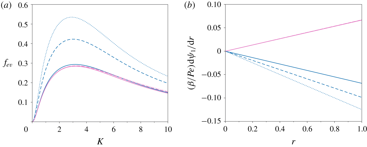
 $n$. Clearly, the induced electric field for the flat tip increases linearly and monotonically with increasing radial location, while the induced electric fields for the non-flat tips show local maxima roughly at
 $r/\unicode[STIX]{x1D6FC}_{n}=3$, 5 and 7 for
 $n=2$, 4, and 10 respectively, and decrease asymptotically to zero as
 $r/\unicode[STIX]{x1D6FC}_{n}\rightarrow \infty$. Therefore, for the flat tip, the electroviscous effect is expected to augment along the radial direction monotonically, while for the three non-flat tips the electroviscous effect is expected to have local maxima and then vanish as
 $r/\unicode[STIX]{x1D6FC}_{n}\rightarrow \infty$. These characteristics are consistent with the velocity profiles shown in figures 2(a)–2(d). The difference between the flat tip and non-flat tips can be understood more intuitively by considering the extent of the overlap of the tip EDL and substrate EDL. It is known that the EDL overlap induces the local charge density and the streaming electric field, and the interaction of these two produces an electrostatic body force to resist the squeeze out of the solution. For a flat tip, the EDL overlap is uniform in the radial direction, and thus so is the electroviscous effect. Yet, for the non-flat tips, the EDL overlap gradually vanishes as the radial location increases, and so does the electroviscous effect.
The pressure distributions for the four tip profiles are displayed in figure 2(e). It is clear that the pressure for a blunt tip (large  $n$) is higher than that for a sharp tip (small
 $n$). We also observe that the radial pressure gradient for the flat tip and the non-flat tips exhibits strikingly different behaviours. For the flat tip, the pressure gradient increases monotonically along the radial direction, while for the non-flat tips the pressure gradient increases with
 $r/\unicode[STIX]{x1D6FC}_{n}$ first to a maximum and then decreases to zero as
 $r/\unicode[STIX]{x1D6FC}_{n}\rightarrow \infty$. Other than modifying the velocity profiles, the electroviscous effect also modifies the dissipative hydrodynamic pressure distribution, as shown in figure 2(e). Generally, the electroviscous effect enhances the pressure for all tip profiles. This indicates that the dissipative hydrodynamic force experienced by the tip is also enhanced, and such enhancement of dissipative force due to the electroviscous effect is the focus of the present investigation. The electroviscous coefficient defined in (3.62) quantifies this effect and the following discussion concentrates on the characteristics of the electroviscous coefficient.
Variation of the electroviscous coefficient with electrokinetic separation  $K=\unicode[STIX]{x1D705}h_{0}$ for five
 $\unicode[STIX]{x1D701}$ potentials (
 $-1$,
 $-2$,
 $-4$,
 $-8$ and
 $-16$) in the NaCl solution. The plot contains the results of two tip profiles which are differentiated by two colours, the blue lines correspond to the flat tip (
 $n=\infty$) while the magenta lines correspond to the spherical tip (
 $n=2$). For each
 $\unicode[STIX]{x1D701}$ value, there is a prediction using the constant-charge boundary (solid line) and a prediction using the constant-potential boundary (dashed line). The logarithmic scale for
 $K$ is used to see the detail for very small separation.

4.2 Electroviscous effect and its dependence on various electrokinetic factors
Figure 3 presents the variation of the electroviscous coefficient with the dimensionless separation (or electrokinetic separation  $K=\unicode[STIX]{x1D705}h_{0}$) for a flat tip and a spherical tip. As is seen from the plot, the characteristics of the electroviscous coefficient with respect to the electrokinetic separation
 $K$ and
 $\unicode[STIX]{x1D701}$ potential are similar for the two tip profiles. For either tip profile, the characteristics of the electroviscous coefficient can be divided into two regimes: (i) When the
 $\unicode[STIX]{x1D701}$ value is below a particular value (approximately
 $-4$), the electroviscous coefficient increases with the
 $\unicode[STIX]{x1D701}$ value in the entire range of electrokinetic separation (viz.
 $K$ from 0 to infinity). In addition, the maximal electroviscous coefficient is achieved roughly at a particular electrokinetic separation for each tip profile, regardless of the
 $\unicode[STIX]{x1D701}$ value. Such electrokinetic separation
 $K$ is approximately 3 for the flat tip and 1 for the spherical tip. (ii) As the
 $\unicode[STIX]{x1D701}$ value increases further beyond
 $-4$, the characteristics of the electroviscous effect differ from regime (i). There is a range of electrokinetic separations in which the electroviscous coefficient shows an inverse dependence on the
 $\unicode[STIX]{x1D701}$ value as compared to regime (i), e.g. as
 $K\geqslant 3$ for the flat tip and
 $K\geqslant 1$ for the spherical tip, we see that the magnitude of the electroviscous coefficient is ranked in reverse order with respect to increasing the
 $\unicode[STIX]{x1D701}$ value. In addition, the electrokinetic separation corresponding to the maximal electroviscous effect reduces significantly as the
 $\unicode[STIX]{x1D701}$ value increases. Furthermore, the shape of the electroviscous coefficient profiles for the
 $\unicode[STIX]{x1D701}$ value beyond
 $-8$ is quite similar, with only a shift of the profile location towards the reducing
 $K$ direction.
Next, we discuss the effects of the boundary condition of the PB equation on the electroviscous coefficient. There are typically two types of boundary condition for the PB equation, i.e. the CP boundary in (3.22) and the CC boundary in (3.23). For each tip profile under a given  $\unicode[STIX]{x1D701}$ value, there is one prediction from the CP boundary and one prediction from the CC boundary, as shown in figure 3. It is widely accepted that the CC and CP boundaries become identical as the electrokinetic separation increases to the extent of no overlap of the tip EDL and substrate EDL (Russel et al. Reference Russel, Saville and Schowalter1989; Masliyah & Bhattacharjee Reference Masliyah and Bhattacharjee2006; Israelachvili Reference Israelachvili2011). This feature is apparently reflected by the figure in which the solid lines (CC boundary) and dashed lines (CP boundary) overlap for the large electrokinetic separation. The CC and CP boundaries are two extreme conditions, and the practical boundary generally lies in between the two conditions (Israelachvili Reference Israelachvili2011; Montes Ruiz-Cabello et al. Reference Montes Ruiz-Cabello, Trefalt, Maroni and Borkovec2014; Zhao et al. Reference Zhao, Ebeling, Siretanu, van den Ende and Mugele2015). In comparison with the CC and CP, which fix the surface charge density and surface potential respectively, the boundary condition assuming a separation-dependent surface charge or potential proves to be more realistic and practical, and is typically called the charge regulation boundary (Montes Ruiz-Cabello et al. Reference Montes Ruiz-Cabello, Trefalt, Maroni and Borkovec2014; Zhao et al. Reference Zhao, Ebeling, Siretanu, van den Ende and Mugele2015). Yet, the formulation of the charge regulation boundary requires a priori knowledge of the surface chemistries which are responsible for the charging of the solid surface, and thus are quite involved and tedious. Hence, the present study only considers CC and CP boundaries, and one would expect that the CR boundary prediction should not be different from the CC and CP predictions significantly since theoretically it stays in between the CC and CP predictions and the gap between the two predictions is not significantly large. Accordingly, one can conclude that the electroviscous coefficient is insensitive to the CR and thus so is the dissipative hydrodynamic force. This assertion is straightforward for large electrokinetic separations since the difference between CC and CP boundaries disappears, as suggested by the preceding discussion. In principle, with decreasing electrokinetic separation, the difference between the CC and CP boundary predictions would become more pronounced because of the heavy interaction between the ion clouds in the EDLs close to the tip and substrate surfaces. However, in reality, for very small electrokinetic separations (
 $K=\unicode[STIX]{x1D705}h_{0}\ll 1$) the electroviscous coefficients predicted from the CC and CP boundaries would approach each other. Actually, in this case, the ion concentration and EDL potential weakly vary with the
 $z$ direction. Thus, the EDL charge density measured by
 $c_{1}(r)/h^{2}(r)$ would approach zero (see (3.38)) and so would the electroviscous coefficient (see (3.62)), regardless of the boundary conditions. This implies that, for very small electrokinetic separations, the difference in the dissipative hydrodynamic force predicted from the CC and CP boundaries disappears.
An unexpected observation from figure 3 is that the difference in the electroviscous coefficient predicted from the CC and CP boundaries becomes smaller as the magnitude of the  $\unicode[STIX]{x1D701}$ potential increases. This is in contradiction with the conclusion for the case of the conservative EDL interaction force between two surfaces. Usually, in the prediction of the conservative EDL interaction force, the difference in force predicted from the CC and CP boundaries becomes more pronounced as the magnitude of the
 $\unicode[STIX]{x1D701}$ value increases. To summarize, the difference in the dissipative electroviscous interaction force predicted from the CC and CP boundaries is mitigated by the high
 $\unicode[STIX]{x1D701}$ values, but the difference in the conservative EDL interaction force predicted from the CC and CP boundaries is intensified by the high
 $\unicode[STIX]{x1D701}$ values. This striking characteristic highlights the inherent difference between the conservative EDL force and dissipative electroviscous force. In what follows, we would illuminate the physical rationale regarding such a difference. For large electrokinetic separations, both the conservative EDL force and dissipative hydrodynamic force are insensitive to the CR due to the equivalence of the CC and CP boundary conditions. However, for small electrokinetic separations, the dissipative hydrodynamic force has been shown to be insensitive to the boundary conditions, while the conservative EDL force is strongly dependent on the boundary conditions. Actually, for a given electrokinetic separation,
 $K$, the EDL force per unit area is independent of the
 $z$ location (Masliyah & Bhattacharjee Reference Masliyah and Bhattacharjee2006) and thus can be calculated on the surfaces as
 $p_{EDL}=2[\cosh (\unicode[STIX]{x1D701})-1]-q^{2}$, where the first and second terms on the right-hand side are the osmotic pressure and the Maxwell stress, respectively. Note that the osmotic pressure for the CP boundary and the Maxwell stress for the CC boundary are fixed. As the electrokinetic separation decreases to a very small value, the EDLs can fully overlap and thus the EDL potential almost becomes uniform along the
 $z$ direction. In this case, the surface charge density for the CP boundary condition decays to be infinitely small and so does the Maxwell stress, thus the EDL force predicted from the CP boundary condition tends to fixed values; whereas the magnitude of
 $\unicode[STIX]{x1D701}$ potential for the CC boundary condition becomes extremely large and so does the osmotic pressure, thus the EDL force predicted from the CC boundary condition tends to infinity (probably unphysical). Therefore, a significant difference in the conservative EDL forces predicted from the CC and CP boundary conditions is present within small electrokinetic separations. Furthermore, such difference is expected to be more significant as the
 $\unicode[STIX]{x1D701}$ potential increases.
The preceding discussion of figure 3 implies that the variation of the electroviscous coefficient with the  $\unicode[STIX]{x1D701}$ potential is not monotonic. To see this trend more straightforwardly, we depict the variation of the electroviscous coefficient with the
 $\unicode[STIX]{x1D701}$ potential under several values of electrokinetic separation in figure 4 for the two tip profiles. The figure clearly indicates a non-monotonic variation of the electroviscous coefficient with the
 $\unicode[STIX]{x1D701}$ potential, and for a given tip profile, there is one specific value of the
 $\unicode[STIX]{x1D701}$ potential for each electrokinetic separation under which the electroviscous coefficient is maximal. The characteristics of the electroviscous coefficient are similar for a flat tip and a spherical tip. Generally, the characteristics of the electroviscous coefficient can be divided into two regimes depending on the magnitude of
 $K$: (i) When the electrokinetic separation
 $K$ is larger than a critical value (approximately 4 for the flat tip and 1 for the spherical tip), the electroviscous coefficient decreases with increasing
 $K$ in the entire range of
 $\unicode[STIX]{x1D701}$ potential (viz. 0 to infinity). In addition, the
 $\unicode[STIX]{x1D701}$ potential values corresponding to the maximal electroviscous effect are not very different for various separations. (ii) When
 $K$ is below the critical value, the characteristics of the electroviscous effect are different. There is an apparent increase of the
 $\unicode[STIX]{x1D701}$ potential value corresponding to the highest electroviscous coefficient as the electrokinetic separation
 $K$ reduces, and the maximal electroviscous coefficient tends to saturate to one particular value (e.g. approximately 0.47 for the flat tip) irrespective of the value of electrokinetic separation.
Variation of the electroviscous coefficient with the  $\unicode[STIX]{x1D701}$ potential under six electrokinetic separations (
 $K=\unicode[STIX]{x1D705}h_{0}=0.1$, 1, 2, 4, 8, 16) in the NaCl solution for a flat tip (solid lines) and a spherical tip (dashed lines).
 $K$ increases sequentially along the direction indicated by the red arrow.

It is noted from the analytical solution that the electroviscous coefficient is a function of five variables, namely, the electrokinetic separation ( $K$) and the
 $\unicode[STIX]{x1D701}$ potential, the tip profile (
 $n$) and the electrolyte-related parameters (
 $\unicode[STIX]{x1D6FD}$ and
 $\unicode[STIX]{x1D712}$). Figures 3 and 4 particularly discuss the effects of
 $K$ and
 $\unicode[STIX]{x1D701}$, and the important finding is that the electroviscous effect is maximal in a certain
 $K$–
 $\unicode[STIX]{x1D701}$ domain. This will be more clearly demonstrated later in figure 7. In the following, we expatiate the reason for the maximal electroviscous coefficient at one particular value of the
 $\unicode[STIX]{x1D701}$ potential for a given electrokinetic separation, and discuss the effects of the tip profile and the electrolyte on the electroviscous effect in succeeding subsections.
The induced streaming potential field for the flat tip in the NaCl solution as  $K=\unicode[STIX]{x1D705}h_{0}=1$. (a) The contour plot of the magnitude of the induced electric potential field (
 $A(r)$ or equivalently
 $-\unicode[STIX]{x1D6FD}I_{2}/(\unicode[STIX]{x1D6FD}I_{1}+I_{3})$) in the
 $\unicode[STIX]{x1D701}$–
 $r$ domain; (b) the contour plot of the convection current (
 $-\unicode[STIX]{x1D6FD}I_{2}$) in the
 $\unicode[STIX]{x1D701}$–
 $r$ domain; (c) the contour plot of electric conductivity (
 $\unicode[STIX]{x1D6FD}I_{1}+I_{3}$) in the
 $\unicode[STIX]{x1D701}$–
 $r$ domain; (d) the contour plot of
 $-A(r)c_{1}(r)$ in the
 $\unicode[STIX]{x1D701}$–
 $r$ domain.

The electroviscous coefficient for four different tip profiles in the NaCl solution as  $\unicode[STIX]{x1D701}=-4$. The four curves are corresponding to four power-law indices of tip profile (
 $n=2$, 4, 10,
 $\infty$) in figure 1(b). Particularly,
 $n=2$ corresponds to a spherical tip and
 $n=\infty$ corresponds to a flat tip. The tip becomes blunter as the index
 $n$ increases. The insets show the region of EDL overlap for two limiting cases (
 $n=2$ and
 $\infty$).

The presence of the highest electroviscous coefficient at one specific value of the  $\unicode[STIX]{x1D701}$ potential for a given electrokinetic separation,
 $K=\unicode[STIX]{x1D705}h_{0}$, seems counter-intuitive, since the conventional view is that the increase of the
 $\unicode[STIX]{x1D701}$ potential absolutely enhances both the induced electric field and the local charge density inside the EDL, and then the electroviscous effect would be enhanced accordingly. According to (3.62), the electroviscous coefficient is defined as an integral related to the product of
 $A(r)$ and
 $-c_{1}(r)/h^{2}(r)$, which essentially represent the induced streaming electric field and the EDL charge density, respectively. Our calculations indicate that, for a given electrokinetic separation,
 $K$, the induced electric field
 $A(r)$ is the highest under one specific value of the
 $\unicode[STIX]{x1D701}$ potential. To see this effect clearly, we plot the contour of the induced electric field of a flat tip in the
 $\unicode[STIX]{x1D701}$ potential–radial location (
 $\unicode[STIX]{x1D701}$–
 $r$) domain in figure 5(a) for
 $K=1$, which corresponds to the case of
 $K=1$ in figure 4. At a given radial location, it is seen that the induced electric field is the highest at a
 $\unicode[STIX]{x1D701}$ potential of approximately
 $-3$, and becomes negligible as the
 $\unicode[STIX]{x1D701}$ potential either reduces to zero or becomes very large. For a given
 $\unicode[STIX]{x1D701}$ potential, the electric field however increases monotonically along the radial direction.
Basically, the streaming potential field is induced to cause a conductive transport of charge (conduction current) to balance the convective transport of charge (streaming current) due to the squeeze-out flow, as shown in (3.46). According to (3.48), the resulting electric field  $A(r)=(\unicode[STIX]{x1D6FD}/Pe)\,\text{d}\unicode[STIX]{x1D713}_{1}/\text{d}r$ can be expressed as
 $-\unicode[STIX]{x1D6FD}I_{2}/(\unicode[STIX]{x1D6FD}I_{1}+I_{3})$, in which the numerator denotes the convection current due to the squeeze-out flow and the denominator denotes the electric conductivity. To better understand the induced streaming potential field in figure 5(a), we also present the contour plots of the numerator (
 $-\unicode[STIX]{x1D6FD}I_{2}$) and the denominator (
 $\unicode[STIX]{x1D6FD}I_{1}+I_{3}$) in figures 5(b) and 5(c), respectively. Clearly, the convective current increases with the increase of either the
 $\unicode[STIX]{x1D701}$ potential or the radial location, since the charge density inside the EDL increases with the increase of the
 $\unicode[STIX]{x1D701}$ potential and the liquid velocity increases with the increase of the radial location. More precisely, it is observed that the convective current scales linearly with the radial location under a given
 $\unicode[STIX]{x1D701}$ potential. This is simply because the local radial velocity increases linearly along the radial direction for the flat tip.
The effective electric conductivity expressed by the denominator  $\unicode[STIX]{x1D6FD}I_{1}+I_{3}$ in figure 5(c) shows a rather nonlinear dependence on the magnitude of
 $\unicode[STIX]{x1D701}$ potential. For a low value of
 $\unicode[STIX]{x1D701}$ potential, the conductivity increases very slowly, while as the
 $\unicode[STIX]{x1D701}$ potential increases beyond a particular value (approximately 12 in this case), the conductivity increases dramatically. For a flat tip considered here, the electric conductivity distributes evenly along the radial direction, and such feature is clearly shown in the figure.
By jointly analysing figures 5(b) and 5(c), one can see that the induced electric field attaining the maximal value under one specific  $\unicode[STIX]{x1D701}$ potential for a given electrokinetic separation,
 $K$, is quite straightforward. Generally, the increase of the
 $\unicode[STIX]{x1D701}$ potential leads to the increment of both numerator (convection current) and denominator (electric conductivity). However, as the
 $\unicode[STIX]{x1D701}$ potential value is below a particular value (
 $-3$ in this case), the increase of numerator is dominant, and then the induced electric field increases with the increasing
 $\unicode[STIX]{x1D701}$ potential; on the contrary, as the
 $\unicode[STIX]{x1D701}$ potential is beyond such particular value, the increase of denominator is dominant and then the induced electric field decreases with the increasing
 $\unicode[STIX]{x1D701}$ potential. Apparently, the induced electric field attains the maximum value under this particular
 $\unicode[STIX]{x1D701}$ potential.
Finally, we show the contour plot of  $-A(r)c_{1}(r)$, namely, the product of the induced streaming electric field and the EDL charge density (since in current case
 $h(r)\equiv 1$), in figure 5(d), since it provides a piece of direct evidence for the characteristics of the electroviscous coefficient as suggested by (3.48). It is clear that the characteristics of
 $-A(r)c_{1}(r)$ are very similar to
 $-A(r)$. However, the maximal magnitude of
 $-A(r)c_{1}(r)$ at a given radial location shifts to a high
 $\unicode[STIX]{x1D701}$ potential of approximately
 $-7$, which is then consistent with figure 4 in which, for
 $K=1$, the maximal electroviscous coefficient is achieved under
 $\unicode[STIX]{x1D701}\approx -7$ for the flat tip.
4.3 Influence of tip profile on electroviscous effect
Figure 6 illustrates the effect of the tip profile on the electroviscous coefficient, and the tip profile effect is apparently non-trivial. The general trend from this figure is that, as the tip becomes blunter, namely, as  $n$ increases, the range of electrokinetic separation (
 $K=\unicode[STIX]{x1D705}h_{0}$) in which the electroviscous effect is prominent becomes more expanded. Such trend makes sense because, at a given electrokinetic separation,
 $K$, a bunter tip has a much larger region of EDL overlap along the radial direction (see insets in figure 6) by noticing that the local tip–substrate gap,
 $h(r)$, decreases with increasing
 $n$ (see figure 1b) and the EDL thickness (measured by the Debye length) is independent of
 $r$ location. Due to the same reason, the decaying of the electroviscous coefficient with respect to increasing the electrokinetic separation is much slower as the tip becomes blunter. For a given tip profile, there is one specific value of electrokinetic separation at which the electroviscous coefficient is the strongest. This feature has been previously shown in figure 3. Additionally, as the tip becomes blunter, the electrokinetic separation corresponding to the maximal electroviscous coefficient and the corresponding maximal electroviscous coefficient increases concurrently. The effect of the tip profile on the magnitude of the electroviscous coefficient is complex. Depending on the magnitude of electrokinetic separation, there are three scenarios: First, for electrokinetic separation
 $K\gtrsim 3$, the electroviscous coefficient increases as the tip profile becomes blunter. Second, for electrokinetic separation
 $K\lesssim 0.5$, the dependence of the electroviscous coefficient on the tip profile is reversed as compared to the first scenario. Third, in an intermediate range of electrokinetic separation (
 $0.5\lesssim K\lesssim 3$), any two of the four profiles in the figure cross over each other, suggesting an equal electroviscous coefficient at a particular value of electrokinetic separation. Essentially, the electroviscous coefficient is the ratio of the electroviscous force (i.e.
 $F_{z,d}-F_{z,d0}$) to the hydrodynamic force without the EDL effect (i.e.
 $F_{z,d0}$). Hence, the presence of the preceding different scenarios is due to the competition of two effects: First, as
 $n$ increases, the local electrokinetic separation,
 $Kh(r)$, decreases, which can enhance the streaming electric field (figure 2f) and the EDL charge density. These tend to enhance the electroviscous force and thus the electroviscous coefficient. Second, with the increase of
 $n$ the dissipative hydrodynamic force without the EDL effect potentially increases and thus the electroviscous coefficient decreases. For very small electrokinetic separations, the second effect is dominant, whereas for large electrokinetic separations the first effect is dominant, leading to the characteristics shown in figure 6.
In figure 6, one also sees that when the power-law index  $n$ is in the range of 2–10, the difference in the electroviscous coefficient profiles is noticeable, while when
 $n$ increases beyond 10, the electroviscous coefficient profiles are similar. This is because the tip profile changes dramatically when
 $n<10$, but does not when
 $n>10$; see figure 1(b) for clarification. The current model addresses the tip profile effect with a power-law index
 $n$, and this provides a quantitative characterization of the tip profile effect on the electroviscous coefficient. It is evident that our new model is more general, since the existing literature studies either consider a plate–plate (
 $n=\infty$ in our model) configuration or a sphere–plate (
 $n=2$ in our model) configuration.
Figure 7 shows the contour plots of the electroviscous coefficient for four tip profiles in the  $\unicode[STIX]{x1D701}$–
 $K$ domain, and these plots present a complete description of the dependence of the electroviscous coefficient on the
 $\unicode[STIX]{x1D701}$ potential and electrokinetic separation. Generally, the characteristics of the contour plots for four tip profiles are similar. For each tip profile, there are two tilted zones in which the electroviscous coefficient is large, and these two zones correspond to
 $\unicode[STIX]{x1D701}>0$ and
 $\unicode[STIX]{x1D701}<0$, respectively. Outside these two zones, the electroviscous coefficient is negligibly small. Although appearing similar in shape, the two zones of massive electroviscous effect gradually shift towards the increasing
 $K$ direction as the tip becomes blunter. We also see that the two zones of massive electroviscous effect are asymmetric with respect to
 $\unicode[STIX]{x1D701}=0$ since the electroviscous coefficient in the zone of
 $\unicode[STIX]{x1D701}<0$ is generally higher than that in the zone of
 $\unicode[STIX]{x1D701}>0$. Such asymmetry in the two zones of massive electroviscous effect is due to the difference in the diffusivity of cations and anions, as elaborated on in the later discussion. Furthermore, in the two zones of massive electroviscous effect, the maximal electroviscous effect can be achieved with a small electrokinetic separation/a high
 $\unicode[STIX]{x1D701}$ or a large electrokinetic separation/a low
 $\unicode[STIX]{x1D701}$. It can be seen that for a given tip profile and a given sign of
 $\unicode[STIX]{x1D701}$ the maximal electroviscous effect is achieved as the
 $\unicode[STIX]{x1D701}$ and
 $\log _{10}(K)$ satisfy a certain linear relationship. It is obvious that with the contour plots in figure 7, the characteristics of the electroviscous coefficient shown in figures 3, 4 and 6 are readily understandable.
Contour plots of the electroviscous coefficient of NaCl solution in the  $\unicode[STIX]{x1D701}$–
 $K$ domain for four tip profiles, (a)
 $n=2$; (b)
 $n=4$; (c)
 $n=10$ and (d)
 $n=\infty$.

4.4 Influence of electrolyte type on electroviscous effect
In this subsection, the dependence of the electroviscous effect on the electrolyte is discussed. To this end, figure 8 presents the electroviscous coefficient for a flat tip in three different electrolyte solutions, i.e. LiCl, NaCl and KCl. In the case of the tip and substrate being both negatively charged, figure 8(a) shows a clear dependence of the electroviscous effect on the electrolyte. For the three electrolytes considered, the electroviscous coefficient increases according to  $\text{LiCl}>\text{NaCl}>\text{KCl}$. However, in the case of the tip and substrate being both positively charged, the electroviscous coefficient is negligibly dependent on the electrolyte. These are quite interesting results which indicate that the extent of the dependence of the electroviscous effect on the electrolyte is controlled by the polarity of the
 $\unicode[STIX]{x1D701}$ potential. Physically, the electroviscous effect arises from the interaction of the induced electric field and the charge density in the EDL, and thus the characteristics of the electroviscous coefficient in figure 8(a) can be understood by analysing the characteristics of the charge density in the EDL and the induced electric field. The charge densities in the EDL for three electrolytes are expected to be identical because of the same
 $\unicode[STIX]{x1D701}$ potential. Therefore, the characteristics of the electroviscous coefficient are primarily due to the induced streaming potential field. Figure 8(b) shows the streaming potential field for
 $K\approx 3$ which roughly corresponds to the maximal electroviscous effect. It is seen that for the negatively charged case, the induced electric field increases according to
 $\text{LiCl}>\text{NaCl}>\text{KCl}$, while in the positively charged case, the induced electric fields for three electrolytes are nearly the same. As previously discussed, the induced electric field can be seen as a ratio of the convection current to the local conductivity. For either a positively or negatively charged case, the magnitude of the convection current is the same for the three electrolytes since the flow field as well as the charged density is identical for the three electrolytes. Yet, for the electric conductivity, the situation differs for the positively charged case and the negatively charged case. In the negatively charged case, the conduction is mainly contributed by cations (
 $\text{Li}^{+}$,
 $\text{Na}^{+}$, and
 $\text{K}^{+}$). The diffusivity of these cations reduces according to
 $\text{Li}^{+}<\text{Na}^{+}<\text{K}^{+}$, and accordingly the conductivity is ranked as
 $\text{Li}^{+}<\text{Na}^{+}<\text{K}^{+}$. Therefore, the induced electric field would rank in an order which is inverse to the conductivity ranking, namely,
 $\text{Li}^{+}>\text{Na}^{+}>\text{K}^{+}$. In the positively charged case, the conduction is mostly contributed by the anion
 $\text{Cl}^{-}$ which is identical for three electrolytes, and accordingly the conductivity for three electrolytes is not significantly different. Then, the induced electric fields for three electrolytes would be nearly the same in the positively charged case.
The electrolyte dependence of the electroviscous effect. (a) The electroviscous coefficient for a flat tip in three different electrolytes (LiCl, NaCl and KCl) and (b) the induced streaming potential field for  $K=\unicode[STIX]{x1D705}h_{0}\approx 3$. Different electrolytes are differentiated by different line styles: solid lines (KCl), dashed lines (NaCl) and dotted lines (LiCl). The polarity of
 $\unicode[STIX]{x1D701}$ is distinguished by different colours: blue (
 $\unicode[STIX]{x1D701}=-4$), magenta (
 $\unicode[STIX]{x1D701}=4$).

The significance of the results in figure 8 is that the electroviscous coefficient for a given  $\unicode[STIX]{x1D701}$ value is determined by the induced streaming potential field, and ultimately by the effective conductivity of counterions in the EDL. This concept provides a convenient and efficient approach to rank the electroviscous effect by electrolyte under a given
 $\unicode[STIX]{x1D701}$ value by comparing the counterion conductivity in the EDL.
For a complete understanding of the electrolyte effect on the electroviscous coefficient, figure 9 presents the contour plots of electroviscous coefficient of three electrolytes in the  $\unicode[STIX]{x1D701}$–
 $K$ domain for a flat tip. The result for NaCl has been shown in figure 7(d) and thus is omitted here. For KCl, we see a rather symmetric distribution of two zones of massive electroviscous effect with respect to
 $\unicode[STIX]{x1D701}=0$ in figure 9(a), while for NaCl and LiCl the two zones of massive electroviscous effect are asymmetric since the electroviscous coefficient for
 $\unicode[STIX]{x1D701}<0$ is generally higher than that for
 $\unicode[STIX]{x1D701}>0$. This is expected to be due to the negative
 $\unicode[STIX]{x1D712}$ of electrolytes by following the same reasoning as figure 8. It is seen that the extent of asymmetry in the two zones of heavy electroviscous effect is ranked as
 $\text{LiCl}>\text{NaCl}>\text{KCl}$. This is due to the fact that the diffusivity difference between cations and anions (or the magnitude of
 $\unicode[STIX]{x1D712}$) increases according to
 $\text{LiCl}>\text{NaCl}>\text{KCl}$. We also observe the reoccurring characteristics in figure 8 that for
 $\unicode[STIX]{x1D701}>0$, the electroviscous effect of three electrolytes is not much different, while for
 $\unicode[STIX]{x1D701}$¡0, the electroviscous effect of three electrolytes is dramatically different and is clearly ranked as
 $\text{LiCl}>\text{NaCl}>\text{KCl}$. The reason for this behaviour has been elaborated in the discussion of figure 8. The contour plots in figure 9 not only present a clear dependence of the electroviscous effect on
 $\unicode[STIX]{x1D701}$ potential and electrokinetic separation
 $K$, but also can be used for the fast estimation of the value of electroviscous coefficient under a given set of conditions, namely,
 $\unicode[STIX]{x1D701}$,
 $K$ and type of electrolyte.
Contour plots of the electroviscous coefficients for (a) KCl solution and (b) LiCl solution in the  $\unicode[STIX]{x1D701}$–
 $K$ domain for a flat tip.

Note that there are two dimensionless parameters distinguishing one electrolyte from another, i.e.  $\unicode[STIX]{x1D712}$ and
 $\unicode[STIX]{x1D6FD}$ (see (3.13c) and (3.32) respectively). The difference in ion diffusivity would only influence these two parameters. The intrinsic Péclet number
 $\unicode[STIX]{x1D6FD}$ characterizes the average diffusion coefficient of cations and anions, while
 $\unicode[STIX]{x1D712}$ characterizes the difference in the diffusivity between cations and anions. Therefore, the effects of electrolytes on the electroviscous coefficient are well reflected by
 $\unicode[STIX]{x1D712}$ and
 $\unicode[STIX]{x1D6FD}$. In addition to the three alkali-halide electrolytes, we would provide a more comprehensive understanding of the electrolyte effect on the electroviscous coefficient. For this purpose, we present the dependence of the electroviscous coefficient on
 $\unicode[STIX]{x1D712}$ and
 $\unicode[STIX]{x1D6FD}$ within
 $-1\leqslant \unicode[STIX]{x1D712}\leqslant 1$ and
 $\unicode[STIX]{x1D6FD}=0.1{-}0.9$ by noting that for a typical symmetric 1 : 1 electrolyte,
 $-1<\unicode[STIX]{x1D712}<1$ and
 $O(0.1)\lesssim \unicode[STIX]{x1D6FD}<1$. Figure 10 displays the corresponding results for
 $n=2$,
 $\unicode[STIX]{x1D701}=-4$ and
 $K=\unicode[STIX]{x1D705}h_{0}=2$. It is apparent from figure 10 that the electroviscous coefficient decreases with increasing
 $\unicode[STIX]{x1D712}$ and such a decrease becomes more significant at
 $\unicode[STIX]{x1D712}<-0.5$. This behaviour supports the preceding assertion that the electroviscous coefficient is ultimately determined by the conductivity of the counterion in the EDL. In fact, for a given value of the intrinsic Péclet number
 $\unicode[STIX]{x1D6FD}$ (or average ion diffusivity
 $D$), a decrease in
 $\unicode[STIX]{x1D712}$ leads to a decrease in the diffusivity of cations (i.e. counterions) in the EDL, and thus leads to a decrease in the conductivity of counterions in the EDL. In addition, one can clearly observe that the electroviscous coefficients for the hypothetical case of
 $\unicode[STIX]{x1D712}=0$ assumed in previous work (Muller Reference Muller1990) could heavily deviate from those for the practical case of non-zero
 $\unicode[STIX]{x1D712}$ if
 $\unicode[STIX]{x1D712}$ significantly deviates from zero.
Electroviscous coefficient as a function of  $\unicode[STIX]{x1D712}$ for different
 $\unicode[STIX]{x1D6FD}$ (0.1, 0.3, 0.5, 0.7 and 0.9). The
 $\unicode[STIX]{x1D701}$ potential and electrokinetic separation are set to
 $\unicode[STIX]{x1D701}=-4$ and
 $K=\unicode[STIX]{x1D705}h_{0}=2$, respectively. The power-law index is set to
 $n=2$.

Figure 10 also indicates that the electroviscous coefficient increases with the increase of  $\unicode[STIX]{x1D6FD}$, and so does the dissipative hydrodynamic force. Practically, the increase of the intrinsic Péclet number implies the decrease of the average ion diffusivity, which gives rise to the decrease in ion conductivity and ion electrophoretic mobility in the EDL (since both ion conductivity and ion mobility are proportional to the ion diffusivity). Thus, it requires larger streaming electric fields driving the conduction current to balance the same streaming current (being independent of
 $\unicode[STIX]{x1D6FD}$). The above analyses provide a possible reason (at least partially) for the anomalously large electroviscous coefficient observed in the recent experiment (Liu et al. Reference Liu, Klaassen, Zhao, Mugele and van den Ende2018), i.e. the increase in the intrinsic Péclet number,
 $\unicode[STIX]{x1D6FD}$, or the decrease in the ion asymmetric ratio,
 $\unicode[STIX]{x1D712}$, more precisely, the decrease in the conductivity or electrophoretic mobility of counterions within the EDL. This makes sense since the accumulation of the counterions near the charged surfaces must lead to the decrease of the electrophoretic mobility of counterions from its bulk value (Qiao & Aluru Reference Qiao and Aluru2005; Bhadauria & Aluru Reference Bhadauria and Aluru2017).
5 Conclusions and outlook
The present work reports a detailed calculation of electroviscous effects in the squeezing flows of thin films of electrolyte solutions between two charged surfaces. We perform the calculation in the theoretical framework of electrokinetic transport phenomena by solving the Nernst–Planck equation for ion transport, the Poisson equation for electric potential distribution and the Navier–Stokes equation for liquid flow. With the lubrication approximation, we solved the three coupled equations under the conditions of low ionic Péclet number and a pseudo-steady state, which are justified for the dynamic AFM experiments by the order-of-magnitude analyses. The solution of the three equations gives rise to the interaction force between the two charged surfaces as well as the squeezing flow field of thin electrolyte solution films. Unlike the current literature, which treat the dissipative hydrodynamic force and the conservative EDL force individually, the present study naturally and self-consistently derives the total interaction force to be a superposition of one conservative EDL force, one conservative the van der Waals force and one dissipative hydrodynamic force enhanced by the electroviscous effect. The EDL and van der Waals forces are described by the well-known DLVO theory and have been well understood, while the electroviscous-effect-enhanced hydrodynamic force still lacks an in-depth understanding and thus is the focus of the present work. The major findings of the study are fivefold:
(I) The electroviscous effect is non-monotonic with respect to the variation of the  $\unicode[STIX]{x1D701}$ potential of the surface. For a given electrokinetic separation
 $K$, the electroviscous effect is the strongest under one specific value of
 $\unicode[STIX]{x1D701}$ potential, and reduces as the
 $\unicode[STIX]{x1D701}$ potential departs from this specific value. This feature is attributed to a competition between the increase of streaming current and the increase of electric conductivity when increasing the
 $\unicode[STIX]{x1D701}$ potential.
(II) The electroviscous effect is remarkably dependent on the shape of the surface profile. For a blunter tip file, the electroviscous effect is generally stronger, and is also pronounced in a much broader range of electrokinetic separations. This is due to the fact that the blunter tip has a much wider range of EDL overlap along the tip surface.
(III) The electroviscous effect modifies the velocity profiles inside the thin films to be much sharper. Such modification is an interplay of the electrostatic body force which resists the flow near the surface and the law of mass conservation which accelerates the flow in the bulk. The extent of modification is dependent on the tip profile, and generally a blunter tip leads to a more significant modification of the flow profiles.
(IV) The electroviscous effect is electrolyte dependent, and furthermore the extent of such dependency is affected by the polarity of surface charge or  $\unicode[STIX]{x1D701}$ potential. For three alkali-halide electrolytes considered in the study, i.e. KCl, NaCl and LiCl, the electroviscous effect becomes stronger in sequence for surfaces being negatively charged, while remaining nearly the same for surfaces being positively charged. Such distinct difference between the two oppositely charged cases can be understood in terms of the counterion conductivity in the EDL.
(V) The electroviscous effect is also dependent on the boundary conditions prescribed to the PB equation. Generally, for small electrokinetic separation with the EDL overlap, the CC boundary predicts a higher electroviscous coefficient than the CP boundary does, and such deviation becomes less evident as the  $\unicode[STIX]{x1D701}$ potential increases. For large electrokinetic separation without the EDL overlap, CC and CP boundary predictions coincide regardless of the
 $\unicode[STIX]{x1D701}$ values.
We further discuss the implications of the boundary conditions of the PB equation. For the conservative EDL force, it has been shown that CC and CP boundary predictions are not only dramatically different from each other, but also different significantly from the experiments, especially when the EDLs are heavily overlapped. A more realistic boundary condition for the PB equation is the charge regulation boundary, which self-consistently takes into account the confinement-induced shift of equilibria of surface chemistries (Montes Ruiz-Cabello et al. Reference Montes Ruiz-Cabello, Trefalt, Maroni and Borkovec2014; Zhao et al. Reference Zhao, Ebeling, Siretanu, van den Ende and Mugele2015). The CR boundary results in a separation-dependent surface charge density or  $\unicode[STIX]{x1D701}$ potential, which is clearly different from CC and CP boundaries, which fix the surface charge density and
 $\unicode[STIX]{x1D701}$ potential, respectively. It has been shown that the CR boundary can predict the conservative EDL force experiments quite accurately with the CC and CP boundary predictions being the upper and lower limits, respectively. However, the present study suggests that CC and CP boundary predictions of the dissipative electroviscous effect are not dramatically different. Although not calculating the electroviscous coefficient for the CR boundary, we expect that the CR prediction of electroviscous coefficient should not be far from the CC and CP predictions, since theoretically CC and CP boundaries are merely two limiting cases of the CR boundary. In summary, we can conclude that the conservative EDL force is very sensitive to the choice of boundary conditions for the PB equation, while the dissipative electroviscous force is apparently not. This highlights the inherent difference between the conservative EDL force and the dissipative electroviscous force.
The present model mimics the force measurements in the electrolyte environments with dynamic AFM and thus can serve as a theoretical foundation for these experiments. In the future, a comparison between the AFM measurements and our model will be instrumental in improving our understanding of the electroviscous dissipation in thin electrolyte films. Yet, one has to be alerted that our model could be too ideal to adequately describe the AFM experiments. For practical situations, one may wish to further account for other factors in the model development, such as ion-induced dielectric decrement (Levy, Andelman & Orland Reference Levy, Andelman and Orland2012; Zhao & Zhai Reference Zhao and Zhai2013), slippage on solid surfaces (Eijkel Reference Eijkel2007; Bocquet & Charlaix Reference Bocquet and Charlaix2010), finite size of ions (Levine & Bell Reference Levine and Bell1960; Borukhov, Andelman & Orland Reference Borukhov, Andelman and Orland1997), ion correlation (Bazant, Storey & Kornyshev Reference Bazant, Storey and Kornyshev2011; Laanait et al. Reference Laanait, Mihaylov and Hou2012), hydration of ions (Liu et al. Reference Liu, Zhao, Mugele and Ende2015) and last but not least the high oscillation frequency (i.e. namely large tip velocity). These effects could be of potential relevance under some extreme conditions, such as with extremely thin electrolyte films, highly charged surfaces, a high moving speed of the surfaces and high electrolyte concentration.
Acknowledgements
This work is supported by the National Natural Science Foundation of China (nos 51976157, 51721004) and the National Key Research and Development Program of China (no. 2017YFB0603500).
Declaration of interests
The authors report no conflict of interest.