1 Introduction
Interest in the flow around a circular disk goes back many years. Many experimental studies (see, e.g. Marshall & Stanton Reference Marshall and Stanton1931; Willmarth, Hawk & Harvey Reference Willmarth, Hawk and Harvey1964; Kuo & Baldwin Reference Kuo and Baldwin1967; Roos & Willmarth Reference Roos and Willmarth1971; Roberts Reference Roberts1973; Berger, Scholz & Schumm Reference Berger, Scholz and Schumm1990; Fernandes et al. Reference Fernandes, Risso, Ern and Magnaudet2007; Zhong & Lee Reference Zhong and Lee2012) and numerical calculations (see, e.g. Michael Reference Michael1966; Rimon Reference Rimon1969; Rivet et al. Reference Rivet, Henon, Frisch and d’Humieres1988; Fabre, Auguste & Magnaudet Reference Fabre, Auguste and Magnaudet2008; Shenoy & Kleinstreuer Reference Shenoy and Kleinstreuer2008; Auguste, Fabre & Magnaudet Reference Auguste, Fabre and Magnaudet2010; Chrust, Bouchet & Dušek Reference Chrust, Bouchet and Dušek2010; Shenoy & Kleinstreuer Reference Shenoy and Kleinstreuer2010; Yang et al. Reference Yang, Liu, Wu, Zhong and Zhang2014a , Reference Yang, Liu, Wu, Liu and Zhang2015) addressing this issue have been reported. As a typical case of an axisymmetric body, studies on circular disks are often conducted and discussed together with another typical axisymmetric body, a sphere, which shares some similarities in the transition scenario (Fabre et al. Reference Fabre, Auguste and Magnaudet2008; Chrust et al. Reference Chrust, Bouchet and Dušek2010).
The transition scenario in the wake of the uniform flow normal to a circular disk is dependent on both the Reynolds number and the aspect ratio of the disk. The aspect ratio of the disk is defined as
 $\unicode[STIX]{x1D712}=D/t_{d}$
, where
 $D$
and
 $t_{d}$
are the diameter and thickness of the disk, respectively. A value of
 $\unicode[STIX]{x1D712}=\infty$
refers to an infinitely thin disk, which is sometimes called a ‘flat disk’ in the literature. It has been reported that the flow is steady and axisymmetric at sufficiently low Reynolds numbers, corresponding to the ‘trivial state’ (TS), as it has been named by Auguste et al. (Reference Auguste, Fabre and Magnaudet2010). The first bifurcation occurs at the critical value of the Reynolds number,
 $\mathit{Re}_{c1}$
, resulting in a reflectionally symmetric flow represented by a pair of steady streamwise vortices and a steady lift force. This state has been named a ‘steady state’ (SS) by Fabre et al. (Reference Fabre, Auguste and Magnaudet2008) and Meliga, Chomaz & Sipp (Reference Meliga, Chomaz and Sipp2009) and a ‘steady asymmetric state’ by Shenoy & Kleinstreuer (Reference Shenoy and Kleinstreuer2008). According to direct numerical simulation (DNS) results for disks with
 $\unicode[STIX]{x1D712}=2,3,4,6$
and 10, the relation between the critical Reynolds number and the aspect ratio of the disk can be described as
 $\mathit{Re}_{c1}\approx 116.5(1+\unicode[STIX]{x1D712}^{-1})$
(Fernandes et al.
Reference Fernandes, Risso, Ern and Magnaudet2007). For a flat disk (
 $\unicode[STIX]{x1D712}=\infty$
), a reasonable consensus that the value of
 $\mathit{Re}_{c1}$
is between 115 and 117 has been achieved (Natarajan & Acrivos Reference Natarajan and Acrivos1993; Fabre et al.
Reference Fabre, Auguste and Magnaudet2008; Meliga et al.
Reference Meliga, Chomaz and Sipp2009; Chrust et al.
Reference Chrust, Bouchet and Dušek2010). For a disk of
 $\unicode[STIX]{x1D712}=10$
,
 $\mathit{Re}_{c1}$
has been reported to be 135 by Shenoy & Kleinstreuer (Reference Shenoy and Kleinstreuer2008) and 129.6 by Chrust et al. (Reference Chrust, Bouchet and Dušek2010). A value of
 $\mathit{Re}_{c1}\approx 159.4$
has been reported by Auguste et al. (Reference Auguste, Fabre and Magnaudet2010) for a thicker disk with
 $\unicode[STIX]{x1D712}=3$
.
A secondary Hopf bifurcation occurs as the Reynolds number increases further. The new state is characterized as a ‘three-dimensional periodic flow with regular rotation’ (Shenoy & Kleinstreuer Reference Shenoy and Kleinstreuer2008). Unlike in the case of the sphere, the lift force of the disk in this state is azimuthally oscillating. This state has also been referred to as a ‘Yin-Yang’ (YY) state by Auguste et al. (Reference Auguste, Fabre and Magnaudet2010), a ‘mixed mode with phase
 $\unicode[STIX]{x03C0}$
’ (
 $MM_{\unicode[STIX]{x03C0}}$
) by Meliga et al. (Reference Meliga, Chomaz and Sipp2009) and ‘reflectional symmetry breaking’ (RSB) by Fabre et al. (Reference Fabre, Auguste and Magnaudet2008). The critical Reynolds number for the secondary bifurcation (
 $\mathit{Re}_{c2}$
) has been reported to lie between 121 and 125.6 for a flat disk (
 $\unicode[STIX]{x1D712}=\infty$
) (Natarajan & Acrivos Reference Natarajan and Acrivos1993; Fabre et al.
Reference Fabre, Auguste and Magnaudet2008; Chrust et al.
Reference Chrust, Bouchet and Dušek2010) and between 136.3 and 138.7 (Chrust et al.
Reference Chrust, Bouchet and Dušek2010) or at approximately 155 (Shenoy & Kleinstreuer Reference Shenoy and Kleinstreuer2008) for a disk with
 $\unicode[STIX]{x1D712}=10$
.
As the Reynolds number increases still further, depending on the aspect ratio of the disk, the transition scenarios and the critical Reynolds numbers between different flow states become more complicated. Auguste et al. (Reference Auguste, Fabre and Magnaudet2010) investigated the bifurcations in the wake of a disk with
 $\unicode[STIX]{x1D712}=3$
. It was reported that at least four additional bifurcations are encountered before a chaotic state is reached, namely, the ‘Zig–zig’ (Zz), ‘Knit-Knot’ (KK), ‘Yin–Yang’ (YY) and ‘Zig–Zag’ (ZZ) modes. Chrust et al. (Reference Chrust, Bouchet and Dušek2010) conducted an extensive parametric study of the transition scenario in the wake of a disk with
 $\unicode[STIX]{x1D712}\geqslant 1$
. A very detailed and systematic picture of the transition scenario was presented in the two-parameter space of the Reynolds number and the aspect ratio of the disk. A more detailed review is provided by Ern et al. (Reference Ern, Risso, Fabre and Magnaudet2012).
Apart from the studies of the flow around a fixed disk, the instabilities in the wake and path of a freely falling (or rising) disk under the action of gravity (or buoyancy) have attracted extensive attention. According to the experimental studies performed by Zhong & Lee (Reference Zhong and Lee2012), the wake transition scenarios are similar to those of the flow patterns behind a fixed disk. The transition from axisymmetry to plane symmetry was found at
 $\mathit{Re}_{c1}\approx 105$
, while the Hopf bifurcation occurred at
 $\mathit{Re}_{c2}\approx 118$
. Although such investigations on the first bifurcations in the wake of a fixed disk have indeed furthered the understanding of the mechanisms of the oscillatory motion of the freely moving disk, there is no doubt that the latter case is significantly more complicated. The problem of freely falling or rising bodies in a fluid at rest is governed by three control parameters: the geometrical parameter
 $\unicode[STIX]{x1D712}$
, the body-to-fluid density ratio
 $\bar{\unicode[STIX]{x1D70C}}$
and the Archimedes number
 $Ar$
. One of the widely accepted propositions is that the presence of vorticity in the flow is the only source of path instability. However, this does not mean that the dynamics of the freely moving disk can be considered as that of a fixed disk. Fernandes et al. (Reference Fernandes, Risso, Ern and Magnaudet2007) reported a delayed onset of instabilities for a freely rising disk compared with that of a fixed disk. This finding was later confirmed by Chrust, Bouchet & Dušek (Reference Chrust, Bouchet and Dušek2014). In other words, the freedom of the disk has a stabilizing effect on the onset of the primary bifurcation. Moreover, Auguste, Magnaudet & Fabre (Reference Auguste, Magnaudet and Fabre2013) noted that it was essentially incorrect to expect that the bifurcations for the falling body to closely mirror the wake of the same disk held fixed in a uniform stream. The dynamics of the wake and path of a freely moving disk are intrinsically coupled. Therefore, the stability analysis of this type of problem must consider the body
 $+$
fluid system as fully coupled (Tchoufag, Fabre & Magnaudet Reference Tchoufag, Fabre and Magnaudet2014).
Undoubtedly significant insight into the fluid dynamics of a disk has been achieved through these numerous experimental and numerical simulations. Nevertheless, there are still some aspects that are not fully understood and merit further investigation. With regard to the flow configurations, the steady flow over a fixed circular disk or a freely falling/rising circular disk in a stationary fluid were considered in the previous studies. In both of these cases, the flow relative to the disk is only in one direction, and the wake flow is always behind the disk. By contrast, the oscillatory flow over a circular cylinder or a circular cylinder oscillating in a quiescent fluid has been extensively studied (see, e.g. Bearman Reference Bearman1984; Williamson & Govardhan Reference Williamson and Govardhan2008; An, Cheng & Zhao Reference An, Cheng and Zhao2011). Unfortunately, to the best of our knowledge, similar studies have not yet been performed for the circular disk. For a disk oscillating in a fluid at rest, the disk moves back and forth, accelerates and decelerates. Some new and interesting phenomena are expected to be revealed. This is the motivation of the present study, and four questions are to be answered: (i) what is the wake of the oscillating disk, (ii) how many types of flow regimes exist, (iii) what is the dependence of the threshold on the oscillating amplitude and Reynolds number and (iv) what is the connection between the wake instabilities of a fixed disk and those of an oscillating disk.
With these questions, we start our study by considering the simplest case: an isolated circular disk that is forced to oscillate sinusoidally along its axis. Here, we introduce the coordinate system
 $(x,y,z)$
, whose origin is located at the centre of the disk. The
 $z$
-axis of the coordinate system is parallel with the axis of the disk. The axial displacement of the disk is a function of time:
 $z_{disk}(t)=a\sin (2\unicode[STIX]{x03C0}t/T)$
, where
 $a$
is the amplitude of the oscillatory motion,
 $T$
is the period of oscillation and
 $t$
is the time. Therefore, the axial velocity of the disk is taken as
 $u_{z}(t)=U_{max}\cos (2\unicode[STIX]{x03C0}t/T)$
, where
 $U_{max}$
is the maximum speed of the disk, i.e.
 $U_{max}=2\unicode[STIX]{x03C0}a/T$
.
It has been reported that the aspect ratio of the disk plays a significant role in determining the transition process and vortex structure in the wake of a steady flow (Shenoy & Kleinstreuer Reference Shenoy and Kleinstreuer2010). Therefore, the key dimensionless parameters that define the problem are the Reynolds number (
 $\mathit{Re}$
), the Keulegan–Carpenter number (
 $KC$
) and the disk aspect ratio
 $\unicode[STIX]{x1D712}$
. The respective definitions of
 $\mathit{Re}$
and
 $KC$
are given as follows:
 $$\begin{eqnarray}\mathit{Re}=\frac{U_{max}D}{\unicode[STIX]{x1D708}},\end{eqnarray}$$
 $$\begin{eqnarray}KC=\frac{U_{max}T}{D}=\frac{2\unicode[STIX]{x03C0}a}{D},\end{eqnarray}$$
where
 $\unicode[STIX]{x1D708}$
is the kinematic viscosity of the fluid.
It is noteworthy that, according to the study for the transition scenario in the wake of a fixed disk by Chrust et al. (Reference Chrust, Dauteuille, Bobinski, Rokicki, Goujon-Durand, Wesfreid, Bouchet and Dušek2015), the supporting structure is one of the main sources resulting in the discrepancies between the numerical and experimental results. The flow regimes in the present oscillating case may also be influenced by the supporting structure. In the present study, we attempted to reveal the fundamental fluid dynamics of an oscillating circular disk. Therefore, the supporting structure is not considered. In this case, numerical method is a more appropriate technique because the very ideal conditions could be achieved easily in numerical simulations.
The DNS method was used to calculate the flow around the disk, and the deforming mesh technique was employed to simulate the oscillatory motion of the disk. The ranges of
 $\mathit{Re}$
and
 $KC$
considered in the present study are
 $50\leqslant \mathit{Re}\leqslant 800$
and
 $1\leqslant KC\leqslant 24$
, respectively. The disk aspect ratio considered in this study is 10, which can be reasonably regarded as representative of a ‘thin’ disk (Chrust et al.
Reference Chrust, Bouchet and Dušek2010). Another reason for the selection of an aspect ratio of 10 is for convenience in comparing the obtained results with the DNS results reported by Shenoy & Kleinstreuer (Reference Shenoy and Kleinstreuer2008).
The remainder of this paper is organized as follows. Details of the numerical simulations are presented in § 2. The results are described in § 3. Finally, a few concluding remarks are offered in § 4.
2 Numerical simulations
2.1 Mathematical formulations and numerical methods
We consider a rigid circular disk that is forced to oscillate along its axis in a Newtonian incompressible fluid at rest. The Cartesian coordinate system (
 $x,y,z$
) is used in the present study. If these coordinates are labelled as
 $(x_{1},x_{2},x_{3})$
and the velocity component in the
 $x_{i}$
direction is denoted by
 $u_{i}$
, where
 $i=1$
–3, then the Navier–Stokes (N–S) equations can be expressed as follows:
 $$\begin{eqnarray}\frac{\unicode[STIX]{x2202}u_{i}}{\unicode[STIX]{x2202}x_{i}}=0,\end{eqnarray}$$
 $$\begin{eqnarray}\frac{\unicode[STIX]{x2202}u_{i}}{\unicode[STIX]{x2202}t}+u_{j}\frac{\unicode[STIX]{x2202}u_{i}}{\unicode[STIX]{x2202}x_{j}}=-\frac{1}{\unicode[STIX]{x1D70C}}\frac{\unicode[STIX]{x2202}p}{\unicode[STIX]{x2202}x_{i}}+\unicode[STIX]{x1D708}\frac{\unicode[STIX]{x2202}^{2}u_{i}}{\unicode[STIX]{x2202}x_{j}\unicode[STIX]{x2202}x_{j}},\end{eqnarray}$$
where
 $p$
is the pressure and
 $\unicode[STIX]{x1D70C}$
is the density of the fluid. For clarity, the velocity components
 $u_{1}$
,
 $u_{2}$
and
 $u_{3}$
are also denoted by
 $u_{x}$
,
 $u_{y}$
and
 $u_{z}$
, respectively.
The N–S equations are discretized using the finite volume method (FVM) based on the open-source computational fluid dynamics (CFD) code
 $OpenFOAM$
.
 $OpenFOAM$
is primarily applied for solving problems in continuum mechanics. It is built based on the tensorial approach and object-oriented techniques (Weller et al.
Reference Weller, Tabor, Jasak and Fureby1998). The pressure-implicit with splitting of operators (PISO) scheme (
 $pisoFoam$
) is used in the present study. The spatial schemes used for interpolation, gradient, Laplacian and divergence calculations are the linear, Gauss linear, Gauss linear corrected and Gauss linear schemes, respectively. All these schemes were of second order. The second-order Crank–Nicholson scheme was used for the time integration. Further details of these schemes are provided in OpenFOAM (2009).
The non-dimensional force coefficients in three directions, i.e. the
 $x$
,
 $y$
and
 $z$
directions, are defined as follows:
 $$\begin{eqnarray}(C_{x},C_{y},C_{z})=\frac{(F_{x},F_{y},F_{z})}{\frac{1}{8}\unicode[STIX]{x1D70C}U_{ref}^{2}\unicode[STIX]{x03C0}D^{2}},\end{eqnarray}$$
where
 $F_{x}$
,
 $F_{y}$
and
 $F_{z}$
are the force components acting on the disk in the
 $x$
,
 $y$
and
 $z$
directions, respectively, and they are directly calculated by integrating the pressure and viscous shear stress over the disk surface; in the case of the analysis of the steady flow over a fixed disk performed for code validation (see § 2.2), the reference speed (
 $U_{ref}$
) is the free stream speed (
 $U_{s}$
), and in the case of the oscillating disk,
 $U_{ref}$
is the maximum speed of the disk (
 $U_{max}$
).
The so-called
 $Q$
-criterion proposed by Hunt, Wray & Moin (Reference Hunt, Wray and Moin1988) and the vorticity component in the
 $z$
direction (
 $\unicode[STIX]{x1D714}_{z}$
) are used to identify the vortical structures around the disk.
 $Q$
is defined as
 $$\begin{eqnarray}Q=-{\textstyle \frac{1}{2}}(\Vert \unicode[STIX]{x1D64E}\Vert ^{2}-\Vert \unicode[STIX]{x1D734}\Vert ^{2}),\end{eqnarray}$$
where
 $\unicode[STIX]{x1D64E}$
and
 $\unicode[STIX]{x1D734}$
denote the strain and the rotation tensor, respectively.
2.2 Code validation
To validate the adopted numerical approach, benchmark calculations of the steady flow normal to a stationary disk are performed. Following the set-up presented by Shenoy & Kleinstreuer (Reference Shenoy and Kleinstreuer2008), the aspect ratio of the disk is
 $\unicode[STIX]{x1D712}=10$
. A cylindrical computational domain with a cross-sectional diameter
 $l_{r}$
is used; see figure 1(a). The origin of the coordinate system (
 $x,y,z$
) is located at the centre of the disk, and the
 $z$
-axis coincides with the axis of the disk. The distances from the inlet and outlet boundaries to the centre of the disk are denoted as
 $l_{u}$
and
 $l_{d}$
, respectively. On the disk surface, no-slip and zero normal-pressure-gradient boundary conditions are imposed. At the inlet boundary, a uniform velocity (
 $0,0,U_{s}$
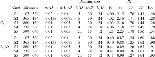
) and zero normal-pressure-gradient boundary conditions are prescribed. At the outlet boundary, the velocity is set to a zero normal gradient and the pressure is fixed at zero. At the free stream boundary, free-slip and zero normal-gradient boundary conditions are applied for the velocity and pressure, respectively. The topology of the mesh also follows that used in Shenoy & Kleinstreuer (Reference Shenoy and Kleinstreuer2008), and the computational domain is discretized with hexahedral elements; see figure 1(b). In the vicinity of the disk, the grids are finer to better resolve the steep gradient in this region. To assess the effects of the spatial and temporal resolutions on the results, three cases with different spatial and temporal resolutions are considered; see cases S1–S3 in table 1, where
 $n_{1}$
denotes the element size in the wall-normal direction near the disk surface,
 $\unicode[STIX]{x0394}t$
is the time step used in the simulations,
 $\mathit{Re}_{s}$
denotes the Reynolds number based on the free stream velocity (
 $U_{s}$
) and the disk diameter (
 $D$
) and
 $L_{w}$
denotes the recirculation length, which is defined as the streamwise distance from the centre of the disk to the position where the streamwise velocity changes sign from negative to positive. In the considered Reynolds number region (i.e.
 $\mathit{Re}_{s}<\mathit{Re}_{c1}$
), the flow is steady and axisymmetric (Auguste et al.
Reference Auguste, Fabre and Magnaudet2010). As shown in table 1, only very small variations are observed in the results for
 $C_{z}$
and
 $L_{w}$
calculated for the different spatial and temporal resolutions, i.e. for cases S1–S3. To further assess the effects of the size of the computational domain on the calculated results, two more cases are conducted with a reduced computational domain size, see cases S4 and S5 in table 1. The meshes used in cases S3–S5 are designed to be of an equivalent density. As shown in table 1, a good convergence is observed in the results of
 $C_{z}$
and
 $L_{w}$
for cases S3–S5. It is concluded that the effects of the size of the computational domain on the calculated results are negligible for case S3. Finally, the axial drag coefficient (
 $C_{z}$
) and recirculation length (
 $L_{w}$
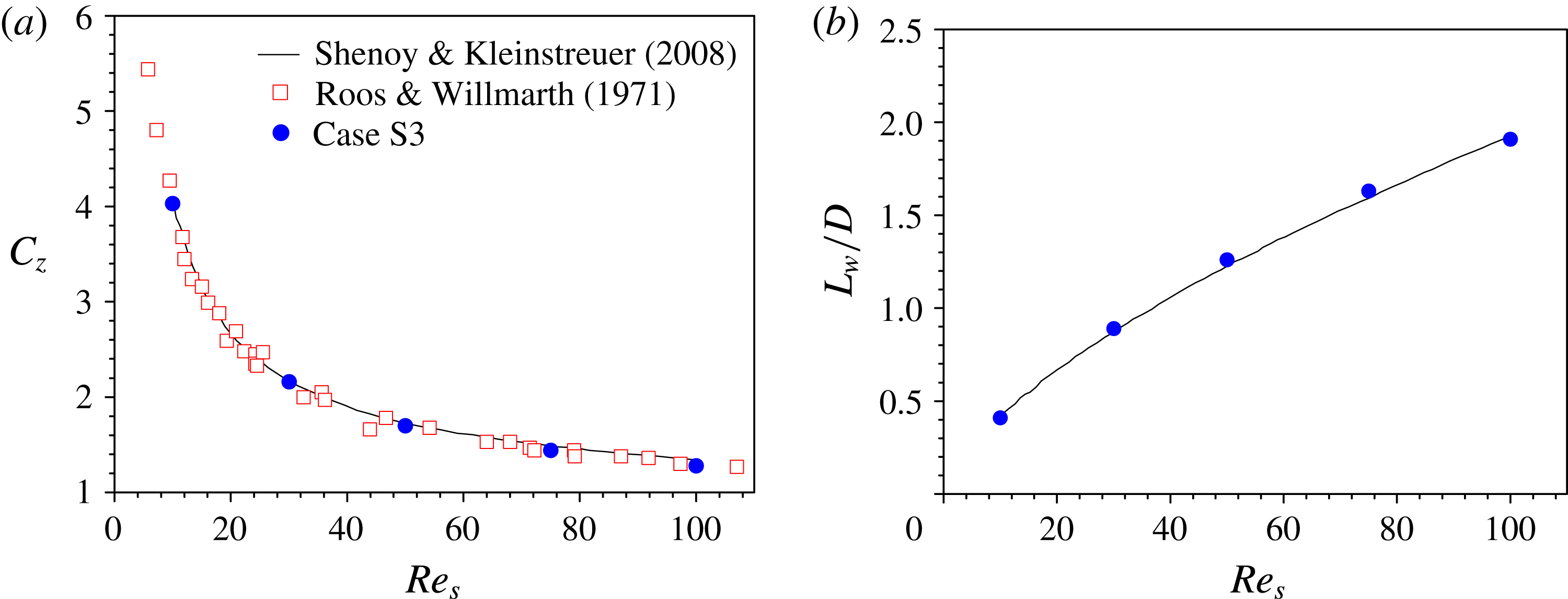
) obtained for case S3 are in good agreement with the DNS results reported by Shenoy & Kleinstreuer (Reference Shenoy and Kleinstreuer2008) and the experimental measurements reported by Roos & Willmarth (Reference Roos and Willmarth1971); see figure 2.
Stationary disk: (a) computational domain and boundary conditions (not to scale) and (b) grid structures near the disk surface.

Comparisons of the results for the steady flow normal to a circular disk: (
 $a$
) axial drag coefficient (
 $C_{z}$
) and (b) recirculation length (
 $L_{w}$
).

Results for the axial drag coefficient (
 $C_{z}$
) and the recirculation length (
 $L_{w}$
) obtained for cases of different configurations for a stationary disk. The values of
 $C_{z}$
and
 $L_{w}/D$
are shown in the last five columns.

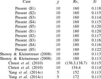
Comparisons of the Strouhal number for a stationary disk obtained in different studies.

To validate the capability of the present numerical approach for computing the unsteady wake flow, numerical simulations are conducted for Reynolds numbers of
 $\mathit{Re}_{s}=160$
and 180. As shown in table 2, the Strouhal number
 $St$
represents the wake frequency non-dimensionalized with the free stream velocity (
 $U_{s}$
) and the diameter of the disk (
 $D$
). Similar to the validation studies for the steady cases shown in table 1, the effects of the grid resolution, time step and computational domain size are also evaluated. The configurations of cases S1–S5 are kept the same as those shown in table 1. It is observed that the results of
 $St$
in the present converged case S3 agree well with the results obtained in the literature (Shenoy & Kleinstreuer Reference Shenoy and Kleinstreuer2008; Chrust et al.
Reference Chrust, Bouchet and Dušek2010; Yang et al.
Reference Yang, Wu, Zhong and Liu2014c
).
Overall, the present numerical approach yields reliable results for the flow over a circular disk. Moreover, this numerical approach has previously been successfully applied to calculate the incompressible flow around an oscillating disk (Yang, Tian & Li Reference Yang, Tian and Li2014b ).
2.3 Computational domain and boundary conditions
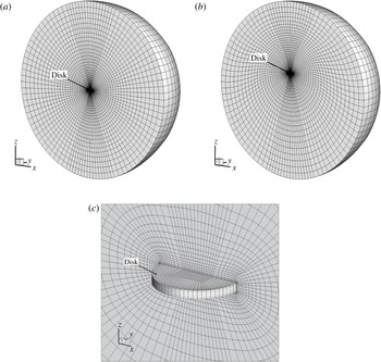
A spherical computational domain of radius
 $R_{domain}$
is used for the oscillating disk; see figure 3(a). The origin of the coordinate system is located at the centre of the computational domain, and the
 $z$
-axis coincides with the axis of the disk. The mean position of the disk is at the centre of the computational domain. On the disk surface, the no-slip boundary condition is imposed for the velocity; the pressure is set to a zero normal gradient. At the outer boundary, the velocity is set to a zero normal gradient and the pressure is fixed at zero. It has been checked carefully that the effects of the boundary condition at the outer boundary on the calculated results are negligible in the present configuration. The entire computational domain is discretized with hexahedral elements, and the grid near the disk surface is of finer resolution to resolve the steep gradient in this region; see figure 3.
The oscillatory motion of the disk is realized using the deforming mesh method, in which the topology of the mesh does not change throughout the simulation. The mesh is updated at each time step by moving the grid points based on the permanent static mesh with
 $z_{disk}=0$
, which is established at the beginning of the simulation (see figure 3
 $a$
as an example). To preserve the validity and quality of the mesh, a grid-smoothing method is applied, which is described as follows. Let
 $\boldsymbol{r}^{i}(t)$
represent the coordinates of point
 $i$
at time
 $t$
, and let
 $\boldsymbol{r}_{disk}(t)=(0,0,z_{disk})$
represent the displacement of the disk at time
 $t$
; then,
 $\boldsymbol{r}^{i}(t)$
can be determined using the following equation:
 $$\begin{eqnarray}\boldsymbol{r}^{i}(t)=\boldsymbol{r}^{i}(0)+\boldsymbol{r}_{disk}(t)f^{\ast }.\end{eqnarray}$$
The scaling function
 $f^{\ast }$
in equation (2.5) is determined by the distance of the grid point from the centre of the disk as follows:
 $$\begin{eqnarray}f^{\ast }=\left\{\begin{array}{@{}ll@{}}1 & \text{if }|\boldsymbol{r}^{i}(0)|\leqslant R_{1}\\ 0.5\sin \left[\unicode[STIX]{x03C0}\left({\displaystyle \frac{|\boldsymbol{r}^{i}(0)|-R_{2}}{R_{1}-R_{2}}}-0.5\right)\right]+0.5 & \text{if }R_{1}<|\boldsymbol{r}^{i}(0)|<R_{2}\\ 0 & \text{if }|\boldsymbol{r}^{i}(0)|\geqslant R_{2}.\end{array}\right.\end{eqnarray}$$
Here, the values of
 $R_{1}$
and
 $R_{2}$
in equation (2.6) are taken to be
 $R_{1}=2.5D$
and
 $R_{2}=R_{domain}$
, respectively, where
 $R_{domain}$
is the radius of the spherical computational domain. Using the scaling function
 $f^{\ast }$
, a smooth grid deformation can be obtained between the disk and the outer boundary. Thus, a good mesh quality can always be maintained during a simulation. Figure 3
 $(b)$
shows an example of the grid structures at the maximum amplitude considered in this study, i.e.
 $z_{disk}=3.82D$
at
 $KC=24$
.
Oscillating disk: cut-away views of the computational domain and grid structures (
 $a$
) at the mean disk position
 $z_{disk}=0$
, (b) at the maximum disk displacement (
 $z_{disk}\approx 3.82D$
at
 $KC=24$
as an example) and (
 $c$
) in a detailed zoom of the region near the disk surface.

2.4 Convergence studies
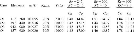
To assess the effects of the spatial and temporal resolutions on the calculated results, three cases with different numbers of grid elements and time steps, i.e. cases
 $O1$
–
 $O3$
in table 3, are considered. For each case, the results for three different flow configurations, i.e.
 $(\mathit{Re},KC)=(245,24.5)$
,
 $(600,15)$
and
 $(900,7.5)$
, are presented. The parameters
 $C_{D}$
and
 $C_{M}$
shown in table 3 are the drag and inertia coefficients, respectively, which are calculated by splitting the axial force (
 $F_{z}$
) into drag and inertial terms following the Morison equation (Morison et al.
Reference Morison, O’Brien, Johnson and Schaaf1950), which states that
 $$\begin{eqnarray}F_{z}=-C_{D}\unicode[STIX]{x1D70C}\frac{\unicode[STIX]{x03C0}}{8}D^{2}u_{z}(t)|u_{z}(t)|-C_{M}\unicode[STIX]{x1D70C}\frac{\unicode[STIX]{x03C0}}{4}t_{d}D^{2}\dot{u}_{z}(t).\end{eqnarray}$$
In this study,
 $C_{D}$
and
 $C_{M}$
were calculated using the least-squares method. As shown in table 3, for all three considered flow configurations, the results of
 $C_{D}$
and
 $C_{M}$
obtained in cases
 $O2$
and
 $O3$
agree well with each other, indicating reasonable convergence with increasing spatial and temporal resolutions. The effects of the size of the computational domain on the calculated results are evaluated by considering a larger domain of radius
 $R_{domain}=30D$
; see case
 $O4$
in table 3. Case
 $O4$
corresponds to a similar spatial resolution and the same time step in case
 $O2$
. The results for
 $C_{D}$
and
 $C_{M}$
obtained in case
 $O4$
agree well with those in cases
 $O2$
and
 $O3$
, indicating that a computational domain of radius
 $R_{domain}=20D$
is sufficient to eliminate the effects of the outer boundary on the calculated results.
Results for the drag coefficient (
 $C_{D}$
) and inertia coefficient (
 $C_{M}$
) obtained for cases of different spatial and temporal resolutions for an oscillating disk.

Axial drag coefficient (
 $C_{z}$
) with respect to the position of the disk (
 $z_{disk}$
) at (
 $a$
)
 $\mathit{Re}=245$
and
 $KC=24.5$
, (b)
 $\mathit{Re}=600$
and
 $KC=15$
and (
 $c$
)
 $\mathit{Re}=900$
and
 $KC=7.5$
.

Moreover, the time traces of
 $C_{z}$
for the three considered
 $(\mathit{Re},KC)$
configurations are plotted against
 $z_{disk}$
in figure 4. Good consistency is found among the results of cases
 $O2$
–
 $O4$
; this again demonstrates that the effects of the spatial and temporal resolutions and of the size of the computational domain on the calculated results are negligible in the present study. In the following, all reported simulations are performed using the set-up used in case
 $O2$
, i.e. with 397 440 grid elements, a time step of
 $T/10000$
and a computational domain of radius
 $20D$
.
3 Results and discussion
According to the DNS studies performed by Shenoy & Kleinstreuer (Reference Shenoy and Kleinstreuer2008) concerning the uniform flow normal to a circular disk of
 $\unicode[STIX]{x1D712}=10$
, the flow is steady and axisymmetric about the axis of the disk when
 $\mathit{Re}<135$
. As the Reynolds number increases, regular bifurcation with a loss of azimuthal symmetry occurs. Similarly, for the oscillating disk considered in the present study, non-axisymmetric bifurcation may occur as
 $\mathit{Re}$
and
 $KC$
vary. Here, the flow regimes around a circular disk of
 $\unicode[STIX]{x1D712}=10$
are investigated in the considered
 $\mathit{Re}$
–
 $KC$
space, i.e. for
 $50\leqslant \mathit{Re}\leqslant 800$
and
 $1\leqslant KC\leqslant 24$
.
The critical boundaries between different flow regimes in
 $\mathit{Re}$
–
 $KC$
space.

Numerical simulations were performed for 151 pairs of
 $\mathit{Re}$
and
 $KC$
values represented by solid dots in figure 5. Preliminary inspection on the calculated flow field indicates that there are at least three types of flow regimes in the considered
 $\mathit{Re}$
–
 $KC$
space, i.e., one axisymmetric flow region in the middle and two non-axisymmetric flow regions in the low- and high-
 $KC$
regions. It is noteworthy that the onset of non-axisymmetry is not always clear cut. The magnitude of the transverse force acting on the disk is closely related to the level of non-axisymmetry of the flow. Here, the magnitude of the transverse force coefficient is calculated as
 $C_{xy}=\sqrt{C_{x}^{2}+C_{y}^{2}}$
. Close to the threshold of the axisymmetric and non-axisymmetric regimes, any perturbation is either exponentially amplified or damped. Therefore, the accurate threshold is determined by linear interpolation of the growth rate of
 $C_{xy}$
. The details of the procedures used to determine the critical value of
 $\mathit{Re}$
and
 $KC$
corresponding to the axisymmetric and non-axisymmetric bifurcations are given in the Appendix. The two solid lines in figure 5 represent the threshold between axisymmetric and non-axisymmetric regimes. Further careful examination reveals that the non-axisymmetric flow begins to rotate around the axis of the disk as the Reynolds number increases. The boundary between the rotating and non-rotating flow regimes is identified by the dashed lines in figure 5. Finally, five flow regimes in the considered
 $\mathit{Re}$
–
 $KC$
space are revealed here: (I) axisymmetric flow (AS), (II) planar symmetric flow in the low-
 $KC$
region (PSL), (III) azimuthally rotating flow in the low-
 $KC$
region (ARL), (IV) planar symmetric flow in the high-
 $KC$
region (PSH) and (V) azimuthally rotating flow in the high-
 $KC$
region (ARH). In the following, we select one example case from each flow regime and present the corresponding force coefficients and flow visualizations.
3.1 Regime I: axisymmetric flow (AS)
Figure 6 shows the time traces of the force coefficients for the AS regime, where
 $\mathit{Re}=600$
and
 $KC=15$
. As shown, a periodic variation in
 $C_{z}$
is observed, indicating a well-developed flow. However, the transverse force coefficients
 $C_{x}$
and
 $C_{y}$
are zero.
Time traces of the force coefficients
 $C_{x}$
,
 $C_{y}$
and
 $C_{z}$
of the disk over 5 oscillation cycles in the AS regime, where
 $\mathit{Re}=600$
and
 $KC=15$
.

Figure 7 shows the three-dimensional vortical structures identified based on the
 $Q$
-criterion for
 $\mathit{Re}=600$
and
 $KC=15$
in the AS regime. As shown in figure 7, the flow is symmetric about the axis of the disk throughout the oscillation cycle. In the presented case, circular vortex rings are repeatedly generated with the periodic oscillations of the disk (see movie 1 of the online supplementary movies available at https://doi.org/10.1017/jfm.2016.800). This vortex shedding results in oscillations in the time traces of
 $C_{z}$
at higher frequencies. As mentioned previously, the critical Reynolds number for the non-axisymmetric bifurcation of the uniform flow normal to a circular disk with
 $\unicode[STIX]{x1D712}=10$
has been reported to be
 $\mathit{Re}_{c1}\approx 135$
(Shenoy & Kleinstreuer Reference Shenoy and Kleinstreuer2008) and
 $\mathit{Re}_{c1}\approx 129.6$
(Chrust et al.
Reference Chrust, Bouchet and Dušek2010). Although the Reynolds number in the case depicted in figure 7 is 600, which is significantly higher than the reported
 $\mathit{Re}_{c1}$
values, the flow in this oscillating case is still axisymmetric. One may argue that the Reynolds number defined for the oscillating case considered in this study is based on the maximum velocity of the disk [
 $U_{max}$
, see equation (1.1)], thereby resulting in a nominally higher Reynolds number. However, if we calculate an average Reynolds number based on the average magnitude of the velocity of the oscillating disk, then this average Reynolds number is
 $\mathit{Re}_{ave}=382$
, which is still significantly higher than the reported values of
 $\mathit{Re}_{c1}$
. This finding implies the existence of fundamental differences in fluid dynamics between a unidirectional flow and an oscillatory flow. Notably, the exactly circular vortical rings shown in figure 7 have not been observed in the wake of the uniform flow normal to a circular disk. This is because, for the uniform flow normal to a disk, the critical Reynolds number for the onset of vortex shedding is higher than the critical Reynolds number for non-axisymmetric bifurcation.
Vortical structures identified based on the
 $Q$
-criterion during one oscillation cycle in the AS regime, where
 $\mathit{Re}=600$
and
 $KC=15$
.

3.2 Regime II: planar symmetric flow in the low-
 $KC$
region (PSL)

Figure 8 shows the force coefficient results for the PSL regime, where
 $\mathit{Re}=411$
and
 $KC=2.57$
. As shown in figure 8(a), the values of
 $C_{x}$
and
 $C_{y}$
are comparable to the value of
 $C_{z}$
. The time traces of the force coefficients are periodic; however, the periods of
 $C_{x}$
and
 $C_{y}$
are one half of the period of
 $C_{z}$
. This finding indicates that the transverse force oscillates twice during one oscillation cycle. It is evident that the noticeable transverse force acting on the disk arises because the flow surrounding the disk is no longer axisymmetric.
Force coefficient results for the disk over 5 oscillation cycles in the PSL regime, where
 $\mathit{Re}=411$
and
 $KC=2.57$
: (
 $a$
) time traces of
 $C_{x}$
,
 $C_{y}$
and
 $C_{z}$
and (b) a phase-space plot of
 $C_{x}$
and
 $C_{y}$
.

Vortical structures identified based on the
 $Q$
-criterion during one oscillation cycle for the PSL regime, where
 $\mathit{Re}=411$
and
 $KC=2.57$
.

The vortical structures identified based on the
 $Q$
-criterion for
 $\mathit{Re}=411$
and
 $KC=2.57$
in the PSL regime are shown in figure 9. As shown in figure 9, the flow around the disk in the PSL regime appears with a planar symmetric pattern rather than with an axisymmetric pattern. As the disk oscillates, vortex shedding initially begins along one side of the disk edge, and then, a crescent-moon-shaped vortex is generated, eventually resulting in a non-axisymmetric flow. Figure 9 shows that non-axisymmetric vortex shedding occurs twice during one oscillation cycle; accordingly, the transverse force coefficients
 $C_{x}$
and
 $C_{y}$
also oscillate twice in one cycle. A more detailed animation of the vortex shedding process has been included in the online supplementary material (movie 2).
Contours of the axial vorticity (
 $\unicode[STIX]{x1D714}_{z}$
) on various
 $z$
planes for the PSL regime, where
 $\mathit{Re}=411$
,
 $KC=2.57$
and
 $z_{disk}=0$
. The circle is the projection of the disk. Positive and negative values of
 $\unicode[STIX]{x1D714}_{z}$
are represented by solid and dashed lines, respectively.

Figure 8(b) shows the phase-space plot of the
 $C_{x}$
and
 $C_{y}$
time traces shown in figure 8(a). The transverse force acting on the disk appears to oscillate back and forth along a fixed orientation, indicating that the flow is indeed planar symmetric and that the direction of the transverse force lies within the symmetry plane. The orientation of the symmetry plane is selected randomly. As shown in figure 10, the axial vorticity (
 $\unicode[STIX]{x1D714}_{z}$
) contour plots on several
 $z$
planes again demonstrate that the flow is planar symmetric. The present planar symmetric flow recalls the planar symmetric (or reflectionally symmetric) modes of the uniform flow normal to a circular disk at low Reynolds numbers, such as the SS (Fabre et al.
Reference Fabre, Auguste and Magnaudet2008), ‘standing wave’ (SW) (Meliga et al.
Reference Meliga, Chomaz and Sipp2009) and Zz (Auguste et al.
Reference Auguste, Fabre and Magnaudet2010) modes. Notably, the planar symmetric flow is one-sided with respect to the disk axis; see the flow observations in figures 9 and 10. This is because the vortex shedding locations on the two sides of the disk are always with the same orientation; see figure 9. The resulting mean value of the transverse force acting on the disk is non-zero; see figure 8(b). For the uniform flow normal to a circular disk, a non-zero mean transverse force has also been observed in the SS and Zz modes.
Because a similar planar symmetric flow regime is observed in the high-
 $KC$
region (see § 3.4), the present flow regime is referred to as the regime of planar symmetric flow in the low-
 $KC$
region (PSL).
3.3 Regime III: azimuthally rotating flow in the low-
$KC$
region (ARL)

Figure 11 shows the force coefficient results for the ARL regime, where
 $\mathit{Re}=800$
and
 $KC=2.5$
. Compared with the time traces of the force coefficients in the PSL regime (see figure 8
a), the time traces of the force coefficients in the ARL regime (see figure 11
a) are similar overall except for the slight variation in the envelopes of
 $C_{x}$
and
 $C_{y}$
. Figure 11
 $(b)$
shows the phase-space plot of
 $C_{x}$
and
 $C_{y}$
over 64 oscillation cycles. A very slow rotation is observed in the transverse force. The arrow in figure 11
 $(b)$
indicates the direction of rotation of the transverse force. It appears that the flow rotates slowly as the disk passes through successive oscillations. Figure 12 shows the evolution of the axial vorticity (
 $\unicode[STIX]{x1D714}_{z}$
) contour on the plane
 $z/D=1$
when
 $z_{disk}=0$
with a time interval of
 $13T$
. It is observed that the flow is continuously rotating about the axis of the disk.
Force coefficient results for the disk in the ARL regime, where
 $\mathit{Re}=800$
and
 $KC=2.5$
: (
 $a$
) time traces of
 $C_{x}$
,
 $C_{y}$
and
 $C_{z}$
over 5 oscillation cycles and (b) a phase-space plot of
 $C_{x}$
and
 $C_{y}$
over 64 oscillation cycles.

Evolution of the axial vorticity
 $\unicode[STIX]{x1D714}_{z}$
on the
 $z/D=1$
plane for the ARL regime, where
 $\mathit{Re}=800$
,
 $KC=2.5$
and
 $z_{disk}=0$
. The circle is the projection of the disk. Positive and negative values of
 $\unicode[STIX]{x1D714}_{z}$
are represented by solid and dashed lines, respectively.

Vortical structures identified based on the
 $Q$
-criterion during one oscillation cycle for the ARL regime, where
 $\mathit{Re}=800$
and
 $KC=2.5$
.

The vortical structures identified based on the
 $Q$
-criterion for
 $\mathit{Re}=800$
and
 $KC=2.5$
in the ARL regime are shown in figure 13 and the online supplementary material (movie 3). Although the rotational motion of the flow is very slow, the three-dimensional vortical structures in the ARL regime are more complicated than those in the PSL regime; see figure 9. For the case of the flow normal to a circular disk, the flow begins to rotate about the axis of the disk after the secondary Hopf bifurcation. The planar symmetry observed in the previous SS mode no longer holds. The flow exists in a YY state instead; see figure 5 in Shenoy & Kleinstreuer (Reference Shenoy and Kleinstreuer2008). However, the ‘Yin-Yang’ mode observed in the uniform flow normal to a circular disk is not observed in the rotating flow considered here. As shown in figure 12, the instantaneous rotating flow is approximately planar symmetric, as observed in the PSL regime; see figure 10. This implies that the planar symmetric nature of the flow in the PSL regime is inherited in the ARL regime. Therefore, similar to the flow in the PSL regime, the flow in the ARL regime is also one-sided with respect to the disk axis, and this feature is again associated with a non-zero mean transverse force (see figure 11
b).
Because a similar azimuthal rotating flow regime is observed in the high-
 $KC$
region (see § 3.5), the present flow regime is referred to as the regime of azimuthal rotating flow in the low-
 $KC$
region (ARL).
3.4 Regime IV: planar symmetric flow in the high-
$KC$
region (PSH)

Figure 14 shows the force coefficient results for the PSH regime, where
 $\mathit{Re}=500$
and
 $KC=20$
. As shown in figure 14(a), the values of
 $C_{x}$
and
 $C_{y}$
are comparable to the value of
 $C_{z}$
, indicating a non-axisymmetric flow. Similar to the PSL regime (see figure 8
 $a$
), the time traces of the force coefficients are periodic and the periods of
 $C_{x}$
and
 $C_{y}$
are one half of the period of
 $C_{z}$
. A high-frequency fluctuation is evident in
 $C_{z}$
. This is because the vortex shedding along the disk occurs more frequently in this high-
 $KC$
case than that in low-
 $KC$
cases.
Force coefficient results for the disk over 5 oscillation cycles in the PSH regime, where
 $\mathit{Re}=500$
and
 $KC=20$
: (
 $a$
) time traces of
 $C_{x}$
,
 $C_{y}$
and
 $C_{z}$
and (b) a phase-space plot of
 $C_{x}$
and
 $C_{y}$
.

Figure 14(b) shows the phase-space plot of
 $C_{x}$
and
 $C_{y}$
for
 $\mathit{Re}=500$
and
 $KC=20$
in the PSH regime. As observed in the PSL regime (see figure 8
 $b$
), the transverse force acting on the disk in the PSH regime has a fixed orientation and a non-zero mean value, indicating a one-sided planar symmetric flow. The transverse force acting on the disk oscillates within the plane of symmetry.
Vortical structures identified based on the
 $Q$
-criterion during one oscillation cycle for the PSH regime, where
 $\mathit{Re}=500$
and
 $KC=20$
.

Contours of the axial vorticity (
 $\unicode[STIX]{x1D714}_{z}$
) on various
 $z$
planes for the PSH regime, where
 $\mathit{Re}=500$
,
 $KC=20$
and
 $z_{disk}=0$
. The circle is the projection of the disk. Positive and negative values of
 $\unicode[STIX]{x1D714}_{z}$
are represented by solid and dashed lines, respectively.

The vortical structures identified based on the
 $Q$
-criterion for the case with
 $\mathit{Re}=500$
and
 $KC=20$
in the PSH regime are shown in figure 15. For the cases at high
 $KC$
, the disk travels a farther distance and the vortical structures behind the disk are more adequately developed. Therefore, apparent hairpin vortices are observed in figure 15. However, the vortices are shed in a fixed azimuthal direction with respect to the disk, unlike the double-sided vortex shedding mode observed in the ‘standing wave’ (SW) mode for the flow normal to a circular disk; see figure 8 in Shenoy & Kleinstreuer (Reference Shenoy and Kleinstreuer2008). Figure 16 shows the contours of the axial vorticity (
 $\unicode[STIX]{x1D714}_{z}$
) on various
 $z$
planes for the case of
 $\mathit{Re}=500$
,
 $KC=20$
and
 $z_{disk}=0$
. The findings again indicate that the flow is planar symmetric. A more detailed animation of the vortex shedding process has been included in the online supplementary material (movie 4). In consideration of the planar symmetric flow regime observed in the low-
 $KC$
region (the PSL regime), as presented in § 3.2, the present regime is referred to as the regime of planar symmetric flow in the high-
 $KC$
region (PSH).
3.5 Regime V: azimuthally rotating flow in the high-
$KC$
region (ARH)

Figure 17 shows the force coefficient results for the ARH regime, where
 $\mathit{Re}=600$
and
 $KC=24$
. As shown in figure 17(a),
 $C_{z}$
varies periodically, whereas
 $C_{x}$
and
 $C_{y}$
exhibit a slow variation in magnitude. The phase-space plot of
 $C_{x}$
and
 $C_{y}$
shown in figure 17(b) indicates a rotational motion of the flow. Compared with the rotational motion observed in the ARL regime (see figure 11
 $b$
), the rotational motion seen in this case is much faster. Figure 18 shows the evolution of the axial vorticity (
 $\unicode[STIX]{x1D714}_{z}$
) contours on the
 $z/D=4$
plane when
 $z_{disk}=0$
with a time interval of
 $2T$
. It is observed that the flow is continuously rotating about the axis of the disk.
Force coefficient results for the disk in the ARH regime, where
 $\mathit{Re}=600$
and
 $KC=24$
: (
 $a$
) time traces of
 $C_{x}$
,
 $C_{y}$
and
 $C_{z}$
over 5 oscillation cycles and (b) a phase-space plot of
 $C_{x}$
and
 $C_{y}$
over 12 oscillation cycles.

Evolution of the axial vorticity
 $\unicode[STIX]{x1D714}_{z}$
on the plane
 $z/D=4$
for the ARH regime, where
 $\mathit{Re}=600$
,
 $KC=24$
and
 $z_{disk}=0$
. The circle is the projection of the disk. Positive and negative values of
 $\unicode[STIX]{x1D714}_{z}$
are represented by solid and dashed lines, respectively.

Vortical structures identified based on the
 $Q$
-criterion during one oscillation cycle for the ARH regime, where
 $\mathit{Re}=600$
and
 $KC=24$
.

Figure 19 shows the variations in the vortical structures identified based on the
 $Q$
-criterion during one oscillation cycle for
 $\mathit{Re}=600$
and
 $KC=24$
in the ARH regime. The observed flow structures are more disordered than those in the PSH regime; see figure 15 and the online supplementary material (movie 5). This is because the Reynolds number in the ARH regime is higher than that in the PSH regime. Hairpin vortical structures are clearly observed in figure 19, as in the wake of the uniform flow normal to a disk. It is again observed that the vortical structures are one-sided with respect to the axis of the disk and that the mean transverse force acting on the disk is non-zero; see figure 17(b). In consideration of the azimuthal rotating flow regime observed in the low-
 $KC$
region (the ARL regime), as discussed in § 3.3, the present regime is referred to as the regime of azimuthally rotating flow in the high-
 $KC$
region (ARH).
3.6 Discussion on the steady and oscillatory flow regimes
Recalling the bifurcation scenarios in the wake of the uniform flow normal to a thin disk (see § 1), several flow regimes are revealed successively as
 $\mathit{Re}$
increases: ‘steady axisymmetric state’ (Auguste et al.
Reference Auguste, Fabre and Magnaudet2010), ‘steady asymmetric state’ Shenoy & Kleinstreuer (Reference Shenoy and Kleinstreuer2008), ‘reflectional symmetry breaking’ (Fabre et al.
Reference Fabre, Auguste and Magnaudet2008) and later some more complicated states depending on the aspect ratio of the disk. It is noted that all these states are used for describing the ‘steady- flow’ situation with a constant
 $\mathit{Re}$
. For the oscillating disk case, the ‘steady-flow’ situation is never held, instead, the actual Reynolds number increases and decreases as the disk oscillates. The saturated ‘steady-flow’ state at a particular
 $\mathit{Re}$
is not achievable in the oscillating case. Moreover, compared with the ‘steady-flow’ case, the oscillating disk moves back and forth periodically, the disk may go into its own wake. However, it does not mean that the oscillating disk case is not comparable to the ‘steady-flow’ case. A sufficiently large
 $KC$
of an oscillating disk provides a large distance for the evolution of wake flow, therefore giving us an opportunity to catch some scenario fragments which are similar to those ‘steady-flow’ states.
In this study, the range of
 $KC$
is up to 24. At the lower part of figure 5, the regimes PSL and ARL are in the range of
 $2.5<KC<7$
, approximately, corresponding to an oscillatory amplitude of
 $0.4D<a<1.4D$
. This amplitude is too small to have a developed wake flow, as confirmed in figures 9 and 13 and movies 2 and 3 in the online supplementary material. At the upper part of figure 5, the value of
 $KC$
in the regimes PSH and ARH is up to 24, corresponding to an oscillatory amplitude of
 $a\approx 3.82D$
. This distance allows a wake evolution as that in the ‘steady-flow’ case. As shown in the case of
 $\mathit{Re}=500$
and
 $KC=20$
(see figure 15), the flow is planar symmetric as described in § 3.4. At the topmost and lowest locations (see the pictures at
 $t=2T/8$
and
 $6T/8$
respectively in figure 15), the actual instantaneous Reynolds number is very small. Therefore, the toroidal vortex is generated approximately. This could be interpreted as a co-existence of different ‘steady-flow’ states in the oscillating disk case, see also movie 4 in the online supplementary material. For the case of
 $Re=600$
and
 $KC=24$
(see figure 19), the increase in Reynolds number results in a new regime corresponding to the ‘reflectional symmetry breaking state’ in the ‘steady-flow’ case (Fabre et al.
Reference Fabre, Auguste and Magnaudet2008).
It appears that there are some connections between the oscillating disk at a large
 $KC$
and the ‘steady-flow’ case. However, it must be kept in mind that the oscillating disk case presented here are intrinsically different with the ‘steady-flow’ situation. In other words, the
 $KC=24$
is still too small to be considered as a ‘sufficiently large’
 $KC$
at which those bifurcations in the ‘steady-flow’ case could be observed in one oscillating cycle.
4 Concluding remarks
The flow around an oscillating circular disk was investigated using the DNS approach. The disk was forced to oscillate sinusoidally along its axis. The aspect ratio (diameter/thickness) of the disk was 10. The ranges considered for the Reynolds number (
 $\mathit{Re}$
) and the Keulegan–Carpenter number (
 $KC$
) were
 $50\leqslant \mathit{Re}\leqslant 800$
and
 $1\leqslant KC\leqslant 24$
, respectively. In the considered
 $\mathit{Re}$
–
 $KC$
space, one axisymmetric flow regime and two non-axisymmetric flow regimes were identified. In each non-axisymmetric flow regime, the flow was planar symmetric at lower Reynolds numbers and began to rotate about the axis of the disk as the Reynolds number increased. Therefore, five flow regimes were identified: (I) axisymmetric flow (AS), (II) planar symmetric flow in the low-
 $KC$
region (PSL), (III) azimuthally rotating flow in the low-
 $KC$
region (ARL), (IV) planar symmetric flow in the high-
 $KC$
region (PSH) and (V) azimuthally rotating flow in the high-
 $KC$
region (ARH). In the non-axisymmetric flow regimes, the flow around the disk was found to be one-sided with respect to the axis of the disk and associated with a non-zero mean value of the transverse force acting on the disk.
It should be noted that the critical boundaries between the different flow regimes in the
 $\mathit{Re}$
–
 $KC$
space were determined based on a limited number of numerical simulations. More accurate boundaries could be obtained through more extensive numerical simulations. Because only one disk aspect ratio, namely,
 $\unicode[STIX]{x1D712}=10$
, was considered in this study, further research is planned to study the effects of the aspect ratio on the flow regimes and the critical boundaries between different flow regimes.
Acknowledgements
The authors would like to thank the support from Shanghai Yang Fan Program (grant no. 15YF1406100), the National Natural Science Foundation of China (grant nos 51509152, 11632011 and 51239007) and the Newton Research Collaboration Programme (grant no. NRCP/1415/211). The numerical simulations were supported by Center for HPC, Shanghai Jiao Tong University. The authors acknowledge the constructive comments of the reviewers which indeed improved the quality of this paper.
Supplementary movies
Supplementary movies are available at https://doi.org/10.1017/jfm.2016.800.
Appendix
This appendix provides additional information of the procedures used to determine the accurate critical
 $\mathit{Re}$
and
 $KC$
numbers for the axisymmetric and non-axisymmetric bifurcations. The threshold is determined roughly based on the extensive simulations at various
 $\mathit{Re}$
and
 $KC$
as indicated by the solid dots in figure 5. It is observed that the threshold lays between the axisymmetric case
 $(\mathit{Re},KC)=(300,2.5)$
and the non-axisymmetric case
 $(\mathit{Re},KC)=(300,3)$
. Now we use a slightly perturbed flow as the initial condition for the case
 $(\mathit{Re},KC)=(300,3)$
. As shown in figure 20(a), a growth of the amplitude of the transverse force coefficient
 $C_{xy}$
is observed. By fitting the envelope of the time traces of
 $C_{xy}$
to an exponential function of time, a growth rate of 2.2542 (see figure 20
 $c$
) is determined (Ghidersa & Dus̆ek Reference Ghidersa and Dus̆ek2000; Bohorquez et al.
Reference Bohorquez, Sanmiguel-rojas, Sevilia, Jiménez-gonzález and Martínez-bazán2011). Similarly, the case of
 $(\mathit{Re},KC)=(300,2.5)$
is conducted with the solution for the case of
 $(\mathit{Re},KC)=(300,3)$
as an initial condition. Then, a decay of the amplitude of
 $C_{xy}$
is observed and the decay rate is determined to be
 $-0.0330$
(see figure 20
b,d). By linear interpolation of the amplification rates, the threshold is obtained at
 $(\mathit{Re},KC)=(300,2.56)$
. Similar procedures are used to determine to the accurate threshold at other locations. In this study, 22 sets of simulations are performed and the determined critical
 $\mathit{Re}$
and
 $KC$
numbers are shown in table 4.
Determination of the growth/decay rates of the amplitude of
 $C_{xy}$
for the cases based on a perturbed initial condition. The time traces of
 $C_{xy}$
for the cases of (
 $a$
)
 $(\mathit{Re},KC)=(300,3)$
and (b)
 $(\mathit{Re},KC)=(300,2.5)$
, (
 $c$
) and (
 $d$
) the corresponding exponential fit of the envelop of
 $C_{xy}$
.

Critical
 $\mathit{Re}$
and
 $KC$
numbers for the axisymmetric and non-axisymmetric bifurcations.