1. Introduction
When a shock wave interacts with a perturbed interface separating two fluids of different density, baroclinic vorticity is deposited at the interface due to the misalignment of the pressure gradient at the shock wave with the density gradient at the interface, which in turn drives the interface perturbation growth through distinct phases: initial startup (Lombardini & Pullin Reference Lombardini and Pullin2009; Li et al. Reference Li, Chen, Zhi and Luo2024); linear growth (Richtmyer Reference Richtmyer1960; Meyer & Blewett Reference Meyer and Blewett1972; Yang et al. Reference Yang, Zhang and Sharp1994; Wouchuk Reference Wouchuk2001); nonlinear growth (Mikaelian Reference Mikaelian2003; Dimonte & Ramaprabhu Reference Dimonte and Ramaprabhu2010; Zhang et al. Reference Zhang, Deng and Guo2018); ultimate turbulent mixing (Noble et al. Reference Noble, Ames, McConnell, Oakley, Rothamer and Bonazza2023; Ferguson & Jacobs Reference Ferguson and Jacobs2024). This type of hydrodynamic instability is referred to as a Richtmyer–Meshkov instability (RMI), since it was first theoretically analysed by Richtmyer (Reference Richtmyer1960) and later confirmed experimentally by Meshkov (Reference Meshkov1969). The RMI is widely present in practical applications such as scramjet engines (Urzay Reference Urzay2018; Wu et al. Reference Wu, Li, Lu, Xu and liang2024; Bajaj et al. Reference Bajaj, Kansara, Nath, Vashishtha and Sahoo2025), where shock–interface interactions rapidly destabilize fuel–oxidizer layers, thereby promoting mixing and accelerating combustion. As noted by Huete et al. (Reference Huete, Sánchez, Williams and Urzay2015), RMI provides an effective mechanism for enhancing fuel–oxidizer mixing and facilitating faster combustion. In contrast, in inertial confinement fusion, RMI strongly influences fuel capsule compression by disrupting its symmetry, thereby degrading net energy gain and potentially leading to ignition failure (Lindl et al. Reference Lindl, McCrory and Campbell1992; Roycroft et al. Reference Roycroft, Sauppe and Bradley2022).
In terms of the interplay between interface dynamics and chemical reaction, RMI can be classified into two fundamental types: inert RMI, in which the material composition remains unchanged and interface evolution is governed purely by hydrodynamics; and reactive RMI, in which chemical reactions actively influence interface evolution. Extensive research on inert RMI has been conducted through theoretical (Zhang & Sohn Reference Zhang and Sohn1997; Wouchuk Reference Wouchuk2001; Mikaelian Reference Mikaelian2005; Dimonte & Ramaprabhu Reference Dimonte and Ramaprabhu2010; Zhang et al. Reference Zhang, Deng and Guo2018), experimental (Sadot et al. Reference Sadot, Erez, Alon, Oron, Levin, Erez, Ben-Dor and Shvarts1998; Jacobs & Krivets Reference Jacobs and Krivets2005; Balakumar et al. Reference Balakumar, Orlicz, Tomkins and Prestridge2008; Morgan et al. Reference Morgan, Aure, Stockero, Greenough, Cabot, Likhachev and Jacobs2012; Mohaghar et al. Reference Mohaghar, Carter, Pathikonda and Ranjan2019; Mansoor et al. Reference Mansoor, Dalton, Martínez, Desjardins, Charonko and Prestridge2020) and numerical (Latini et al. Reference Latini, Schilling and Don2007; Groom & Thornber Reference Groom and Thornber2023; Zhou et al. 2023, Reference Zhou, Ding, Cheng and Luo2024; Xie et al. Reference Xie, Luo, Zhao, Zhang and Wang2025) approaches, with comprehensive reviews synthesizing these findings (Zabusky Reference Zabusky1999; Brouillette Reference Brouillette2002; Ranjan et al. Reference Ranjan, Oakley and Bonazza2011; Zhou Reference Zhou2017a , Reference Zhoub ; Zhou et al. Reference Zhou, Sadler and Hurricane2025). By contrast, reactive RMI has received considerably less attention, despite its broader relevance to combustion and propulsion systems. This instability, involving complex interactions between hydrodynamic mechanisms and chemical kinetics, poses significant challenges for theoretical modelling, experimental diagnostics and high-fidelity numerical simulations (Yang & Radulescu Reference Yang and Radulescu2021; Bambauer et al. Reference Bambauer, Hasslberger and Ozel-Erol2023; Napieralski et al. Reference Napieralski, Cobos, Sánchez-Sanz and Huete2024).
A representative manifestation of reactive RMI is the shock–flame interaction, where a laminar flame front separates dense unburned reactants from light combustion products, forming a pronounced density contrast. Shock–flame interaction is essentially governed by two competing effects. First, baroclinic torque deforms the flame front, and shock-induced compression elevates local reactant density, pressure and temperature, jointly enhancing the overall reaction rate. Under sufficiently strong shock conditions, RMI can significantly contribute to flame acceleration, transition to turbulence and ultimately deflagration-to-detonation transition (Khokhlov et al. Reference Khokhlov, Oran and Thomas1999b ; Thomas et al. Reference Thomas, Bambrey and Brown2001; Bambauer et al. Reference Bambauer, Hasslberger and Ozel-Erol2023). Second, experiments (Thomas et al. Reference Thomas, Bambrey and Brown2001) and numerical simulations (Zhu et al. Reference Zhu, Gao, Luo, Pan, Pan and Zhang2019) have shown that chemical reaction itself can reduce flame wrinkling due to reactive burnout of the developing structures. Understanding shock–flame interactions is therefore crucial not only for elucidating the fundamental mechanisms of reactive RMI but also for addressing practical challenges in combustion instability control (Lindl et al. Reference Lindl, Landen, Edwards, Moses and Team2014; Roycroft et al. Reference Roycroft, Sauppe and Bradley2022) and shock-assisted propulsion (Huete et al. Reference Huete, Sánchez, Williams and Urzay2015; Urzay Reference Urzay2018).
Over the past decades, numerous theoretical models have been developed to describe perturbation growth in both the linear and nonlinear regimes for inert RMI (Richtmyer Reference Richtmyer1960; Sohn Reference Sohn2003; Mikaelian Reference Mikaelian2005; Zhang & Guo Reference Zhang and Guo2016). These models establish the hydrodynamic foundation for understanding shock–interface interaction. For shock–flame interaction, however, the flame front itself may be subject to intrinsic hydrodynamic instabilities. For instance, premixed flames are known to exhibit the Darrieus–Landau (DL) instability. Liberman et al. (Reference Liberman, Bychkov and Golberg1994) performed a rigorous theoretical analysis of the hydrodynamic stability of planar premixed flames by accounting for finite reaction-zone thickness and thermal–diffusive effects, and derived the classical DL growth rate from the complete reactive–diffusive formulation in the long-wavelength limit. Subsequently, Bychkov & Liberman (Reference Bychkov and Liberman2000) presented a comprehensive review of premixed flame dynamics, covering both linear and nonlinear DL instability, curved flame propagation and flame interactions with gravity, acoustic disturbances and weak shocks. These theoretical developments provide the framework for interpreting shock–flame interaction and, in particular, for distinguishing intrinsic flame instabilities from impulsively driven RMI.
Owing to rapid advances in numerical algorithms (Chen & Deng Reference Chen and Deng2024) and high-performance parallel computing, numerical simulations have become a primary tool for investigating shock–flame interactions (Attal & Ramaprabhu Reference Attal and Ramaprabhu2015; Diegelmann et al. Reference Diegelmann, Hickel and Adams2016; Jiang et al. Reference Jiang, Dong and Chen2017; Zhu et al. Reference Zhu, Gao, Luo, Pan, Pan and Zhang2019; Fan et al. Reference Fan, Hao, Guan, Wen and Shi2022; Gong et al. Reference Gong, Zhao, Chen, Li, Zhou and Qiu2023). The seminal numerical work of Batley et al. (Reference Batley, McIntosh, Brindley and Falle1994) on the interaction of planar shocks with cylindrical flames revealed that baroclinically generated vorticity causes the flame to roll up and split. Their study further isolated the roles of chemistry and diffusion, showing the initial deformation is governed by inviscid dynamics, while subsequent evolution is significantly influenced by reactive and diffusive processes. Later, Khokhlov et al. (Reference Khokhlov, Oran and Thomas1999 b) demonstrated through high-resolution simulations that a single shock–flame interaction can enhance the energy release rate by up to a factor of 20–30, primarily driven by flame surface area increase from RMI. Simulations of a sinusoidally perturbed flame subjected to successive shocks by Jiang et al. (Reference Jiang, Dong, Chen and Li2016) showed that the evolution of reactive RMI is governed by the competition between hydrodynamic and chemical time scales, with RMI dominating the early interface dynamics and chemical reactions controlling the later stages. Numerical simulations of planar shock–spherical flame interactions by Zhu et al. (Reference Zhu, Gao, Luo, Pan, Pan and Zhang2019) showed that initial reactive-mixture gradients play a critical role in controlling flame evolution, detonation onset and vorticity generation. Recently, three-dimensional (3-D) simulations of successive shock–flame interactions by Wang & Dong (Reference Wang and Dong2022) revealed multiscale RMI-induced vortical structures and their coupling with chemical reactions, establishing clear links between flow topology and combustion dynamics. More recently, Fan et al. (Reference Fan, Wang and Zhang2025) numerically investigated shock–flame interactions in dimethyl ether–air mixtures, showing that shock strength and initial flame state critically control the evolution and transition of cool, warm and hot flames. These studies indicate that the mechanisms of shock–flame interactions are intrinsically complex and highly sensitive to initial conditions, such as shock strength and fuel composition, leading to markedly different evolutionary behaviours under seemingly similar configurations.
Compared with numerical simulations, experimental investigations of shock–flame interactions are relatively scarce, as they face significant challenges, including difficulties in generating flames with well-defined geometries (Yang & Radulescu Reference Yang and Radulescu2021), maintaining flame stability (La Flèche et al. Reference La Flèche, Xiao, Wang and Radulescu2017), limitations of ignition techniques (Lackner et al. Reference Lackner, Charareh, Winter, Iskra, Rüdisser, Neger, Kopecek and Wintner2004) and constraints in diagnostic capabilities (Meyer et al. Reference Meyer, Roy, Belovich, Corporan and Gord2005). Markstein (Reference Markstein1957) conducted a pioneering experimental study on the interaction of a finger-shaped flame with a planar shock and its reflected wave, observing pronounced Taylor-like instabilities that lead to flame inversion, acceleration and significantly enhanced burning rates. Thomas et al. (Reference Thomas, Bambrey and Brown2001) investigated laminar spherical flames impacted by incident and reflected shocks, observing a striking coupled wave in which the shock front and perturbed flame propagate together. This wave was found to propagate faster than the laminar flame speed yet remains well below the Chapman–Jouguet detonation velocity, being driven not by classical turbulence but by a chemical–acoustic feedback mechanism. La Flèche et al. (Reference La Flèche, Xiao, Wang and Radulescu2017) investigated the head-on interaction of a shock wave with a cellular flame using two novel Hele-Shaw cell configurations. It was found that shock passage induces RMI on flame cusps, leading to flame deformation, cusp inversion, enhanced small-scale mixing and potential acceleration of the burning rate. Recently, Yang & Radulescu (Reference Yang and Radulescu2021) extended the work of La Flèche et al. (Reference La Flèche, Xiao, Wang and Radulescu2017) by investigating the deformation of cellular flames following a head-on shock interaction, showing that the flame front initially behaves as an inert interface at times much shorter than the characteristic burning time, while at times comparable to the laminar flame time, chemical energy release enhances the growth of flame perturbations.
Previous experiments have primarily focused on shock interactions with spherical, finger-like and cellular flames. In practice, however, flame fronts can develop a wide range of morphologies due to hydrodynamic instabilities such as the DL and Rayleigh–Taylor instabilities (RTI), as well as thermodiffusive instability (Sivashinsky Reference Sivashinsky1983; Yang & Radulescu Reference Yang and Radulescu2021). Among these, the cylindrical bubble flame constitutes a canonical configuration whose dynamics remain largely unexplored, despite its fundamental relevance to shock–flame interactions. Studying shock interactions with cylindrical flames is especially important for several reasons. First, previous experiments of 3-D spherical flames have typically relied on schlieren diagnostics, which integrate along the line of sight and cannot fully resolve 3-D flame structures, whereas two-dimensional (2-D) configurations provide clearer interfacial dynamics suitable for detailed mechanistic analysis. Second, from a practical standpoint, many engineering applications, such as narrow-slot combustion chambers (Yakush et al. Reference Yakush, Rashkovskiy, Alexeev and Semenov2025), feature confined geometries with large cross-sectional areas but limited heights, where quasi-2-D cylindrical flames naturally arise (La Flèche et al. Reference La Flèche, Xiao, Wang and Radulescu2017). Third, as a canonical configuration in inert RMI, cylindrical bubbles subjected to shock waves have been extensively studied, offering abundant experimental data for direct comparison (Haas & Sturtevant Reference Haas and Sturtevant1987; Jacobs Reference Jacobs1992; Ranjan et al. Reference Ranjan, Oakley and Bonazza2011; Ding et al. Reference Ding, Si, Chen, Zhai, Lu and Luo2017, Reference Ding, Liang, Chen, Zhai, Si and Luo2018). This provides a unique opportunity to quantify the effects of combustion by directly comparing reactive and inert cases under similar conditions. These considerations collectively motivate the present study.
In this work, we investigate the evolution of cylindrical flames subjected to successive incident and reflected shocks using combined experimental and numerical approaches. Experimentally, a chemically reactive shock tube is newly developed to generate cylindrical hydrogen–oxygen flames with controllable radii. The evolution of flame morphology, length, width and area under varying shock Mach numbers and initial flame radii is quantified, providing rare experimental data on shock–flame interactions. Marked differences are observed between the evolution of cylindrical flames and that of inert gas cylinders. High-fidelity numerical simulations with initial conditions identical to the experiments are performed to elucidate the mechanisms governing shock–flame interactions. By comparing reactive cases with inert RMI cases (obtained by deactivating the chemical reaction source term), the relative role of chemical reactions in flame interface evolution is characterized. The vorticity distribution and its evolution in both reactive and inert configurations are further analysed to reveal the distinct dynamics of reactive and inert configurations. In addition, a numerical experiment involving two parallel, unperturbed flames separated by one cylindrical flame diameter is conducted to isolate the effect of RMI on combustion. By comparing shock–cylindrical-flame interactions with shock–unperturbed-flame interactions, the influence of RMI on combustion enhancement is quantified. Finally, the ratio of characteristic flow to chemical time scales is evaluated to assess the competition between RMI and combustion throughout the shock–flame interaction process.
2. Experimental methods
2.1. Design of a chemically reactive shock tube
The experiments are conducted in a chemically reactive shock tube newly designed at the Shock Wave Laboratory, University of Science and Technology of China. The facility consists of five sections with uniform cross-sectional area: a 2000-mm-long driver section, a 1000-mm-long driven section, a 1000-mm-long transformation section, a 2000-mm-long stabilization section and a 660-mm-long test section, as shown in figure 1(a). The lengths of these sections are determined based on the
 $x$
–
 $t$
diagrams shown in figure 2, calculated using one-dimensional (1-D) gas-dynamics theory, ensuring that the upstream rarefaction waves do not enter the test section during the period of interest. The test section has a cross-sectional area of 120 mm
 $\times$
8 mm. The small inner height (8 mm) of the test section is designed to minimize 3-D effects on the formation and evolution of cylindrical flames. To withstand the high temperature and pressure resulting from complete combustion of the reactive gas, the test section is specially designed to be made of a high-temperature resistant material. In addition, the observation windows are made of specially customized tempered optical glass.
(a) Schematics of the chemically reactive shock tube, (b) the high-speed schlieren system and (c) the gas filling apparatus.

An
 $x$
–
 $t$
diagram illustrating the shock formation and propagation with a Mach number of 1.5.

Shock waves are generated by increasing the pressure in the driver section until the diaphragm between the driver and driven sections bursts. By testing different diaphragm materials (0.5 mm polyethylene terephthalate (PET) film and 1.0 mm aluminium film) and driving gases (N
 $_2$
and He), stable incident shock waves with Mach numbers ranging from 1.1 to 1.6 can be obtained, enabling a parametric study on the effect of Mach number. Prior to each experimental run, the shock tube is filled with different gases in its respective sections: helium in the driver section, air in the driven, transformation and stabilization sections, and an argon-diluted hydrogen–oxygen mixture in the test section. Figure 1(c) illustrates the gas-filling apparatus, which consists of an acrylic guiding box. Ignition electrodes and lead wires are mounted at the top and bottom of the box, while gas inlet and outlet ports are set on the sidewalls to allow flushing with the hydrogen–oxygen–argon mixture and purging of air. Once assembled, the box is inserted into the test section. To minimize interference in the test section, the ignition electrodes and wiring are integrated into the 8-mm-thick acrylic plate. As illustrated in figure 1(c), grooves that match the size and shape of the nail-shaped electrodes are machined on the top and bottom surfaces of the plate. High-temperature adhesive is applied to the groove surfaces before inserting the electrodes, ensuring a proper gas seal once they are in place. After installation, each electrode forms a conical tip with a base radius and height of 0.4 mm, i.e. extending only 0.4 mm into the test section. This configuration enables the formation of a stable electric arc during ignition while minimizing intrusion into the flow field.
After the guiding box is inserted into the test section, a plastic film is attached to its openings to isolate the gases during filling. A supply tube is introduced through the filling port and extended to the bottom of the test section, while an oxygen sensor is installed at the venting port. The H
 $_2$
–O
 $_2$
–Ar mixture is introduced into the test section through the supply tube while air is simultaneously vented through the venting port. Once the oxygen concentration measured by the sensor reaches a stable value, the filling process is terminated. The supply tube is then removed, and the openings are sealed prior to experiments. As the shock wave reaches the end of the stabilization section, a pressure sensor generates an electrical signal that simultaneously triggers the high-speed camera and the electrode ignition system, ensuring that recording and ignition occur before shock arrival. The electrode-ignited cylindrical flame subsequently interacts first with the incident shock and then with its reflected shock. The ignition system incorporates an adjustable trigger delay, allowing control of the ignition timing and thus the flame radius at the instant of shock arrival. The flow field is recorded using a Z-type folded schlieren system coupled with a high-speed camera (FASTCAM SA5, Photron Limited), operating at 50 000 frames per second with a shutter time of 1
 $\unicode {x03BC}$
s, as shown in figure 1(b).
Image postprocessing procedure: (a) original raw schlieren image; (b) image after removal of stationary dark spots and uniform brightness/contrast adjustment; (c) extracted flame region using MATLAB, with definitions of flame length (
 $L$
), width (
 $W$
) and area (
 $S$
).

2.2. Image processing and experimental repeatability
To ensure data reliability, both the image-processing procedure and experimental repeatability are carefully evaluated. The procedure developed to extract the flame profile from schlieren images enables quantitative characterization of the flame surface in terms of length, width and area. Figure 3(a) presents the original raw experimental images without any postprocessing. It should be noted that the dark spots observed in the images are not combustion residues, as they remain at fixed spatial locations throughout the entire image sequence, despite repeated cleaning of the acrylic plate after each experiment. These spots are likely caused by localized transmittance variations of the acrylic surface induced by high-temperature exposure. Such optical artefacts neither participate in the reaction nor influence the flow field, and they can be reliably identified and excluded through comparison of consecutive frames. After removing these stationary dark spots, only uniform brightness and contrast adjustments are applied prior to interface extraction, as shown in figure 3(b). Although the above processing removes minor, small-scale density variations within the cylindrical flame, it does not compromise the accurate identification of the flame morphology. The entire flame region is then extracted using a MATLAB-based image-processing procedure. As illustrated in figure 3(c), the combustion region is divided into two parts: the red region represents the flame front and intensely reacting turbulent-like flame zones, while the blue region corresponds to the burned gas region with a relatively low reaction rate, where most of the hydrogen has already been consumed. Owing to differences in density gradients, these two regions appear grey–black and white, respectively, in the schlieren images.
For quantitative analysis, the maximum length and maximum width of the red and blue regions are measured separately and denoted as
 $L_1$
,
 $L_2$
and
 $W_1$
,
 $W_2$
, respectively. The flame length
 $L$
and width
 $W$
are defined as the arithmetic means of the corresponding values:
 $L = (({L_1 + L_2})/{2})$
,
 $W = (( {W_1 + W_2})/{2})$
. The associated uncertainties (error bars) are estimated as half of their differences:
 $\Delta L = (({|L_1 - L_2|})/{2})$
,
 $\Delta W = (({|W_1 - W_2|})/{2})$
. For the area calculation, the total flame area
 $S$
is defined as the area of the blue region (
 $S_2$
) plus one-half of the red region area (
 $S_1$
):
 $S = S_2 + ({1}/{2}) S_1$
, and the corresponding uncertainty is conservatively taken as
 $\Delta S = ({1}/{2}) S_1$
. To quantify the influence of image processing on the extracted flame area, additional sensitivity analyses have been performed. When the binarization threshold used in MATLAB for interface extraction varies within
 $\pm 5\,\%$
of the selected optimal value, the resulting variation in total flame area remains below approximately
 $3\,\%$
. Furthermore, the removed stationary spots occupy only a very small pixel fraction and do not significantly overlap with the flame boundary. A comparison of area calculations before and after spot masking shows deviations smaller than
 $1\,\%$
, indicating that spot removal does not fundamentally alter the extracted flame area. For the post-reshock turbulent-like dark regions, only global brightness and contrast scaling is applied. Repeated extractions under independently adjusted global parameters yield area variations within approximately
 $3$
%–
 $4\,\%$
, demonstrating acceptable repeatability. Considering threshold sensitivity, artefact masking influence and extraction repeatability together in a conservative manner, the overall uncertainty in flame area attributable to image processing is estimated to be within
 $\pm 5\,\%$
.
Pressure histories measured by two piezoelectric sensors.

To assess the quality and repeatability of the postshock flow, pressures are measured at the stabilization section using piezoelectric sensors. Figure 4 shows the pressure histories at two positions just upstream of the test section. Following shock passage, the pressure exhibits a stable plateau, with no noticeable attenuation or spurious oscillations. This confirms that the shock tube generates a uniform, disturbance-free postshock pressure field. To quantify the experimental repeatability, two runs with nominally identical conditions, specifically, similar shock Mach numbers and initial flame radii (listed in table 1), are performed and compared. Figure 5 presents the temporal evolution of flame length
 $L$
, width
 $W$
and area
 $S$
for these repeated runs. The close collapse of all curves demonstrates both the high repeatability of the experiments and the low uncertainty of the data-extraction procedure.
Two experimental runs with nominally identical conditions for repeatability verification. Here
 $X$
denotes the mole fraction of the corresponding gas,
 ${\textit{Ma}}$
represents the Mach number of the incident shock and
 $R$
represents the initial flame radius at the time when the incident shock arrives at the flame front.

Table 1. Long description
A table comparing two experimental runs with nominally identical conditions for repeatability verification. The table has two rows and six columns. The columns are labeled Case, Ma, X_H2, X_O2, X_Ar, and R (cm). The row labels are Run 1 and Run 2. Row 1: Run 1, 1.30, 0.16, 0.16, 0.68, 1.41. Row 2: Run 2, 1.30, 0.16, 0.16, 0.68, 1.34. The table lists the mole fractions of hydrogen (X_H2), oxygen (X_O2), and argon (X_Ar), the Mach number of the incident shock (Ma), and the initial flame radius (R) at the time when the incident shock arrives at the flame front.
Initial conditions for cases 1–3 with different shock Mach numbers. The symbols are the same as those in table 1.

Table 2. Long description
A table with three rows and five columns comparing initial conditions for different shock Mach numbers. The columns are labeled Case, Ma, X_H2, X_O2, X_Ar, and R (cm). Row 1: Case 1, Ma 1.18, X_H2 0.16, X_O2 0.16, X_Ar 0.68, R 1.30. Row 2: Case 2, Ma 1.30, X_H2 0.16, X_O2 0.16, X_Ar 0.68, R 1.30. Row 3: Case 3, Ma 1.42, X_H2 0.16, X_O2 0.16, X_Ar 0.68, R 1.30.
Temporal variations of (a) flame length
 $L$
and width
 $W$
, and (b) area
 $S$
for two repeated runs.

Schlieren images illustrating shock–flame interactions under different shock Mach numbers. Here IS, incident shock; RS, reflected shock; TS, transmitted shock; TS
 $_2$
, second transmitted shock.

3. Experimental results and discussions
This section experimentally investigates the evolution of cylindrical flames impacted successively by incident and reflected shocks. The effects of Mach number and flame radius on the overall morphological development of the flame are examined.
3.1. Shock–flame interaction under various shock strengths
Cases 1–3, featuring different shock Mach numbers, are first examined, with their initial conditions listed in table 2. All other parameters, including the flame radius immediately before shock impact and the composition of the gas mixture, are kept approximately constant across these cases. Representative schlieren images illustrating the evolution and propagation of both flame and wave structures for cases 1–3 are displayed in figure 6. At the beginning, the flame presents a nearly circular front, with the burnt gases occupying the interior region. Note that the gas inside is not fully homogeneous, as a small fraction of hydrogen remains and reacts at a rate much lower than that at the flame front. Additionally, the arc-discharge ignition generates a high-temperature kernel at the flame centre, causing the mixture near the local ignition region to burn earlier. By adjusting the electrode ignition delay time, the flame radius at
 $t=0$
(defined as the moment when the incident shock interacts with the flame front) is maintained approximately consistent across runs with different shock strengths. The initial flame interface in figure 6 is smooth and presents no visible stratification, indicating that the DL instability (Sivashinsky Reference Sivashinsky1983) exerts a negligible influence on the early-stage flame evolution under the present experimental conditions. These results demonstrate the feasibility of the present ignition technique for generating cylindrical flames.
Case 1 with
 ${\textit{Ma}}=$
1.18 is taken as an example to detail the evolution process. Prior to the arrival of the incident shock, the overall flame shape remains nearly unchanged, exhibiting only slight increases in length, width and area owing to its low propagation velocity relative to the shock wave. In contrast, the flame undergoes rapid deformation immediately after shock impact, indicating that the shock-induced deformation time scale is much shorter than the flame self-propagation time scale. At
 $t= 20\,\unicode {x03BC}\text{s}$
, the incident shock first impinges upon the upstream flame interface, compressing it into a flattened structure that subsequently undergoes phase inversion (i.e. develops with an opposite perturbation phase). As a consequence, the flame length decreases rapidly at the early stage. Note this interaction not only accelerates the upstream interface downstream but also generates a transmitted shock that propagates through the burnt region. Once the transmitted shock reaches the downstream interface, the flame is no longer compressed, and its length begins to increase rapidly owing to RMI-driven deformation of flame interface. The observed decrease in flame area at early times is likewise attributed to shock-induced compression, which continues until the transmitted shock exits the flame. After the transmitted shock passes through the downstream flame, a second curved transmitted shock emerges, which subsequently reflects off the end wall of the test section to form a reflected shock (
 $t=320\,\unicode {x03BC}\text{s}$
). At this stage, the upstream flame interface has developed into a slender spike, with its tip already reaching the downstream interface. Compared with the light-cylinder evolution in inert RMI at similar density ratios (Haas & Sturtevant Reference Haas and Sturtevant1987; Jacobs Reference Jacobs1992; Ding et al. Reference Ding, Si, Chen, Zhai, Lu and Luo2017), the spike here is noticeably sharper, and the overall flame area is larger. This phenomenon is consistently observed in numerical simulations and analysed in detail through vortex dynamics in § 4. At
 $420\,\unicode {x03BC}\text{s}$
, the reflected shock reimpacts the evolving flame, generating additional baroclinic vorticity that leads to pronounced flame deformation. In particular, turbulent-like structures develop at localized regions on the upstream and downstream interfaces, increasing flame thickness, three-dimensionality and propagation speed (
 $520\,\unicode {x03BC}\text{s}$
). Generally, the 2-D nature of the flame in the present experiments enables clearer identification of finescale structures (e.g. the formation of slender spikes) compared with previous 3-D spherical flame experiments (Thomas et al. Reference Thomas, Bambrey and Brown2001).
Temporal evolutions of (a) flame length
 $L$
, (c) width
 $W$
and (e) flame area
 $S$
under three different incident Mach numbers. Dimensionless variations of (b) flame length
 $L/L_0$
, (d) width
 $W/W_0$
and ( f) flame area
 $S/S_0$
, where the subscript
 $0$
denotes the initial state at the moment the incident shock interacts with the cylindrical flame. Here, time is non-dimensionalized as
 $\tau =10 t V_0 / (L_x - R_0)$
, where
 $V_0 = \textit{Ma} \boldsymbol{\cdot }a_{\textit{pre}}$
is the incident shock velocity with
 $a_{\textit{pre}}$
being the sound speed of the premixed gas,
 $L_x = 150\,\text{mm}$
is the length of the computational domain and
 $R_0$
is the initial flame radius.

As the shock Mach number increases, the spike on the upstream interface develops faster and collides with the downstream interface earlier. In particular, for cases 2 and 3, prior to the arrival of the reflected shock, the connection area between the upstream spike and the downstream interface exhibits locally more disordered structures, appearing as a dark region in schlieren images. This disorder becomes even more pronounced after the reflected shock passes, likely due to stronger baroclinic vorticity that induces the two interfaces to collide. Nevertheless, in case 3 at
 $t =525\,\unicode {x03BC}$
s, this connection area disappears, as the higher combustion rate rapidly consumes the fuel in this region. This behaviour is a typical combustion-dominated phenomenon, meaning that combustion accelerates the disappearance of small-scale structures. Notably, in cases 2 and 3, large regions of the upstream interface exhibit turbulent-like combustion following the reflected shock, thereby accelerating flame propagation and enhancing the heat-release rate. These observations demonstrate that increasing the shock Mach number not only amplifies the RMI-driven interfacial deformation but also modulates the competition between hydrodynamic and reactive effects in governing the overall flame evolution. This interplay is analysed in detail in § 4.6.
Temporal variations of the flame length, width and area for cases 1–3 are plotted in figure 7. Before the arrival of the incident shock, the flame length and width remain nearly constant and approximately equal, consistent with our observations from the schlieren images. This is primarily attributed to the much lower propagation speed of the flame compared with that of the shock wave. Upon impact of the incident shock, the flame length initially decreases due to shock compression, then rapidly grows nearly linearly under the induction of baroclinic vorticity, with a faster growth rate at higher shock Mach numbers. After the reflected shock arrives, the flame length is again compressed but subsequently grows at an even higher rate. At later times, a large dark region appears in the schlieren images, resembling turbulent combustion, which introduces considerable experimental uncertainty. The flame width grows more significantly during the shock compression phase than after the incident shock passage. This phenomenon is attributed to intense compression along the
 $x$
direction, which rapidly reduces the gas volume longitudinally and, due to mass conservation, induces a compensatory expansion in the
 $y$
direction. After the shock passes, further growth in width is primarily driven by flame deformation driven by baroclinic vorticity. As shown in figure 7(e), the flame area grows slowly after the incident shock. However, after the reflected shock passes, the enhanced baroclinic vorticity drives faster interface deformation, particularly the turbulent-like structures, leading to a much more rapid increase in flame area. This suggests that the reflected shock has a stronger impact on the heat release rate, as detailed later.
The present results show that, following interaction with the incident shock, the flame undergoes accelerated growth in length, width and area. This evolution is driven by three coupled mechanisms: shock compression, which shortens the cylinder length but enlarges the flame width; RMI-induced deformation, which increases the flame surface and enhances mixing between hot combustion products and unburned reactants; and heat release from combustion, which further expands the flame cylinder. Following the incident shock, the interface evolution is primarily dominated by hydrodynamic instability, with combustion affecting only local interface structures. However, following the reflected shock, the combustion rate increases and flame propagation accelerates, significantly influencing the later-stage interface evolution and promoting faster growth of the flame length, width and surface area. The flame evolution data are further non-dimensionalized, and the resulting curves prior to the reflected shock collapse onto a single trajectory, as shown in figures 7(b), 7(d) and 7( f). This scaling indicates self-similar behaviour, providing predictive possibility for the early-stage evolution of flame interfaces across different Mach numbers. Following reshock, however, the non-dimensionalized curves diverge slightly. This deviation is likely attributed to the intensified combustion effects and complex thermo–chemical interactions, which are challenging to fully normalize. It should be noted that the flame length and flame width serve as global geometric metrics for characterizing the large-scale deformation of the flame front induced by shock interaction. While they do not provide a direct measure of local curvature, they capture the progressive wrinkling and stretching of the flame front, which are fundamentally linked to curvature evolution. In premixed flame theory, the local propagation speed depends on the flame curvature, as discussed in Matalon et al. (Reference Matalon, Cui and Bechtold2003). As the shock-induced perturbations amplify, the flame front becomes progressively more corrugated, resulting in enhanced curvature and corresponding modifications of the local burning velocity. The observed increase in flame length and width therefore indirectly reflects the strengthening of curvature effects during the growth of the instability.
Due to significant fluctuations in flame propagation speed, velocity measurements are limited to time-averaged values. For the
 ${\textit{Ma}}=1.42$
case, following the incident shock, both upstream and downstream flame interfaces move at a relatively low speed, whereas the reflected-shock-induced turbulent flame propagates upstream at around
 $200\,\text{m s}^{-1}$
, substantially exceeding the theoretical laminar flame speed. However, this velocity remains below the theoretical Chapman–Jouguet detonation speed. This is similar to the observation of Thomas et al. (Reference Thomas, Bambrey and Brown2001), who described this strong coupling between a shock and a reaction front as a ‘strange wave’. It is observed that turbulent structures also form on the downstream interface but remain weak and fail to develop extensively. This limited growth may be attributed to pressure waves generated during combustion, which reflect from the walls and subsequently suppress the development of turbulent-like combustion. This mechanism explains both the observed velocity disparity and the apparent preferential rightward propagation of the turbulent flame, ultimately leading to the unusual coexistence of laminar and turbulent combustion on opposite sides of the interface.
Initial conditions for cases 4–6 with different initial flame radii. The symbols are the same as those in table 1.

Table 3. Long description
A table with three rows and six columns comparing initial conditions for cases 4, 5, and 6 with different initial flame radii. The columns are labeled as Case, Ma, X_H2, X_O2, X_Ar, and R (cm). Row 1: Case 4, 1.30, 0.20, 0.20, 0.60, 1.5. Row 2: Case 5, 1.30, 0.20, 0.20, 0.60, 2.3. Row 3: Case 6, 1.30, 0.20, 0.20, 0.60, 3.0. The table shows the values of Ma, X_H2, X_O2, and X_Ar remaining constant across the cases, while the initial flame radius R (cm) varies.
3.2. Effects of initial flame radius
By adjusting the delay time of electrode ignition, the initial flame radius is systematically enlarged from 1.5 to 3.0 cm, corresponding to cases 4–6, as listed in table 3. Typical schlieren sequences illustrating the evolution of flame interfaces for cases 4–6 are displayed in figure 8. At the initial moment, the flame interface exhibits an approximately circular shape for all three cases. It is observed that flames with larger initial radii exhibit more pronounced surface wrinkles. The pronounced 3-D structures observed near the downstream interface in the larger-radius cases clearly indicate the presence of spanwise dynamics. Although the
 $8\,\mathrm{mm}$
inner height is intentionally designed to suppress large-scale 3-D motion and maintain quasi-2-D flow behaviour, complete elimination of spanwise effects is physically unattainable in a confined combustion system. Two primary mechanisms are likely responsible for the observed three-dimensionality. First, thermal conduction at the upper and lower cold walls (i.e. the two walls of the test section parallel to each other along the flame-height direction) introduces spanwise variations in flame propagation. Heat loss to these confining walls reduces the local temperature and reaction rate in the near-wall regions, thereby decreasing the flame propagation speed close to the walls, whereas the flame near the midplane remains comparatively less affected. This spanwise variation in propagation speed naturally results in a curved flame surface along the height direction. Since schlieren imaging integrates density gradients along the optical path, such height-dependent curvature manifests in the recorded images as apparent stratification or layered structures. Second, confinement-induced acoustic interactions further enhance spanwise modulation. Continuous heat release from the expanding flame generates pressure waves that propagate towards the closed end of the chamber and reflect back within tens of microseconds. These reflected waves introduce spatially non-uniform pressure gradients along the interface. When such pressure gradients are misaligned with local density gradients, additional baroclinic vorticity is deposited, which can further amplify spanwise deformation and strengthen 3-D development along the height direction. The fact that the 3-D structures become more pronounced near the closed-end wall supports this confinement–acoustic coupling mechanism. It is also found that these wall-reflected compression waves preferentially slow the lateral flame propagation relative to the longitudinal direction, as the effect becomes more pronounced for flames closer to the wall. This proximity effect is reflected in the initial flame aspect ratio: in case 6, the difference between flame width and length is 0.5 cm, whereas in case 4 it is only 0.05 cm.
Schlieren images showing shock interactions with cylindrical flames of different initial radius. The symbols are the same as those used in figure 6.

The flame evolution in case 4 is similar to that in case 2 due to their comparable initial conditions. Specifically, the incident shock first impinges upon the upstream flame interface, compressing and flattening it into an almost planar configuration. The upstream interface then develops into a slender spike that gradually approaches the downstream interface. Following the reflected shock, a large turbulent combustion zone appears on the upstream interface, in which the flame propagation speed exceeds the laminar flame speed but remains below the theoretical Chapman–Jouguet detonation speed. As the initial flame radius increases, more pronounced instabilities appear on the downstream interface following incident shock, as exemplified by the 260
 $\unicode {x03BC}$
s image of case 5. For case 6, with the largest initial radius, the downstream interface even exhibits stratification. Following reshock, the downstream interface in case 6 shows stronger instabilities compared with cases 4 and 5, and in some regions develops turbulent-like combustion similar to that on the upstream interface. It is also found that the upper and lower interfaces of the flame with large initial radii become flattened at later times, likely due to the reflection of pressure waves from the sides of the test section. This indicates that space confinement significantly influences the evolution of large-radius flames. Overall, the post-reshock acceleration in flame length and area growth is mainly caused by upstream interface instabilities evolving into turbulent-like combustion.
We note that when the initial flame radius is sufficiently large (i.e. the electrode is triggered earlier), the high temperature generated by arc ignition produces a turbulent-like wake flame behind the main flame. Although the turbulent wake flame is regarded as a non-ideal phenomenon arising from residual ignition kernels, schlieren images acquired prior to the reflected shock reveal a sparse, diffuse structure within the wake region. This indicates that the burning rate of the wake flame remains relatively low prior to the arrival of the reflected shock, and the resulting pressure perturbations have limited impact on the evolution of the primary flame. As shown in figure 8, a decay of the vertical flame velocity is observed in case 6. This behaviour is attributed to the close proximity of the flame to the walls in the
 $y$
direction, which allows wall-reflected compression waves to interact rapidly with the flame interface and suppress its propagation. Also, in case 6, the downstream interface develops stratified and turbulent-like structures with pronounced 3-D effects that cannot be fully eliminated by combustion alone.
Temporal evolution of (a) flame length
 $L$
, (c) width
 $W$
and (e) surface area
 $S$
for cases 4–6. Dimensionless variations of (b) flame length
 $L/L_0$
, (d) width
 $W/W_0$
and ( f) area
 $S/S_0$
, where the subscript
 $0$
denotes the initial state at the moment the incident shock interacts with the cylindrical flame. In (b), (d) and ( f), time is non-dimensionalized in the same manner as in figure 7.

Figure 9 shows the corresponding temporal variations of flame length, width and area for cases 4–6. Owing to the pronounced three-dimensionality of the flame interface in the
 $x$
direction, the measurement of flame length is subject to relatively large uncertainty, whereas the width is much less affected. It is found that changes in the initial flame radius do not fundamentally modify the evolution patterns of flame length, width and area. Using our non-dimensionalization approach, the prereshock flame length, width and area do not collapse as well as in cases 1–3. The width diverges first, likely under the influence of strong
 $y$
direction compression waves. This suggests that, for flames with large initial radii, combustion-induced waves are already significant at early stages. The non-dimensional growth rates of width and area exhibit marked differences among cases 4–6 at later times. Overall, flames with larger initial radii tend to develop stronger interfacial instability and enhanced three-dimensionality at the downstream interface. Moreover, the close proximity of their upper and lower boundaries to the
 $y$
direction walls leads to a pronounced suppression of propagation in the
 $y$
direction (figure 8
c).
4. Numerical simulations and flow analyses
A recently developed reactive-flow solver is then used to simulate the shock–flame interactions, providing detailed flow field information for analysis of the underlying flow regimes. Before applying the solver to the present experimental cases, it is first validated against the present experimental results. The focus of this section is to elucidate the mutual interplay between chemical reactions and hydrodynamic instabilities. First, to isolate the effect of chemical reactions on RMI, chemical reactions are switched off at the time when the shock reaches the flame, while fluid dynamics and heat conduction are retained. Comparison with the reactive case, in which chemical reactions remain active, allows us to quantify the influence of chemistry on hydrodynamic interface instability. Furthermore, to isolate the effect of RMI on combustion, a numerical experiment is performed using two parallel, unperturbed flames separated by a distance equal to the cylindrical flame diameter. Comparison with the cylindrical-flame case then allows assessment of the impact of interface deformation, namely RMI, on chemical reactions. Through these comparative analyses, the underlying mechanisms of shock–flame interactions are revealed in greater depth.
4.1. Governing equations and numerical methods
The 2-D compressible multicomponent Navier–Stokes equations are employed to describe reactive RMI flows. In Cartesian coordinates, the governing equations take the following conservative form:
 \begin{equation} \frac { \partial \boldsymbol{U} }{ \partial t } + \frac { \partial (\boldsymbol{F}-\boldsymbol{F_v}) }{ \partial x } + \frac { \partial (\boldsymbol{G}-\boldsymbol{G_v}) }{ \partial y }= S_c, \end{equation}
where
 $\boldsymbol{U}$
denotes the vector of conservative variables,
 $\boldsymbol{F}$
and
 $\boldsymbol{G}$
are the inviscid flux vectors, and
 $\boldsymbol{F_v}$
and
 $\boldsymbol{G_v}$
are the viscous flux vectors in the
 $x$
and
 $y$
directions, respectively. Their explicit forms for flows involving
 $ns$
species are provided as follows:
 \begin{equation} \boldsymbol{U} = [\rho _1,\cdots ,\rho _{ns},\rho u,\rho v,\rho E]^{T}, \end{equation}
 \begin{equation} \boldsymbol{F} = [\rho _1 u,\cdots ,\rho _{ns} u,\rho u^2 + p,\rho uv,(\rho E + p)u]^{T}, \end{equation}
 \begin{equation} \boldsymbol{G} = [\rho _1 v,\cdots ,\rho _{ns} v,\rho uv,\rho v^2 + p,(\rho E + p)v]^{T}, \end{equation}
 \begin{equation} \boldsymbol{F_v} =[-J_{1, x} ,\cdots ,-J_{ns, x},\tau _{xx},\tau _{xy},\tau _{xx} u + \tau _{xy} v -q_{cx} -q_{dx}]^{T}, \end{equation}
 \begin{equation} \boldsymbol{G_v} =[-J_{1, y} ,\cdots ,-J_{ns,y},\tau _{xy},\tau _{yy},\tau _{xy} u + \tau _{yy} v -q_{cy} -q_{dy}]^{T}, \end{equation}
 \begin{equation} \boldsymbol{S_c} =[\dot {\omega }_i ,\cdots ,\dot {\omega }_{ns},0,0,0]^{T}. \end{equation}
Here,
 $\rho _i$
denotes the density of species
 $i$
,
 $\rho$
is the density of the mixture,
 $p$
is the total pressure of the mixture,
 $J_{i,j}$
represents the mass diffusion flux of species
 $i$
in the
 $j$
-direction and
 $\tau _{ij}$
is the viscous stress tensor. The quantities
 $q_{ci}$
and
 $q_{di}$
represent the conductive heat flux and the interspecies enthalpy flux, respectively, while
 $\dot {\omega }_i$
denotes the reaction rate of species
 $i$
. The expressions for
 $J_{i,j}$
are given as follows:
 \begin{equation} J_{i,x}=-\rho D_i \left(\frac { \partial Y_i }{ \partial x }-Y_i \sum _{m=1}^{ns} D_m\frac { \partial Y_m }{\partial x}\right)\!, \end{equation}
 \begin{equation} J_{i,y}=-\rho D_i \left(\frac { \partial Y_i }{ \partial y }- Y_i \sum _{m=1}^{ns} D_m\frac { \partial Y_m }{ \partial y }\right)\!. \end{equation}
Here,
 $D_i$
is the average diffusion coefficient of species
 $i$
, while
 $Y_i$
denotes the mass fraction of species
 $i$
. Under the Stokes hypothesis, the bulk viscosity can be neglected, and the viscous stress tensor can then be expressed as
 \begin{gather} \tau _{xx} = \dfrac {2\mu }{3} \left (2\dfrac {\partial u}{\partial x}-\dfrac {\partial v}{\partial y}\right )\!, \end{gather}
 \begin{gather} \tau _{yy} = \dfrac {2\mu }{3} \left (2\dfrac {\partial v}{\partial y}-\dfrac {\partial u}{\partial x}\right )\!, \end{gather}
 \begin{gather} \tau _{xy} = \tau _{yx} = \mu \left (\dfrac {\partial u}{\partial y}+\dfrac {\partial v}{\partial x}\right )\!, \end{gather}
with
 $\mu$
being the dynamic viscosity of the mixture. According to Fourier’s law, the heat flux can be expressed mathematically as
 \begin{gather} q_{cx} = -\bar {\kappa }\dfrac {\partial T}{\partial x}, \quad q_{cy} = -\bar {\kappa }\dfrac {\partial T}{\partial y}, \end{gather}
 \begin{gather} q_{dx} = \sum _{i=1}^{ns} h_i J_{i,x}, \quad q_{dy} = \sum _{i=1}^{ns} h_i J_{i,y}. \end{gather}
Here,
 $\bar {\kappa }$
denotes the average thermal conductivity of the mixture, and
 $h_i$
represents the specific enthalpy of species
 $i$
. The quantities
 $D_i$
,
 $\mu$
and
 $\bar {\kappa }$
can be, respectively, calculated using Chapman–Enskog theory, Eucken’s relation, empirical constitutive laws and Wilke’s mixing rule, as detailed in Kee et al. (Reference Kee, Coltrin, Glarborg and Zhu2017). This study employs the ideal gas assumption for a thermally equilibrated gas,
 \begin{equation} E = \dfrac {1}{2} \rho \big(u^2 + v^2 \big) + \sum _{i=1}^{ns}\rho _i h_i - p, \end{equation}
where
 $E$
is the total energy of the mixture. The static pressure
 $p$
can be calculated according to Dalton’s law as
 \begin{equation} p = \sum _{i=1}^{ns} p_i = \sum _{i=1}^{ns} \rho _i \dfrac {R_u}{M_i} T, \end{equation}
where
 $M_i$
is the molar mass of species
 $i$
, and
 $R_u=8.314$
J mol
 $^{-1}$
K
 $^{-1}$
is the universal gas constant. In this work,
 $h_i$
and
 $C_{pi}$
are determined using a curve-fitting method, as detailed in Li et al. (Reference Li, Ding, Zhou, He, Leng and Gao2026).
For a system with
 $nr$
elementary reactions and
 $ns$
species, the general chemical kinetic model can be expressed as
 \begin{equation} \sum _{i=1}^{ns} a_{ij} \chi _i \rightleftharpoons \sum _{i=1}^{ns} b_{ij} \chi _i, \quad j=1,2,\cdots ,nr \end{equation}
where
 $\chi _i$
denotes the
 $i$
th species, and
 $a_{ij}$
and
 $b_{ij}$
are the stoichiometric coefficients of the reactants and products, respectively, for the
 $j$
th elementary reaction. The mass production rate
 $\dot {\omega }_i$
can be calculated by the following equation:
 \begin{equation} \dot {\omega }_i =\sum _{j=1}^{nr} M_i \left (\dfrac {d[\chi _i]}{\textrm{d}t}\right )_j = \sum _{j=1}^{nr} M_i (b_{ij}-a_{ij}) \left (k_{f,j}\prod _{i=1}^{ns}[\chi _i]^{a_{ij}}-k_{b,j}\prod _{i=1}^{ns}[\chi _i]^{b_{ij}}\right )\!, \end{equation}
where
 $[\chi _i]$
denotes the molar concentration of species
 $i$
. The quantities
 $k_{f,j}$
and
 $k_{b,j}$
represent the forward and backward reaction rate coefficients for the
 $j$
th elementary reaction, which can be calculated by the Arrhenius formula,
 \begin{equation} k_{i,j} = A_{i,j} T^{B_{i,j}} \exp \left (-\frac {E_{i,j}}{R_u T}\right )\!, \end{equation}
with
 $A_{i,j}$
,
 $B_{i,j}$
and
 $E_{i,j}$
being the parameters for the
 $j$
th reaction.
The numerical simulation is carried out using a recently developed finite-difference solver capable of accurately capturing compressible reactive flow dynamics (Li et al. Reference Li, Ding, Zhou, He, Leng and Gao2026). To efficiently solve the full set of governing equations (4.1), a second-order Strang splitting scheme is employed to decouple the system into a fluid-dynamics partial differential equation (4.20) and a chemical reaction ordinary differential equation (4.21). The corresponding equations are given as follows:
 \begin{gather} \dfrac {\partial \boldsymbol{U}^*}{\partial t} + \dfrac {\partial (\boldsymbol{F} - \boldsymbol{F_v})}{\partial x} + \dfrac {\partial (\boldsymbol{G} - \boldsymbol{G_v})}{\partial y} = 0, \end{gather}
 \begin{gather} \dfrac {\partial \boldsymbol{U}}{\partial t}= \dfrac {\partial \boldsymbol{U}^*}{\partial t} + \boldsymbol{S_c}. \end{gather}
To solve the flow equation (4.20), a fifth-order weighted essentially non-oscillatory scheme with Harten–Lax–van Leer contact flux is employed for spatial flux discretization. Time advancement is achieved using a third-order Runge–Kutta method. The accuracy and reliability of the numerical scheme for simulating RMI have been thoroughly validated against a variety of experimental datasets (Ding et al. Reference Ding, Si, Chen, Zhai, Lu and Luo2017, Reference Ding, Liang, Chen, Zhai, Si and Luo2018; Wang et al. Reference Wang, Wang, Zhai and Luo2023; Zhai et al. Reference Zhai, Gao, Li, Guo and Luo2025). Chemical reaction source terms are integrated using the DVODE solver (Jackson & Sacks-Davis Reference Jackson and Sacks-Davis1980; Brown et al. Reference Brown, Byrne and Hindmarsh1989), which applies an adaptive backward-differentiation formula to efficiently handle the stiff chemical kinetics. Hydrogen–oxygen combustion is modelled with the K
 $\acute {\text{e}}$
romn
 $\grave {\text{e}}$
s mechanism, which includes 10 species and 21 reactions. Further details on the solver and its implementation can be found in Li et al. (Reference Li, Ding, Zhou, He, Leng and Gao2026).
4.2. Validation against experiment
To enable direct comparison with experiments, the numerical simulation is initialized with a circular ignition kernel of 3.5 mm radius and an initial temperature of 2000 K. When the flame front expands to a radius of 1.30 to 3.00 cm, a shock wave with Mach number ranging from 1.18 to 1.42 is introduced upstream of the flame. The flame centre is initially positioned 11.5 cm from the left-hand boundary of the computational domain. The computational domain has dimensions of 150.0 mm
 $\times$
60.0 mm, and is uniformly discretized with
 $1500 \times 600$
grid points for cases 1–4. For cases 5–6, which feature a larger initial flame radius, the domain is enlarged to 165.0 mm
 $\times$
60.0 mm and discretized with
 $1650 \times 600$
grid points.
Adiabatic free-slip boundary conditions are imposed on the top and left-hand boundaries of the computational domain. The lower boundary is treated as a symmetry boundary, while the right-hand boundary is specified as an open (outflow) boundary. To evaluate whether the adiabatic assumption may influence flame propagation, we perform an additional simulation for case 1 using isothermal free-slip walls on the left-hand and upper boundaries. A comparison of the numerical schlieren fields is provided in figure 10, where the upper-half (above the symmetry axis) corresponds to the adiabatic case and the lower-half shows the mirrored isothermal-wall result. The wave patterns and the overall flame morphology evolution following shock–flame interaction are highly similar in both cases. The primary difference is that the reflected shock propagates slightly more slowly in the isothermal case. However, the global flame propagation characteristics remain qualitatively unchanged. These results indicate that, under the present conditions, wall heat loss plays a secondary role compared with the hydrodynamic effect of pressure-wave reflection.
Numerical schlieren comparison for case 1 under adiabatic and isothermal wall boundary conditions. The upper-half (above the symmetry axis) corresponds to the adiabatic-wall results, while the lower-half (below the symmetry axis) shows the isothermal-wall results.

The flame shape at a representative instant prior to shock arrival from the present simulations is shown in figure 11(a). It can be observed that compression waves generated by combustion propagate towards the confining wall, reflect and subsequently interact with the flame interface, causing a deviation from an ideal circular geometry. At approximately
 $t = -400\,\unicode {x03BC}\mathrm{s}$
, the reflected compression wave interacts with the expanding flame and produces the largest preshock deformation, as illustrated in figure 11(b). At this instant, the maximum relative deviation between the upper and lower flame radii is approximately
 $10\,\%$
. However, as the flame continues to expand, this asymmetry gradually decreases and stabilizes at approximately
 $4\,\%$
relative deviation. The flame interface can therefore be regarded as nearly circular immediately before shock impact. More importantly, the amplitude of this preshock perturbation is small compared with the interface deformation induced by the subsequent shock–flame interaction. Therefore, although the reflected compression wave introduces a minor geometric imperfection, it does not act as a dominant seed governing the subsequent instability growth. We have also verified that the relative magnitude of this preshock perturbation scales weakly with the initial flame radius and remains within the same small percentage range for all cases considered. Consequently, the comparison between different initial radii is not biased by this early-time disturbance.
Freely developing flame interface of case 1 prior to shock arrival. (a) Schematic illustration of the flame-radius determination. The instantaneous flame radius is characterized by the maximum and minimum radial distances,
 $R_{\max }$
and
 $R_{\min }$
, measured from the flame centre, and the mean radius is defined accordingly. (b) Temporal evolution of the mean flame radius
 $R$
as a function of time, with deviations from an ideal cylindrical shape reflected by the error bars.

Comparison between experiment and simulation for case 6: (a) schlieren images; (b) flame length; (c) flame width.

Figure 12(a) compares schlieren images from both experiments and simulations at representative times for case 6. The simulations reveal that, even before shock impact, the flame interface is already disturbed by compression waves reflected from the walls. Although these waves individually possess only small pressure gradients, their cumulative influence leads to noticeable perturbations along the interface. This mechanism also accounts for the oscillations observed in the experimentally measured flame velocity. Upon the passage of the incident shock through the cylindrical flame (at 50
 $\unicode {x03BC}$
s), the upstream flame interface undergoes rapid deformation in the
 $x$
direction due to shock compression, resulting in a quick decrease in flame length. Both experiment and simulation capture this process well. Compared with experiment, the simulation allows clearer identification of flow features such as an upstream-propagating reflected rarefaction wave (RW
 $_1$
) and a downstream-transmitted shock (TS
 $_1$
). Note that in the present configuration, the incident shock propagates from the unburned mixture into the burned products, and thus the upstream interface corresponds to a heavy-to-light configuration. A rough estimate of the acoustic impedance indicates that the impedance of the unburned gas is significantly higher than that of the burned gas. According to classical gas-dynamic Riemann analysis, the reflected wave is therefore expected to be a rarefaction wave, which is consistent with our numerical simulations. The density gradients associated with a rarefaction wave are substantially weaker than those generated by a shock wave, resulting in a much weaker schlieren response. Consequently, the reflected rarefaction is not clearly visible in the experimental schlieren images. In contrast, the wave structure is well resolved in the numerical simulations, where the reflected rarefaction can be unambiguously identified from the pressure and density fields. Since the upstream interface of the flame is a heavy–light configuration, it undergoes phase inversion after shock impact, and subsequently develops with an opposite perturbation phase. As time proceeds, this interface evolves into a spike-like structure that gradually approaches, and nearly merges with, the downstream interface (by 450
 $\unicode {x03BC}$
s). In general, the evolution of both the flame interface and the wave patterns in simulations agrees closely with the experimental observations. However, there are noticeable differences in the finescale flame structure. Simulations tend to display more pronounced vortical structures, which is likely due to the limited spatial resolution in experimental imaging techniques. Additionally, after the reflected shock interacts with the interface, turbulent-like flame features are observed in experiment, likely arising from the inherent three-dimensionality in experiment. In contrast, in the 2-D simulations, while the upstream and downstream interfaces come very close, they do not collide and no turbulent flame structures form at the upstream vortex. This suggests that reflected-shock-induced turbulent flame structures are primarily 3-D phenomena.
Figures 12(b) and 12(c) provide a quantitative comparison of the evolution of flame length and width between experiment and simulation. At early times (prior to
 $200\,\unicode {x03BC}$
s), the simulated flame length agrees closely with the experimental data. At later times, however, the measured flame length slightly exceeds the numerical simulation. This difference is mainly due to the development of 3-D structures at the downstream interface in experiments, which promote faster interface evolution and result in a higher growth rate compared with the 2-D counterpart. In contrast, the evolution of flame width shows good agreement between simulation and experiment over the entire process. This consistency arises because the lateral interfaces remain largely quasi-2-D, with negligible 3-D effects, as observed in the experiments. It should be noted that the pronounced stratified structures observed near the downstream flame interface in the larger-radius cases (e.g. case 6) cannot be represented in the present 2-D simulations. Nevertheless, the primary physical mechanisms investigated in this study – including shock-induced baroclinic vorticity deposition, reaction-driven flame expansion and the coupling between chemical heat release and hydrodynamic instability – are predominantly governed by in-plane dynamics and can therefore be captured by the 2-D simulations.
4.3. Combustion effect on flame deformation
To isolate the effect of chemical reactions on RMI, inert counterparts of cases 1–6 are computed by disabling reactions at the instant the shock reaches the flame, while retaining the fluid dynamics and heat conduction. Figure 13(a) compares the interface evolution in the reactive and inert simulations for case 1. Since similar trends are observed in the other cases, their comparisons are not shown here. Following the impact of the incident shock, the upstream flame interface in both reactive and inert cases undergoes phase inversion driven by baroclinic vorticity and subsequently evolves into a spike-like structure. Despite this qualitative similarity, pronounced differences emerge in both the local and global interface morphology. Locally, roll-up structures develop at the spike head in the inert case. In contrast, these structures are rapidly consumed by combustion in the reactive case, suppressing the formation of pronounced spike roll-up. As observed at
 $t = 330\,\unicode {x03BC}$
s, the upstream flame interface in the reactive case fails to develop large vortical structures, instead forming a slender spike, consistent with previous observations of single-mode flame evolution reported by Jiang et al. (Reference Jiang, Dong, Chen and Li2016). This behaviour arises because the unburned gas trailing the spike is restricted from lateral motion and therefore propagates primarily in the streamwise direction, producing a slender spike morphology. After
 $t = 530\,\unicode {x03BC}$
s, when the reflected shock impinges on the interface, the light-fluid bubble in the inert case undergoes further deformation and becomes increasingly disordered, whereas the reactive interface remains comparatively smooth. Globally, the cylindrical flame in the reactive case becomes significantly larger than its inert counterpart as a result of volumetric expansion induced by combustion heat release. For the inert case, the light-fluid bubble is subjected to renewed compression by the reflected shock and gradually shrinks, whereas in the reactive case the flame bubble expands rapidly following reshock. This contrasting response results in a substantial difference in the projected area occupied by the gas column between the two cases. This observation implies that, in shock–flame interactions, combustion acts to inhibit the cascade towards smaller, more disordered flow structures. It means that the grid-resolution requirements for resolving turbulent motions are significantly relaxed compared with those in inert RMI. This feature provides valuable guidance for turbulent combustion simulations. It is also observed that during the early stage following the incident shock (
 $t \lt 430\,\unicode {x03BC}$
s), the shock propagation speed and wave structure in the reactive case closely resemble those in the inert case. However, after interaction with the reflected shock, the burning rate is significantly enhanced, and the pressure waves generated by heat release accelerate the transmitted shock, leading to a markedly higher propagation speed than in the inert case (
 $t \gt 580\,\unicode {x03BC}$
s).
Comparison of the flame evolution between reactive and non-reactive simulations for case 1: (a) schlieren images; (b) flame length; (c) flame width; (d) flame area.

Figure 13(b–d) compare the bubble length, width and area between the reactive and inert simulations for case 1. Overall, the growth rates of all three quantities are markedly higher in the reactive case than in the inert case following the shock passage through the cylindrical flame. This trend is consistent with the observations from the numerical schlieren images. After reshock, the growth rate of the bubble length and width in the inert case remains at a level comparable to that prior to reshock, whereas the growth rate of the bubble area decreases significantly, primarily due to the strong nonlinearity that develops at late stages. In contrast, in the reactive case, relatively high growth rates of all quantities are sustained following reshock, and these rates even exceed those observed before reshock. This behaviour is attributed to the fact that combustion dominates the late-stage interface evolution in reactive RMI, as will be discussed in detail later.
The flow field parameters used in (4.22) for cases 1–3. Here,
 $V$
is the shock-induced velocity jump of the corresponding 1-D flame interface,
 $V_{s}$
is the incident shock velocity and
 $V_{\!f}$
is the absolute flame propagation speed prior to shock arrival. Here
 $Z_{c} = 1 - V/V_{s}$
is the shock-induced compression factor,
 $ak$
is the dimensionless initial perturbation amplitude,
 $\varPhi$
is the high-amplitude correction factor and
 $A^{+}$
is the postshock Atwood number.

Table 4. Long description
A table with three rows and eight columns comparing flow field parameters for three cases. The columns are labeled as Case, V (m s-1), Vs (m s-1), Vf (m s-1), Zc, ak, Φ, and A+. Row 1: Case 1, 118.5, 410.6, 13.1, 0.71, 1, 0.6, -0.70. Row 2: Case 2, 189.6, 452.3, 13.1, 0.58, 1, 0.6, -0.69. Row 3: Case 3, 251.6, 494.1, 13.1, 0.49, 1, 0.6, -0.69. The table presents data on shock-induced velocity jump, incident shock velocity, absolute flame propagation speed, shock-induced compression factor, dimensionless initial perturbation amplitude, high-amplitude correction factor, and postshock Atwood number for each case.
The postshock motion of the upstream interface of the cylindrical flame is jointly influenced by shock impact, RMI and combustion effects. For inert cylindrical interfaces, following the suggestion of Haas & Sturtevant (Reference Haas and Sturtevant1987), a 2-D cylinder with radius
 $ r$
can be regarded as an equivalent single-mode interface with amplitude
 $ r$
and wavenumber
 $ k = 1/r$
, such that the corresponding sine wave is tangential to the cylinder and has identical curvature at the crests and troughs. Based on the work of Haas & Sturtevant (Reference Haas and Sturtevant1987) and the subsequent experimental study of Ding et al. (Reference Ding, Si, Chen, Zhai, Lu and Luo2017), it has been demonstrated that the upstream interface velocity of a shocked gas cylinder can be reasonably predicted by the impulsive model. In the present study, the intrinsic flame propagation velocity should also be taken into account. By incorporating it into the impulsive model, the magnitude of the upstream flame-front velocity can be expressed as follows:
 \begin{equation} \frac {V_{i}}{V} = 1 - \varPhi Z_{c} a k A^{+} - \frac {V_{\!f}}{V}, \end{equation}
where
 $ V_{i}$
is the velocity of the upstream flame interface after shock impact,
 $ V$
is the velocity jump of the corresponding 1-D flame interface due to shock impact,
 $ \varPhi = 0.6$
is a high-amplitude correction factor,
 $Z_{c} = 1 - ({V}/{V_{s})}$
is the shock-induced compression factor with
 $ V_{s}$
being the incident shock velocity, and
 $ A^{+}$
is the postshock Atwood number. Here
 $ V_{\!f}$
is the absolute flame propagation speed prior to shock arrival. The first term in (4.22) represents the contribution from the background flow, the second term corresponds to the RMI-driven component and the third term accounts for the influence of flame propagation. It should be noted that, based on our 1-D simulation, the laminar burning velocity of the premixed
 $\mathrm{H_2/O_2}$
flame under the thermodynamic states before and after shock compression exhibits only negligible variation (within
 $ 1.0\,\mathrm{m\,s}^{-1}$
). Therefore, the flame propagation velocity after shock impact is approximately equal to that before shock arrival. We also note that the flame interface corresponds to a heavy-to-light configuration, and thus the postshock Atwood number is negative in the present case.
The flow field parameters required in (4.22) are summarized in table 4. As shown in figure 14, for cases 1–3, the impulsive model that neglects flame propagation slightly overpredicts the upstream interface velocity. Nevertheless, the overall agreement remains satisfactory. When the intrinsic flame propagation velocity is incorporated into the model, the theoretical predictions exhibit noticeably improved agreement with both the numerical and experimental results. A comparison of the two theoretical predictions indicates that the intrinsic burning velocity is sufficiently small relative to the shock-induced interface velocity and therefore contributes only weakly to the early-stage interface motion. This observation is fully consistent with the main conclusion of the present study, namely that the early-time evolution of the upstream flame interface is predominantly governed by RMI.
Comparison of the upstream flame-front velocity after incident shock impact between the numerical results and the predictions of the impulsive model for different incident shock Mach numbers. The dash–dotted lines denote the model neglecting flame propagation, whereas solid lines represent the model incorporating the intrinsic flame propagation velocity.

Temporal evolution of vorticity for cases 1–3. The computational regions are cut
 $24.7\,\%$
at the right-hand and upper boundaries, and the remaining computational region is zoomed in by
 $32.7\,\%$
. Panels (a) to (c) contain the reactive case (top-half) and the corresponding inert case (bottom-half) for comparison. The time is non-dimensionalized in the same manner as in figure 7.

Temporal evolution of vorticity for cases 4–6. Panels (a) to (c) contain the reactive case (top-half) and the corresponding inert case (bottom-half) for comparison. The time is non-dimensionalized in the same manner as in figure 7.

4.4. Vorticity distribution and evolution
To elucidate the origins of the distinct behaviours observed in reactive and inert flows, we examine the vorticity distribution and its evolution, as baroclinic vorticity is the primary mechanism driving RMI. Figures 15 and 16 display the vorticity fields and corresponding interface positions at representative times for both reactive and inert cases. In these figures, the black lines indicate the flame interface, which is defined by the 15.9 % hydrogen volume fraction contour. To facilitate direct comparison, the vorticity sign in the reactive case (upper-half interface) is reversed to match that of the inert case (lower-half interface). Immediately following the passage of the incident shock, a thin vortex sheet is generated at the cylindrical interface in both reactive and inert cases due to the baroclinic effect. At this early stage, the vorticity distributions at the interface are nearly identical for both cases. In the inert case, the vortex sheet remains closely aligned with the interface throughout the whole evolution, as indicated by the near coincidence of the black line and the vortex sheet. In contrast, although a similar vortex sheet initially forms and rolls up in the reactive case, the subsequent self-propagation of the flame causes the interface to gradually detach from the vortex layer. As a result, the deformation of the flame interface becomes increasingly decoupled from the vortex sheet, and the influence of the vortex layer on the flame dynamics becomes limited. This behaviour marks a fundamental distinction between reactive and inert cases. Furthermore, when the reflected shock traverses the flame, additional vorticity is generated at the flame interface, producing new vortex sheets whose vorticity sign is opposite to that induced by the incident shock. Consequently, the reactive case exhibits the formation of multiple layers of vortex structures distributed throughout the flame interior at late stages. Overall, despite the appearance of an organized and relatively smooth larger-scale flame bubble, a wealth of disordered, small-scale vortical structures emerges inside the flame.
As illustrated in figure 16, with an increase in flame radius, the downstream interface develops more pronounced small-scale vortical structures at early stages, which may be attributed to the occurrence of DL instability. This agrees closely with our experimental observations. Following reshock, a distinct reverse-signed vortex sheet forms within the interior of the flame, and its thickness increases over time. At later stages, under the combined influence of internal vortex induction and hydrodynamic instabilities such as Kelvin–Helmholtz and DL instabilities, significant small-scale vortical structures also appear at the upstream flame interface. These findings consistently indicate that, although the overall flame interface remains relatively smooth and ordered, rich and disordered small-scale vorticity structures are present within the flame bubble, and investigating their effects on flame propagation is a highly relevant topic for future study.
Temporal evolution of spatially integrated (a) total vorticity, (c) dilatational vorticity, (e) baroclinic vorticity and (g) viscous vorticity for cases 1–3, with (b), (d), ( f) and (h) showing the corresponding quantities for cases 4–6, respectively. Here, time is non-dimensionalized in the same manner as in figure 7.

The dynamics of vorticity are governed by the vorticity transport equation, which is derived by taking the curl of the momentum equations (Wang et al. Reference Wang, Yu, Chen, Zhang and Liu2018; Singh et al. Reference Singh, Battiato and Myong2021; Alsaeed & Singh Reference Alsaeed and Singh2024),
 \begin{equation} \dfrac {D \boldsymbol{\omega }}{\textit{Dt}} = (\boldsymbol{\omega } \boldsymbol{\cdot }\boldsymbol{\nabla }) \boldsymbol{u} - \boldsymbol{\omega } (\boldsymbol{\nabla }\boldsymbol{\cdot }\boldsymbol{u}) + \dfrac {1}{\rho ^2} (\boldsymbol{\nabla }\rho \times \boldsymbol{\nabla }\!p) + \dfrac {\mu }{\rho } \boldsymbol{\nabla} ^2 \boldsymbol{\omega } - \dfrac {\mu }{\rho ^2} (\boldsymbol{\nabla }\rho \times \boldsymbol{\nabla} ^2 \boldsymbol{u}) - \dfrac {\mu }{3 \rho ^2} (\boldsymbol{\nabla }\rho \times \boldsymbol{\nabla }(\boldsymbol{\nabla }\boldsymbol{\cdot }\boldsymbol{u})), \end{equation}
where
 $\boldsymbol{\nabla}$
is the gradient operator,
 $\boldsymbol{u}=(u,v,0)$
is the velocity vector and
 $\boldsymbol{\omega }$
represents the vorticity vector, calculated as
 $\boldsymbol{\omega } = (0,0,({\partial v}/{\partial x})-({\partial u}/{\partial y}))$
in our 2-D simulations. The first term on the right-hand side of (4.23) corresponds to vortex stretching, which is absent in 2-D flows. The second term represents vortex dilatation, a mechanism that becomes significant in highly compressible flows. The third term accounts for baroclinic vorticity generation, which plays a dominant role in RMI flows. The final three terms account for viscous effects. Note the reaction source terms in the governing equations (4.1) directly affect only the species and energy equations, indicating that combustion influences vorticity dynamics indirectly by altering the pressure, density and velocity fields.
To quantify the contribution of individual mechanisms to vorticity transport, we spatially integrate each term in (4.23). The spatially integrated total vorticity in the whole domain is defined as
 \begin{equation} \omega _{\textit{int}}(t) = \iint _{S} \| \boldsymbol{\omega } \| \text{d}S, \end{equation}
where
 $S$
denotes the whole computational domain. The spatially integrated dilatational vorticity is
 \begin{equation} \omega _{\textit{dil}}(t) = \iint _{S} \| \boldsymbol{\omega } (\boldsymbol{\nabla }\boldsymbol{\cdot }\boldsymbol{u}) \| \text{d}S, \end{equation}
while the spatially integrated baroclinic vorticity is
 \begin{equation} \omega _{\textit{bar}}(t) = \iint _{S} \left\| \dfrac {1}{\rho ^2}(\boldsymbol{\nabla }\rho \times \boldsymbol{\nabla }\!p) \right\| \text{d}S. \end{equation}
The remaining viscous terms are combined into the viscous vorticity, defined as
 \begin{equation} \omega _{vis}(t) = \iint _{S} \left\| \dfrac {\mu }{\rho } \boldsymbol{\nabla} ^2 \boldsymbol{\omega } - \dfrac {\mu }{\rho ^2} (\boldsymbol{\nabla }\rho \times \boldsymbol{\nabla} ^2 \boldsymbol{u}) - \dfrac {\mu }{3 \rho ^2} (\boldsymbol{\nabla }\rho \times \boldsymbol{\nabla }(\boldsymbol{\nabla }\boldsymbol{\cdot }\boldsymbol{u})) \right\| \text{d}S. \end{equation}
Figure 17 shows the temporal evolution of the spatially integrated vorticity components with normalized time for all six cases. Prior to the arrival of the reflected shock, the growth of the spatially integrated total vorticity is very similar in the reactive and inert cases, reflecting comparable early-stage vortex dynamics, consistent with the vorticity field snapshots. However, following reshock, a distinct divergence emerges: in all cases, the total integrated vorticity in the reactive cases increases much more rapidly than in the inert cases. This difference becomes more pronounced as either the shock Mach number or the initial flame radius increases. Two main factors account for this trend. First, in the reactive cases, prior to reshock, the vortex sheet has already become detached from the flame interface as a result of flame self-propagation. When the reflected shock subsequently interacts with the flame, a new vortex sheet is generated at the now-enlarged flame surface, resulting in additional vorticity deposition. In contrast, for the inert cases, the vortex sheet largely remains coincident with the gas interface. Thus, when the reflected shock acts upon the gas interface a second time, it generates vorticity with an opposite sign compared with the incident shock, partially cancelling out the earlier vorticity and diminishing the net increase. Second, combustion leads to a substantially larger flame surface before the reflected shock arrives compared with that in the inert case, facilitating even greater baroclinic vorticity generation at the interface. Examining figures 17(a), 17(c), 17(e) and 17(g), it is found that in the late post-reshock stage, the increase in total integrated vorticity is primarily driven by the dilatational term, whose contribution becomes comparable to that of the baroclinic vorticity. In all reactive cases, after a brief decay, the dilatational vorticity rapidly stabilizes and remains significant, while in the inert cases it decays much more quickly and its contribution soon becomes markedly smaller than that of baroclinic term. This indicates that both dilatational and baroclinic vorticity are the dominant contributors to total vorticity evolution in reactive cases. Their behaviours are generally less sensitive to the initial flame radius but are strongly influenced by the shock Mach number. The magnitude of viscous vorticity is approximately an order of magnitude smaller than that of dilatational and baroclinic vorticity, but its overall evolution trend is similar to that of the total domain-integrated vorticity. For cases 4–6, as the initial flame radius increases, the baroclinic and viscous vorticity accumulations in inert flows rise sharply relative to their reactive counterparts. However, the dilatational vorticity in inert cases exhibits a classical RMI-like behaviour, namely, it gradually decreases following reshock.
The generation of vorticity in the present shock–flame interaction can be interpreted within the framework of Kovasznay’s modal decomposition (Kovasznay Reference Kovasznay1953; Chu & Kovasznay Reference Chu and Kovasznay1958; Kickliter et al. Reference Kickliter, Acharya and Lieuwen2025). The incident shock wave is dominated by the acoustic mode, while the flame front carries a strong entropy mode due to the sharp density and temperature discontinuity. When the acoustic wave traverses this entropy interface, the misalignment between the pressure gradient (acoustic mode) and the density gradient (entropy mode) produces significant baroclinic torque. This process efficiently converts perturbations from the acoustic and entropy modes into the vortical mode. Although the subsequent flow evolution becomes highly nonlinear due to large interface deformation and reshock, this initial baroclinic vorticity deposition sets the foundation for the observed vortical structures. During reshock, the reflected acoustic wave further interacts with the already distorted entropy field, leading to additional vorticity production and amplification through both linear and nonlinear mechanisms. These vortical structures then strongly couple with the flame, promoting the transition to turbulent-like combustion.
Magnitude of the decomposed velocity components after the incident shock impacts the flame in case 1. Here,
 $|\boldsymbol{u}_D|$
denotes the magnitude of the irrotational component, and
 $|\boldsymbol{u}_C|$
denotes the magnitude of the solenoidal (vortical) component.

Figure 18. Long description
A heat map showing the evolution of flame deformation over time after shock impact. The heat map is divided into three panels, each representing a different time point: 145 microseconds, 245 microseconds, and 445 microseconds. Each panel is split into two sections: the top section shows the magnitude of the irrotational velocity component, and the bottom section shows the magnitude of the solenoidal (vortical) velocity component. The color scale on the left of each section indicates the magnitude of the velocity components in meters per second, with darker colors representing lower values and lighter colors representing higher values. The top section of each panel shows the irrotational velocity component, with values ranging from 0 to 200 meters per second. The bottom section shows the solenoidal velocity component, with values ranging from 0 to 10 meters per second. The heat map reveals the rapid deformation of the flame immediately after shock impact, with noticeable changes in the flame structure over time. At 145 microseconds, the flame is compressed into a flattened structure. By 245 microseconds, the flame begins to develop an opposite perturbation phase, and by 445 microseconds, the flame exhibits significant deformation and the formation of turbulent-like structures.
Although a full Kovasznay modal decomposition is not performed in the present study due to the rapidly developing nonlinearity and large interface deformations after shock impact, valuable insight can still be gained from a Helmholtz decomposition of the velocity field. The solenoidal component corresponds to the vortical mode, while the irrotational component comprises contributions from both the acoustic and entropy modes. The velocity field is decomposed as
 \begin{equation} \boldsymbol{u} = \boldsymbol{u}_{D} + \boldsymbol{u}_{C}, \end{equation}
where
 $\boldsymbol{u}_{D}$
is the irrotational component and
 $\boldsymbol{u}_{C}$
is the solenoidal (vortical) component. The irrotational velocity is expressed as
 \begin{equation} \boldsymbol{u}_{D} = \boldsymbol{\nabla }\phi , \end{equation}
where the velocity potential
 $\phi$
is obtained by solving the Poisson equation derived from the continuity equation:
 \begin{equation} \boldsymbol{\nabla} ^2 \phi = -\frac {1}{\rho }\frac {D\rho }{\textit{Dt}}. \end{equation}
This decomposition separates irrotational (acoustic/entropy-related) motions from vortical motions. As shown in figure 18, the magnitude of the vortical component in the vicinity of the flame interface is one to two orders of magnitude larger than that of the irrotational component during the early stage. This indicates that the flow is already dominated by vortical motions shortly after shock impact. This result is consistent with the baroclinic mechanism: the interaction between the incident shock (primarily acoustic mode) and the strong density gradient inherent to the flame front (entropy mode) generates significant baroclinic torque, which efficiently deposits vorticity into the flow.
4.5. Contributions of intrinsic flame instabilities
To provide a quantitative assessment of the relative contributions of intrinsic flame instabilities, including DL and thermodiffusive instabilities, in comparison with RMI, we follow the asymptotic theories developed by Matalon and coworkers (Matalon et al. Reference Matalon, Cui and Bechtold2003; Matalon Reference Matalon2018) for the DL instability and by Sivashinsky (Reference Sivashinsky1977) for the diffusional-thermal instability. Assuming that the flame thickness is small compared with the characteristic hydrodynamic length scale and neglecting higher-order wavenumber contributions, the perturbation growth rate can be expressed as a quadratic function of the wavenumber
 $k$
:
 \begin{equation} \omega = \omega _0 k - \delta \left [ B_1 + \beta (\textit{Le}_{\text{ eff}} - 1) B_2 + Pr B_3 \right ] k^2 . \end{equation}
The first term represents the contribution of the DL instability, while the second term accounts for thermodiffusive and viscous effects. Here,
 $\omega _0$
,
 $B_1$
,
 $B_2$
,
 $B_3$
are functions of the thermal expansion ratio
 $\sigma$
,
 $\delta$
is the normalized flame thickness,
 $\beta$
is the Zel’dovich number,
 $Pr$
is the Prandtl number and
 $\textit{Le}_{\text{ eff}}$
is the effective Lewis number. The coefficients
 $B_1$
,
 $B_2$
,
 $B_3$
correspond, respectively, to thermal conduction, mass diffusion and viscosity effects. For low
 $\textit{Le}_{\text{ eff}}$
conditions (
 $\textit{Le}_{\text{ eff}} = 0.412$
in the present work), Altantzis et al. (Reference Altantzis, Frouzakis, Tomboulides, Matalon and Boulouchos2012) and Frouzakis et al. (Reference Frouzakis, Fogla, Tomboulides, Altantzis and Matalon2015) demonstrated that higher-order wavenumber terms become important for short wavelengths, indicating that the asymptotic expansion may lose validity. Therefore, we also consider the thermodiffusive instability dispersion relation derived by Sivashinsky (Reference Sivashinsky1977). This formulation neglects thermal expansion and viscous effects and takes the following implicit form:
 \begin{equation} F(\omega , k, \textit{Le}) = \frac {(\textit{Le} - q)(p - r)}{\textit{Le} - q + p - 1} - \frac {\beta }{2}, \end{equation}
where the coefficients
 $p$
,
 $q$
,
 $r$
are defined as
 \begin{equation} p = \frac {1}{2} \left [ 1 + \sqrt {1 + 4(\delta \omega + \delta ^2 k^2)} \right ]|1, \end{equation}
 \begin{equation} q = \frac {\textit{Le}}{2} \left [ 1 + \sqrt {\frac {1 + 4(\delta \omega \textit{Le} + \delta ^2 k^2)}{\textit{Le}}} \right ]\!, \end{equation}
 \begin{equation} r = \frac {1}{2} \left [ 1 - \sqrt {1 + 4(\delta \omega + \delta ^2 k^2)} \right ]\!. \end{equation}
Parameters corresponding to the flame interface in case 1 before the arrival of the incident shock. Here,
 $\rho _u$
,
 $P_u$
and
 $T_u$
denote the unburned-gas density, pressure and temperature, respectively;
 $\sigma$
is the thermal expansion ratio defined as
 $\sigma = \rho _u / \rho _b$
;
 $S_L$
is the laminar flame speed;
 $l_{th}$
is the thermal thickness of the flame;
 $\delta _t$
is the planar flame thickness defined as
 $(T_b-T_u)/ | \partial T / \partial n\vert _{\textit{max}}$
;
 $\delta$
is the normalized flame thickness defined as
 $\delta = \delta _t / l_{th}$
;
 $Pr$
is the Prandtl number;
 $\textit{Le}_O$
and
 $\textit{Le}_F$
are the Lewis numbers of the oxidizer and fuel, respectively;
 $\textit{Le}_{\text{ eff}}$
is the effective Lewis number calculated from
 $\textit{Le}_F$
and
 $\textit{Le}_O$
.

Table 5. Long description
A table listing parameters corresponding to the flame interface before the arrival of the incident shock. The table has 1 row and 14 columns. Column headers are: rho_u, Pu, Tu, sigma, S_L, l_fh, delta_f, delta, delta_tilde, Pr, Le_O, Le_F, Le_eff. Row 1: rho_u, 1.342 kg m^-3; Pu, 1.023 x 10^5 kg m^-1 s^-2; Tu, 299 K; sigma, 5.97; S_L, 3.10 m s^-1; l_fh, 8.68 x 10^-6 m; delta_f, 5.45 x 10^-4 m; delta, 62.8; delta_tilde, 0.622; Pr, 1.18; Le_O, 0.337; Le_F, 0.412.
Using the parameters corresponding to case 1 (see table 5), we evaluate the growth rates of intrinsic flame instabilities over the relevant wavenumber range. For moderate wavenumbers (e.g.
 $k = 0.01$
), the Matalon–Clavin–Buckmaster formulation (Matalon et al. Reference Matalon, Cui and Bechtold2003; Matalon Reference Matalon2018), which incorporates both DL and thermodiffusive effects, predicts higher growth rates than the pure DL instability. However, this apparent enhancement arises from the neglect of higher-order wavenumber contributions in the thermodiffusive term. As shown in figure 19, these higher-order stabilizing terms increase more rapidly than
 $k^2$
, leading to a net stabilization at shorter wavelengths. Consequently, under the present conditions, the DL instability remains the dominant intrinsic mechanism. This observation is consistent with the findings of Frouzakis et al. (Reference Frouzakis, Fogla, Tomboulides, Altantzis and Matalon2015), who reported that when
 $\textit{Le}_{\text{ eff}} \lt 0.75$
in hydrogen–oxygen combustion, the DL instability dominates over the thermodiffusive instability. Most importantly, for the smallest flame radius considered in this study (case 1), the estimated DL growth rate is less than 0.1 (in non-dimensional units), which is more than an order of magnitude smaller than the RMI-induced growth rate under the same conditions. Therefore, although intrinsic flame instabilities are present in principle, their contribution is negligible compared with the hydrodynamically driven RMI over the time scales of interest.
Variation of the perturbation growth rate with the wavenumber
 $k$
. The black line represents the theoretical prediction of Matalon et al. (Reference Matalon, Cui and Bechtold2003) at
 $\textit{Le}_{\text{ eff}} = 0.412$
. The red line denotes the perturbation growth rate considering only the DL instability. The blue line corresponds to the theoretical relation derived by Sivashinsky (Reference Sivashinsky1977).

We also note that the present study involves relatively weak shocks (
 $\textit{Ma} = 1.18$
–
 $1.42$
) in an ideal-gas
 $\mathrm{H_2}$
–
 $\mathrm{O_2}$
–
 $\mathrm{Ar}$
mixture, well outside the regime where D’yakov–Kontorovich instability occurs, as this mechanism is associated with intrinsic shock-front instability under strong-shock or non-ideal thermodynamic conditions (Huete & Vera Reference Huete and Vera2019). Similarly, ablative RTI generally requires sustained interface acceleration accompanied by significant mass ablation, conditions typically encountered in inertial confinement fusion scenarios (Clavin & Searby Reference Clavin and Searby2016; Betti & Hurricane Reference Betti and Hurricane2016). In contrast, the present configuration involves impulsive acceleration induced by a shock wave, without sustained body-force-driven acceleration. Therefore, the instability mechanism observed here is characteristic of the RMI rather than ablative RTI.
4.6. The RMI effect on combustion
To isolate the effect of RMI on combustion, a numerical experiment is conducted with two unperturbed, parallel flames separated by a distance equal to the diameter of the cylindrical flame. By comparing with the cylindrical flame case, the effect of interface deformation, namely RMI, on the chemical reaction rate is assessed. The heat release rate, a key indicator characterizing the combustion intensity, is defined by
 \begin{equation} Q=\iint _{S} \sum _{i=1}^{ns_r}(- \dot {\omega _i} h_{i0}) \text{d}S, \end{equation}
where
 $ns_r$
represents all species excluding the inert gases (
 $Ar$
), and
 $h_{i0}$
denotes the heat of formation of the
 $i$
th species.
Temporal evolution of spatially integrated heat release rates for (a) cases 1–3 and (b) cases 4–6. Solid symbols represent the corresponding undisturbed planar flames. The slopes
 $k_1$
–
 $k_4$
indicate the coefficients in the approximate relation
 $\ln Q \sim k t$
for different stages.

Figure 20 presents the temporal evolution of heat release rates for six cases, with the shock-impacted, initially planar flames (solid symbols) included for comparison. It is found that the heat release rate roughly satisfies
 $\ln Q \sim k t$
, where
 $k$
is a fitted growth coefficient. Note the vertical axis is plotted on a logarithmic scale. The evolution of heat release rates is similar across all cases, generally exhibiting four distinct stages. In the first stage, when the incident shock traverses the cylindrical flame, the heat release rate in logarithmic coordinates increases sharply with a slope of
 $k_1$
. During this stage, the increase in heat release rate is primarily due to shock compression of the combustible gas, which elevates its temperature and pressure. In the second stage, after the incident shock leaves the flame surface but before the arrival of the reflected shock, the heat release rate is relatively lower than in the first stage but remains approximately constant and positive. The increase in heat release rate during this stage is mainly attributed to flame deformation induced by RMI, which increases the burning surface area. In the third stage, after impingement of the reflected shock, the heat release rate rises sharply once again, and the values for cases with different initial radii become nearly identical. This increase is primarily attributed to shock compression of the combustible mixture, which elevates both temperature and pressure. Correspondingly,
 $k_3$
increases by approximately a factor of three relative to the postincident-shock stage
 $k_2$
. In the fourth stage, however,
 $k_4$
decreases markedly compared with
 $k_3$
. This reduction may be attributed to two factors: the slowdown of RMI-induced interface deformation and the near depletion of the combustible gas, as observed experimentally.
Comparison between the undisturbed planar flames and the cylindrical flames shows that, in the first stage, the heat release rate of the planar flame is slightly lower. This is because, in the cylindrical configuration, the shock not only compresses the flame but also deforms the interface (e.g. increasing the flame height) whereas in the planar cases, the shock induces compression without interface deformation. In the second stage, however, the heat release rate of the undisturbed planar flame remains nearly constant and is significantly lower than that of the cylindrical flame. It indicates that RMI is the primary driver of the heat release rate increase in the cylindrical case during this stage. In the third stage, the undisturbed case again exhibits a slightly lower heat release rate than the cylindrical flame, similar to the first stage. In the fourth stage, the heat release rate of the undisturbed planar flame remains nearly constant and is markedly lower than that of the cylindrical flame. This behaviour further demonstrates that RMI is the dominant mechanism responsible for the increase in heat release rate after reshock in the cylindrical flame case. The present finding demonstrates that flame deformation plays a key role in enhancing the heat release rate over the entire stage.
Flame speed field (a) and temperature field (b) after the incident shock impacts the flame in case 1. The black line denotes the isocontour of
 $X(\mathrm{H}_2)=0.159$
.

Flame speed and temperature distributions at the rear of the cylindrical flame at
 $t = 145\,\unicode {x03BC}\mathrm{s}$
for case 1. The horizontal coordinate
 $\xi$
denotes the relative coordinate across the flame front. The black solid line represents the reaction contribution to the flame speed (
 $S_{\text{ reac}}$
), the red solid line denotes the thermal conduction and species diffusion contribution (
 $S_{\text{ diff}}$
) and the blue dashed line indicates the temperature.

We note that heat release rate has been widely used in the literature as a quantitative indicator of combustion intensity and flame dynamics. For example, Yan et al. (Reference Yan, Fu, Wang, Yu and Li2022) employed the total heat release rate to characterize the strength of chemical reactions and its influence on the evolution of cylindrical RMI. Similarly, Khokhlov et al. (Reference Khokhlov, Oran, Chtchelkanova and Wheeler1999a
) used the heat release rate to diagnose flame acceleration and the enhancement of chemical reactions during shock–flame interaction. According to previous studies (Altantzis et al. Reference Altantzis, Frouzakis, Tomboulides, Matalon and Boulouchos2012; Frouzakis et al. Reference Frouzakis, Fogla, Tomboulides, Altantzis and Matalon2015; Fan et al. Reference Fan, Wang and Zhang2025), the local displacement flame speed
 $S_u$
can be decomposed into two contributions,
 \begin{equation} S_u = S_{\text{ reac}} + S_{\text{ diff}}, \end{equation}
where
 $S_{\text{ reac}}$
represents the contribution from chemical reaction, and
 $S_{\text{ diff}}$
accounts for thermal conduction and species diffusion effects. These terms are expressed as
 \begin{equation} S_{\text{ reac}} = \frac {- \sum _i \dot {\omega }_i h_{i0}} {\rho c_{\!p} |\boldsymbol{\nabla }T|}, \end{equation}
 \begin{equation} S_{\text{ diff}} = \frac {\boldsymbol{\nabla }\boldsymbol{\cdot }(\lambda \boldsymbol{\nabla }T)} {\rho c_{\!p} |\boldsymbol{\nabla }T|} + \frac { \sum _i \left [ \rho _i c_{p,i} \left (\frac {D_i}{X_i}\right ) \boldsymbol{\nabla }X_i \right ] \boldsymbol{\cdot }\boldsymbol{\nabla }T } {\rho c_{\!p} |\boldsymbol{\nabla }T|}. \end{equation}
Figure 21 illustrates the spatial distribution of the flame speed together with the temperature field. Regions of elevated flame speed are primarily localized in the vicinity of the flame front. Figure 22 further presents the spatial distributions of
 $S_{\text{ reac}}$
and
 $S_{\text{ diff}}$
at
 $t = 145\,\unicode {x03BC}\mathrm{s}$
, corresponding to the leftmost segment of the flame along the symmetry plane after shock impact, where the local curvature is approximately zero. We find that
 $S_{\text{ reac}}$
is approximately one order of magnitude larger than
 $S_{\text{ diff}}$
in the vicinity of the flame front. This indicates that the reaction term dominates the flame propagation dynamics in the present configuration. Since the volumetric heat release rate is directly proportional to the chemical reaction term
 $\sum _i \dot {\omega }_i h_{i0}$
, it corresponds to the numerator of
 $S_{\text{ reac}}$
. Therefore, the spatial integral of the heat release rate discussed in this subsection provides a global measure closely related to the reaction-controlled component of the flame speed.
4.7. Characteristic time scales and their relation to heat release
To quantify the competition between combustion and RMI, we introduce characteristic time scales to compare their relative influences and construct two Damköhler numbers:
 \begin{equation} \textit{Da}_{\!f} = \frac {\tau _{\!f}}{\tau _c}, \quad \textit{Da}_d = \frac {\tau _d}{\tau _c}. \end{equation}
The characteristic chemical time scale is defined as
 $\tau _c = \delta _t/S_L$
, where
 $\delta _t$
and
 $S_L$
denote the 1-D laminar flame thickness and laminar flame speed, respectively. The flow characteristic time scale is defined as
 $\tau _{\!f}(t) = S/\omega _{\text{ int}}(t)$
, where
 $S$
represents the whole computational domain and
 $\omega _{\text{ int}}(t)$
is the spatially integrated vorticity defined in (4.24). This definition provides an effective measure of the hydrodynamic deformation time scale associated with RMI-induced vorticity. In addition, the diffusion time scale is defined as
 $\tau _d = D_T/S_L^2$
, where
 $D_T$
is the thermal diffusivity of the unburned mixture. These parameters are evaluated separately following the incident and reflected shock impacts, and their corresponding values for cases 1–3 are summarized in table 6.
Flame thickness
 $\delta _t$
, laminar burning velocity
 $S_L$
and effective diffusivity
 $D_T$
for case 1–3. `Character-I' denotes the state immediately after the incident shock impact, while `character-R' denotes the state after the reflected shock impact.

Table 6. Long description
A table comparing flame thickness, laminar burning velocity, and effective diffusivity for different cases. The table has 2 rows and 7 columns. The columns are labeled as Case 1-I, Case 2-I, Case 3-I, Case 1-R, Case 2-R, and Case 3-R. The row labels are delta_t (m) and S_L (m s^-1) and D_T (m^2 s^-1). Row 1: delta_t (m), 2.66x10^-4, 2.15x10^-4, 1.77x10^-4, 1.74x10^-4, 1.26x10^-4, 7.20x10^-5. Row 2: S_L (m s^-1), 5.34, 5.75, 6.20, 6.00, 6.95, 8.25. Row 3: D_T (m^2 s^-1), 3.14x10^-5, 2.92x10^-5, 2.76x10^-5, 2.73x10^-5, 2.38x10^-5, 2.11x10^-5.
The evolution of
 $\textit{Da}_{\!f}$
for case 3 is shown in figure 23, while the other cases exhibit very similar trends and are therefore not shown for brevity. Under the present computational conditions, the initial values of
 $\textit{Da}_{\!f}$
are significantly greater than unity, indicating that the interface evolution is initially dominated by RMI-driven hydrodynamic effects, while the coupling between flow and combustion remains weak. Following shock impact,
 $\textit{Da}_{\!f}$
gradually decreases, suggesting that the interaction between flow dynamics and chemical reaction becomes progressively stronger. Therefore,
 $\textit{Da}_{\!f}$
serves as a quantitative indicator of the transition from a hydrodynamically dominated regime to a strongly coupled reactive-flow regime, reflecting enhanced coupling between hydrodynamic deformation and reaction dynamics and corresponding to the observed turbulent-like burning behaviour.
For the premixed H
 $_2$
–O
 $_2$
–Ar mixtures considered in the present study, the diffusion time scale
 $\tau _d$
remains significantly smaller than the chemical time scale
 $\tau _c$
. Consequently, the diffusion Damköhler number satisfies
 $\textit{Da}_d \ll 1$
and remains of the order of
 $10^{-2}$
throughout the simulations, exhibiting only weak sensitivity to shock strength, including both the incident shock and the subsequent reshock processes. This behaviour is intrinsic to premixed combustion systems (Pope Reference Pope1987; Al-Sarairah et al. Reference Al-Sarairah, Al-Hasanat and Hachicha2017), where molecular diffusion is sufficiently rapid relative to chemical conversion. Therefore, combustion in the present configuration remains predominantly reaction-kinetic-controlled, and the dominant competition in the shock–flame interaction considered here is between hydrodynamic deformation and chemical reaction rather than between diffusion and reaction.
Parameters of the linear fits for all reactive cases following the incident shock and reshock. The subscript
 $i$
denotes the postincident-shock period, and
 $r$
corresponds to the post-reshock period.

Table 7. Long description
A table with six rows and seven columns comparing parameters of linear fits for reactive cases following incident shock and reshock. The columns are labeled as Case, a_i, b_i, R_i squared, a_r, b_r, and R_r squared. The table presents the following data: Row 1: Case 1, a_i -1.20, b_i 35.9, R_i squared 0.98, a_r -3.41, b_r 42.6, R_r squared 0.87. Row 2: Case 2, a_i -1.03, b_i 35.5, R_i squared 0.99, a_r -3.66, b_r 43.8, R_r squared 0.67. Row 3: Case 3, a_i -1.04, b_i 35.9, R_i squared 0.99, a_r -4.83, b_r 49.4, R_r squared 0.94. Row 4: Case 4, a_i -1.60, b_i 37.7, R_i squared 0.99, a_r -3.13, b_r 42.4, R_r squared 0.94. Row 5: Case 5, a_i -1.56, b_i 37.3, R_i squared 0.98, a_r -1.76, b_r 39.1, R_r squared 0.94. Row 6: Case 6, a_i -1.32, b_i 36.4, R_i squared 0.95, a_r -1.51, b_r 38.5, R_r squared 0.97.
Evolution of
 $\textit{Da}_{\!f}$
and
 $\textit{Da}_d$
with time for case 3.

Following Jiang et al. (Reference Jiang, Dong, Chen and Li2016), we fit the relationship between the chemical heat release rate and the time scale ratio at different stages using
 \begin{equation} \ln Q = a \ln \left (\dfrac {\tau _{\!f}}{\tau _{c}}\right ) + b , \end{equation}
with separate fits performed for each case. Here,
 $\tau _{\!f}/\tau _c$
denotes the ratio of flow time scale to chemical time scale: values closer to unity indicate stronger coupling between flow and combustion, while larger values suggest more pronounced flow effects and weaker combustion influence.
Figure 24 shows the fitted curves for all cases at different stages, and table 7 summarizes the corresponding fitting parameters: slope
 $a$
, intercept
 $b$
and coefficient of determination
 $R^2$
. Here,
 $R^2$
is a statistical measure that quantifies the goodness of fit, representing the proportion of variance in the heat release rate that is explained by the time scale ratio. Values of
 $R^2$
closer to unity indicate better fitting quality and a stronger linear relationship between
 $\ln Q$
and
 $\ln (\tau _{\!f}/\tau _c)$
. The slope
 $a$
characterizes the sensitivity of heat release rate to the time scale ratio, with larger absolute values of
 $a$
indicating greater influence from flow-combustion coupling on the heat release enhancement. The intercept
 $b$
represents the theoretical logarithmic heat release rate when flow-combustion coupling is strongest, i.e. when
 $\tau _{\!f}/\tau _c=1$
. It should be noted that the abscissa values in all these figures are greater than zero, indicating that, for all cases considered in this study, the flow time scale exceeds the chemical time scale.
Chemical heat release rates as a function of the flow-to-chemical time scale ratio (
 $\tau _{\!f}/\tau _c$
). Panels (a) and (b) show the evolution following the incident shock for cases 1–3 and 4–6, respectively, while (c) and (d) show the post-reshock evolution for the same cases. Solid lines indicate linear fits according to (4.41).

As the Mach number increases, the abscissa values gradually decrease, indicating that the coupling between flow dynamics and combustion strengthens with higher Mach numbers. For cases 1–3, the slope
 $a$
remains nearly identical after the incident shock impact. This indicates that within the Mach number range considered in this study, variations in the incident shock Mach number do not fundamentally alter the combustion characteristics, and therefore the flame evolution is dominated by RMI. This observation is consistent with the experimental findings presented in § 3. After reshock, the scattered points for case 2 are distributed closer to unity in the
 $x$
-coordinate, indicating stronger flow-combustion coupling. However, for case 3 at higher Mach number, the
 $x$
-coordinate distribution of scattered points departs from unity. This is because the vorticity accumulation rate does not increase as rapidly as the flame speed, both of which are key physical quantities determining the dimensionless time scales. As the initial flame radius increases (cases 4–6), the abscissa values of the data points decrease for both incident and reflected shock impacts, indicating enhanced flow-combustion coupling. This trend is particularly pronounced after the reflected shock impact, where the abscissa values for larger flame radii approach unity, signifying substantially stronger flow-combustion coupling. Regardless of whether after the incident or reflected shock impact, the absolute value of the slope
 $a$
decreases with increasing flame radius. This indicates that for flames with larger initial radii, although the coupling between flow instability and combustion becomes tighter, the effect of RMI on enhancing the heat release rate diminishes, causing the heat release rates to gradually converge. This explains why the curves for cases 4 and 5 in figure 20 are relatively close to each other.
4.8. Detonability limits and turbulent-like combustion
To clarify the origin of the turbulent-like combustion observed in the experiments, we assess whether the thermodynamic conditions achieved in the present configuration approach the classical detonability limits. Early attempts to relate chemical kinetics to detonability limits can be traced to the pioneering work of Belles (Reference Belles1959), who applied chain-branching explosion criteria to hydrogen systems. This analysis was built upon the classical chain-reaction theory developed by Semenov (Reference Semenov1935) and was subsequently elaborated in later studies by Lewis & von Elbe (Reference Lewis and von Elbe1987). In the present study, the equivalence ratio is fixed at
 $\phi = 0.5$
, corresponding to a lean H
 $_2$
–O
 $_2$
–Ar mixture. The numerical results indicate that the maximum of the post-incident (and post-reshock) temperatures and pressures reach approximately 410 K (560 K) and 2.3 atm (5.5 atm), respectively. These values remain well below the classical chain-branching explosion thresholds reported by Belles, suggesting that the system does not approach the conventional detonability limit under the present conditions.
Pressure–temperature diagram of the explosion limits of the H
 $_2$
–O
 $_2$
system. The solid lines denote the second explosion limit under pure stoichiometric H
 $_2$
/O
 $_2$
conditions from Lewis & von Elbe (Reference Lewis and von Elbe1987) (black) and the diluted mixture
 $X(\mathrm{H}_2:\mathrm{O}_2:\mathrm{Ar}) = 2:1:4$
from Wang & Law (Reference Wang and Law2013) (red), which is close to the present parameters. The dashed lines represent the extended second explosion limit under the present computational conditions (Belles Reference Belles1959): the green line corresponds to
 $X(\mathrm{H}_2:\mathrm{O}_2:\mathrm{Ar}) = 1:1:4.25$
, and the blue line corresponds to
 $X(\mathrm{H}_2:\mathrm{O}_2:\mathrm{Ar}) = 1:1:3$
.

The thermodynamic states behind the incident and reflected shocks, mapped onto the classical Z-shaped explosion limits of hydrogen–oxygen mixtures, are shown in figure 25. The solid black curve corresponds to the pure stoichiometric H
 $_2$
/O
 $_2$
limits reported by Lewis & von Elbe (Reference Lewis and von Elbe1987), while the red curve corresponds to the mixture with composition
 $X(\mathrm{H_2}:\mathrm{O_2}:\mathrm{Ar}) = 2:1:4$
reported by Wang & Law (Reference Wang and Law2013), which is close to the present dilution levels. For the present mixtures, with compositions
 $X(\mathrm{H}_2:\mathrm{O}_2:\mathrm{Ar}) = 1:1:4.25$
for cases 1–3 and
 $X(\mathrm{H}_2:\mathrm{O}_2:\mathrm{Ar}) = 1:1:3$
for cases 4–6, the corresponding explosion-limit curve is expected to lie to the right-hand side of the black curve and in close proximity to the red curve. The dashed curves denote the extended second explosion limit derived from Belles (Reference Belles1959), expressed as
 \begin{equation} \frac {3710}{T} - \log _{10}\!\left (\frac {T}{P}\right ) = \log _{10}\!\left ( \frac {3.11}{X_{\mathit{H_2}} + 0.35 X_{\mathit{O_2}} + 0.20 X_{\text{ Ar}}} \right )\!. \end{equation}
For the highest Mach number case (case 3), the postincident and post-reshock states are indicated by the open symbols in figure 25. These thermodynamic states lie entirely within the non-explosive region of the diagram. This indicates that, over the Mach-number range considered in the present study, all postshock states remain within the non-explosive regime. This suggests that the observed reshock-induced flame acceleration is primarily deformation-driven rather than initiated by homogeneous thermal explosion. Although the system does not approach classical detonability limits, the elevated postshock temperature and pressure significantly reduce the chemical time scale, as reflected by the enhanced flame propagation speed and heat release rate.
(a) Locations of probe points A and B on the flame symmetry plane. (b) Temporal evolution of pressure and temperature at points A and B. Solid lines represent temperature, while dashed lines represent pressure. Red and black curves correspond to points A and B, respectively.

Note that strong unsteady flow structures develop at later times, including transverse waves reflected from the upper and lower walls, which generate noticeable pressure and temperature oscillations within the computational domain. Figure 26 presents the temporal evolution of pressure and temperature at two representative locations on the flame symmetry plane. It is shown that the associated fluctuations remain within approximately 10 % of the mean post-reshock state. When these perturbed thermodynamic states are projected onto the explosion-limit diagram, they remain well within the non-explosive region and do not approach either the weakly explosive or strongly explosive regimes. Therefore, although the unsteady compression–expansion processes modulate the instantaneous burning rate, they do not alter the global combustion mode. This analysis is consistent with the experimental measurements, in which no transition to detonation or spontaneous volumetric explosion is observed.
The above analysis indicates that the observed turbulent-like combustion following reshock is not triggered by a chain-branching explosion. A possible physical interpretation for turbulent-like combustion is provided as follows. The upstream flame interface (right-hand interface) corresponds to a heavy–light configuration. After interaction with the incident shock, the interface undergoes phase inversion and develops into a slender spike, accompanied by strong baroclinic vorticity deposition. Consequently, the right-hand interface evolves into a region characterized by intense shear, high curvature and increased flame surface area. The unburned mixture confined within the narrow spike channel is preheated by heat release and thermal conduction from the surrounding burned gas. Upon reshock, the reflected shock interacts again with this highly curved interface, further amplifying deformation and increasing the local temperature and pressure inside the spike. This process accelerates the reaction rate and promotes the transition from laminar flame propagation to a turbulent-like combustion state. In contrast, the left-hand interface experiences weaker deformation and vorticity deposition following the incident shock, with limited surface-area growth. After reshock, its structural evolution remains moderate and no comparable preheated region is formed. As a result, no pronounced turbulent-like flame develops on the left side. Overall, the turbulent-like flame observed on the right-hand interface arises from the combined effects of RMI-induced deformation, reaction-rate acceleration and thermal conduction, i.e. an asymmetric instability amplification driven by coupled flow, thermal and chemical processes.
5. Conclusions
This study investigates the interaction between 2-D cylindrical flames and both incident and reflected shocks through combined experimental and numerical approaches. Experiments are conducted in a newly designed chemically reactive shock tube using hydrogen–oxygen–argon mixtures at equivalence ratio
 $\phi = 0.5$
. High-speed schlieren photography is adopted to capture detailed flame propagation and deformation, as well as wave dynamics. The effects of the incident shock Mach number and the initial flame radius on flame evolution are considered.
Upon impact of the incident shock, the upstream flame interface first flattens, then undergoes phase inversion due to baroclinic vorticity generation, and subsequently evolves into a slender spike that eventually catches up with the downstream interface. This phenomenon is similar to RMI at inert light-gas cylinders, indicating that the flame evolution at early stages is primarily dominated by hydrodynamic instability. Following reshock, the combustion rate increases and flame propagation accelerates, significantly influencing the later-stage interface evolution and promoting faster growth of the flame length, width and surface area. As shock Mach number increases, the spike on the upstream interface develops faster and collides with the downstream interface earlier. In particular, for higher Mach number cases, prior to the arrival of the reflected shock, the connection area between the upstream spike and the downstream interface exhibits locally more disordered structures. Stronger incident shocks also intensify combustion, which consumes small-scale structures and leads to a more ordered overall flame morphology, particularly at the upstream interface. Increasing the initial flame radius leads to more pronounced instabilities and even stratification on the downstream interface following the incident shock. Temporal variations of flame length, width and area for all cases collapse well initially, indicating that hydrodynamic effects dominate the flame evolution at early stages.
Numerical simulations are performed under identical experimental conditions using detailed chemical kinetics. Reasonable agreement in flame morphology, length, width and area between simulation and experiment is obtained. The corresponding inert cases are also computed and compared with the reactive cases to elucidate the effect of combustion. Although the overall interface evolution is qualitatively similar, pronounced differences appear. Locally, roll-up structures develop at the spike head in the inert case, whereas in the reactive case they are rapidly consumed by combustion, suppressing pronounced spike roll-up. Globally, the reactive cylindrical flame expands significantly relative to the inert case due to heat-release-induced volume expansion. Analysis of vorticity field evolution reveals the origins of these differences. In the inert case, the vortex sheet remains closely aligned with the interface, whereas flame self-propagation in the reactive case gradually detaches the interface from the vortex layer, decoupling flame deformation from vorticity. Following reshock, the reactive flame develops multiple layers of vortical structures throughout its interior, while the inert case maintains a single-layer vortex sheet along the interface. Consequently, despite a relatively smooth, large-scale flame bubble, numerous disordered, small-scale vortices emerge inside the reactive flame. Quantitative analysis of the vorticity transport equation indicates that, unlike the inert case, both dilatational and baroclinic vorticity dominate total vorticity evolution in the reactive case. The growth rates of flame length, width and area are markedly higher in the reactive case than in the inert case following shock passage, indicating the influence of combustion.
The relative contributions of intrinsic flame instabilities are assessed by comparing the theoretical growth rates of the DL instability and thermodiffusive instabilities with those of RMI. Under the present low Lewis-number conditions (
 $\textit{Le}_{\text{ eff}} = 0.412$
), DL instability dominates over the thermodiffusive instability. However, the estimated DL growth rate is more than an order of magnitude smaller than the RMI-induced growth rate, confirming that the early-time evolution of the upstream interface is governed predominantly by shock-driven RMI rather than by intrinsic flame instabilities. This conclusion is further supported by extending the classical impulsive model to incorporate the intrinsic flame propagation velocity
 $S_u$
. The standard impulsive model, which neglects
 $S_u$
, slightly overpredicts the upstream interface velocity following shock impact. When
 $S_u$
is included, the theoretical predictions yield noticeably improved agreement with both the numerical simulations and the experimental measurements, demonstrating that flame propagation contributes weakly but measurably to the early-stage interface motion.
Two Damköhler numbers are introduced to characterize the competition between hydrodynamics and chemistry throughout the shock–flame interaction. The flow Damköhler number
 $\textit{Da}_{\!f} = \tau _{\!f} / \tau _c$
is initially much greater than unity following shock impact, indicating a hydrodynamically dominated regime. As the interaction evolves,
 $\textit{Da}_{\!f}$
gradually decreases, reflecting progressively stronger flow–combustion coupling and the eventual transition to turbulent-like burning. The diffusion Damköhler number satisfies
 $\textit{Da}_d \ll 1$
throughout the entire process, demonstrating that combustion remains reaction-kinetic-controlled under the present conditions and that the dominant competition is between hydrodynamic deformation and chemical reaction rather than between molecular diffusion and reaction. The coupling mechanism between RMI and combustion in shock–cylindrical flame interactions can be summarized in three aspects: (i) during shock passage, shock compression increases temperature and pressure, serving as the primary driver of combustion acceleration, whereas after shock passage, RMI promotes flame deformation through baroclinic vorticity generation (i.e. increases the flame surface area), thereby enhancing the heat release rate; (ii) combustion consumes small-scale structures and leads to a more ordered overall flame morphology, particularly at the upstream interface, while the flow inside the reactive flame becomes more disordered with multilayered vortical structures; (iii) combustion strengthens the intensity of pressure waves, which further influences interface deformation and heat release rate growth through wave–flame interactions.
To assess whether the turbulent-like combustion observed after reshock is associated with the onset of detonation, the postshock thermodynamic states are mapped onto the classical pressure–temperature explosion-limit diagram of the
 $\mathrm{H_2}$
–
 $\mathrm{O_2}$
system. All conditions examined in this study, including those perturbed by unsteady wall reflections, lie well within the non-explosive region and do not approach either the second or third explosion limits. This indicates that the observed reshock-induced flame acceleration and turbulent-like combustion are driven by RMI-induced deformation rather than by homogeneous chain-branching explosion or detonability-limit crossing. The asymmetric appearance of turbulent-like burning on the upstream interface arises from the combined effects of spike formation, intense baroclinic vorticity deposition, local preheating within the narrow spike channel and further amplification upon reshock – a process intrinsically coupled through flow, thermal and chemical mechanisms.
These findings provide fundamental insights into shock–flame interactions and are useful for understanding shock-assisted combustion in high-speed propulsion systems (Kailasanath Reference Kailasanath2000; Kindracki et al. Reference Kindracki, Wolański and Gut2011; Rosato et al. Reference Rosato, Thornton, Sosa, Bachman, Goodwin and Ahmed2021; Liu et al. Reference Liu2022).
Acknowledgements
The authors sincerely thank the reviewers for their insightful and constructive comments, particularly regarding detonability limits, intrinsic flame instabilities and competing time scales. These suggestions have significantly improved the quality and depth of the manuscript. The authors also thank the Supercomputing Center of University of Science and Technology of China (USTC) for providing computational resources.
Funding
This work was supported by the National Natural Science Foundation of China (nos. 12388101, 12532013 and 12402259), the National Key Research and Development Program of China (2022YFF0504500), the Science Challenge Projects (TZ2025016) and the Strategic Priority Research Program of the Chinese Academy of Sciences (XDB1100120).
Declaration of interests
The authors report no conflict of interest.


 x
 t

 L
 W
 S
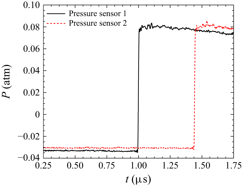

 X
 Ma
 R
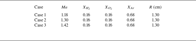
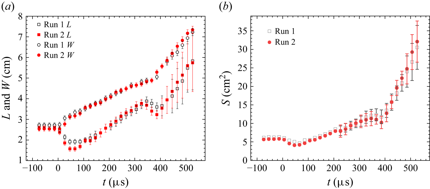
 L
 W
 S

 2

 L
 W
 S
 L/L0
 W/W0
 S/S0
 0
 τ=10tV0/(Lx−R0)
 V0=Ma⋅apre
 apre
 Lx=150mm
 R0
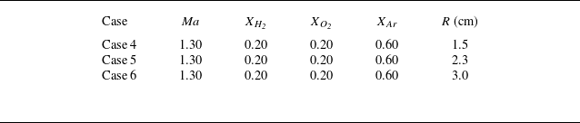


 L
 W
 S
 L/L0
 W/W0
 S/S0
 0


 Rmax
 Rmin
 R


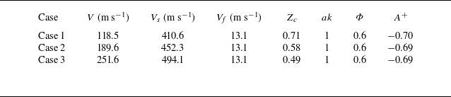
 V
 Vs
 Vf
 Zc=1−V/Vs
 ak
 Φ
 A+


 24.7%
 32.7%


 |uD|
 |uC|

 ρu
 Pu
 Tu
 σ
 σ=ρu/ρb
 SL
 lth
 δt
 (Tb−Tu)/|∂T/∂n|max
 δ
 δ=δt/lth
 Pr
 LeO
 LeF
 Le eff
 LeF
 LeO
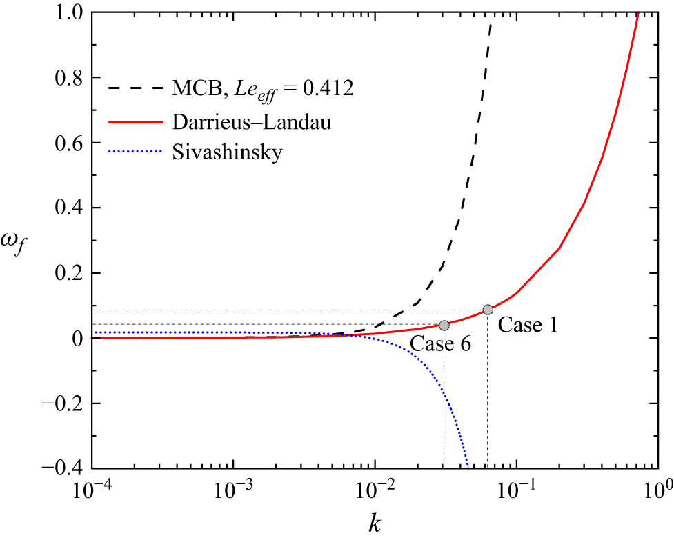
 k
 Le eff=0.412
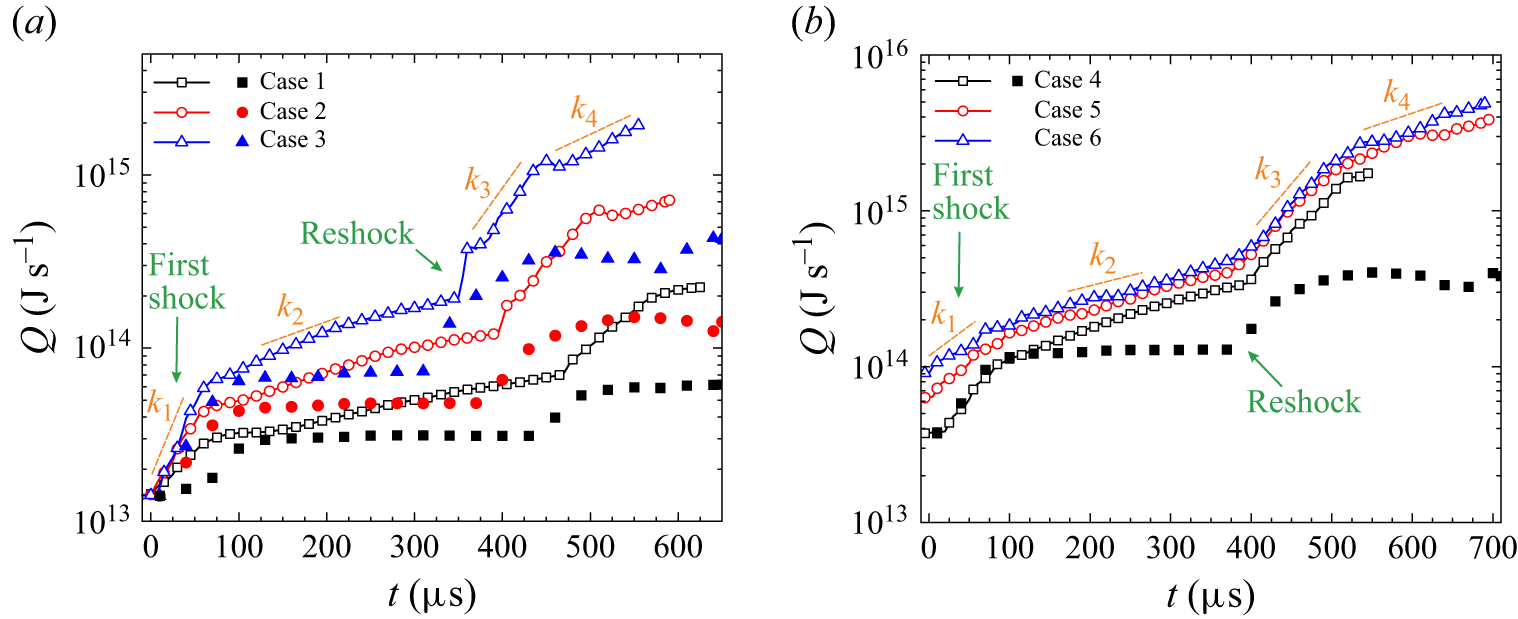
 k1
 k4
 lnQ∼kt

 X(H2)=0.159
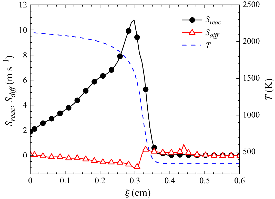
 t=145μs
 ξ
 S reac
 S diff
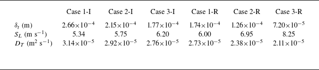
 δt
 SL
 DT
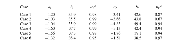
 i
 r
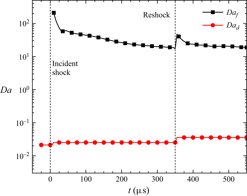
 Daf
 Dad
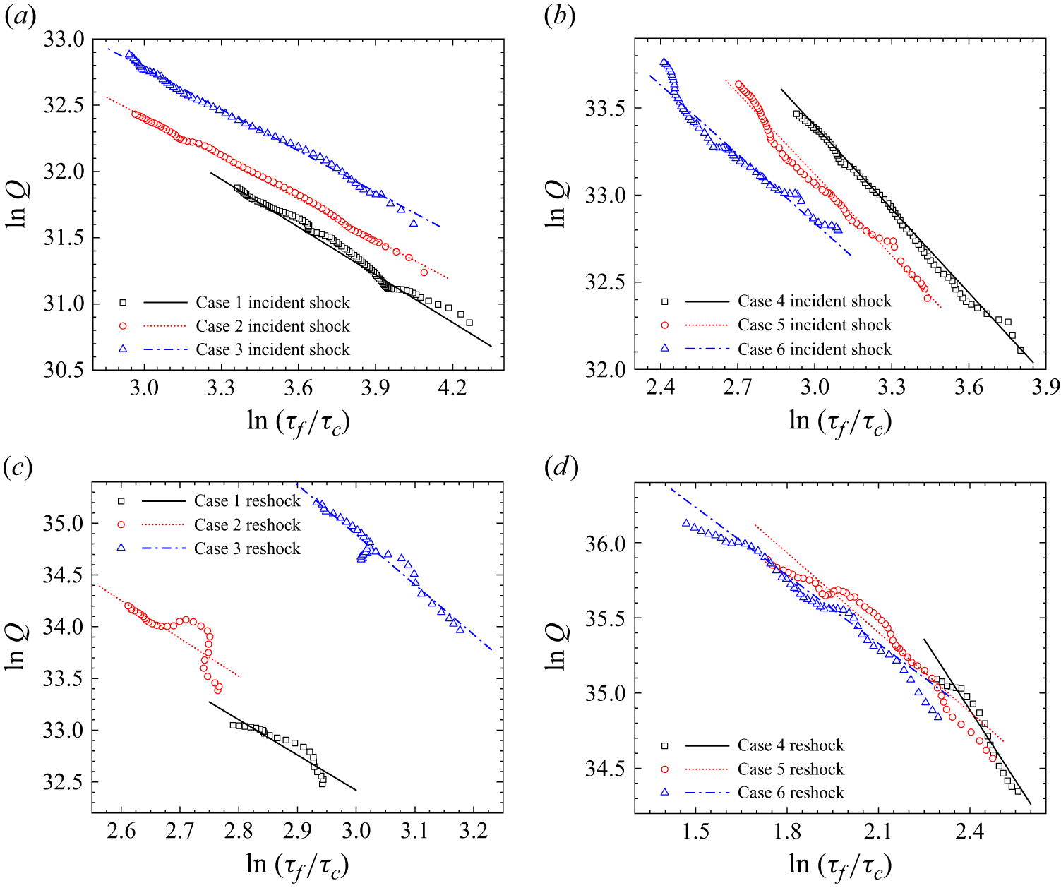
 τf/τc
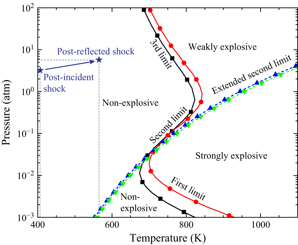
 2
 2
 2
 2
 X(H2:O2:Ar)=2:1:4
 X(H2:O2:Ar)=1:1:4.25
 X(H2:O2:Ar)=1:1:3