


“I am conscious that I have no equal in the art of swaying the masses.” —Adolf Hitler in a reported conversation (1932-34) with early copartisan Hermann Rauschning (Reference Rauschning1939). The authenticity of these records has been challenged; see Janssen (Reference Janssen1985).
PROLOGUE
On November 11, 1923, almost ten years before the Nazi seizure of power, Adolf Hitler was arrested and subsequently sentenced to five years in prison for his leading role in the Beer Hall Putsch, a failed coup d’état against the national government. While detained, Hitler ordered the banned and disintegrating National Socialist German Workers’ Party (Nationalsozialistische Deutsche Arbeiterpartei, NSDAP) to transform from a subversive battle group to a viable political party (Stachura Reference Stachura1980). As Hitler put it in a personal conversation with Nazi fundraiser Kurt Lüdecke (quoted in Pridham Reference Pridham1973, 27):
“Instead of working to achieve power by an armed coup, we shall have to hold our noses and enter the Reichstag [the national parliament] against the Catholic and Marxist deputies. If out-voting them takes longer than out-shooting them, at least the results will be guaranteed by their own constitution.”
Hitler was released on parole at the end of 1924 and caused the ban on the NSDAP to be lifted by affirming his party’s new loyalty to the constitution. His previous assertions notwithstanding, Hitler held a rabble-rousing public speech at the party’s relaunch on February 27, 1925 in Munich. The regional authorities’ reaction came swiftly: five forthcoming public appearances were cancelled immediately, and, on March 9, the Bavarian cabinet issued a two-year gag order against Hitler (Rösch Reference Rösch2002, 56–68). Many other regional governments, including those of Prussia, Saxony, Hesse, Oldenburg, Anhalt, Hamburg, and Lübeck, followed (Bruppacher Reference Bruppacher2012, 159–72). Although the NSDAP was not banned once again, party organs and meetings were subject to increased surveillance. According to police reports, turnout at NSDAP meetings and rallies declined markedly in the subsequent period (Rösch Reference Rösch2002, 208–10), and the NSDAP’s poor results at the state elections in Saxony, Mecklenburg-Schwerin, and Thuringia reinforced the view that “the NSDAP with a Hitler free to speak in public would cause no future concern to the authorities” (Pridham Reference Pridham1973, 77). On March 6, 1927, the Bavarian government revoked its gag order, and Adolf Hitler would take up his unprecedented campaign activities. In the period of time between the repeal of the speaking ban on March 6, 1927 and the eve of the Reichstag election of March 5, 1933, Hitler had 455 public appearances, with a gross estimated attendance of at least 4.5 million.Footnote 1 In only four years, the NSDAP evolved from a radical fringe group, garnering less than 3% of the vote at the 1928 Reichstag election, into the most popular German party, with more than 37% of the national vote in July 1932, effectively paving the way for the Nazi takeover in March 1933.
INTRODUCTION
After observing the influence Hitler seemed to wield through the use of propaganda, refugee-scholar Paul Lazarsfeld fielded a panel survey in Erie County, Ohio during the run-up to the 1940 U.S. presidential election. This marked the beginning of modern research into campaign effects (Hillygus Reference Hillygus, Leighly and Edwards III2010). The study’s findings were surprising—they did not substantiate Lazarsfeld’s motivating concern that campaigns could arbitrarily manipulate the public. Instead, the presidential campaign was found to merely activate the voters’ predispositions (Lazarsfeld, Berelson, and Gaudet Reference Lazarsfeld, Berelson and Gaudet1948). Subsequent studies came to similar conclusions (Berelson, Lazarsfeld, and McPhee Reference Berelson, Lazarsfeld and McPhee1954; Campbell, Converse, and Miller Reference Campbell, Converse and Miller1960) and entrenched the minimal effects paradigm that would dominate mass communication research for decades (Klapper Reference Klapper1960; Bennett and Iyengar Reference Bennett and Iyengar2008). In a way, however, the bulk of early empirical work focused on a least likely case. As Iyengar and Simon (Reference Iyengar and Simon2000, 151) note, identifiable net effects should be limited to highly unbalanced campaigns in which one candidate has a clear resource or skills advantage—a condition that is rarely met in U.S. presidential campaigns (also see Gelman and King Reference Gelman and King1993). Hitler’s campaign, by contrast, far exceeded any of his rivals’ efforts; the manipulative techniques employed were novel and sophisticated, and the use of modern technology, such as aircraft and loudspeakers, guaranteed Hitler an unparalleled geographic penetration and public attention (Paul Reference Paul1990). Tentative evidence for strong effects is indeed compelling: the numerous gag orders already speak volumes about the authorities’ beliefs in Hitler’s agitational potency, there were signs of electoral stagnation and organizational decay when the bans were in force, the unparalleled campaign activities that followed their repeal coincided with a steep electoral rise for the Nazi party, and plenty of reports from contemporary witnesses further corroborate the importance of Hitler’s campaign for the Nazis’ success (Abel Reference Abel1965).
Only a handful of studies have thus far attempted to systematically assess the effectiveness of early Nazi propaganda.Footnote 2 Most recently, Adena and her colleagues (Reference Adena, Enikolopov, Petrova, Santarosa and Zhuravskaya2015) measure local exposure to radio broadcasting using a method for predicting the spatial attenuation of radio signals. They find that exposure was negatively related to NSDAP support before the Nazi seizure of power and positively related soon afterward as the party assumed control over the mass media. In line with this finding, the authors also provide evidence that radio content before 1933 was largely pro-government and against the Nazis. These results corroborate the portrayal of early Nazi propaganda by later broadcasting director and Goebbels’ deputy Eugen Hadamovsky (Reference Hadamovsky1933, 44):
“All the means of public opinion were denied to Hitler. His newspapers were banned, he was denied use of the radio, his brochures and leaflets were confiscated. He had no choice but to reach the masses directly through constantly growing mass rallies.”
Ohr (Reference Ohr1997) collects data on local party events in Hessian communities and finds that in the period between the 1930 national and the 1931 regional parliamentary elections, there is a positive relationship in the changes of municipal Nazi vote shares. Wernette (Reference Wernette1974) also codes local Nazi election activities during the run-up to the 1930 Reichstag election from a national newspaper and finds a positive correlation with changes in municipal Nazi vote shares in the period 1928–1930. Ciolek-Kümper (Reference Ciolek-Kümper1976) focuses on Hitler appearances and—roughly—compares changes in ward-level Nazi vote shares at the regional election in Lippe on January 15, 1933 relative to the preceding Reichstag election in November 1932. She finds no evidence of the effectiveness of Hitler’s intense campaign efforts. Plöckinger (Reference Plöckinger1999) looks at differences between local- and regional-level Nazi vote shares at the July and November 1932 Reichstag elections in Bavaria but does not find any deviations between municipalities visited by Hitler and those that were not. Though inventive, the latter studies are limited in their geographic and temporal scope. They also potentially suffer from causality issues, which received much less attention at the time these studies were conducted than they do today.
In this study, we revisit the question of how effective early Nazi propaganda was in garnering electoral support in Weimar Germany. Our substantive focus is on Hitler’s public speeches as the Nazis’ chief campaign tool at that time. We rely on extensive original data that has superior geographic and temporal scope and resolution. We draw on the campaign resource allocation literature and use a semi-parametric difference-in-differences estimation strategy to account for often ignored endogeneity problems in the assessment of local campaign effects. In doing so, we also provide rare insight into the campaign strategy of the Nazi party. We discuss the limitations of our study and provide several robustness checks. Finally, we consider the implications of our findings for current research into campaign and leader effects.
ESTIMATING CAMPAIGN EFFECTS: PROBLEMS AND STRATEGIES
Campaign effects on voting behavior and election results are notoriously difficult to detect in a campaign realm characterized by the selective exposure of voters to a diffuse stream of countervailing campaign messages. Only since the late 1980s has the paradigmatic view of minimal campaign effects been challenged by scholars using novel data and sophisticated methodologies such as laboratory experiments (Iyengar and Kinder Reference Iyengar and Kinder1987), rolling surveys (Johnston et al. Reference Johnston, Blais, Brady and Crête1992), field experiments (Gerber and Green Reference Gerber and Green2000), and natural experiments (Huber and Arceneaux Reference Huber and Arceneaux2007).
While the historical perspective of our research precludes attractive design options that employ randomization or survey data,Footnote 3 a number of recent studies try to gauge the impact of campaign stops on voting behavior by using widely available information about the candidates’ campaign itineraries and local-level election results (Campbell Reference Campbell2008; Herr Reference Herr2002; Hill, Rodriquez, and Wooden Reference Hill, Rodriquez and Wooden2010; Holbrook Reference Holbrook2002; Jones Reference Jones1998; King and Morehouse Reference King, Morehouse and Schultz2004; Sellers and Denton Reference Sellers and Denton2006; Vavreck, Spiliotes, and Fowler Reference Vavreck, Spiliotes and Fowler2002). Such studies typically struggle with identification issues that challenge causal claims. Like any observational study, they are subject to potential confounding (see Goldstein and Holleque Reference Goldstein, Holleque and Leighley2010). Confounding would occur, for instance, if candidates and their staff deliberately selected locations for their appearances where they expected a large pool of easy-to-mobilize supporters or anticipated a close race. If a researcher failed to properly take into account such confounders (e.g., latent support, marginality), she would probably overestimate the effect of appearances on the candidate vote share and voter turnout.Footnote 4 We use a semi-parametric difference-in-differences estimation strategy to account for potential confounding due to observed and unobserved variables (see Abadie Reference Abadie2005; Heckman, Ichimura, and Todd Reference Heckman, Ichimura and Todd1997). In doing so, we specify a parametric model to predict the probability of Hitler appearances in a geographic unit and match visited units with control units that feature a similar predicted probability before the difference-in-differences analysis.
Beyond potential confounding, such studies of candidate appearances may be considered what epidemiologists call spatial ecological studies (Wakefield Reference Wakefield2004). Spatial ecological studies use geographic proximity to a presumed cause (in our case: campaign appearances) as a surrogate for individual exposure to the cause (attendance to the campaign event) and measure the response (voting behavior) at the level of geographic units (communities or counties).Footnote 5 A number of additional biases may arise in such a design. It is well known that group-level observations can be highly misleading when aggregate data are used to make inferences about individuals. Even under unconfoundedness (e.g., by random assignment of campaign appearances), we cannot unambiguously attribute higher turnout or voter support in visited localities to increased propensities among those who attended the campaign events to turn out and vote for the candidate. Such aggregate effects may also come about, for instance, in the fashion of an indirect two-step flow of communication (Katz and Lazarsfeld Reference Katz and Lazarsfeld1955), in which opinion leaders who would turn out and support their candidate anyway (i.e., for whom the individual effect of attendance is essentially zero) attend the event and are then motivated to mobilize and persuade others within their personal networks (Rosenstone and Hansen Reference Rosenstone and Hansen1993). In our particular case, positive effects of Hitler’s campaign visits on local Nazi vote shares might also have occurred indirectly through intimidation. As Childers and Weiss (Reference Childers and Weiss1990) document, violence was an integral part of Nazi mobilization strategy at the end of the Weimar Republic. If Hitler’s appearances were regularly accompanied by assaults on political opponents, increases in Nazi vote shares at the following election could have been the result of selective abstention by supporters of opponent parties. Either way, campaign effects on local-level election outcomes are, like other neighborhood effects, emergent properties of the social interaction of the residents (Oakes Reference Oakes2004). Therefore, one has to be cautious not to interpret even internally valid aggregate estimates of the effect of campaign appearances on election results in terms of the impact of individual attendance on voting behavior.
Finally, spatial ecological studies potentially suffer from ambiguities in separating exposure from nonexposure units. Effects of campaign events need not be restricted to the areal units for which we observe the outcomes of interest. For instance, voters and opinion leaders from neighboring units may also attend the events and thereby carry individual and network effects back home. Likewise, the geographic range of news media that cover the events may well exceed the borders of the units of analysis. Such spatial spillovers would violate the non-interference assumption underlying most methods for causal inference. Non-interference is an essential aspect of the stable unit-treatment value assumption (SUTVA), which implies that a treatment applied to one unit does not affect the outcome of other units. This allows researchers to employ multiple units for estimating causal effects (Rubin Reference Rubin1980). To illustrate the implications, imagine that Hitler’s appearances actually had their intended effect on Nazi support in the visited county, but that this effect carried over to neighboring counties through travel activity, personal networks, or media coverage. If these neighboring counties served as controls when assessing the effect of Hitler’s appearance on the NSDAP vote in the exposure county, the effect estimate would obviously be biased downward because the average overtime difference in outcomes among control units would not properly reflect the expected developments in the absence of the appearance. We, therefore, exclude neighboring areas from the pool of controls to account for possible spillovers.
THE TARGETING OF CANDIDATE APPEARANCES
In light of the potential confounding factors discussed above, the first step in assessing the impact of candidate appearances on election returns is to theorize how such visits are being targeted and in what way these factors relate to the outcome of interest (Althaus, Nardulli, and Shaw Reference Althaus, Nardulli and Shaw2002). In doing so, we adopt an instrumental view and assume that campaign activities serve to maximize votes while accounting for mobilization costs (Brams and Davis Reference Brams and Davis1974; Colantoni, Levesque, and Ordeshook Reference Colantoni, Levesque and Ordeshook1975; Cox Reference Cox1999). Candidates should focus their scarce resources accordingly—that is, on locations they expect personal appearances to favorably translate into additional votes, and specifically where additional votes would be decisive for winning mandates. The former suggests that rational campaigners primarily target locales with large numbers of eligibles and a high expected share of supportive voters. The latter expectation implies that candidates are more likely to visit competitive districts in which small vote shifts could change the allocation of mandates in their favor or to their detriment. All these factors—the number of eligibles, expected electoral support, and a party’s expected competitiveness—are potential confounders insomuch as they may also influence the outcome of interest. Applied to the present case, the size of the local electorate may be negatively linked to Nazi vote shares since rural areas were less populous and, at the same time, on average more supportive of the NSDAP than urban areas for programmatic reasons (Heberle Reference Heberle, Büsch, Wölk and Wölk1978; Thurner, Klima, and Küchenhoff Reference Thurner, Klima and Küchenhoff2015). Likewise, the classical decision-theoretic model of voting suggests that a party’s expected competitiveness may directly affect the relative strength of parties through selective participation and strategic voting (Cox Reference Cox1999).
Local infrastructure is also relevant to mobilization costs. In the context of U.S. presidential campaigns, Holbrook’s (Reference Holbrook2002) study of Truman’s 1948 whistle-stop campaign and Althaus, Nardulli, and Shaw’s (Reference Althaus, Nardulli and Shaw2002) narratives of the boat trips down the Mississippi river by Al Gore in 2000 and by George H.W. Bush in 1988 provide good examples of campaigns in which ground transportation connectivity mattered. A remarkable feature of Hitler’s 1932 campaign was that, for the first time in history, he chartered a plane to transport him to certain campaign events. Under the ambiguous label “Hitler over Germany,” he made nearly 150 appearances from April until November 1932. Therefore, distance to the nearest airfield should have mattered for targeting event locations starting with the 1932 elections. The strength of local party organizations is often quoted as an important source of logistic support and secondary mobilization (Cox Reference Cox1999; Rosenstone and Hansen Reference Rosenstone and Hansen1993). Some authors even consider local organizational strength as another campaign tool subject to strategic allocation (Bartels Reference Bartels1985), which reminds us that a leading candidate’s campaign is not a unitary entity but rather a set of efforts undertaken by various agents. For instance, Kelley (Reference Kelley and David1961) found in his study of U.S. presidential campaigns that contenders used their running mates’ schedules in either complementary or duplicative ways. Geographically or temporally complementary campaign schedules carry the risk of offsetting campaign effects (Finkel Reference Finkel1993), while duplicative itineraries bring about potential misattribution of campaign effects. One way or the other, we need to account for the activities of other Nazi speakers when assessing the effects of Hitler’s public appearances. The following section introduces measurements for all relevant confounders.
DATA COLLECTION AND MEASUREMENT
Period of observation. Our empirical analysis covers the period between the repeal of the speaking ban on Hitler in Bavaria on March 6, 1927 and the last (halfway) competitive Reichstag election on March 5, 1933.Footnote 6 Five national parliamentary elections (on May 20, 1928; September 14, 1930; July 31, 1932; November 6, 1932; and March 5, 1933) and a two-round presidential election (on March 13, 1932 and April 10, 1932) were held within this period. Our difference-in-differences approach focuses on changes between the four consecutive parliamentary elections and both rounds of the presidential election, respectively.
Areal units. The availability of election statistics dictates our choice of areal units. Thanks to a data collection effort of epic proportions by Jürgen Falter and collaborators (Falter and Hänisch Reference Falter and Hänisch1990), digitalized community-level election statistics are available for the 1928, 1930, and 1933 elections; however, they are not available for the elections in 1932, whose results the Reich Statistical Office (Statistisches Reichsamt) reported only for the higher administrative levels of counties (Kreise) and county boroughs (kreisfreie Städte) (see Hänisch Reference Hänisch1989, 45). This leaves us with a single election pair (1928–1930) for a community-level difference-in-differences analysis. We will use the community-level data (N = 3, 864), among other things, to check the sensitivity of our empirical results for potential violations of the non-interference assumption discussed above. Other than this, our analytical focus will be on the counties and county boroughs (N = 1,000). While election statistics are available at the county and, partly, the municipal level, neither level was relevant for the apportionment of parliamentary seats. Mandates were allocated at the level of the 35 primary districts (Wahlkreise) and 16 secondary districts (Wahlkreisverbände), which will serve as additional geographical layers to compute measures of the NSDAP’s competitiveness.
Areal units are key in generating and combining substantive variables. Unfortunately, the Falter data do not readily contain the geographic information necessary to do so.Footnote 7 In an independent data collection effort, we retrieve the center coordinates of the municipalities and county boroughs included in Falter and Hänisch (Reference Falter and Hänisch1990) from the Google Maps API service (Google Inc. 2015). Whole counties are georeferenced in terms of the center coordinates of their main towns or cities to account for the uneven population distribution within counties. Details and links to computer code can be found in Appendix A.
Outcome variables. The primary outcome of interest is the number of NSDAP votes in a Reichstag election in an areal unit relative to the voting-eligible electorate. The reason for standardizing against the number of eligible—not actual—voters is that the specific apportionment method used in Reichstag elections guaranteed each party one seat per 60,000 votes (see Appendix E). Therefore, an increase in the number of votes from one election to the next would increase a party’s chances of winning additional seats irrespective of the vote gains and losses for other parties. We also use the vote share of the communist party (Kommunistische Partei Deutschlands, KPD) as the Nazi’s major adversary and the turnout rate as alternative outcomes. For the 1932 presidential elections, we use vote shares for Adolf Hitler and Ernst Thälmann, the KPD’s candidate, as outcomes of interest. The relative size of the areal units’ voting-eligible population serves as a weighting variable in the difference-in-differences analysis. Given its vast variability across units—county-level electoral populations range between 184 and 871,764, with a mean of 41,358 eligibles—appropriate weights are imperative for our analysis (Ridgeway et al. Reference Ridgeway, Kovalchik, Griffin and Kabeto2015). All election data are taken from Falter and Hänisch (Reference Falter and Hänisch1990).
Exposure. Our main source of information about Hitler’s public appearances is the multivolume edition “Hitler. Reden, Schriften, Anordnungen” (Hitler. Speeches, Writings, Directives) by the Institute for Contemporary History Munich (Hitler Reference Hitler1992, Reference Hitler1994a, Reference Hitler1994b, Reference Hitler1994c, Reference Hitler1995, Reference Hitler1996, Reference Hitler1997, Reference Hitler1998). For each appearance within the specified period, we hand code its date, location, type of event (public or private) and, if available, attendance figures by source (police reports, press coverage, Nazi press coverage). As the edition only covers the period until Hitler’s appointment as head of the national government on January 30, 1933, we consult Bruppacher (Reference Bruppacher2012) to fill the gap until the Reichstag election on March 5, 1933. For validation we use Bruppacher (Reference Bruppacher2012) and Domarus (Reference Domarus1973) and retrieve information from hitlerpages.com, a website maintained by a Dutch amateur historian that provides a daily account of Adolf Hitler’s life compiled from various sources. In sum, we are able to identify 566 Hitler appearances in the specified period, 455 of which were public.Footnote 8 Figure 1 provides a timeline of events for the entire observation period.Footnote 9 Apparently, Hitler’s campaign activities had already been intense in the period between the 1928 and 1930 elections (84 appearances) and culminated in the run-up to the 1932 presidential and Reichstag elections (243 appearances). In early 1933, as Hitler had already been appointed head of government, the NSDAP’s strategy quickly switched from winning votes to repression (Evans Reference Evans2005). Of the meager 36 events recorded between November 7, 1932 and March 5, 1933, as many as 16 related to the January 15, 1933 regional elections in Lippe.Footnote 10
Timeline of Hitler’s public appearances, March 1927 to March 1933.

To assess the effect of Hitler’s appearances on local election returns, we would ideally know whether or not (or rather: to what extent) the local population for which we observe the outcome had been exposed to the event. This information is simply not available. Like other spatial ecological studies, we use spatial proximity to the events as a surrogate for exposure. First, Hitler appearances are point-referenced according to their location (municipality or borough center, possibly even the specific venue) using the Google Maps API service. We then classify those counties and county boroughs (municipalities in the municipal-level analysis) whose center coordinates were situated within a radius of ten kilometers from an event location at any time during an interelection period as exposure units. Alternative specifications of the exposure variable with varying geographical and temporal scope will be considered in the section on robustness.
Competitiveness. The rational-actor perspective suggests that Hitler and the NSDAP focused their scarce campaign resources on close races—that is, on electoral districts where the stakes of winning additional seats and of losing seats won in previous elections were high. To measure the NSDAP’s local electoral stakes, we follow lines similar to Grofman and Selb (Reference Grofman and Selb2009) and develop party-specific competition indices that are sensitive to the nature of the automatic apportionment method used at that time (Schanbacher Reference Schanbacher1982). The indices are specified at the level of the primary and secondary electoral districts (Competitiveness 1 and 2, respectively). They reflect the minimum vote distance of the NSDAP to winning an additional seat or to losing their final seat at the respective level at the previous election relative to the highest possible vote distance to a seat gain or loss. An index value of one indicates maximum competitiveness, a value of zero indicates the theoretical minimum. Details of the calculations and descriptive statistics are given in Appendix E.
Organizational strength. It has been argued that local infrastructure is relevant to mobilization costs and that the strength of local party organization is one important infrastructural factor. Apart from some regional studies (Anheier Reference Anheier, Diani and McAdam2003; Anheier, Neidhardt, and Vortkamp Reference Anheier, Neidhardt and Vortkamp1998), there is no systematic nationwide information about the local organizational strength of the NSDAP and its development over time. As a proxy for organizational strength, we estimate county-level party membership totals (in 1,000) based on samples drawn from the two original NSDAP member files archived at the Berlin Document Center by teams of researchers in Berlin (Falter and Kater Reference Falter and Kater1993) and Minneapolis (Brustein Reference Brustein1998). The sample data include, inter alia, information about the place and date that the members joined. The thorough description of the sampling procedures in Schneider-Haase (Reference Schneider-Haase1991) allow us to calculate appropriate design weights. Unfortunately, the researchers used fixed yearly quotas for entries in the period 1930–1933 so that it is impossible to calculate time-varying weights. Auxiliary information about the annual development of national membership figures from Kater (Reference Kater and Mann1980) is used to generate election-specific estimates. Details of the estimation procedure and descriptive statistics are given in Appendix F.
Distance to nearest airfield. Of particular importance for mobilization costs as of 1932 is the distance to the nearest airfield. We consult several Wikipedia entries and a privately run websiteFootnote 11 to identify a total of 70 civilian airfields in operation at that time. We use the Google Maps API service to geocode the airfields, which provides the basis for calculating minimum distances to an airfield (in 100 km) for each municipality, county borough, and county. Figure G1 in the Appendix maps the location of the airfields as well as the minimum distances.
Number of eligibles and previous vote share. Our theoretical considerations suggest that rational campaigners primarily target locales with large numbers of eligibles and a high expected share of supportive voters. Therefore, we include the number of eligibles (in 100,000) and the vote share of the NSDAP (for the 1932 presidential election: Hitler) at the previous election (i.e., the first election in each election pair considered). Information on both variables is taken from Falter and Hänisch (Reference Falter and Hänisch1990).
Goebbels’ appearances. To account for the eventuality that Hitler’s campaign schedule was complemented or duplicated by those of other high-profile Nazi speakers, we collect information about the public appearances of Joseph Goebbels, the second most important Nazi speaker after Hitler. We first conduct an automatic search of keywordsFootnote 12 using a digital version of his diaries (Goebbels Reference Goebbels1992) and then manually code information on places, dates, and types of speeches (public or private). Finally, we geocode the appearances using the Google Maps API service. In total, we are able to collect data on 200 public speeches, an overwhelming majority of which (110) were held in Berlin. Figure B2 in the Appendix maps the locations of Goebbels’ appearances.
Previous appearances. In addition to the matching variables listed, we include a binary variable that indicates whether Hitler previously (i.e., before the last election) visited a county to help control for unobserved confounders, assuming that those factors had already affected past targeting decisions. Election-specific summary statistics of all the variables and supplementary maps are given in Appendix H.
PREDICTING HITLER’S APPEARANCES
In the first stage of our empirical analysis, we model the election-specific probability of a Hitler visit to a community or county as a function of the above covariates. Predictions from these models will then be used in the causal inference step to trim the sample to include as controls only those counties and communities that are similar to exposure units in terms of their estimated propensity score (while also being geographically distant enough from exposure units). The results from the propensity score estimation are interesting in their own right, too, since they provide rare systematic insight into early Nazi campaign strategy. While there are numerous studies on the organization of Nazi propaganda (e.g. Anheier Reference Anheier, Diani and McAdam2003; Rösch Reference Rösch2002) and the manipulative techniques employed (e.g. Anheier, Neidhardt, and Vortkamp Reference Anheier, Neidhardt and Vortkamp1998; Paul Reference Paul1990), little is known about the targeting of candidate appearances.
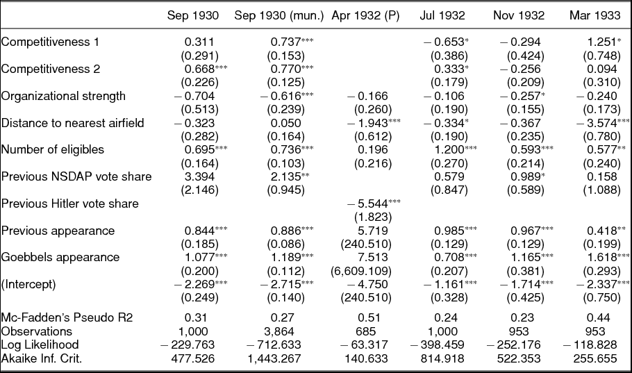
Table 1 reports probit estimates and their standard errors (clustered by primary electoral district) for each election separately. As one would expect, the size of the eligible voting population in a county turns out to be a consistent predictor of Hitler’s campaign appearances across elections. Also in line with our expectations, the distance to the nearest airfield is a significant predictor of Hitler visits as of the 1932 elections—Hitler’s first campaign trip by plane did not occur before April 3, 1932 (Bruppacher Reference Bruppacher2012, 265). The exceptionally large coefficient on airfield distance referring to the 1933 election is due to the extraordinarily intense regional election in Lippe in January 1933 and its proximity to the airports of Bielefeld and Hannover-Vahrenwald (see Figure H2 in the Appendix). The campaign trail also tended to stop where the NSDAP did well in the previous election—although the coefficients are, at most, weakly significant—and where the last election was close from the party’s viewpoint. The parameter estimates indicate a negative relationship between the strength of local party organizations and the probability of a visit. An ad hoc interpretation of this finding would be that Hitler appearances were targeted at areas lagging behind in terms of organizational development to increase party membership (see Bytwerk Reference Bytwerk1981, 16). Unfortunately, the available samples from the NSDAP member files are too small to detect local changes in membership in the immediate aftermath of Hitler appearances. What additional analyses show, however, is that local organizational development in the whole legislative period following an election did not systematically differ between exposure and nonexposure units.Footnote 13. The significantly positive coefficient associated with Goebbels’ appearances suggests that Goebbels’ campaign schedule tended to duplicate Hitler’s. Thus, if we ignored Goebbels’ activities, there would be a risk in the subsequent analyses of erroneously ascribing campaign effects to Hitler, whereas they actually trace back to Goebbels. Finally, previous campaign appearances prove to be useful predictors of current events, indicating that there are factors relevant to (past and current) targeting choices that are not appropriately taken into account in our model specification.Footnote 14 Nevertheless, the models fit the data remarkably well. Pseudo R2 values range between 0.23 in November 1932 and 0.51 in April 1932. That is, Hitler’s campaign schedule appears to be pretty much in accord with an instrumental account of campaign resource allocation. Further, there does not seem to be much variation in campaign strategy over time.
Probit estimates of Hitler appearances by election. Standard errors in parentheses.

Note: *p<0.1; **p<0.05; ***p<0.01
MATCHING AND COVARIATE BALANCE
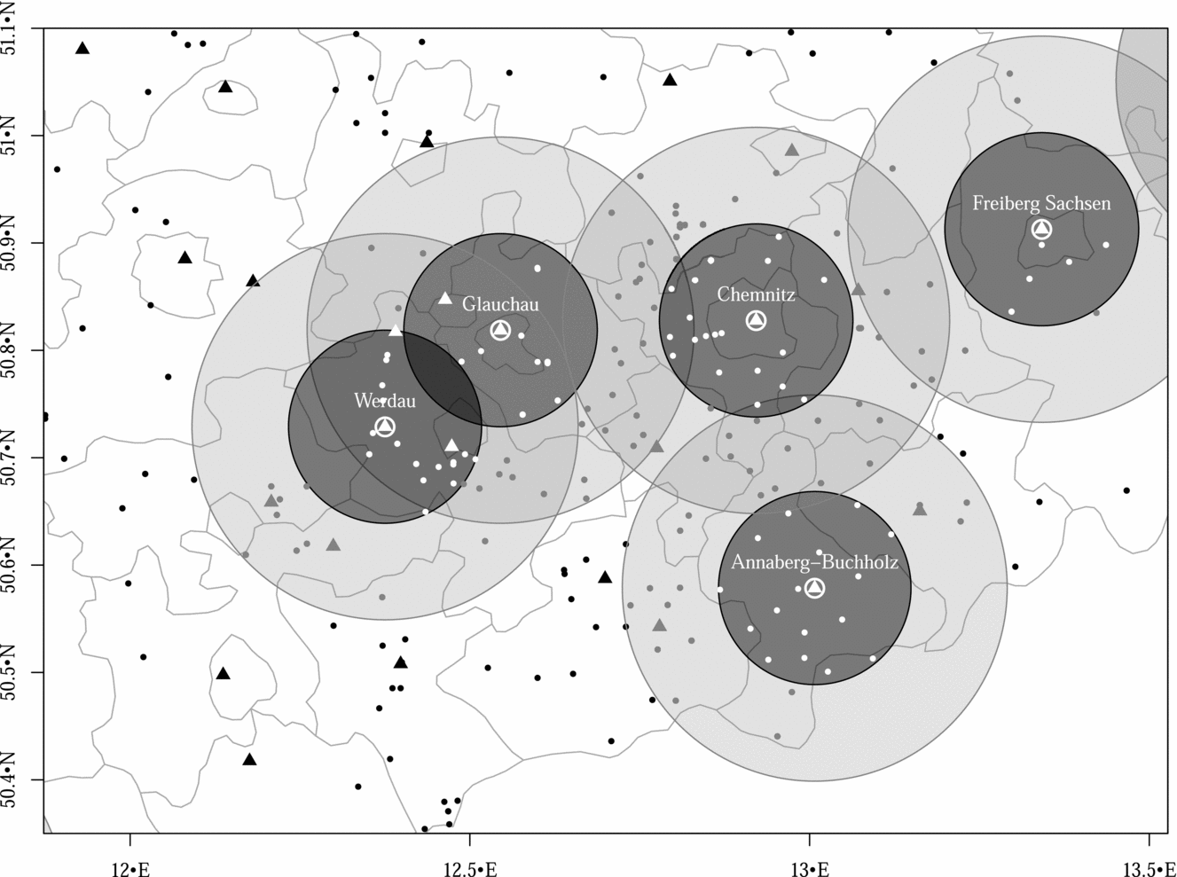
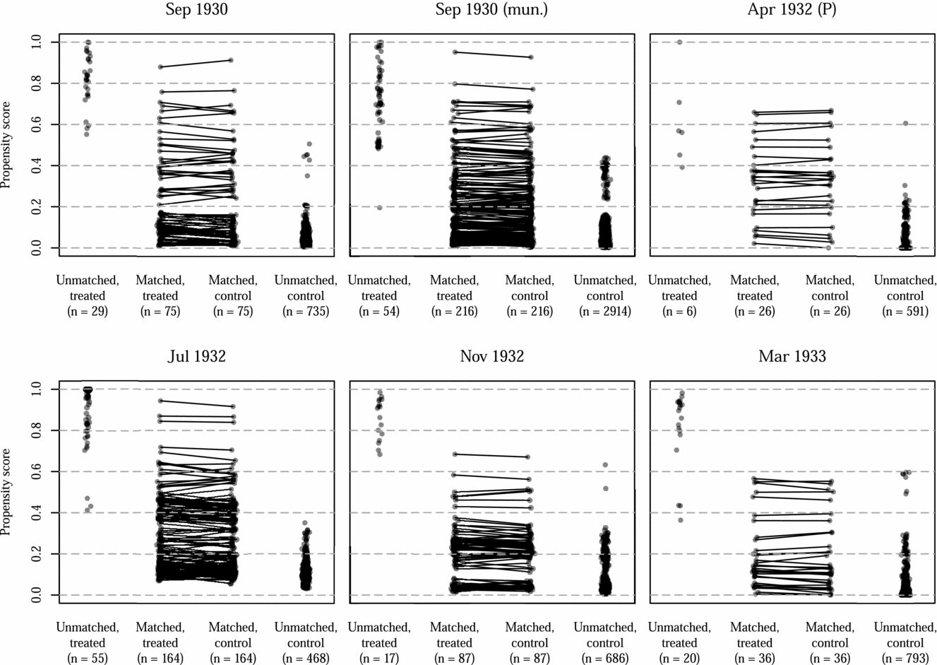
There are a variety of matching methods available. The decision of which to choose from among them involves balancing the tradeoffs inherent in each between variance and bias (Caliendo and Kopeinig Reference Caliendo and Kopeinig2008). Our preferred method is 1:1 nearest-neighbor matching without replacement subject to a caliper constraint of 0.25 standard deviations on the estimated propensity score. As an additional restriction, we draw no-matching areas of ten kilometers around the exposure units and only match control units outside these areas to safeguard our analysis against potential spillover effects. The definitions of exposure, no-matching, and potential control areas are illustrated in Figure 2. The matching results are illustrated in Figure 3. On one hand, the method throws away a nontrivial amount of information from both the pool of potential controls and the exposure group, which may result in loss of statistical efficiency. On the other hand, expanding the caliper and/or oversampling controls for efficiency gains may increase bias in matching estimators due to the inclusion of poorer matches.Footnote 15
Illustration of radius definitions of exposure areas (dark grey; event locations in white), no-matching areas (light grey), and potential control areas (white; potential control units in black). Triangles represent centers of county boroughs. Dots represent municipal centers.

Predicted propensity scores by exposure and matching status. Lines indicate matched pairs.

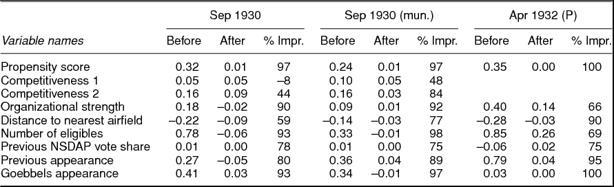
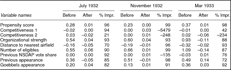
Tables 2 and 3 report mean differences in variables between exposure and control units before and after matching plus a statistic that indicates the relative improvement of covariate balance through matching. Matching markedly improved covariate balance to the extent that there are barely any mean differences left. The seemingly curious instances of covariate balance deteriorating after matching occur in situations in which the distribution of variables was well balanced before matching. In these cases, slight distributional changes had massive consequences for the—relative—improvement statistic. Overall, the balancing statistics suggest that we can approach the causal analysis step with a certain measure of confidence, at least with regards to the observed potential confounders.
Propensity score and covariate balance before and after matching. Mean differences on variables reported.

Propensity score and covariate balance before and after matching, continued. Mean differences on variables reported.

ESTIMATING CAMPAIGN EFFECTS: EMPIRICAL RESULTS
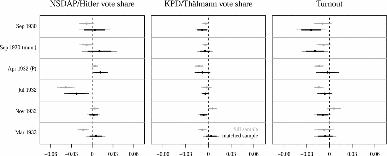
The semi-parametric difference-in-differences estimate of the effect of Hitler appearances is the mean difference in the overtime changes of outcomes between the matched exposure and control units, with each unit weighted according to the size of its electoral population. Difference-in-differences estimation critically rests on the assumption that observed overtime changes in the control group reflect, on average, unobserved changes in the exposure group in the absence of treatment. A common plausibility check of such parallel trends is to compare pretreatment changes over time between exposure and control units. Figure I1 in the Appendix does not indicate any differences in pre-treatment developments for the 1932 and 1933 Reichstag elections.Footnote 16 Figure 4 reports difference-in-differences estimates for the five election pairs and their 80% and 95% confidence intervals, both for the matched and unmatched samples. The calculation of confidence intervals is based on robust standard errors to account for the clustering of temporal observations (pre- and post-exposure) within areal units. Results for three outcomes are reported: NSDAP (Hitler) vote shares, KPD (Thälmann) vote shares, and turnout. Most point estimates are in the range of ±1% of the voting-eligible population, and hardly any coefficient is significantly different from zero at conventional probability levels. The strongest effect of −2.4% pertains to electoral turnout in the 1928–1930 election pair, indicating that Hitler’s early appearances had, on average, a demobilizing effect in exposure areas. A look at the other outcomes suggests that this demobilizing effect tended to harm the KPD but left the Nazi (population) vote share unaffected. This result supports Childers and Weiss’s (Reference Childers and Weiss1990) observation that a concomitant feature of Nazi campaign events was concerted violence to intimidate political opponents and their supporters. This specific empirical pattern disappears in later elections, perhaps indicating that Goebbels’ attempt to align the paramilitary branch of the NSDAP (Sturmabteilung, SA) to the quasilegal course adopted earlier was, at least in part, successful. Although estimated exposure effects on NSDAP vote shares are mostly zero, a negative effect occurs with the 1930–32 election pair—just when the Nazis took their greatest leap forward electorally!
Difference-in-differences estimates of exposure effects on NSDAP (Hitler) vote shares, KPD (Thälmann) vote shares, and turnout in national parliamentary and presidential elections 1930–33. Lines represent 80% and 95% confidence bands. Estimates are reported for unmatched and matched samples. For full model statistics, see Tables I1 to I3 in the Appendix.

The 1932 presidential runoff election deserves special mention. Incumbent president Hindenburg had emerged as the clear front-runner from the first election round on March 13, 1932, garnering 49.5% of the vote. By comparison, Hitler won 30.1% of the vote, and communist leader Ernst Thälmann secured 13.5%. All other candidates combined received less than 7%Footnote 17 and did not stand again in the decisive second round. Hindenburg, who did not bother to enter the electoral fray himself (Pyta Reference Pyta2007, 475), issued an emergency decree that limited the campaign period preceding the runoff on April 10 to just the six days prior to the election—a decision that prompted Hitler to utilize the airplane for the first time as a means of transportation for campaigning. The novel mode of transportation afforded him 21 campaign appearances spread over the whole country during this short period, with a maximum of five appearances per day. Even though Hitler eventually lost the election to Hindenburg, he still gained more than two million additional votes from the first to the second round. Our analysis suggests that some of the vote gains actually came from his campaign appearances. The finding that an unusually short and intense campaign had significant effects is in line with results from previous research, which indicates that campaign effects run out quickly over time (e.g., Watt, Mazza, and Snyder Reference Watt, Mazza and Snyder1993)—for example, due to the interference of offsetting campaign messages. To more systematically account for potential effect decay, we replicated our analysis, but this time only considering campaign appearances that took place within two, four, eight, and twelve weeks before an election. The results are, however, inconclusive. The details are reported in Tables I7 to I21 in the Appendix.
A final methodological remark, the matching approach obviously makes a difference. Difference-in-differences estimates of exposure effects on Nazi vote shares are consistently more negative when applied to the unmatched samples. This indicates that Hitler’s campaign trail usually stopped where smaller increases (or larger decreases) in NSDAP vote shares were to be expected. One interpretation of this result would be that, for infrastructural reasons, Hitler’s appearances were scheduled in more populous urban areas where the NSDAP tended to fare worse electorally for social structural and programmatic reasons (Heberle Reference Heberle, Büsch, Wölk and Wölk1978; Thurner, Klima, and Küchenhoff Reference Thurner, Klima and Küchenhoff2015).
ROBUSTNESS
Absence of evidence is no evidence of absence. In this section, we will play devil’s advocate and ask if there are reasons to suspect that actual campaign effects went undetected with our data and research design. The discussion is organized around three potential problems: SUTVA violations due to spatial spillovers and multiple versions of exposure, violation of the causal transience assumption with respect to previous Hitler appearances, and the limitations of our data and inferential approach to identify the effects of dynamic campaign strategies.
Spatial Spillovers and Multiple Versions of Exposure
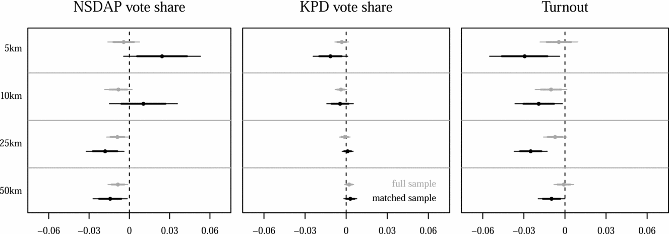
One serious drawback of our study is the nonavailability of exposure data. Like other spatial ecological studies, we have to make do with spatial proximity to events as a surrogate for exposure. Thus far, the specification of the exposure variable has arbitrarily fixed the geographic reach of Hitler appearances to a radius of ten kilometers around venues. If the actual reach of events was wider than that, campaign effects might have spilled over to neighboring areas that served as potential comparison units in estimating (in this case, underestimating) effects (see Rubin Reference Rubin1980). In the previous analysis, we drew no-matching zones around exposure areas to avoid this problem. As an alternative, we now vary the specifications of exposure areas from five to 50 kilometers around event locations for the 1928–1930 municipal-level data, which provide the highest spatial resolution. We likewise vary the range of the no-matching zones from five to 50 kilometers. The results plotted in Figure 5 indicate that initially positive effects of visits on NSDAP vote shares as well as initially negative effects on communist vote shares and turnout tend to fade out with increasing spatial distance. While these findings do not immediately suggest an optimal cutoff value for specifying exposure areas, our hunch is that a radius of 10 km plus an additional 10 km no-matching zone is a safe choice. The potential for even broader diffusion effects (e.g., through national media) seems limited given the Nazis' limited access to public media; its mostly negative stance toward Hitler before 1933 (Adena et al. Reference Adena, Enikolopov, Petrova, Santarosa and Zhuravskaya2015); the low circulation figures of the Nazis’ own national paper, Völkischer Beobachter (Layton Reference Layton1970); and the geographically fragmented press landscape at that time (Führer Reference Führer2008).
Difference-in-differences estimates of exposure effects on alternative outcomes at the 1930 national parliamentary election (municipality-level data). Specifications of exposure areas vary from five to 50 km around venues. Lines represent 80% and 95% confidence bands. Estimates are reported for unmatched and matched samples. For full model statistics, see Tables I4 to I6 in the Appendix.

Apart from non-interference between units, SUTVA also requires that there be only a single version of treatment (Rubin Reference Rubin1980). This assumption is unlikely to hold in the present case for at least two reasons. First, the number of Hitler appearances between elections differed between exposure counties and elections. While most of the exposure cases (66%) actually reflect single campaign visits, there are other instances in which Hitler made multiple appearances in the run-up to an election. To name just the most extreme cases, Hitler held 17 public speeches between the July and November Reichstag elections of 1932 in Berlin-Mitte; for Munich, the hometown of the Nazi movement, this figure was 37! To account for varying numbers of campaign events, we have replicated our matched difference-in-differences analysis for each of three exposure levels (see Imbens Reference Imbens2000): one, two, and three or more campaign appearances.Footnote 18 The results, which are detailed in Table I22 in the Appendix, do not point to any systematic differences between exposure levels. Second, the size of events also varied widely. The figures range from 400 on November 30, 1928 in a gym in Hersbruck to an estimated 100,000 on July 20, 1932 at the Victoria sports field in Hamburg, with an average of about 15,000 attendees. The problem of ignoring varying event size is, again, one of hidden variation of treatments. Larger events may have had stronger effects because they had reached a wider audience of voters and opinion leaders or because they had attracted more media attention, through which the campaign messages were promulgated to the wider public. Larger events could have also increased the intensity of spatial spillovers through both travel activities and local press coverage. Once again, additional analyses do not indicate any systematic differences among events with less than 5,000; 5,000–20,000: more than 20,000 attendees; and of unknown event size, respectively. In a related manner, we also looked for differences across counties with eligible voting populations of less than 20,000; 20,000–50,000; 50,000–80,000; and more than 80,000—again without any notable differences. The detailed results are reported in Tables I23 to I35 in the Appendix.
Causal Transience
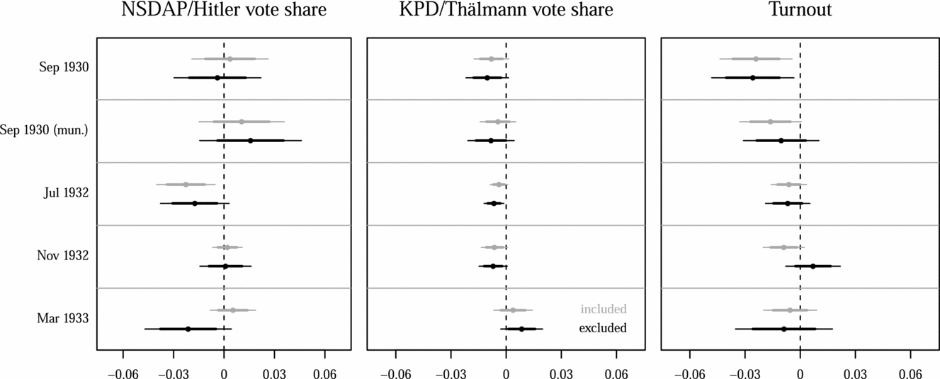
Our difference-in-differences estimation hinges on the causal transience assumption, namely that the electoral response to a Hitler visit in a given period is not affected by prior visits in that area (see Holland Reference Holland1986). This assumption is particularly critical since our propensity score model includes previous Hitler appearances among the predictors to account for unobserved factors that guided targeting decisions. Therefore, chances are that we end up matching previously visited exposure areas with previously visited controls. If visits had their intended electoral effect, but this effect was nontransient in time and noncumulative over repeated events (see the preceding section), then we would underestimate the effect of current events. While our earlier findings in connection with the 1932 presidential election do not point toward persistent effects, an additional matching analysis in which we exclude areal units that had already been exposed to Hitler appearances in the preceding election period provides a more direct check for the credibility of causal transience. As previous appearance is a powerful predictor of current appearance, most of the excluded matches come from the high- and intermediate-propensity domain (see Figure I5 in the Appendix). Figure 6 contrasts effect estimates from this analysis (in black) with our main results (in grey) from Figure 4. The 1932 presidential runoff had to be altogether excluded from the comparison since Hitler had already visited all but one of the 21 venues previously. Naturally, the elimination of matched pairs involving previously visited areas leads to wider confidence bands, but there are no notable differences to our main findings beyond this. This result lends some tentative support for causal transience to hold.
Difference-in-differences estimates of exposure effects on NSDAP vote shares, KPD vote shares, and turnout in national parliamentary elections 1930–33. Lines represent 80% and 95% confidence bands. Estimates are reported with previously visited areas included and excluded. For full model statistics, see Tables I36 to I38 in the Appendix.

Dynamic Campaign Strategies
It is a small step from the instrumental actor’s perspective, which guides the selection of covariates for the propensity score model, to the notion of dynamic strategies, according to which candidates continuously adapt their actions in response to campaign events and opponents’ actions. To take an example, Plöckinger (Reference Plöckinger1999, 73–7) reports increased activity of local NSDAP organizations and their foes ahead of Hitler’s visits—leafleting on both sides, bill-posting and over-painting, and sabotage—which may have all affected the vote in different ways. Blackwell (Reference Blackwell2013) exposes the problem of one-shot methods for causal inference to separate actions from reactions. This distinction is important since causes of the actions of interest (i.e., Hitler speeches) are relevant confounders to be taken care of when assessing their causal effect, while conditioning on the consequences of these actions “controls away” relevant indirect parts of their effect. A solution to this problem is to investigate the effect of an action sequence on an outcome using methods for dynamic causal inference (Robins, Hernán, and Brumback Reference Robins, Hernán and Brumback2000). Unfortunately, we do not have any nationwide information about the campaign activities of other parties and candidates, much less about seemingly spontaneous actions as those reported above.Footnote 19 Therefore, our analysis—thus far tacitly—proceeded on the assumption that while Hitler might have recalibrated the content of his speeches in response to campaign events and opponent actions, his itinerary had been fixed at the beginning of a campaign. Several entries in chief strategist Goebbels’ (Reference Goebbels1992) diaries suggest this was actually the case. If, on the other hand, Hitler’s speeches provoked counteractions by opposing parties or back-up measures by supporters in the manner reported by Plöckinger (Reference Plöckinger1999), we would still be able to conclude that the overall effects of Hitler’s appearances were essentially zero. Yet another threat to valid inference would arise if “regular” campaign events organized by local branches of the Nazi party and Hitler visits were planned in a complementary fashion, which would have led to their purportedly positive effects cancelling each other out in the analysis. However, the event calendars of the Lippe campaign in December 1932 and January 1933 published in Ciolek-Kümper (Reference Ciolek-Kümper1976, 313–7) suggest that Hitler’s appearances were normally scheduled in addition to the list of district or regional speakers.
In any case, it is important to keep in mind that we are examining the effect of Hitler’s appearances on top of other campaign activities by the Nazis and their competitors. The lack of data on these activities inevitably needs to be compensated with—hopefully plausible, but at the very least explicit—assumptions about their targeting.
CONCLUSION
Our empirical analysis suggests that Hitler’s speeches as the Nazis’ chief campaign tool at the end of the Weimar Republic were rationally targeted toward populous, competitive, and accessible areas, yet their electoral effects were modest at best and of limited geographical and temporal scope. The only significantly positive effect occurred with the 1932 presidential runoff—an election preceded by an extraordinarily short, intense, and one-sided campaign. The effect was far too feeble, however, to swing the election in Hitler’s favor.
This result is particularly remarkable evidence for a qualified view of the effectiveness of election campaigns to manipulate the public (e.g., Campbell Reference Campbell2008; Gelman and King Reference Gelman and King1993; Popkin Reference Popkin1991) since several important ingredients that are commonly claimed to create communication environments conducive to substantive campaign effects were present at the time: Hitler relied heavily on personal appearances, even today considered by campaign practitioners as one of the most potent ways for candidates to directly shape public opinion while avoiding the often negative tone of the media (Althaus, Nardulli, and Shaw Reference Althaus, Nardulli and Shaw2002; Faucheux Reference Faucheux2002); local party organizations to support the campaign developed rapidly (Anheier Reference Anheier, Diani and McAdam2003; Flint Reference Flint2000); Hitler is generally considered a charismatic leader and consummate campaigner (Willner Reference Willner1985); the manipulative techniques employed were novel and sophisticated (Paul Reference Paul1990); and the use of modern technology, such as aircraft and loudspeakers, guaranteed Hitler an unparalleled geographic penetration and public attention (Plöckinger Reference Plöckinger1999).
To be sure, campaign effects on voting behavior and election results are notoriously difficult to detect in a campaign realm that is characterized by the selective exposure of voters to a diffuse stream of conflicting messages (Bartels Reference Bartels1993; Finkel Reference Finkel1993; Zaller Reference Zaller1992). The nonavailability of individual-level exposure and outcome data certainly exacerbate our effort. On the other hand, there are some distinctive circumstances that supposedly facilitate the assessment of campaign effects in our empirical case: Hitler’s campaign far exceeded any of his rivals’ efforts, and unbalanced campaigns facilitate the identification of net effects (Iyengar and Simon Reference Iyengar and Simon2000). Moreover, the hostility of the public media toward Hitler, the low circulation figures of the NSDAP’s own national paper, and a territorially fragmented newspaper landscape should have, to some extent, safeguarded our analysis against potential spillover effects that often threaten the validity of spatial ecological studies of candidate appearances. Therefore, we are fairly confident that our failure to find consistent evidence of campaign effects on voting behavior in what appears to be one of the most likely historical cases indeed provides evidence of their absence. This, of course, does not imply that Hitler’s campaign activities were ineffective with respect to other goals, such as fund-raising (Goebbels Reference Goebbels1992), canvassing for new party members (Bytwerk Reference Bytwerk1981), or simply enhancing an energetic party image (Allen Reference Allen1984).
Still, many historians tend to simply infer the effectiveness of Hitler’s speeches and other tools of early Nazi propaganda based on the NSDAP’s surge at the polls. As Kershaw (Reference Kershaw and Welch2014, 180) puts it, “studies of propaganda have generally been premised upon the implicit or explicit notion that Nazi propaganda [. . .] was a success story.” Scholars, mostly economists, have only recently begun to revisit the issue with novel data and inventive research strategies. However, while evidence of strong and long-lasting effects on collective perceptions, attitudes, and behaviors of Nazi propaganda under the dictatorship is now accumulating (Adena et al. Reference Adena, Enikolopov, Petrova, Santarosa and Zhuravskaya2015; Voigtländer and Voth Reference Voigtländer and Voth2014, Reference Voigtländer and Voth2015), our examination of the crucial years leading up to the Nazi seizure of power casts doubt on the omnipotence of Nazi propaganda and Hitler’s oratory in particular. Evidently, the NSDAP’s propaganda machinery took its full effect only after the Nazis had begun to gain totalitarian control over the state apparatus, societal organizations, and the emerging mass media (also see Adena et al. Reference Adena, Enikolopov, Petrova, Santarosa and Zhuravskaya2015).
The notion that charismatic leaders are of particular importance for the electoral success of right-wing populist parties has recently regained attention (e.g. Eatwell Reference Eatwell2000; Kitschelt and McGann Reference Kitschelt and McGann1997; Mény and Surel Reference Mény and Surel2002). Our empirical findings support a skeptical view (also see van der Brug and Mughan Reference van der Brug and Mughan2007). The mystification of the powers of demagogues seems just as inappropriate now as it was then. To do so overlooks the economic and political circumstances under which they succeed electorally: mass unemployment and economic despair (Falter Reference Falter1991; King et al. Reference King, Rosen, Tanner and Wagner2008), lack of support for democracy among elites and the public (Almond and Verba Reference Almond and Verba1963), popular detachment from established parties and their representatives (Shively Reference Shively1972), and weak institutions (Myerson Reference Myerson2004; Shugart and Carey Reference Shugart and Carey1992).
SUPPLEMENTARY MATERIAL
To view supplementary material for this article, please visit https://doi.org/10.1017/S0003055418000424.
Replication materials can be found on Dataverse at: https://doi.org/10.7910/DVN/3KOQWQ.





Comments
No Comments have been published for this article.