





1. Introduction
Reducing aircraft noise is crucial as post-COVID air travel growth will increase its impact on communities near airports. Stricter regulations driven by sustainability goals also make quieter technologies essential for the future of civil aviation. While early noise reduction efforts successfully reduced engine noise with innovations like high-bypass-ratio turbofan engines and acoustic liners, airframe noise now dominates during approach and landing (Dobrzynski Reference Dobrzynski2010). Generated by turbulent airflow interacting with surfaces such as the high-lift devices on the wing and the landing gear, airframe noise is a key focus of modern noise reduction strategies. Among airframe noise sources, landing gear noise is most significant for wide-body aircraft, whereas high-lift devices like slats and flaps are the primary contributors for smaller narrow-body aircraft (Chow et al. Reference Chow, Mau and Remy2002).
To investigate these sources, the community has largely coalesced around the 30P30N high-lift airfoil as a canonical validation geometry. This profile has been the subject of extensive aeroacoustic measurement and simulation campaigns by agencies and institutions, mainly under the Benchmark Problems for Airframe Noise Computations framework (Choudhari et al. Reference Choudhari2002; Murayama et al. Reference Murayama, Nakakita, Yamamoto, Ura, Ito and Choudhari2014; Zhang et al. Reference Zhang, Chen, Wang and Wang2017). However, because the leading-edge (LE) slat is the predominant source of high-lift noise, the vast majority of these studies focused on the slat (Deck & Laraufie Reference Deck and Laraufie2013; Pascioni & Cattafesta Reference Pascioni and Cattafesta2018; Souza et al. Reference Souza, Rodríguez, Himeno and Medeiros2019; Himeno et al. Reference Himeno, Souza, Amaral, Rodríguez and Medeiros2021). Pascioni & Cattafesta (Reference Pascioni and Cattafesta2018) provided a detailed characterisation of the flow field and surface-pressure fluctuations in the slat cove, identifying four distinct hydrodynamic signatures in the surface-pressure spectra: a low-frequency hump associated with the breathing motion of the separation bubble, a low-to-mid-frequency broadband hump driven by the impingement of the slat cove shear layer on the slat Trailing-edge (TE), narrowband tonal peaks and a high-frequency hump tied to vortex shedding at the slat TE.
The far-field noise radiation associated with these near-field hydrodynamic disturbances is dictated by how they are converted into radiating acoustic waves. The vortex shedding at the slat TE generates a high-frequency hump in the far-field spectra, although this has been argued to be a scaling artefact due to the finite slat TE thickness of scaled models (Dobrzynski Reference Dobrzynski2010). The low-to-mid-frequency broadband hump in the far-field spectra is generated through an edge-scattering conversion mechanism. The cove shear layer rolls up into vortical structures that convect downstream and impinge on the slat TE, where a fraction of their evanescent hydrodynamic near-field energy is scattered into propagating acoustic waves (Khorrami et al. Reference Khorrami, Choudhari and Jenkins2004; Dobrzynski Reference Dobrzynski2010). The narrowband tones are purely acoustic in nature, and are generated by a hydro-acoustic feedback loop sustained by a portion of the acoustic waves generated due to this edge scattering. These acoustic waves propagate upstream to the slat cusp and excite the free shear layer near the separation point. This acoustic forcing triggers the Kelvin–Helmholtz instability, which drives the highly coherent roll-up of the shear layer into discrete, convecting vortical structures (Pascioni & Cattafesta Reference Pascioni and Cattafesta2018; Souza et al. Reference Souza, Rodríguez, Himeno and Medeiros2019; Himeno et al. Reference Himeno, Souza, Amaral, Rodríguez and Medeiros2021; Okoronkwo et al. Reference Okoronkwo, Geneau, Eburn, Ben-Gida, Stalnov, Moreau and Lavoie2025b ). The fundamental period of these acoustic tones is governed by the sum of the downstream convection time of the shear-layer structures and the upstream propagation time of the acoustic feedback waves (Terracol et al. Reference Terracol, Manoha and Lemoine2016; Souza et al. Reference Souza, Rodríguez, Himeno and Medeiros2019). Finally, the low-frequency breathing motion of the turbulent separation bubble in the slat cove does not directly radiate sound. Instead, it acts as a nonlinear modulator for the radiating narrowband tones. As demonstrated through autobicoherence spectra, this modulation generates distinct sum-and-difference sidebands (Pascioni & Cattafesta Reference Pascioni and Cattafesta2018). The flow physics behind these identified noise sources has been studied exhaustively by several authors, helping to improve the understanding of the slat-noise generation mechanisms and the modelling of the narrowband tonal frequencies (Terracol et al. Reference Terracol, Manoha and Lemoine2016; Pascioni & Cattafesta Reference Pascioni and Cattafesta2018; Souza et al. Reference Souza, Rodríguez, Himeno and Medeiros2019; Himeno et al. Reference Himeno, Souza, Amaral, Rodríguez and Medeiros2021).
Many small business jets, which often lack slats, operate from city airports where noise has a greater social impact. This underscores the importance of flap noise research. The literature on flap noise has mainly focused on the flap side edge, a region of intense noise generation due to a complex vortex dynamics (Choudhari et al. Reference Choudhari2002; Brooks & Humphreys Jr Reference Brooks and Humphreys2003; Deng et al. Reference Deng, Baba, Moreau and Lavoie2024; Baba et al. Reference Baba, Ben-Gida, Deng, Moreau, Stalnov and Lavoie2026). In contrast, the noise produced by the unsteady flow over the two-dimensional profile of the flap remains relatively underexplored.
Geometrically, the coves of high-lift devices resemble open cavities exposed to a grazing flow. In canonical cavity flows, shear-layer instabilities couple with acoustic feedback to produce strong tonal resonances, described by Rossiter modes (Rossiter Reference Rossiter1964). This mechanism is widely documented in slat coves (Pascioni & Cattafesta Reference Pascioni and Cattafesta2018; Souza et al. Reference Souza, Rodríguez, Himeno and Medeiros2019; Himeno et al. Reference Himeno, Souza, Amaral, Rodríguez and Medeiros2021). In the study of flap profile noise, the questions of whether or not the flap also generates cavity-like tonal noise, and how the presence of the slat affects the flow field in the flap region, remain unanswered. Roger & Perennes (Reference Roger and Perennes2000) and Deck & Laraufie (Reference Deck and Laraufie2013) suggested that the slat and flap coves behave like rectangular cavities, generating tonal noise through Rossiter-type oscillations with similar efficiency. These works also noted a feedback mechanism between the two coves that could amplify the tonal noise. However, recent findings by Okoronkwo et al. (Reference Okoronkwo, Geneau, Eburn, Ben-Gida, Stalnov, Moreau and Lavoie2025b ) revealed that the flap flow field is mostly unaffected by the presence of the slat and that the flap-cove dynamics does not support the flow acoustic feedback that generates tonal noise, although the strong cavity-like tones of the slat are retained for configurations without the flap, as shown by Lu et al. (Reference Lu, Liu and Guo2023). This prompted the removal of the slat to enable further investigation of flap noise mechanisms, without the superposition of tonal peaks from the slat cove flow. Data from full-size aircraft support this approach, showing that tonal disturbances from cavity resonances in the coves are suppressed by the three-dimensional flow over the wings, which disrupts the spanwise coherence needed to amplify these quasi-two-dimensional disturbances (Perennes & Roger Reference Perennes and Roger1998; Pascioni & Cattafesta Reference Pascioni and Cattafesta2018; Souza et al. Reference Souza, Rodríguez, Himeno and Medeiros2019).
Figure 1 illustrates the primary candidate aeroacoustic source mechanisms in a simplified two-element wing–flap configuration, highlighting locations where flow disturbances and unsteady surface-pressure fluctuations may be converted into dipole-like acoustic radiation. On the main element, the turbulent boundary layer (TBL) convecting past the sharp TE can scatter hydrodynamic pressure fluctuations into propagating acoustic waves. Similarly, the separation of the attached B/L at the sharp geometric discontinuity of the flap cusp acts as a possible edge-scattering source for convecting wall-pressure fluctuations. Furthermore, the highly turbulent flap-cove shear layer impinges on the flap LE and the underside of the main element, where the resulting unsteady aerodynamic loading may act as a source of turbulence interaction noise (TIN). Finally, the shedding of the highly turbulent wake from the separated shear layer at the flap TE provides another possible noise source. Historically, aeroacoustic studies of flap profile noise using two-element configurations have taken two broad approaches: the first focuses on understanding the far-field radiation mechanisms, with the goal of developing semi-analytical models that describe the coupling to near-field sources, which are usually modelled. Howe (Reference Howe1980) investigated the influence of a slot on noise from a simplified two-element model. The main wing and flap were modelled as two flat plates separated by a small gap, and the scattering problem was defined using a single integral equation that was easily solvable in closed form when the width of the slot is far less than the acoustic wavelength and the flap chord. He found that the interaction of the slot with the B/L turbulence amplified the B/L noise in the non-dimensional characteristic wavenumber range
 $0.1\leqslant \kappa d\leqslant 10$
, where
 $\kappa$
is the wavenumber and
 $d$
is the flap chord. Much later, Molin & Roger (Reference Molin and Roger2000) proposed that the broadband noise from the flap results from turbulent structures in the cove shear layer impinging on the flap’s LE. Using this hypothesis, they employed the LE noise model of Amiet (Reference Amiet1975) to reasonably predict the broadband component of flap noise for the same model studied by Perennes & Roger (Reference Perennes and Roger1998). Amiet’s TIN model (Amiet Reference Amiet1975) predicts the far-field sound generated by an airfoil by relating the incident turbulent upwash velocity fluctuations to the unsteady wall-pressure distribution induced on the airfoil surface, and then uses it to compute the radiated acoustic field. This model was also recently applied to predict flap noise from multi-element high-lift devices by Pouangué et al. (Reference Pouangué, Mnasri and Moreau2016), and Geneau et al. (Reference Geneau, Okoronkwo, Lavoie, Moreau and Stalnov2026) with reasonable accuracy. These models predict far-field noise by coupling a near-field source term to a radiation integral that describes the propagation of the acoustic waves to the far field. According to Molin & Roger (Reference Molin and Roger2000) and Roger & Perennes (Reference Roger and Perennes2000), the applicability of Amiet’s model to flap noise relies on the assumption that the flap behaves like an isolated airfoil with its LE exposed to turbulent gusts. This assumption limited the model’s validity to acoustic wavelengths comparable to or smaller than the flap gap, reducing the model’s accuracy at low frequencies and necessitating corrections to account for the interaction between diffracted waves from the main element’s TE and the flow field in the flap gap (Roger & Perennes Reference Roger and Perennes2000). For these models, the noise source term was the two-dimensional wavenumber spectra of the wall-normal velocity fluctuations in the cove recirculation zone and shear layer, approximated using the von Kármán model for homogeneous isotropic turbulence. Further improvements to these models focused on developing more accurate representations of the radiation integral, incorporating the effects of edge scattering at the main-element TE (Roger Reference Roger2008; Denayer et al. Reference Denayer, De Roeck, Desmet and Schram2012; Salas et al. Reference Salas, Fauquembergue and Moreau2016), and using the exact Green’s function for a half-plane in uniform flow (Lemoine et al. Reference Lemoine, Roger and Legriffon2011).
Potential noise sources on a simplified two-element wing–flap configuration. Here, B/L is the boundary layer.

The second approach to flap profile noise studies employs experimental and numerical methods to first characterise and localise the far-field noise, and then investigates the causative near-field flow and pressure signatures to gain a better understanding of the noise generation mechanisms. Kendall & Ahtye (Reference Kendall and Ahtye1980) performed experiments on two-part span flaps of a split flap model simultaneously at different deflection angles to understand the dominant noise source mechanisms for the different configurations. For the full-span flap, the gap between the main element and the flap was identified as the main noise source, and they suggested the possibility of a dual source mechanism, due to the cove turbulent shear-layer reattachment on the main-element underside. They showed that the noise for this configuration always originated near or slightly ahead of the flap LE and that the flap TE noise was not a significant source. These findings were corroborated by Okoronkwo et al. (Reference Okoronkwo, Geneau, Stalnov, Lavoie, Ben-Gida and Moreau2026), who quantified the noise generated by the two-element 30P30N airfoil model and used beamforming maps to demonstrate that, for angles of attack and Mach numbers typical of approach and landing, the far-field noise is broadband for fully turbulent flow and originates from the region between the flap cusp and the flap LE. Takeda et al. (Reference Takeda, Ashcroft, Zhang and Nelson2001) conducted particle image velocimetry (PIV) and laser doppler anemometry measurements on the flap cove of a high-lift wing model. Their results revealed the formation of a shear layer at the TE of the main element, rolling up approximately
 $0.1\,c$
downstream, where
 $c$
is chord length, and resembling a mixing layer. The flow field also demonstrated shear-layer structures in the flap cove impinging on the flap LE, further supporting the use of Amiet’s model for predicting flap broadband noise. Although no acoustic measurements were performed, the authors hypothesised the primary noise sources as the impingement of shear-layer vortices on the flap LE and their interactions with the TE of the main element. The zonal detached eddy simulations of Deck & Laraufie (Reference Deck and Laraufie2013) highlighted a shear layer separating from the flap cusp with large vortices grazing the flap LE. This reference also likened the reattachment behaviour of the flap-cove flow to that of a backward-facing step (BFS) and showed velocity spectra along the shear-layer mean path with a hump at
 $fL_R/U_\infty \approx 1$
(
 $L_R$
is the size of the recirculation zone,
 $f$
is frequency and
 $U$
is velocity) due to shedding of vortices in the shear layer. More recently, Montalà et al. (Reference Montalà, Lehmkuhl and Rodriguez2024) performed large-eddy simulations (LES) on the three-element 30P30N airfoil at mid-to-high angles of attack and a Reynolds number based on the stowed chord of 750 000. At this low Reynolds number, they observed transitional rollers due to laminar B/L instabilities on the main element and the LE region of the flap suction surface (SS). Furthermore, they showed that, at a low angle of attack, the flow separates slightly upstream of the flap cusp due to a strong APG on the pressure side of the main wing. They also observed the roll-up and breakdown of Kelvin–Helmholtz vortices that eventually impinge on the underside of the main element.
There are, however, notable exceptions in the literature where flap TE noise emerges as a prominent source. Several studies from the VALIANT project (Lemoine et al. Reference Lemoine, Roger and Legriffon2011; Salas & Moreau Reference Salas and Moreau2017) identified flap TE noise in their simplified wing–flap configurations. In these simplified geometries, the main element lacks a pressure-side cusp; consequently, no flap-cove shear layer forms, and there is no subsequent shear-layer impingement on solid surfaces. The flow simply accelerates cleanly through the gap. In most realistic wing geometries, the acoustic energy generated by the flap-cove shear layer and its impingement is massively dominant, overshadowing possible flap TE sources. Interestingly, Pott-Pollenske & Friedel (Reference Pott-Pollenske and Friedel2011) also found flap TE noise to be the dominating noise source mechanism for a realistic two-element DLR F16 high-lift configuration. The exact aerodynamic mechanisms causing this shift, whether due to differences in main-element wake trajectory or specific gap/overlap optimisation, remain unclear.
Although a reasonable body of knowledge has been accumulated on flap profile noise over the decades, there remain gaps in our understanding of the flow physics behind flap noise generation. One reason for this is that most experimental and computational studies did not draw any connection between the flow field and the far-field noise. For example, in the context of TIN due to the impact of the flap-cove shear-layer structures on the flap LE, there is as yet no correlation between the wall pressure on the flap LE surface and the cove flow field to justify this. Furthermore, there is still no comprehensive characterisation of the spatio-temporal properties of the turbulent flow in the flap cove, nor any delineation of the properties of the cove flow field and its dynamical features. These elements are important for improving existing models of flap noise and, more importantly, for developing noise control schemes.
The present investigation presents a detailed experimental characterisation of the flow field in the flap-cove region. To achieve this, the study employs synchronised PIV and unsteady pressure measurements. This approach, pioneered by Tinney et al. (Reference Tinney, Coiffet, Delville, Hall, Jordan and Glauser2006) and Hudy et al. (Reference Hudy, Naguib and Humphreys2007), allows for direct correlation of the velocity field with surface-pressure fluctuations to establish causality. The objectives are thus: (i) to present a correlation between the cove flow field and the wall-pressure fluctuations in the cove region, since these are the disturbances propagated to the far field, (ii) to uncover the key dynamical features of the coherent structures in the flap cove and delineate their origins and (iii) highlight the key features of the flow in the flap cove, present a spectral representation of these features and explain the spectral characteristics.
The paper is organised as follows: the wind tunnel, high-lift wing model and measurement techniques employed are described in § 2. In § 3.1, the flow statistics from the experiments are discussed. Correlations between the flow and wall-pressure fluctuations are discussed in § 3.2. Section 3.6 delineates the key features of the flow in the flap cove and draws analogies with canonical flow configurations. Furthermore, the spectral representations of the flow and surface pressures around the flap cove and LE region are presented in § 3.4. Subsequently, the features and origins of the flow dynamics responsible for the humps identified in these spectra are discussed in §§ 3.5 and 3.6. The main conclusions are summarised in § 4.
2. Experimental set-up
Experiments were conducted at the University of Toronto Institute for Aerospace Studies Hybrid Anechoic Wind Tunnel (HAWT). The HAWT can operate in three configurations: an open jet wind tunnel, a hybrid tunnel with Kevlar sidewalls and a closed tunnel with optically transparent sidewalls for laser-based flow diagnostics. The test section of this open-circuit tunnel is located within an anechoic chamber with a cutoff frequency of 160 Hz. The test section’s cross-sectional area in the Kevlar and hard-walled configurations measures
 $0.83\,\mathrm{m}\times 0.83\,\mathrm{m}$
, enabling a maximum flow speed of 55 m s−1. The turbulence intensity at the centreline is maintained below 0.1 %, ensuring suitability for aeroacoustic measurements. Details of the tunnel capabilities and characterisation are presented in Okoronkwo et al. (Reference Okoronkwo, Alsaif, Haklander, Baba, Eburn, Lu, Arafa, Stalnov, Ekmekci and Lavoie2025a
)
The 30P30N airfoil is selected for this investigation of noise generation mechanisms in the flap region. Building on the wealth of data on its aeroacoustic characteristics, we now shift our attention to flap noise for the same airfoil configuration. The airfoil model used in this research is the unswept two-element 30P30N airfoil, modified by removing the slat. Details of the model’s geometry are shown in figure 2. The origin of the coordinate system (
 $x,y,z$
) is defined at the mid-span of the model at the LE of the main element. The retracted chord length of the two-element airfoil is
 $c=0.383$
m, while the flap chord is
 $c_f=0.3\,c_{3E}$
, where
 $c_{3E} = 0.4$
m represents the chord length of the original three-element configuration. The flap gap and overlap dimensions are
 $0.0127\,c_{3E}$
and
 $0.0025\,c_{3E}$
, respectively. The model spans the entire height of the wind tunnel test section (
 $b=0.83$
m), creating a two-dimensional set-up with an aspect ratio of
 $AR = b/c = 2.17$
.
Schematics of the two-element 30P30N configuration (with the slat removed).

To ensure consistent flow conditions, B/L tripping was applied to the main element. On the suction side, tripping occurred at 8 % of the main-element chord (
 $x\approx 2.7$
cm), while on the pressure side, it was applied at 50 % of the chord (
 $x\approx 16.6$
cm). The tripping strips, made of 220-type grit, were 0.102 mm thick and 4 mm wide, effectively inducing laminar-to-turbulent transition at the tested flow conditions.
Hot-wire (HW) measurements were conducted in the flap cove using Dantec 55P05 and 55P01 single-wire probes. The sensing elements were
 $5 \ \unicode{x03BC}$
m diameter plated tungsten wires with a length of
 $1.25$
mm, yielding a length-to-diameter ratio of
 $l/d \approx 250$
. The probes were operated in constant temperature mode (CTA) using a Dantec Streamline 90N10 system at an overheat ratio of 0.8. The frequency response of the CTA system was optimised using a square-wave test, yielding a cutoff frequency typically exceeding 50 kHz at the measurement velocities. The wire axis was aligned with the spanwise direction; thus, the output represents mainly the magnitude of the streamwise and wall-normal velocity components. Probe positioning was achieved via a traverse system aligned to the airfoil geometry to minimise spatial uncertainty.
In situ calibration was performed against a Pitot-static tube over a velocity range of
 $10$
–
 $40$
m s−1. Voltage signals were temperature corrected following Hultmark & Smits (Reference Hultmark and Smits2010) to account for ambient drifts before applying King’s law to obtain the calibration constants (
 $A, B, n$
). The resulting systematic uncertainty in velocity was estimated at
 $0.7\,\%$
.
Surface-pressure taps around the flap cove were equipped with remote microphone probes (RMPs) to measure unsteady surface pressures. The locations of these RMPs are illustrated in figure 3 and listed in table 1. These measurements were used to compute wall-pressure spectra and other near-field pressure statistics (correlations, coherence, etc.). Knowles electret FG-3329-P07 microphones were utilised for these measurements, and in situ calibration of the RMPs was carried out to determine the gain and phase responses of the microphone-tubing system, following the methods outlined by Guan et al. (Reference Guan, Berntsen, Bilka and Morris2016) and Awasthi et al. (Reference Awasthi, Rowlands, Moreau and Doolan2018). The unsteady pressure signals collected via RMPs were low-pass filtered at 13 kHz and amplified using a custom-built signal conditioning circuit. Data reduction first involved applying the RMP system transfer function to obtain the pressure time series from the measured voltage signals following the method defined by Lee & Sung (Reference Lee and Sung1999).
Unsteady pressure measurement locations. The labels M and F denote the microphones located on the main element and flap, respectively.

Table 1. Long description
A table with five rows and four columns detailing the coordinates of unsteady pressure measurement locations. The columns are labeled No., x/c, y/c, and z/b. The rows list specific measurement points with their corresponding coordinates. Row 1: No., M31; x/c, 0.7395; y/c, 0.0353; z/b, 0. Row 2: No., M32; x/c, 0.7943; y/c, 0.0351; z/b, 0. Row 3: No., M33; x/c, 0.8491; y/c, 0.0330; z/b, 0. Row 4: No., F9; x/c, 0.8695; y/c, 0.0176; z/b, -0.01710. Row 5: No., F10; x/c, 0.8665; y/c, -0.0025; z/b, -0.01710.
Schematic of the 30P30N wind tunnel model flap-cove region showing locations instrumented with RMPs.

To correlate the unsteady flow structures in the flap region with the induced surface loads, HW and RMP measurements were acquired synchronously at
 $2^{16}$
Hz for 120 s using an NI PXIe-4497 data acquisition system. Velocity and wall-pressure spectra were computed using Welch’s method with
 $2^{14}$
-sample data segments, a Hanning window and a 50 % overlap. This configuration provides a frequency resolution of
 $\Delta f = 4$
Hz and generates
 $N_b = 959$
overlapping blocks, which corresponds to
 $N_{{eff}} \approx 909$
effective independent blocks. Consequently, the auto-spectral density estimates maintain a normalised random error of approximately 3.3 %, yielding a 95 % confidence interval of
 $+0.27$
/
 $-0.29$
dB. The random error for the magnitude-squared coherence scales proportionally with
 $1/\sqrt {N_{{eff}}}$
and inversely with the true coherence level, approaching zero for perfectly coherent signals. Finally, the wall-pressure auto-spectral densities
 $\hat {\phi }_{\textit{pp}}$
are presented in dB/Hz as
 $10\log _{10}(\hat {\phi }_{\textit{pp}}/p_{\textit{ref}}^2)$
, referenced to
 $p_{\textit{ref}} = 20\,\unicode{x03BC}$
Pa.
Planar PIV measurements were carried out to characterise the flow field in the flap cove, flap gap and the SS region near the flap gap, using two overlapping fields of view (FOVs), as illustrated in figure 4. The FOV in the flap cove measured approximately
 $92\times 78\,\mathrm{mm}$
, while the FOV over the flap SS was approximately
 $120\times 100\,\mathrm{mm}$
. Two LaVision sCMOS cameras were positioned above the test section to simultaneously capture the flow in both regions. Each camera had a resolution of
 $2140\times 2560\,\mathrm{pixels^2}$
and was equipped with a Tamron B01E SP telephoto lens with a focal length of 180 mm. Flow illumination was achieved using a dual-pulsed Nd:YAG laser (Quantel EverGreen200) operating at
 $5\,$
Hz, delivering
 $200$
mJ/pulse at a wavelength of
 $532$
nm. The laser beam was split, and each half was directed through a set of sheet optics on either side of the test section to illuminate the two FOVs. Flow seeding was done with di-propylene glycol particles (mean diameter
 $\sim 1\,\unicode{x03BC}$
m) generated using an Ultratech G3000 fog generator. Measurements were conducted at a freestream velocity of
 $U_\infty = 55$
m s−1, and three angles of attack of
 $\alpha _h = 0^\circ ,\,3^\circ$
and
 $6^\circ$
, (where
 $\alpha _h$
represents the geometric angle of attack in the hard-walled test section). Four datasets, each comprising 1500 image pairs, were acquired per angle of attack, resulting in a total of 6000 PIV image pairs per
 $\alpha _h$
to ensure statistical convergence. Due to the low sampling rate of the PIV system (5 Hz), the datasets were statistically independent samples. The PIV measurements were synchronised with unsteady surface-pressure data obtained from RMPs to enable the estimation of time-resolved flow quantities. The RMP data in these instances were sampled at 40 kHz for the entire duration of each PIV measurement (300 s).
Set-up for planar PIV measurements on the flap SS, gap and cove.

The PIV image processing was performed using Davis 11.2 software. The raw images from the SS FOV were rotated to align with the coordinate system of the cove images. Velocity vector fields were obtained for each FOV through multi-pass sequential cross-correlation using interrogation windows of
 $24\times 24$
pixels with 50 % overlap. Bad vectors were corrected using a universal outlier detection method. The velocity fields from the two FOVs were then translated to create a single merged field. Universal outlier detection was repeated with increasingly strict thresholds to ensure a smoother velocity field in the overlap region of the two FOVs. For instances when the results are presented in the cove region only, the statistics are computed from the cove data only, instead of the merged dataset.
B/L statistics and mean flow information were obtained from the two-dimensional Reynolds-averaged Navier–Stokes (RANS) simulations discussed in Okoronkwo et al. (Reference Okoronkwo, Geneau, Eburn, Ben-Gida, Stalnov, Moreau and Lavoie2025b ) and Geneau et al. (Reference Geneau, Okoronkwo, Lavoie, Moreau and Stalnov2026). These were used to estimate local B/L parameters upstream of separation at the flap cusp (regions not covered by the PIV FOV) and around the reattachment region, to assess the origins of the flow instabilities associated with the unsteady flow in the flap cove. The computational set-up for this simulation utilised the hard-walled configuration of the UTIAS HAWT, with the walls modelled as slip boundaries. The reader is encouraged to consult the references for additional details regarding the boundary conditions, numerical methodology, grid resolution and convergence criteria.
3. Results and discussion
The instantaneous spanwise vorticity contour of the flow in the flap region of the 30P30N airfoil model, labelled with likely noise-generating flow features, is shown in figure 5. The turbulent flow over the pressure side of the main wing separates at the cusp, forming a shear layer between a region of recirculating flow in the flap cove and the freestream. The shear layer grows and reattaches further downstream on the main-element underside. The mean flow is accelerated as it passes through the gap between the flap and the main element, stretching and straining the shear-layer vortices convected through the gap. Over the flap SS, the cove shear layer forms a region of vorticity oriented opposite to the main-element TE TBL vortices and the vortices in the flow separating over the suction side of the flap. To understand the link between these flow features and noise generation, the flow statistics, low-order dynamics and spectral properties are discussed in this section.
Contour plot of instantaneous vorticity labelled with likely noise sources. Here
 $\omega$
is vorticity.

3.1. Turbulence statistics
The time-averaged profiles of the velocity components and spanwise vorticity are shown in figure 6 for all
 $\alpha _h$
with overlaid streamlines. The streamwise velocity shows the low-velocity regions deep inside the cove and the flow acceleration through the gap. A slightly lower-velocity region is also seen in the wake of the main element. The contour of the mean normal velocity shows the flow turning induced by the acceleration around the flap gap. The mean spanwise vorticity contour highlights the spatial growth of the shear layer. At
 $x/c\approx 0.77$
, the shear layer has widened, resulting in two peaks in the profile of mean spanwise vorticity along a line parallel to the y-axis. The three shear layers described earlier (main-element wake, cove shear layer and flap SS B/L) are visible over the suction side of the flap. High Reynolds stresses are visible in figure 7 as the cove shear layer approaches the wall (past
 $x/c\approx 0.77$
). Dual peaks are also visible in the profiles of the Reynolds stresses along any line parallel to the
 $y$
-axis beyond this point. This suggests the dominance of highly energetic, large-scale flow structures in the reattaching shear layer.
Mean flow quantities at
 $ U_\infty = 55$
m s−1. (a) Normalised mean streamwise velocity
 $\langle u\rangle /U_\infty$
. (b) Normalised mean normal velocity
 $\langle v\rangle /U_\infty$
. (c) Mean spanwise vorticity normalised by airfoil chord and mean velocity
 $\langle \omega _z\rangle \boldsymbol{\cdot }c/U_\infty$
. (a)
 $\alpha _h=0^{\circ }$
, (b)
 $\alpha _h=3^{\circ }$
and (c)
 $\alpha _h=6^{\circ }$
.

Normalised Reynolds stresses at
 $ U_\infty = 55$
m s−1: (a)
 $\langle u'^2\rangle /U_\infty ^2$
, (b)
 $\langle v'^2\rangle /U_\infty ^2$
, (c)
 $\langle u'v'\rangle /U_\infty ^2$
. (a)
 $\alpha _h=0^{\circ }$
, (b)
 $\alpha _h=3^{\circ }$
and (c)
 $\alpha _h=6^{\circ }$
.

In order to further characterise the flow around the flap, profiles of the turbulence statistics are extracted from the flap-cove region along the lines shown in figure 8. The shear-layer mean path, defined by the locations of maximum spanwise vorticity, as in Mohammed-Taifour & Weiss (Reference Mohammed-Taifour and Weiss2016), was first found, before lines normal to this path were derived. Setting
 $S_{\textit{max}}$
as the maximum shear-layer path length in the cove, the shear-layer path was divided into ten equispaced grid points and the normal lines were extracted at these grid points corresponding to
 $S/S_{\textit{max}} = 0.1,\,0.2,\ldots ,$
etc. A coordinate system fixed to these normal lines
 $(d/c)$
was also created with its origin exactly on the shear-layer mean path. Negative values of
 $d/c$
are inside the recirculation zone, while positive values tend towards the freestream.
Locations for flow profiles normal to the flap-cove shear layer. Here,
 $\alpha _h = 6^\circ$
.

The mean spanwise vorticity and streamwise velocity profiles along these equi-spaced lines are shown in figure 9, revealing their independence from
 $\alpha _h$
. Similarly, the Reynolds stress profiles in figure 10 remain consistent up to
 $S/S_{\textit{max}} = 0.6$
, beyond which they increase with angle of attack. A peak at
 $d/c = 0$
aligns with the shear-layer mean path, highlighting the shear layer as the primary source of unsteadiness in the cove. A secondary peak appears between
 $S/S_{\textit{max}} = 0.3$
and
 $S/S_{\textit{max}} = 0.6$
, corresponding to flow perturbations in the reattachment zone. As the shear layer widens near reattachment and the flap gap, these peaks merge. This is also the region where the variation of
 $\langle u'^2\rangle ,\,\langle v'^2\rangle $
and
 $\langle u'v'\rangle$
with
 $\alpha _h$
becomes noticeable.
Mean streamwise velocity and spanwise vorticity profiles along the lines shown in figure 8 at three angles of attack.

Turbulent kinetic energy (TKE) and Reynolds shear stress along the lines shown in figure 8 at three angles of attack.

Normal lines, labelled
 $w_1$
to
 $w_8$
, were also defined over the flap SS to examine the main-element wake and the three-shear-layer system, as shown in figure 11. The coordinate system follows the same
 $d/c$
notation, where negative values approach the flap SS and positive values extend into the freestream. Figure 12 presents the mean spanwise vorticity and streamwise velocity along these lines, showing minimal variation with
 $\alpha _h$
downstream of the flap gap. The vorticity profiles indicate nearly equal magnitudes of opposing signs, characteristic of two-sided vortex shedding from the main-element TE. Pascioni & Cattafesta (Reference Pascioni and Cattafesta2018) observed a similar trend at high angles of attack for the slat region of the 30P30N airfoil, suggesting that the cove shear-layer structures ejected from the gap do not disrupt the organised shedding from the TE at high angles of attack. In contrast, at low angles of attack, the interaction between the slat cove shear layer and the slat TE wake was found to amplify broadband and tonal noise. At these low angles, Pascioni & Cattafesta (Reference Pascioni and Cattafesta2018) noted that the slat wake deficit decayed a short distance downstream of the slat TE, due to mixing with the cove shear layer, and that this was responsible for the higher broadband levels at lower angles of attack. However, the mean streamwise velocity profiles in the main-element wake in figure 9 show the opposite trend for the flap. The main-element wake deficit remains even at
 $w_8$
, indicating weak mixing between the flap-cove shear-layer vortices and the main-element wake. This key difference between slat and flap-cove behaviour has significant implications for noise generation, as it may also play a role in the suppression of cavity resonances in two-dimensional two-element high-lift configurations.
Locations for flow profiles normal to the shear layers over the flap SS.

Figure 11. Long description
A heat map represents the vorticity values over the flap SS. The x-axis is labeled x/c, ranging from 0.7 to 1.0, and the y-axis is labeled y/c, ranging from -0.1 to 0.1. The color scale on the right indicates vorticity values, with red representing positive values and blue representing negative values. The color intensity ranges from -50 to 50. The heat map shows regions of high and low vorticity, with red areas indicating positive vorticity and blue areas indicating negative vorticity. Black lines and arrows are overlaid on the heat map, indicating flow profiles and directions. The flow profiles are labeled w1 to w8, showing the locations of the shear layers over the flap SS.
Mean streamwise velocity and spanwise vorticity profiles along the lines shown in figure 11 at three angles of attack.

Figure 13 presents profiles of TKE and
 $\langle u'v'\rangle$
along the normal lines defined in figure 11. At
 $d/c=0$
, which corresponds to the cove shear-layer path, Reynolds stress levels remain largely unaffected by
 $\alpha _h$
, consistent with trends inside the cove. However, at
 $d/c\gt 0$
, which corresponds to regions influenced by the main-element TE wake, Reynolds stresses increase significantly at
 $\alpha _h = 6^\circ$
. Since the airfoil stalls in the hard-walled test section beyond this angle (Okoronkwo et al. Reference Okoronkwo, Geneau, Stalnov, Lavoie, Ben-Gida and Moreau2026), this rise suggests that increased B/L fluctuations on the main-element SS contribute to the elevated Reynolds stresses. These energetic structures are shed into the wake, leading to enhanced TKE at
 $\alpha _h = 6^\circ$
. Furthermore, sustained Reynolds stress levels in the wake of the main element up to
 $w_8$
reinforce the idea that the wake recovery of the main element is independent of the flap-cove shear layer.
TKE and Reynolds shear stress along the lines shown in figure 11 at three angles of attack.

3.2. Correlation between the flow field and wall-pressure fluctuations
The noise generation mechanisms associated with the flow features highlighted in § 3.1 can be summarised in terms of far-field propagation mechanisms: dipole (interactions between the turbulent flow and the airfoil surface) and quadrupole (turbulent processes occurring in the flow field). Previous noise measurements and source localisation maps by Okoronkwo et al. (Reference Okoronkwo, Geneau, Stalnov, Lavoie, Ben-Gida and Moreau2026) show that the noise sources at all angles of attack and over a wide frequency range originate around the flap cove and LE region, and that the far-field noise scales with
 $M^{5}$
, suggesting a predominantly non-compact dipole radiation pattern. As a result, further discussion will focus only on the possible dipole-like sources localised to the flap cove and LE region. The key dipole-like sources identified in this region, as illustrated in figure 1 are (i) scattering of the wall-pressure fluctuations at the flap cusp, (ii) scattering of the pressure fluctuations at the main-element TE and (iii) TIN due to the impingement of the cove shear layer on the main-element underside and flap LE. Previous research on single-element airfoils has shown that LE noise due to incidence from elevated upstream turbulence supersedes noise due to the scattering of B/L wall-pressure fluctuations at the TE (Moreau & Roger Reference Moreau and Roger2007; Botero-Bolívar et al. Reference Botero-Bolívar, Dos Santos, Venner and De Santana2024). Geneau et al. (Reference Geneau, Okoronkwo, Lavoie, Moreau and Stalnov2026) also identified TIN as the predominant source for the two-element 30P30N configuration.
To evaluate the physical mechanisms driving this TIN, it is necessary to identify the specific flow features contributing to the local unsteady surface pressure in this region. Solving the Poisson equation via Green’s function integration is the exact analytical method to reconstruct surface pressure from the fluid domain, as proposed by Panton & Linebarger (Reference Panton and Linebarger1974) and later adopted by Grasso et al. (Reference Grasso, Jaiswal, Wu, Moreau and Roger2019) and Jaiswal et al. (Reference Jaiswal, Moreau, Avallone, Ragni and Pröbsting2020). However, performing this integration requires a three-dimensional velocity field. Because our PIV measurements are planar, the dataset lacks the out-of-plane velocity gradients necessary to compute the complete pressure field. Attempting to numerically integrate this incomplete two-dimensional field would yield incorrect pressure estimations. These limitations motivated the adoption of the mathematical framework presented by Henning et al. (Reference Henning, Kaepernick, Ehrenfried, Koop and Dillmann2008), and adapted to near-field wall pressure,
 $p'$
, by Jaiswal et al. (Reference Jaiswal, Pasco, Yakhina and Moreau2022) to identify the dominant kinematic features driving tonal B/L noise on a controlled-diffusion airfoil. By decomposing the vorticity and velocity fields into their mean and fluctuating components and noting that the mean value of
 $p'$
is zero, the important cross-correlation terms become
 $\langle \boldsymbol{v}'p'\rangle$
and
 $\langle \boldsymbol{\omega }'p'\rangle$
. Since our planar PIV accurately measures the in-plane velocity components, evaluating the point-to-point cross-correlation of these specific kinematic fluctuations with the surface pressure is a mathematically justified method to identify the dominant hydrodynamic sources. This entire framework is also consistent with the analytical basis of Amiet’s TIN theory, in which the fundamental source mechanism is the causal transfer of incident upwash velocity fluctuations into unsteady aerodynamic loading at the impingement point. Furthermore, several works utilised spatial cross-correlations between the flow field and the surface pressure as a method for identifying the active hydrodynamic structures. For example, Kiya & Sasaki (Reference Kiya and Sasaki1983) utilised
 $R_{u'p'}$
and
 $R_{v'p'}$
to show that the surface pressure under a turbulent separation bubble (TSB) is associated with velocity fluctuations in the large-scale vortices of the shear layer bounding the TSB. Hudy et al. (Reference Hudy, Naguib and Humphreys2007) also used
 $R_{u'p'}$
and
 $R_{v'p'}$
to identify the large-scale structures associated with the reattachment behind a BFS. Therefore, to evaluate this causality in the present work, a point-to-point correlation is performed between the velocity field in the flap-cove shear layer and the time-delayed surface pressure at both the flap LE (
 $F_9$
and
 $F_{10}$
) and the main-element underside (
 $M_{32}$
and
 $M_{33}$
).
The correlation between the velocity field and local wall pressure leverages the synchronisation of non-time-resolved planar PIV with time-resolved surface-pressure measurements, where pressure signals aligned with PIV snapshots are assigned to
 $\tau = 0$
, and earlier or later measurements correspond to negative and positive values of
 $\tau$
, respectively. Using this set-up, the correlation between the flow field and the surface pressure at any location
 $\boldsymbol{x}$
is calculated as
 \begin{align} \tilde {\rho }_{u',p'}(\boldsymbol{x},x_0,y_0,\tau ) = \frac {R_{u',p'}(\boldsymbol{x},x_0,y_0,\tau )}{U_\infty p'_{\textit{rms}}}=\frac {\big \lt u'(\boldsymbol{x},t) p'(x_0,y_0, t+\tau )\big \gt }{U_\infty p'_{\textit{rms}}}. \end{align}
It is important to mention that, following Hudy et al. (Reference Hudy, Naguib and Humphreys2007), the cross-correlation in 3.1 is normalised by
 $U_\infty p'_{\textit{rms}}$
instead of the traditional means of normalising with
 $u'_{\textit{rms}}$
and
 $p_{\textit{rms}}$
, where subscript rms is root-mean-square. This is due to the strong variation of
 $u'_{\textit{rms}}$
in the flow at different locations.
The peak values of
 $\tilde {\rho }_{u',p}$
and
 $\tilde {\rho }_{v',p}$
, selected based on maximum absolute magnitude while retaining their original sign, at each spatial location (irrespective of the time delay
 $\tau$
) are presented for locations
 $F_9, F_{10}, M_{32}$
and
 $M_{33}$
in figure 14 at
 $\alpha _h = 0^\circ$
and
 $U_\infty = 55$
m s−1. The profiles are similar at other angles of attack. To aid physical interpretation, the background contours of
 $\tilde {\rho }_{u',p}$
and
 $\tilde {\rho }_{v',p}$
are overlaid with correlation vector fields. An important observation is that, although the mean flow and vorticity fields in § 3.1 show the shear layer exiting the cove through the flap gap without impacting the LE head-on, there is a significant correlation between the local pressure fluctuations on the flap LE and the unsteadiness in the shear layer and recirculation region. As observed in figure 14(a–d), the correlation vectors for
 $F_9$
and
 $F_{10}$
show a large clockwise rotating vortical structure tangent to these surface locations. This implies that the passing of discrete, large-scale vortical structures in the shear layer leaves a direct, deterministic pressure footprint on the flap LE. As mentioned earlier, most semi-empirical broadband noise models for TIN are based on the projection of the wavenumber spectra of the wall-normal velocity fluctuations to the far field through radiation integrals that model their effects on solid surfaces (Molin & Roger Reference Molin and Roger2000; Molin et al. Reference Molin, Roger and Barre2003; Geneau et al. Reference Geneau, Okoronkwo, Lavoie, Moreau and Stalnov2026). Therefore,
 $\tilde {\rho }_{v',p}$
gives direct insight into what regions of the airfoil surface are potential acoustic sources, and the high correlation at
 $F_9$
and
 $F_{10}$
suggests a predominance of flap LE noise. Molin & Roger (Reference Molin and Roger2000) and Geneau et al. (Reference Geneau, Okoronkwo, Lavoie, Moreau and Stalnov2026) attributed flap LE noise to be composed of two major contributions from ‘the vortical separation region’ (the recirculation zone) and the shear layer. The high levels of
 $\tilde {\rho }_{v',p}$
at
 $F_{10}$
are consistent with this idea, as the high correlation values extend to both of these regions.
Contour maps of the correlation between wall-pressure fluctuations and the flow field at
 $\alpha _h = 0^\circ$
and
 $U_\infty = 55$
m s−1, overlaid with vectors of
 $R_{u',p'}$
and
 $R_{v',p'}$
. Panels (a) and (b) show
 $R_{u',p'}$
and
 $R_{v',p'}$
on the flap LE at
 $F_{9}$
; (c) and (d) show
 $R_{u',p'}$
and
 $R_{v',p'}$
on the flap LE at
 $F_{10}$
; (e) and (f) show
 $R_{u',p}$
and
 $R_{v',p'}$
on the main-element underside at
 $M_{32}$
; (g) and (h) show
 $R_{u',p}$
and
 $R_{v',p'}$
on the main-element underside at
 $M_{33}$
.

Further upstream on the main-element underside,
 $M_{32}$
presents a distinctly different physical signature. Situated beneath the core of the TSB, figure 14(e) shows that the
 $R_{u',p'}$
correlation is dominant in the primary recirculation zone. Interestingly, the
 $R_{v',p'}$
correlation (figure 14
f) is highly stratified, showing positive correlation in the forward portion of the TSB and negative correlation in the aft portion, with a clear boundary of zero correlation located just downstream of the sensor itself. It should be emphasised that these contours represent the peak correlation values at each spatial location, selected based on their maximum absolute magnitude while retaining their original sign, using the full, unfiltered pressure signal irrespective of the time delay. As will be subsequently discussed in § 3.6.2, the true causal relationship between the TSB dynamics and the pressure at
 $M_{32}$
is governed by the global minimum of the spatially integrated correlation field.
Surprisingly, the correlation levels at
 $M_{33}$
, which is downstream of the mean reattachment point, are lower than those on the LE, although they are still quite significant. The vectors show direct incidence of the flow on this location and a large-scale vortex tangent to it. The implication is that the scattering of pressure fluctuations at the main-element underside also contributes to the far-field noise. This was not considered in the earlier TIN models for flap noise by Molin & Roger (Reference Molin and Roger2000), and even more recent models limit this to acoustic scattering at the TE of the main element (Roger Reference Roger2008; Denayer et al. Reference Denayer, De Roeck, Desmet and Schram2012). Figure 14(h) indicates that the acoustic scattering extends far upstream and is not limited to the TE of the main wing. Acoustic scattering near the mean reattachment point of the shear layer may give rise to constructive or destructive interference patterns. These interactions can influence the efficiency with which sound is radiated into the far field.
3.3. Characteristic features of the flap-cove shear layer and recirculation region
The mean path of the flap-cove shear layer is presented in figure 15(a). The shear layer traces a hyperbolic path in the cove, which peaks in the flap gap. It is also interesting to see that the shear-layer path is independent of the angle of attack. Tracking the shear-layer path allows the acquisition of useful flow properties such as the mean convection velocity and the Reynolds stresses along the shear layer. Figure 15(b–c) shows the mean spanwise vorticity and mean streamwise velocity along the flap-cove shear-layer mean path, respectively. The amplitude of the spanwise vorticity along the cove shear layer decreases sharply immediately after the separation at the cusp up until
 $x/c\approx 0.77$
, where the slope changes to a less steep decline. A plausible reason for this is that the spatial growth of the shear layer proceeds with a gradual breakdown of initially two-dimensional vortical structures in the cove shear layer into three-dimensional structures. The streamwise velocity increases along the shear layer, reaching a peak at approximately
 $x/c\approx 0.78$
before dropping to a local minimum at about
 $x/c\approx 0.83$
. Beyond this, the flow acceleration in the flap gap leads to a linear increase up to the maximum value. The streamwise velocity along the shear-layer mean path gives the convection velocity of the shear-layer structures
 $U_c$
. The profile and peak values of
 $U_c$
in the separated flow region
 $U_c/U_\infty \approx 0.4$
are consistent with those presented by Hudy et al. (Reference Hudy, Naguib and Humphreys2007) for the flow behind a BFS. Mohammed-Taifour & Weiss (Reference Mohammed-Taifour and Weiss2016) reported
 $U_c/U_\infty \approx 0.3$
for the shear layer over a pressure gradient-induced TSB. There is no angle of attack variation of
 $\omega _z$
in the cove shear layer. The same goes for the streamwise velocity.
Evolution of mean flow quantities along the flap-cove shear-layer mean path at
 $ U_\infty = 55$
m s−1. (a) Cove shear-layer mean path
 $y/c$
. (b) Mean spanwise vorticity normalised by airfoil chord and mean velocity
 $\langle \omega _z\rangle \boldsymbol{\cdot }c/U_\infty$
. (c) Normalised mean streamwise velocity
 $\langle u\rangle /U_\infty$
.

To characterise the spatial development and breakdown of the turbulent structures before they are ejected through the flap gap, the evolution of the Reynolds stresses along the shear-layer mean path is presented in figure 16. All the Reynolds stress components shown decay as the flow approaches the flap gap, consistent with findings by Takeda et al. (Reference Takeda, Ashcroft, Zhang and Nelson2001). The streamwise Reynolds normal stress (
 $\langle u'^2\rangle$
) exhibits a region of linear growth, signifying the amplification of primary Kelvin–Helmholtz instabilities and the roll-up of coherent, two-dimensional spanwise vortices. This streamwise energy saturates at
 $x/c \approx 0.78$
. Notably, the wall-normal normal stress (
 $\langle v'^2\rangle$
) reaches its maximum further downstream at
 $x/c \approx 0.83$
. This spatial lag between the saturation of the streamwise and wall-normal fluctuations is a well-established signature of secondary instabilities driving the breakdown of the primary two-dimensional rollers into three-dimensional turbulence, a process that redistributes TKE from the streamwise to the transverse components. Consequently, the subsequent decay of all Reynolds stress components as the flow approaches the flap gap indicates a significant loss of large-scale coherence; the shear layer transitions into a three-dimensional state before impinging on the main-wing underside at the mean reattachment point, and subsequently ejecting through the gap. This structural breakdown is a critical mechanism, as it mitigates the potential for highly coherent scattering and limits the establishment of a self-sustained flow–acoustic tonal feedback loop Souza et al. (Reference Souza, Rodríguez, Himeno and Medeiros2019). Finally, it is seen that these features remain largely invariant at low angles of attack (
 $\alpha _h = 0^\circ$
to
 $3^\circ$
), with a pronounced increase in fluctuation intensity only occurring at
 $\alpha _h = 6^\circ$
, corresponding to the onset of airfoil stall previously identified via lift measurements (Okoronkwo et al. Reference Okoronkwo, Geneau, Stalnov, Lavoie, Ben-Gida and Moreau2026).
Evolution of Reynolds stresses along the flap-cove shear-layer mean path at
 $ U_\infty = 55$
m s−1. (a) Streamwise Reynolds normal stress
 $\langle u'^2\rangle /U_\infty ^2$
. (b) Normal Reynolds normal stress
 $\langle v'^2\rangle /U_\infty ^2$
. (c) Reynolds shear stress
 $\langle u'v'\rangle /U_\infty ^2$
.

The forward-flow fraction
 $\gamma$
, defined as the percentage of time the mean streamwise velocity
 $\langle u\rangle$
is positive, is presented in figure 17 with regions where
 $\gamma \gt 99\,\%$
whited out for clarity. Simpson (Reference Simpson1996) defined the points of incipient detachment (ID) and transitory detachment (TD) as points near the wall where
 $\gamma = 50\,\%$
and
 $\gamma = 99\,\%$
, respectively. Mohammed-Taifour & Weiss (Reference Mohammed-Taifour and Weiss2016) applied this analogy to define the points of transitory reattachment (TR) and complete reattachment (CR) as the points in the reattachment region where
 $\gamma = 50\,\%$
and
 $\gamma = 99\,\%$
, respectively. The average length
 $L_{B}$
of the TSB in the flap cove can then be computed as the distance between TR and TD. For the
 $\alpha _h = 3^\circ$
case shown in figure 17, this value is 0.0573 m. We note that the values at
 $\alpha _h = 0^\circ$
and
 $\alpha _h = 6^\circ$
are 0.0578 m and 0.0567 m, respectively. As
 $\alpha _h$
increases, the mean reattachment point moves slightly upstream (a total of 1.1 mm from
 $\alpha _h = 0^\circ \, \mathrm{to} \,6^\circ$
) and this is responsible for the slight variation in
 $L_{B}$
. This same behaviour was observed in the RANS simulations reported by Okoronkwo et al. (Reference Okoronkwo, Geneau, Eburn, Ben-Gida, Stalnov, Moreau and Lavoie2025b
). The stagnation line, where the mean streamwise velocity is zero (
 $\langle u\rangle =0$
), is shown as a black dashed line in figure 17. Interestingly, this line corresponds to the points where
 $\gamma = 50\,\%$
. The stagnation point at
 $x/c\approx 0.78$
(
 $\langle u\rangle =0,\, \langle v\rangle =0$
) is marked with a black circle. The mean vertical velocity along the stagnation line is negative to the left and positive to the right of the stagnation point, suggesting a net upward pull of the stagnation line aft of the stagnation point and a net downward push upstream. The dynamic effect of this will be discussed in subsequent sections. As shown in figure 17(b), there is a minimal variation of the mean stagnation line with angle of attack.
Stagnation properties of the recirculating flow in the flap cove of the 30P30N high-lift airfoil model at
 $ U_\infty = 55$
m s−1. (a) Forward-flow fraction in percentage
 $(\gamma )$
at
 $\alpha _h = 3^\circ$
; regions where
 $\gamma \gt 99\,\%$
are whited out for clarity. The stagnation line (where
 $\langle u\rangle =0$
) is shown as a black dashed line. (b) Angle of attack variation of the mean stagnation line
 $(\langle u\rangle = 0)$
in the flap cove.

The flow topology of a TSB can also be described by the backflow ratio (Ma & Schröder Reference Ma and Schröder2017) defined as
 $\beta = |\mathrm{min}\langle u \rangle /\mathrm{max}\langle u \rangle |$
. The plot of
 $\beta$
is presented in figure 18. The backflow ratio highlights two important locations – the maximum backflow, which corresponds to the stagnation point (
 $x/c\approx 0.78$
; approximately the same point where double peaks begin to appear in
 $y$
-parallel profiles of vorticity and Reynolds stresses), and the mean reattachment point at
 $x/c\approx 0.83$
(corresponding to 3 step heights downstream of the BFS at the flap cusp). This allows us to divide the flow in the flap cove into three regions: (I) the linear region before the maximum backflow dominated by the spatial growth and spreading out of the shear-layer vortices due to vortex merging and pairing, (II) the region between the maximum backflow and the mean reattachment point dominated by vortex entrainment by the recirculating flow (
 $x/c\approx 0.8{-}0.83$
) and (III) the region downstream of the reattachment point where vortex stretching and straining by the mean flow acceleration is predominant (
 $x/c\gt 0.83$
). The size of the recirculation region and the location of the mean reattachment point in the flap cove are smaller than those observed in canonical two-dimensional BFS geometries (typically
 $\gt 5H$
at
 $Re_H\gt 30\times 10^3$
). This is because the acceleration of the flow through the flap gap induces a favourable pressure gradient that forces reattachment, in contrast to the free reattachment of canonical BFS geometries. This implies that the amplification distance of the Kelvin–Helmholtz (K–H) instabilities in the shear layer is reduced; therefore, the shear-layer structures may not fully develop before being forced through the gap. A smaller recirculation length also means reduced residence time of perturbations and weakening of the feedback loop driving shear-layer instabilities. Wu et al. (Reference Wu, Meneveau and Mittal2020) showed that low-frequency oscillations in an adverse pressure gradient (APG)-induced TSB were damped by applying an favorable pressure gradient of equal strength downstream of the APG. The reduction of the Reynolds stresses as the flow approached the flap gap was attributed to the damping of the flow unsteadiness in the flap cove by Takeda et al. (Reference Takeda, Ashcroft, Zhang and Nelson2001). Li et al. (Reference Li, Liu and Guo2022) measured the far-field noise generated by the flap gap of the 30P30N airfoil with different gap and overlap settings and showed that reducing the flap gap or closing it off approximates a cavity with strong tonal noise due to flow–acoustic feedback of the shear-layer instabilities, with the reverse happening when the gap is increased.
Backflow ratio
 $\beta = | {\mathrm{min}\langle u \rangle }/{\mathrm{max}\langle u \rangle } |$
showing the streamwise location of maximum backflow (mean stagnation point of the flap-cove TSB) and the mean reattachment point of the flap-cove shear layer.

The flow statistics discussed above display very minimal variation with the angle of attack. This same trend has already been observed in § 3.1 for the flow statistics in the flap cove. It has also been reported by Okoronkwo et al. (Reference Okoronkwo, Geneau, Stalnov, Lavoie, Ben-Gida and Moreau2026) for the mean surface loading and the wall-pressure spectra in regions in the flap cove, as well as the far-field noise measured from the two-element 30P30N airfoil model. Further discussions, therefore, will focus on a single angle of attack (
 $\alpha _h=0^\circ$
).
3.4. Spectra of velocity magnitude and wall pressure
Two important flow mechanisms in the flap cove of the 30P30N airfoil have been identified. The first is the TSB associated with the recirculating flow, and the second is the shear layer. The spectral representation of these flow features was acquired via HW measurements: first, along fifteen lines extending from the main element’s underside to the freestream, and second (which was synchronised with RMP measurements), along five lines near the maximum backflow and the reattachment points. These measurement locations, together with the mean stagnation and maximum vorticity lines, are illustrated in figure 19(a).
(a) Locations where HW measurements were acquired (black dots) overlaid with contours of mean spanwise vorticity, the stagnation line and the line of maximum spanwise vorticity along the shear layer. The red circles refer to locations where HW measurements were synchronised with RMPs. (b) Comparison of mean velocity magnitude
 $\langle U \rangle /U_\infty$
measured from PIV and HW measurements at
 $\alpha _h=0^{\circ }$
and
 $ U_\infty = 55$
m s−1 with the RANS simulations of Okoronkwo et al. (Reference Okoronkwo, Geneau, Eburn, Ben-Gida, Stalnov, Moreau and Lavoie2025b
).

The HW measurements were validated by comparing the mean velocity magnitudes with those obtained from PIV, as shown in figure 19(b). The mean velocity magnitudes from both measurement techniques exhibit very good agreement, except in the region near the flap gap. The velocity fluctuations acquired from the two measurement techniques were also compared along the mean stagnation line and the shear-layer mean path, as shown in figure 20. Since vorticity cannot be computed from the HW measurements, the shear-layer mean path was defined for the HW measurement based on the streamwise profile of maximum
 $\langle U'^2\rangle$
. This profile was first extracted from the PIV and compared with the original shear-layer path defined based on
 $\langle \omega _{z}\rangle _{\textit{max}}$
and
 $\langle u'^2\rangle _{\textit{max}}$
, as shown in figure 20(a). There is a minimal deviation between the profiles of
 $\langle \omega _{z}\rangle _{\textit{max}}$
and
 $\langle u'^2\rangle _{\textit{max}}$
, which almost matches that of maximum
 $\langle U'^2\rangle _{\textit{max}}$
. The velocity fluctuation along the paths of
 $\langle \omega _{z}\rangle _{\textit{max}}$
and
 $\langle u'^2\rangle _{\textit{max}}$
were extracted and compared with the streamwise profile of
 $\langle U'^2\rangle _{\textit{max}}$
from the HW measurements in figure 20(b). There is reasonable agreement between the profiles from the HW and the PIV, although the profiles from the HW measurement are slightly lower at the peak. The velocity magnitude fluctuation was also extracted along the mean stagnation line from both PIV and HW measurements and compared in figure 20(c). There is very good agreement between the measurements except for the location very near the mean reattachment point at
 $x/c\approx 0.83$
. This is likely because of wall proximity effects on the HW at this location. Despite the differences between the data from both measurement techniques, the overall agreement between the HW and PIV measurements is sufficient to draw reliable conclusions from the HW data.
Validation of velocity magnitude fluctuation from measurements at
 $\alpha _h=0^{\circ }$
and
 $ U_\infty = 55$
m s−1. (a) The shear-layer mean path defined based on different flow quantities. (b) Profiles of velocity magnitude fluctuation along shear-layer mean path from PIV and HW measurements. (c) Profiles of velocity magnitude fluctuation along mean stagnation line from PIV and HW measurements.

The power spectral density of
 $U'$
was estimated from the HW measurements along the shear-layer mean path and stagnation line, and is presented in figure 21. The velocity spectra along the shear-layer mean path feature a distinct hump at
 $ \textit{St}_{L_B} = fL_B/U_\infty \approx 0.4$
, in addition to the less pronounced hump at
 $ \textit{St}_{L_B}\approx 0.02$
. The amplitudes increase along the shear layer, peaking at
 $x/c\approx 0.81$
and reducing thereafter, just as in figure 20(b). The spectral amplitude increases along the stagnation line up to
 $x/c\approx 0.8$
, where it plateaus and then drops thereafter. Interestingly, the spectra along the mean stagnation line, which is deep inside the TSB, exhibit none of the humps seen in the velocity spectra extracted along the shear layer. The wall-pressure spectra measured in regions on the main-element underside and the flap LE are presented in figure 22. Distinct humps are also visible at
 $ \textit{St}_{L_B}\approx 0.02$
and
 $ \textit{St}_{L_B}\approx 0.4$
. However, for the locations inside the TSB (
 $M_{31}$
and
 $M_{32}$
), and
 $M_{33}$
just downstream of the mean reattachment point, the low-frequency hump
 $ \textit{St}_{L_B}\approx 0.02$
is slightly less pronounced than the regions on the flap LE. Similar trends have been reported in the literature by Thacker et al. (Reference Thacker, Aubrun, Leroy and Devinant2013) for the TSB formed behind an Ahmed body and by Mohammed-Taifour & Weiss (Reference Mohammed-Taifour and Weiss2016) for an APG-induced TSB.
Spectra of velocity magnitude at different streamwise locations along (a) the shear-layer centre denoted by
 $\mathrm{max}(\omega _z)$
and (b) the mean stagnation line. The measurements were acquired at
 $\alpha _k=3^{\circ }$
and
 $ U_\infty = 55$
m s−1.

Wall-pressure spectra in the flap region of the two-element 30P30N configurations at
 $\alpha _k=3^{\circ }$
and
 $ U_\infty = 55$
m s−1.

Figure 23 shows magnitude-squared coherence functions,
 $\gamma ^2(f)$
, between
 $M_{31}$
and other RMP locations around the flap cove; and between the flow velocity measured with the HWs and RMP locations. The two plots highlight significant coherence in the two characteristic frequencies mentioned earlier. This suggests that two distinct physical phenomena are acting in these different locations, each with a streamwise coherence length of the order of the flap-cove length.
Magnitude-squared coherence functions at
 $\alpha _h=0^{\circ }$
and
 $ U_\infty = 55$
m s−1 between (a) a wall-pressure signal in the flap cove and other wall-pressure signals in the flap cove and LE. (b) A HW probe located at
 $x/c\approx 0.8;\, y/c\approx 0$
and wall-pressure signals in the flap cove and LE regions.

Previous research on flow separation and reattachment around several configurations identified a low-frequency hump and a mid-frequency hump in the wall-pressure spectra (Thacker et al. Reference Thacker, Aubrun, Leroy and Devinant2013; Weiss et al. Reference Weiss, Mohammed-Taifour and Schwaab2015; Mohammed-Taifour & Weiss Reference Mohammed-Taifour and Weiss2016; Wu et al. Reference Wu, Meneveau and Mittal2020; Hu et al. Reference Hu, Hickel and Van Oudheusden2021) and velocity spectra (Thacker et al. Reference Thacker, Aubrun, Leroy and Devinant2013; Wang & Ghaemi Reference Wang and Ghaemi2022) in the vicinity of the separated shear layer. The low-frequency hump is usually attributed to the flapping of the shear layer or the breathing of the TSB, while the mid-frequency hump is generally attributed to the shedding of vortices in the shear layer (Thacker et al. Reference Thacker, Aubrun, Leroy and Devinant2013; Mohammed-Taifour & Weiss Reference Mohammed-Taifour and Weiss2016; Wu et al. Reference Wu, Meneveau and Mittal2020). Generally, flow separation is categorised as geometry-induced (for example, flow separation behind a BFS) or APG-induced. However, these features (low- and mid-frequency humps in the velocity and pressure spectra) have been observed in the two broad classes, albeit around different frequency ranges. The next sections will focus on confirming the flow features responsible for these humps and explaining their origins.
3.5. Shear-layer shedding motion
Previous studies on two-dimensional mixing layers (Browand & Troutt Reference Browand and Troutt1985; Bonnet et al. Reference Bonnet1998) have shown that the frequency associated with the convected structures in a shear layer has a characteristic Strouhal number
 $ \textit{St}_{\delta _\omega } = f\delta _\omega /U_c \approx 0.2{-}0.3$
. The frequency associated with
 $ \textit{St}_{\delta _\omega }$
is usually referred to as the shedding mode, and is based on the mean convection velocity of the shear-layer structures
 $U_c$
and the vorticity thickness
 $\delta _\omega = (U_\infty - \langle u\rangle _{\textit{min}} )/\mathrm{max}|\langle {\rm d}u/{\rm d}y\rangle |$
(Thacker et al. Reference Thacker, Aubrun, Leroy and Devinant2013; Mohammed-Taifour & Weiss Reference Mohammed-Taifour and Weiss2016; Ma & Schröder Reference Ma and Schröder2017). For recirculating flows,
 $\langle u\rangle _{\textit{min}} = 0$
as flow structures mainly travel along the edges of the shear layer (Thacker et al. Reference Thacker, Aubrun, Leroy and Devinant2013). Here,
 $\delta _\omega$
is related to the fluctuation amplitude of the mixing layer due to the K–H instabilities, and the characteristic scales of the vortices formed (Thacker et al. Reference Thacker, Aubrun, Leroy and Devinant2013).
The vorticity thickness increases linearly in the flap cove until approximately
 $x/c\approx 0.8$
(corresponding to 2.23 step heights downstream of the flap cusp), where it reaches a maximum (figure 24). The linear growth is consistent with that of a canonical two-dimensional mixing layer (Bonnet et al. Reference Bonnet1998), and is due to the amplification of the shear-layer fluctuations, a process which produces larger-scale structures through vortex merging, leading to an increase in the characteristic scales of the shear-layer vortices (Brown & Roshko Reference Brown and Roshko1974). The slope of the linear part of the vorticity thickness is
 $\Delta \delta _\omega /\Delta x \approx 0.22$
, close to the value of 0.17 for two-dimensional mixing layers (Brown & Roshko Reference Brown and Roshko1974), the shear layer behind two-dimensional BFS geometries (Ma & Schröder Reference Ma and Schröder2017), the shear-layer bounding pressure-gradient-induced TSBs (Mohammed-Taifour & Weiss Reference Mohammed-Taifour and Weiss2016) and the shear layer behind an Ahmed body (Thacker et al. Reference Thacker, Aubrun, Leroy and Devinant2013). The sudden drop in
 $\delta _\omega$
after the linear growth is due to the forced reattachment induced by the flow acceleration through the flap gap. This suggests that the shear-layer development is hindered by the flow acceleration through the flap gap, hence the reduction of the Reynolds stresses and velocity fluctuation levels near the gap (Souza et al. Reference Souza, Rodríguez, Himeno and Medeiros2019).
Evolution of the vorticity thickness
 $\delta _\omega$
. The vorticity thickness
 $\delta _\omega = (U_\infty - \langle u\rangle _{\textit{min}})/\mathrm{max}|\langle {\rm d}u/{\rm d}y\rangle |$
.

Having established the similarity between the growth mechanisms of the flap-cove shear layer and that of a mixing layer, we can compute the characteristic frequency of the vortices convected in the cove shear layer based on the scaled Strouhal number
 $ \textit{St}_{\delta _\omega } = f\delta _\omega /U_c$
. Similarly, an analogy could be made between the aeroacoustic properties of the flap-cove shear layer and those of the slat to predict the characteristic frequency of the shear-layer vortices. In slat coves of scaled high-lift models, a strong coupling of the shear-layer instabilities and acoustic waves scattered at the mean reattachment point produces strong tonal noise, akin to cavity oscillatory modes (Deck & Laraufie Reference Deck and Laraufie2013; Terracol et al. Reference Terracol, Manoha and Lemoine2016; Souza et al. Reference Souza, Rodríguez, Himeno and Medeiros2019; Himeno et al. Reference Himeno, Souza, Amaral, Rodríguez and Medeiros2021; Okoronkwo et al. Reference Okoronkwo, Geneau, Eburn, Ben-Gida, Stalnov, Moreau and Lavoie2025b
). This strong flow–acoustic feedback mechanism amplifies the cove shear-layer instability. Terracol et al. (Reference Terracol, Manoha and Lemoine2016) improved the earlier cavity-mode tonal frequency prediction models developed by Rossiter (Reference Rossiter1964), based on the slat cove geometric properties – the shear-layer path length and the acoustic path length. Further improvements by Souza et al. (Reference Souza, Rodríguez, Himeno and Medeiros2019) considered a phase shift
 $\gamma = 1/4$
between the shear-layer instability and the acoustic wave. Based on this, the
 $n$
th mode is predicted as
 \begin{align} f(n) = (n+\gamma )\frac {U_\infty }{L_a}\left (\frac {1}{M_\infty + \frac {\eta _t}{k_v}}\right ), \end{align}
where
 $L_a$
is the acoustic path length, defined as the Euclidean distance from the shear-layer separation point to the mean reattachment point,
 $M_\infty$
is the freestream Mach number,
 $\eta _t = L_v/L_a$
is the ratio of the shear-layer path length to the acoustic path length and
 $k_v$
is the ratio of the mean convection velocity to the mean freestream velocity,
 $U_c/U_\infty$
. The shear-layer path length
 $L_v$
is the length of the arc along the dividing streamline, which begins at the mean separation points and terminates at the mean reattachment point. We conjecture that, even in the absence of a perceivable flow–acoustic feedback mechanism within the open flap cove, the characteristic frequency of the shear-layer instability remains closely aligned with one of the frequencies predicted by the Terracol cavity model. This interpretation is supported by the findings of Li et al. (Reference Li, Liu and Guo2022), who demonstrated that closing the flap configuration restores discrete cavity tones. Their observation suggests that the absence of tonal noise at a (
 $30^\circ$
) deflection with a wide gap is not necessarily attributable to a frequency mismatch between the permitted cavity modes and the K–H instability. Rather, a cavity mode may remain within the frequency range of strong K–H amplification, while the feedback gain is insufficient to sustain a self-excited acoustic oscillation. In particular, the strong aerodynamic damping introduced by the gap flow, together with inefficient scattering of acoustic waves generated on the main-wing underside, may attenuate the hydrodynamic–acoustic feedback below the level required for tonal amplification. Thus, although the feedback mechanism is suppressed, the underlying K–H instability and its characteristic frequency may persist. The analytical cavity model may therefore still provide a reasonable estimate of the frequency at which the shear layer is most strongly amplified, even in the absence of a measurable discrete tone. This interpretation is consistent with the analyses of Pascioni & Cattafesta (Reference Pascioni and Cattafesta2018), Souza et al. (Reference Souza, Rodríguez, Himeno and Medeiros2019), in which signatures of K–H instability were identified as the predominant flow structures at the Strouhal numbers associated with tonal-noise amplification. In this study, the acoustic and shear-layer path lengths were derived from the PIV measurements at
 $\alpha _h = 0^\circ$
;
 $L_a/L_B = 1.0519$
and
 $L_v/L_B = 1.0986$
. The mean convection velocity was extracted from figure 15(c) between
 $x/c = 0.75$
to
 $x/c = 0.8$
to get
 $k_v = 0.4$
.
The predictions of the Strouhal number associated with the shear-layer shedding mode
 $ \textit{St}_{L_B}$
using both
 $ \textit{St}_{\delta _\omega }$
and the flow–acoustic feedback analogy are presented in figure 25. The predicted value of
 $ \textit{St}_{L_B}$
based on
 $ \textit{St}_{\delta _\omega }$
decreases in the streamwise direction since it is an inverse of
 $\delta _\omega$
. This profile, as well as the predicted value based on the flow–acoustic feedback analogy
 $ \textit{St}_{L_B} = 0.43$
, compares favourably with the values extracted from the mid-frequency humps in figure 21(a), thus providing the link between the observed frequency and the associated flow mechanism. Also,
 $ \textit{St}_{\delta _\omega } = f\delta _\omega /U_c \approx 0.2-0.3$
has been used to infer
 $ \textit{St}_{L_B}$
on shear layers from flow separation around other geometries. Mohammed-Taifour & Weiss (Reference Mohammed-Taifour and Weiss2016) used
 $ \textit{St}_{\delta _\omega } = f\delta _\omega /U_c \approx 0.2$
and
 $U_c$
extracted from their PIV to determine
 $ \textit{St}_{L_B}\approx 0.35$
for their APG-induced TSB, and a similar analysis was performed by Thacker et al. (Reference Thacker, Aubrun, Leroy and Devinant2013) on an Ahmed body to find
 $ \textit{St}_{L_B}\approx 0.63$
. The shedding mode has also been identified behind two-dimensional BFS by several authors (Deck & Thorigny Reference Deck and Thorigny2007; Hu et al. Reference Hu, Hickel and Van Oudheusden2021).
Strouhal number associated with the flap-cove shear-layer vortex dynamics obtained using two independent methods.

The characteristic frequency of the shedding mode in the 30P30N flap-cove shear layer aligns more closely with that of APG–induced TSBs than with that of a canonical BFS, despite geometric similarities to the latter. This distinction arises because canonical BFS configurations involve separation from a zero-pressure-gradient B/L, whereas the pressure side of the 30P30N main element experiences an APG. Thus, although the flow separation is fixed by geometry, consistently originating at the flap cusp, the dynamics of the resulting shear layer is more characteristic of APG-induced separation.
3.6. Turbulent separation bubble breathing mode
Proper orthogonal decomposition (POD) was performed on the flow field in the flap cove to unearth the underlying dynamics behind the low-frequency hump identified in the coherence plots in figure 23. The energy distribution of the first 20 POD modes is presented in figure 26.
Energy distribution of the POD modes of the flow in the 30P30N flap-cove region at
 $\alpha _h=0^{\circ }$
and
 $ U_\infty = 55$
m s−1. For clarity, only the first 20 modes are shown here.

The smearing of the TKE over several modes instead of a concentration in a few modes suggests a weak coherence of the dominant dynamics in the flow field. This also implies that the wall-pressure spectra in the region will be mostly broadband. The mode shapes of the first three modes are presented in figure 27. The contour maps are the mode shapes of the normal velocity component
 $( \varPsi _i^v)$
and the vectors show the directions of the mode shapes
 $(\varPsi _i^u,\, \varPsi _i^v)$
. The first POD mode shows the large-scale bulk motion (upwards and to the right) of the flow in the cove up to the mean reattachment point for positive time coefficients
 $a_1(t)\gt 0$
, with this being reversed for negative time coefficients
 $a_1(t)\lt 0$
. The length scale associated with this mode is of the order of the cove width and length. The second and the third modes are similar to the first but with smaller streamwise length scales. These higher modes induce positive motion in one half of the cove, and negative motion in the other half, creating a sinusoidal pattern in the spatial mode shape. Furthermore, the action of these modes moves the motions upstream in the cove, further towards the flap cusp.
Velocity vector fields of the first three POD modes in the flap cove at
 $\alpha _h = 0^\circ$
and
 $ U_\infty = 55$
m s−1. The contour maps show the magnitude of the mode shape of the normal velocity
 $\varPsi ^v_i$
. (a) Mode 1. (b) Mode 2. (c) Mode 3.

Proper orthogonal decomposition analysis was also performed on the fluctuating velocity components
 $(u',v')$
extracted along the mean stagnation line
 $(\langle u \rangle = 0)$
of the TSB in the flap cove. The energy distribution of the first ten modes is shown in figure 28, indicating that these modes capture over 80 % of the total kinetic energy, with the first four modes alone accounting for more than 65 %. The shapes of the normal velocity component for the first four modes along the stagnation line are presented in figure 28(b). As observed in the full-field analysis, the first mode represents the up-and-down motion of the stagnation line, while the higher-order modes introduce additional crests and/or troughs, shifting the motion progressively upstream. This behaviour is most clearly illustrated in figure 29, where the reconstructed vector fields from individual modes are overlaid on the mean stagnation line and point. The fields are coloured according to the magnitude of the mode shape of the normal velocity,
 $\varPsi ^v_i$
, highlighting the directional influence of each mode on the stagnation characteristics. For instance, the upward motion imposed by mode 1 is reversed into a downward motion when the sign of its time coefficient flips, effectively rotating the vectors by
 $180^\circ$
. This alternation underscores how the modes govern the dynamics of the stagnation line and its associated unsteadiness.
The POD of the flow along the stagnation line of the 30P30N flap cove at
 $\alpha _h=0^{\circ }$
and
 $ U_\infty = 55$
m s−1. (a) Energy distribution of the POD modes; only the first 20 modes are shown here for clarity. (b) Mode shapes of the normal velocity component of the first four POD modes.

Velocity vector fields of the first four POD modes along the stagnation line at
 $\alpha _h=0^{\circ }$
and
 $ U_\infty = 55$
m s−1. The vector fields are coloured by the magnitude of the mode shape of the normal velocity
 $\varPsi ^v_i$
.

The time history of the TSB size during the flapping motion serves as a crucial indicator of the unsteadiness associated with the TSB motion (Wu et al. Reference Wu, Meneveau and Mittal2020). If the first POD mode indeed corresponds to the TSB breathing mode, its time coefficient
 $a_1(t)$
should align with the time history of the total reverse flow area (Fang & Tachie Reference Fang and Tachie2019). The unsteady reverse flow area was defined by Le Floc’h et al. (Reference Le Floc’h, Weiss, Mohammed-Taifour and Dufresne2020) as
 $B_{xy}(t) = \iint _{xy}(U_{\infty } - u(t))\,\mathrm{d}x\mathrm{d}y$
. This definition accounts for the instantaneous size of the decelerated region, even for TSBs lacking extensive regions of reverse flow per timestep or snapshot. This is plotted alongside
 $a_1(t)$
in figure 30, demonstrating a strong correlation between the two variables (Pearson correlation coefficient
 $R_{{corr}}=0.93$
), and by extension, the effectiveness of the first POD mode in capturing the TSB breathing motion. Consequently, further analysis of the low-frequency unsteadiness of the TSB will focus exclusively on the first POD mode.
Time coefficient of the first POD mode
 $a_1(t)$
and the time history of the decelerated flow indicator
 $B_{xy}(t)$
.

The instantaneous stagnation line and stagnation point are extracted from the reconstructed field of mode 1 shown in figure 27. To evaluate how the breathing motion influences the stagnation characteristics of the flap-cove flow, the PDFs of the
 $y$
- and
 $x$
-locations of the instantaneous stagnation points are presented in figures 31(a) and 31(b), respectively. The
 $y$
-location of the mode 1 stagnation point is normally distributed around that of the zeroth mode (
 $y_{k=0}^0$
, the mean stagnation point). In contrast, the
 $x$
-location exhibits a bimodal distribution centred on
 $y_{k=0}^0$
, with reduced variability and a higher probability skewed to the left. Figure 31(c) illustrates that the stagnation point follows a distinct trajectory during the TSB breathing motion. In terms of a displacement from the mean stagnation point, positive
 $y_{k=1}^0$
values are coupled with negative
 $x_{k=1}^0$
values, and vice versa. This relationship is confirmed by the joint probability distribution of
 $x_{k=1}^0$
and
 $y_{k=1}^0$
shown in figure 31(d), which reflects and complements the individual probability distributions. The extremes of this motion are depicted in figure 31(e), which shows the stagnation lines during the maximum expansion and contraction phases of the TSB in the flap cove. At maximum contraction, TD moves up to approximately
 $y/c=0$
, while TR matches the mean stagnation line. In contrast, during maximum expansion, TD aligns with the mean stagnation line, and TR shifts further downstream toward the gap. Over the full TSB breathing motion, TD changes by approximately one third of the cove step height, while TR changes by approximately half of that amount.
The probability density functions (PDFs) of the stagnation point of the TSB in the flap cove using the velocity field reconstructed from the first POD mode. (a) The PDF of the
 $x\hbox{-}$
location of the stagnation point
 $y_{k=1}^0/c$
. (b) The PDF of the
 $y\hbox{-}$
location of the stagnation point
 $x_{k=1}^0/c$
. (c) The stagnation points from all snapshots. (d) Joint PDF of the
 $x$
and
 $y\hbox{-}$
locations of the stagnation point
 $(x_{k=1}^0,\, y_{k=1}^0)/c$
. (e) Stagnation lines for the maximum expansion and maximum contraction of the TSB in the flap cove. The circles denote the stagnation points of the lines shown, and the dots are the stagnation points for all snapshots.

To determine the frequency associated with the breathing motion, a correlation analysis is conducted between the time coefficient of the first POD mode,
 $a_1(t)$
, and the time-delayed surface-pressure fluctuations. This is one of the steps in the implementation of modified linear stochastic estimation for realising time-resolved estimates of flow quantities from non-time-resolved measurements (Tinney et al. Reference Tinney, Coiffet, Delville, Hall, Jordan and Glauser2006). The surface-pressure fluctuations were first low-pass filtered at 100 Hz to isolate the low-frequency mechanism before the time delay was applied. The correlation between the first POD mode and the surface pressure at any location
 $x_0,y_0$
is
 \begin{align} R_{a_1,p'}(x_0,y_0,\tau ) = \frac {\big \lt a_1(t) p'(x_0,y_0, t+\tau )\big \gt }{\sqrt {\big \lt a_1(t)^2\big \gt }\sqrt {\big \lt p'(x_0,y_0, t)^2\big \gt }}. \end{align}
Figure 32(a) presents this correlation for four representative locations:
 $M_{32}$
and
 $M_{33}$
on the underside of the main element, and
 $F_9$
and
 $F_{10}$
on the flap LE. The Fourier transform of the correlation function, shown in figure 32(b), reveals a distinct hump at
 $ \textit{St}_{L_B} \approx 0.02$
that matches the frequency identified in the velocity spectra, surface-pressure spectra and coherence plots, further confirming the strong connection between the breathing motion and this characteristic frequency.
(a) Correlation between the time coefficient of the first POD mode and wall-pressure signals on the flap cove and LE. (b) Frequency characteristics of the correlation function.

The bulk ’breathing’ oscillation of the TSB in separated flows is well documented. In APG-induced TSBs, this motion typically oscillates at
 $ \textit{St}_{L_B} \approx 0.01$
(Weiss et al. Reference Weiss, Mohammed-Taifour and Schwaab2015; Mohammed-Taifour & Weiss Reference Mohammed-Taifour and Weiss2016; Le Floc’h et al. Reference Le Floc’h, Weiss, Mohammed-Taifour and Dufresne2020; Wu et al. Reference Wu, Meneveau and Mittal2020; Cura et al. Reference Cura, Hanifi, Cavalieri and Weiss2024), whereas geometry-induced separations (e.g. BFS, Ahmed body) centre around
 $ \textit{St}_{L_B} \approx 0.1$
(Deck & Thorigny Reference Deck and Thorigny2007). The 30P30N flap-cove TSB breathing mode aligns more closely with APG-induced TSBs, suggesting the intense APG on the main-element pressure side governs the low-frequency dynamics more than the geometric discontinuity at the cusp. Similar low-frequency TSB modes appear in other topologies, such as the NACA 4418 airfoil (
 $ \textit{St}_{L_B} \approx 0.03{-}0.08$
) (Wang & Ghaemi Reference Wang and Ghaemi2022) and the 30P30N slat cove (
 $ \textit{St}_s \approx 0.14$
) (Pascioni & Cattafesta Reference Pascioni and Cattafesta2018). Despite this configuration-dependent variability, a unifying feature remains: the bulk breathing frequency is consistently an order of magnitude lower than the primary shear-layer mode.
The TSB breathing motion within the flap cove has a synchronised effect on the trajectory and development of the flow features convecting over the flap SS. Figure 33(a) shows the contour map of the mean streamwise velocity over the suction side, with the freestream velocity subtracted. Isocontours of the streamwise velocity reconstructed based on the first POD mode
 $(\tilde {u}_{a_1}-U_\infty )/U_{\infty } = 0.3$
and
 $(\tilde {u}_{a_1}-U_\infty )/U_{\infty } = 0.6$
at the time coefficients corresponding to the maximum TSB contraction and expansion states are overlaid in dashed and solid lines, respectively. As illustrated by the isocontours, the flow over the flap SS exhibits significant transverse displacement between the states of maximum TSB contraction and expansion. During maximum contraction, the deflated bubble effectively alters the flow geometry, depressing the main-element wake into the flap-cove shear layer as it convects over the flap SS. Conversely, during maximum TSB expansion, the inflated recirculating region pushes the trajectory of the shear layer and the main-element wake upwards, deflecting them away from the flap surface (see Movie 1). This demonstrates that the TSB breathing motion inside the cove is kinematically synchronised with a transverse flapping motion of the flow over the flap SS.
Influence of TSB contraction and expansion on the turbulent mixing between the main-element wake and the flap-cove shear layer. (a) Contour map of
 $(\langle u\rangle -U_\infty )/U_{\infty }$
, with isocontours of the streamwise velocity reconstructed from the first POD mode
 $(\tilde {u}_{a_1}-U_\infty )/U_{\infty } = 0.3$
and 0.6 at the maximum TSB contraction (dashed lines) and expansion states (solid lines). (b) TKE and (c) Reynolds shear stress extracted along the normal lines in figure 11 for the extreme and nominal TSB states.

To quantify the impact of this transverse motion on the downstream turbulence and the mixing of the main-element wake and cove shear-layer streams, cross-sectional profiles of TKE (
 $k/U_\infty ^2$
) and Reynolds shear stress (
 $\langle u'v' \rangle /U_\infty ^2$
) were extracted along the stations normal to the shear layer defined in figure 11, as shown in figures 33(b) and 33(c). These profiles were calculated from the values of
 $\tilde {u}_{a_1}$
and
 $\tilde {v}_{a_1}$
reconstructed in the maximum contraction and expansion phases and are compared with the TKE and Reynolds shear stress profiles in figure 13. Near the flap LE (stations
 $w_1$
through
 $w_4$
), the transverse flapping motion of the flow over the flap SS is shown to have a negligible effect on the flow state, hence the near-zero TKE and Reynolds shear stress values in both the maximally contracted and expanded states of the TSB. However, as the flow convects towards the mid-chord and TE regions (stations
 $w_5$
through
 $w_8$
), the flap-cove TSB breathing motion dictates the degree of turbulent interaction between the wake of the main element and the flap-cove shear layer. During maximum contraction, forcing the main-element wake downward into the primary shear layer narrows the spatial gap between the two structures. This forced convergence induces a mixing of the two streams and enhances wake recovery for the main-element wake, as well as a weakening of the turbulent fluctuations in the cove shear layer. This results in a distinct reduction in the local TKE and Reynolds shear stress in both the shear layer and main-element wake relative to the nominal mean state and the expanded state. In contrast, during maximum expansion, the upward deflection pushes the main-element wake and the primary shear layer apart. This increased spatial separation is evident in the wider region of near-zero turbulence along the
 $d/c$
axis separating the two streams. By mitigating their direct interaction, the expanded state actively restricts mixing and delays wake recovery. Consequently, the individual flow structures in the main-element wake and cove shear layer sustain their turbulent energy much further downstream, attaining levels almost equal to the nominal flow state.
3.6.1. Discussions on the origin of the TSB breathing mode
To evaluate the underlying physical mechanism responsible for the low-frequency breathing motion in the flap cove of the 30P30N airfoil model, we investigate the possibility of the existence of Görtler vortices and centrifugal instabilities due to streamline curvature around the separation and reattachment regions. These analyses were performed using mean flow and B/L data from the RANS simulations presented in Okoronkwo et al. (Reference Okoronkwo, Geneau, Eburn, Ben-Gida, Stalnov, Moreau and Lavoie2025b
). This is because of the limitations of the PIV FOV in the separation region. HW B/L measurements around the mean reattachment region near the flap gap are also physically challenging and so were not performed. The local radius of curvature of a streamline is given by Beaudoin et al. (Reference Beaudoin, Cadot, Aider and Eduardo Wesfreid2004) as
 $R_\kappa (x,y) = \langle U\rangle ^3/ (\langle u\rangle \langle a_y\rangle - \langle v\rangle \langle a_x\rangle )$
, where
 $ a_x$
and
 $ a_y$
are the components of the convective acceleration
 $(\boldsymbol{u}\boldsymbol{\cdot }\boldsymbol{\nabla })\boldsymbol{u}$
. Using this quantity, the Rayleigh discriminant
 $(\phi (x,y))$
can be computed using the relation
 $\phi (x,y) = 2\langle U\rangle \langle \omega _z \rangle /R_\kappa$
(Beaudoin et al. Reference Beaudoin, Cadot, Aider and Eduardo Wesfreid2004; Wang et al. Reference Wang, Feng, Wang and Li2018). Regions where
 $\phi (x,y)\lt 0$
are potentially unstable to centrifugal instabilities. Regions with
 $R_\kappa (x,y)\lt 0$
(regions where the streamlines are concave to the flow) and
 $\phi (x,y)\lt 0$
are presented in figure 34. The mean separation and reattachment regions are marked in figure 34(a) as A and B, and these are regions of high streamline concavity. The Rayleigh criterion profile in figure 34(b) shows that these regions are potentially unstable to centrifugal instabilities.
(a) Local radius of curvature in regions of streamline concavity. (b) Rayleigh criterion showing regions where the flow is potentially unstable to centrifugal instabilities.

The Rayleigh criterion
 $\phi (x,y)\lt 0$
provides a necessary but insufficient condition for the existence of centrifugal instabilities as it does not account for the stabilising action of vorticity (Beaudoin et al. Reference Beaudoin, Cadot, Aider and Eduardo Wesfreid2004; Wang et al. Reference Wang, Feng, Wang and Li2018). To assess the effects of viscosity on the streamline curvature, the Görtler number
 $G_T$
is computed along three streamlines in the regions A and B in figure 34(a). It is generally accepted that, when the Görtler number exceeds the threshold
 $G_T\gt 0.3$
, the curvature effect supersedes the stabilising effects of viscosity and Görtler instabilities could form (Wang et al. Reference Wang, Feng, Wang and Li2018; Wu et al. Reference Wu, Meneveau and Mittal2020). The Görtler number is defined as
 $G_T = (U_e\theta /\nu )\sqrt {\theta /R_\kappa }$
, where
 $\theta$
and
 $U_e$
are the B/L momentum thickness and edge velocity, respectively. As suggested by Wu et al. (Reference Wu, Meneveau and Mittal2020), the total viscosity
 $\nu _{tot} = \nu +\nu _{t,eff}$
, which combines the molecular viscosity and turbulent viscosity, is used when the flow is turbulent. If Görtler instabilities are excited, the most amplified spanwise wavenumber is defined as
 $\lambda _T$
, and it satisfies the relation
 $\sqrt {\lambda _T/R_\kappa }\boldsymbol{\cdot }U_e\lambda _T/\nu _{tot} \approx 220{-}250$
(Floryan & Saric Reference Floryan and Saric1982) or
 $\lambda _T\approx \delta -2\delta$
(Smits & Dussauge Reference Smits and Dussauge2006). Floryan (Reference Floryan1991) also suggested the condition
 $\delta /R_\kappa \gt 0.01$
as a criterion for the onset of Görtler vortices in TBLs.
These conditions are presented in figure 35 for the selected streamlines. The streamlines are shown around the separation and reattachment regions in figures 35(a) and 35(b), respectively. It is easily seen that
 $G_T \gt 0.3$
everywhere. Furthermore,
 $\delta /R_\kappa \gt 0.01$
at
 $x/c\approx 0.68$
at the separation region, and
 $\delta /R_\kappa \gt 0.01$
everywhere at the reattachment region. Although
 $\lambda _T\approx 2\delta -4\delta$
in the separation region, these values are much closer to the threshold values and to the
 $2\delta -3.1\delta$
reported by Hu et al. (Reference Hu, Hickel and Van Oudheusden2021) for their shock wave/boundary layer interactions BFS than
 $\lambda _T\approx (3-7)\delta$
observed by Cura et al. (Reference Cura, Hanifi, Cavalieri and Weiss2024) for their APG-induced TSB. However,
 $\lambda _T\approx \delta -2\delta$
everywhere in the reattachment region. These results suggest an excitation of centrifugal instabilities at the separation and reattachment regions and the formation of local Görtler vortices in the B/Ls in these regions. Interestingly, Wang et al. (Reference Wang, Feng, Wang and Li2018) also observed Görtler vortices at the reattachment region of the 30P30N slat cove from their PIV measurements. The explanation provided by Hu et al. (Reference Hu, Hickel and Van Oudheusden2021) for the origin of the low-frequency TSB breathing mode of their shock/boundary layer interactions TSB is echoed here. Strong shear and curvature effects are experienced by the flow upon separation at the flap cusp, forming large coherent structures in the shear layer. There is also a predominance of centrifugal instabilities near the reattachment point where the streamlines are concave. This Görtler instability is excited by the incoming three-dimensional turbulence, causing vortices with streamwise orientation which generate high- and low-speed streaks around the reattachment region. The mixing and entrainment of these structures around the mean reattachment region result in the TSB breathing motion. It must be emphasised that the experimental measurements and RANS calculations presented herein are strictly two-dimensional and therefore cannot directly resolve the three-dimensional streamwise vortices associated with Görtler instabilities. Consequently, the discussions regarding the possible excitation of these instabilities have been based on indirect evidence derived from the local two-dimensional mean flow field. Recent LESs by Hamedi et al. (Reference Hamedi, Geneau, Lavoie and Moreau2026), however, provide direct evidence supporting this interpretation. As shown in figure 36, streamwise-oriented vortical structures developing near the mean reattachment location are visualised using an isosurface of the Q-criterion (
 $Q = 2 \times 10^6$
s
 $^{-2}$
) coloured by the streamwise vorticity (
 $\omega _x$
), where Q is the second invariant of the velocity-gradient tensor. The alternating positive and negative
 $\omega _x$
signatures along these elongated structures identify them as counter-rotating Görtler vortex pairs. This supports the proposed Görtler instability mechanism underlying the TSB breathing motion in this configuration.
Panels (a) and (b) show selected streamlines for the analysis of Görtler instabilities in the separation and reattachment regions, (c) and (d) show Görtler number, (e) and (f) show
 $\delta /R_\kappa$
(g) and (h) shows the most amplified spanwise wavelength predicted by the relation
 $\sqrt {\lambda _T/R_\kappa }\boldsymbol{\cdot }U_e\lambda _T/\nu _{tot} = 250$
.

Görtler vortices developing around the mean reattachment location, revealing the counter-rotating vortex pairs. The isosurface of the Q-criterion (
 $Q = 2 \times 10^6$
s
 $^{-2}$
) is coloured by the streamwise vorticity (
 $\omega _x$
) using LES data from Hamedi et al. (Reference Hamedi, Geneau, Lavoie and Moreau2026).

3.6.2. Relationship between the TSB breathing mode and surface-pressure fluctuations
The relationship between the velocity field and the wall-pressure fluctuations associated with the TSB breathing motion is evaluated using analyses similar to those presented in Wang et al. (Reference Wang, Gibeau and Ghaemi2024). Correlations similar to those in § 3.2 are computed, but in this instance, only the low-pass-filtered pressure (cutoff frequency of 50 Hz) is considered to isolate the footprint of this low-frequency motion. To investigate the kinematics associated with positive and negative wall-pressure events separately,
 $p'$
is first divided into positive and negative sections before computing the correlations with the velocity fluctuations. To obtain an indicator of the net correlation over the entire PIV measurement domain, the spatially integrated sums,
 $R_{{sum}}^+$
and
 $R_{{sum}}^-$
, are calculated. In the visualisations of the correlation fields corresponding to negative pressure fluctuations (
 $p' \lt 0$
), the correlation values are multiplied by
 $-1$
to retain the true flow direction in the overlaid vector fields. The primary peaks and valleys of these functions are marked as
 $T_1$
and
 $T_2$
. These locations are the average value
 $\tau U_\infty /L_B$
corresponding to the local peaks and valleys of
 $R_{{sum}}^+$
and
 $R_{{sum}}^-$
in the band where these peaks or valleys are found.
For
 $M_{33}$
(
 $x/c = 0.8491$
), located just downstream of the mean reattachment point, the correlation fields corresponding to the primary peak at
 $T_1$
explicitly reveal the spatial kinematics of the bubble. Specifically, positive wall-pressure fluctuations correlate with a large-scale contraction of the TSB, indicated visually by the high-velocity zones and vector arrows pointing inward toward the main-wing underside (figure 37
b). Conversely, negative pressure fluctuations correlate with TSB expansion, denoted by the low-velocity regions and vector arrows pointing outward, away from the surface (figure 37
c). Further upstream at
 $M_{32}$
(
 $x/c = 0.7943$
), located under the mean TSB, the spatial correlation footprint is physically inverted relative to
 $M_{33}$
. As shown in figures 37(g) and 37(h), at the primary valley
 $T_1$
, positive wall pressure correlates with the TSB expansion, while negative pressure correlates with the TSB contraction.
Correlation between the fluctuating velocity field and the low-pass-filtered wall-pressure fluctuations. (a–e) Correspond to
 $M_{33}$
(
 $x/c = 0.8491$
), while (f–j) correspond to
 $M_{32}$
(
 $x/c = 0.7943$
). The plots in (a) and (f) display the time trace of
 $R_{{sum}}$
. Correlation contours corresponding to
 $T_1$
and
 $T_2$
are depicted in the panels below. The mean stagnation line and point are drawn in green.

The quasi-periodic nature of this global breathing motion is captured by the relationship between the correlation peaks and valleys at
 $T_1$
and
 $T_2$
. Because a full breathing cycle inherently involves a sequential expansion and contraction phase, the spatial correlation plots at
 $T_2$
are the exact physical opposites (anti-correlations) of those at
 $T_1$
for both
 $M_{33}$
and
 $M_{32}$
. Therefore, the time interval between
 $T_1$
and
 $T_2$
represents exactly half of a breathing cycle. For
 $M_{33}$
, the non-dimensional time delay between
 $T_1$
and
 $T_2$
is
 $\tau U_\infty /L_B = 26$
, yielding a Strouhal number of
 $ \textit{St}_{L_B} \approx 0.019$
. Similarly, the corresponding time delay at
 $M_{32}$
is
 $\tau U_\infty /L_B = 27$
, yielding
 $ \textit{St}_{L_B} \approx 0.018$
. These values are consistent with the characteristic frequency of the TSB breathing mode
 $ \textit{St}_{L_B} \approx 0.02$
presented earlier.
The positive time delay (
 $\tau$
) of the
 $T_1$
peak at
 $M_{33}$
indicates that the pressure fluctuations at reattachment precede the global contraction and expansion motions of the bubble. As discussed in § 3.6.1, the origin of this low-frequency breathing mode is tied to the unsteady mixing and entrainment of coherent structures and Görtler vortices near the reattachment region with high streamline concavity. This localised mixing directly modulates the mass transfer into and out of the bubble, serving as the physical trigger for the classical flow-imbalance mechanism established by Eaton & Johnston (Reference Eaton and Johnston1982). According to Eaton & Johnston (Reference Eaton and Johnston1982), an instantaneous kinematic imbalance between the outward entrainment of fluid from the recirculation region by the shear layer and the inward reinjection of fluid near the reattachment area dictates the volumetric expansion and contraction of the TSB. When the entrainment rate exceeds the reinjection rate, the TSB is starved of mass and rapidly contracts (
 $u \gt 0$
). Consequently, the mean reattachment point shifts upstream, moving away from
 $M_{33}$
and approaching
 $M_{32}$
. This contraction is preceded by a localised increase in pressure (positive
 $p'$
) at
 $M_{33}$
, and followed by a simultaneous decrease in pressure (negative
 $p'$
) at
 $M_{32}$
, producing the two opposing spatial correlation patterns detailed previously. The pressure rise at
 $M_{33}$
during contraction is physically driven by the altered trajectory of the primary shear layer. Forced by the mass deficit, the highly energetic shear layer, which is populated by the high-speed streaks of the Görtler instabilities, is drawn upstream into the main-element underside. This results in a direct, high-momentum impingement of turbulent structures onto the wall, rather than being deflected outward closer to the main-element TE and into the gap during the expansion phase.
Conversely, because
 $M_{32}$
is located beneath the core of the TSB, the negative time delay (
 $\tau$
) for the
 $T_1$
valley indicates that the pressure fluctuations at this location lag the contraction and expansion motions of the bubble. The volume reduction during contraction tightens the primary recirculating region and accelerates the internal reverse flow, inducing a localised drop in instantaneous surface pressure. This distinct anti-correlation between the wall-pressure fluctuations located underneath the TSB and those positioned downstream near reattachment is consistent with the observations of Mohammed-Taifour & Weiss (Reference Mohammed-Taifour and Weiss2021), who reported a similar anti-correlation between low-pass-filtered pressure measurements inside and outside a separation bubble.
To determine whether this low-frequency unsteadiness alters the properties of the large-scale shear-layer vortices, the power spectrum of the pressure fluctuations near the reattachment point (
 $M_{33}$
) is evaluated separately for the contracted and expanded states. The conditional sampling procedure of Kiya & Sasaki (Reference Kiya and Sasaki1985) is applied: the times at which the low-pass-filtered pressure attains a local peak (corresponding to the contracted TSB state) and a local valley (corresponding to the expanded TSB state) are identified. Similar to the analysis of Kiya & Sasaki (Reference Kiya and Sasaki1985), peaks and valleys are identified by instances where the filtered pressure signal exceeds or goes below
 $\pm 1.8p'_{\textit{rms}}$
, respectively. A sensitivity analysis showed that the conditionally averaged spectra were not sensitive to this threshold, with negligible variations over the range
 $\pm 1.0p'_{\textit{rms}}$
to
 $\pm 2.5p'_{\textit{rms}}$
. The original, unfiltered pressure fluctuations are then sampled over a window centred on these events Fourier analysed and ensemble averaged to yield the conditionally averaged spectra shown in figure 38. The results demonstrate that, during the TSB contraction phase, the spectral energy at the shear-layer vortex shedding frequency is noticeably lower than during the expansion phase. This behaviour perfectly aligns with the spatial kinematics described above. Although the contraction phase produces a positive pressure fluctuation (
 $p' \gt 0$
) at
 $M_{33}$
, it does so by drawing the highly energetic shear layer and its impingement zone upstream and away from the sensor. Consequently,
 $M_{33}$
falls further into the stable pressure-recovery region and experiences lower unsteady turbulent buffeting at the shear-layer shedding frequency. Conversely, during expansion, the bubble grows and pushes the low-pressure core and the violent shear-layer impingement zone downstream toward
 $M_{33}$
. This drops the local mean pressure (negative
 $p'$
) while simultaneously exposing the sensor to direct turbulent buffeting, increasing the spectral amplitude at the shedding frequency.
Conditionally averaged power spectra of the pressure fluctuations at
 $M_{33}$
during the expanded (valleys) and shrunk (peaks) states of the low-frequency unsteadiness.

The present analysis adopts a model for the relationship between wall pressure and TSB breathing motion similar to that of Wang et al. (Reference Wang, Gibeau and Ghaemi2024), as illustrated in figure 39. In this model, the relationship between the TSB breathing motion and the wall pressure is governed by the balance between the fluid entrainment and reinjection phases. The pressure under the bubble is governed by the proximity of the low-pressure centre of the recirculating region, while the pressure at reattachment is dictated by the high-pressure stagnation and impingement of the shear layer. As the instantaneous entrainment–reinjection imbalance forces the bubble to breathe, this entire coupled pressure gradient expands and contracts, directly driving the synchronised, out-of-phase pressure fluctuations observed between
 $M_{32}$
and
 $M_{33}$
.
Conceptual model of the relationship between the surface-pressure fluctuations and the TSB breathing motion. (a) Contracting TSB. (b) Expanding TSB. The green line shows the mean TSB, and the arrows show contraction and expansion.

4. Conclusion
Detailed characterisation of the flow field around the flap region of the 30P30N high-lift airfoil was presented. The main-element TE wake was found to mix inefficiently with the flap-cove shear layer emerging from the flap gap, resulting in a persistent wake deficit along the flap SS extending up to
 $x/c \approx 1$
across all tested angles of attack. This behaviour contrasts with that of the slat region, where the TE wake and cove shear-layer vortices mix rapidly and efficiently at low angles of attack due to the proximity of the mean reattachment point to the slat gap. The disparity in wake behaviour between the flap and slat regions accounts for the lower broadband noise levels associated with the flap and may also contribute to the suppression of tonal features arising from cavity-like resonances.
The flow features inside the flap cove highlighted a TSB bounded by a shear layer that impinges on the airfoil surfaces. Significant correlation between the pressure fluctuations on the flap LE and the turbulent flow in the recirculation zone and shear layer was revealed, justifying the use of LE noise models for the prediction of flap noise. The correlation between the unsteady surface pressure measured near the shear-layer mean reattachment point and the flow field was also substantial, suggesting that the acoustic radiation to the far field is not pure LE noise as is usually approximated in the literature, and that the scattering from the main element is not limited to just the main-element TE.
The backflow ratio of the flap-cove flow showed that the TSB reattached on the main-element underside at
 $x/c\approx 0.83$
, corresponding to approximately 3 step heights. Unlike BFSs, where flow reattachment occurs freely, the favourable pressure gradient in the flap gap forces reattachment, modifying the shear-layer dynamics. Therefore, the observed TSB length
 $L_B$
was smaller than that of TSBs behind BFS of similar height. The shear-layer mean path was defined based on the maximum spanwise vorticity, and the Reynolds stresses were found to decrease along the shear-layer path as the flow approached the flap gap.
Spectral representations of the flow field and surface pressures acquired using a HW and RMPs revealed that the unsteady characteristics of the flap-cove flow were dominated by a mid-frequency hump at
 $ \textit{St}_{L_B}\approx 0.42$
and a low-frequency hump at
 $ \textit{St}_{L_B}\approx 0.02$
. These were similar to
 $ \textit{St}$
values observed in the literature for the shedding of vortices in the shear layer of APG-induced TSBs, and their TSB breathing mode. The mid-frequency hump was found to scale with the convection velocity of the shear-layer instabilities and the vorticity thickness to a Strouhal number of 0.2, in agreement with the literature for two-dimensional mixing layers. The characteristic
 $ \textit{St}$
of the mid-frequency perturbations was also accurately predicted using an analytical method originally defined by Terracol et al. (Reference Terracol, Manoha and Lemoine2016) for the flow–acoustic feedback in the slat cove. When scaled with flap-cove shear layer and acoustic geometric properties, the model correctly predicted the shedding frequency of the flap-cove shear-layer vortices even in the absence of strong coupling between the shear-layer instabilities and acoustic waves in this region. Proper orthogonal decomposition of the entire cove flow field revealed a global oscillation of the cove flow, with sinusoidal patterns imposed on the mean stagnation line. The examination of the decelerated flow indicator
 $B_{xy}$
showed that the first mode captured this motion effectively. The TSB breathing motion was shown to result in significant oscillation of the mean stagnation line and point over time, moving both the TD and TR points by at least 7 % of
 $L_B$
. The correlation between the time-delayed surface pressures and the first POD mode showed that the TSB breathing mode corresponded to the low-frequency hump in the spectra. Finally, the origin of the TSB breathing motion in the flap cove was shown to be likely due to the excitation of Görtler-type centrifugal instabilities in the regions of high streamline concavity near the mean separation and reattachment points.
Supplementary movie
Supplementary movie is available at https://doi.org/10.1017/jfm.2026.12080.
Acknowledgements
The authors would like to acknowledge S. Colavincenzo and M. Huising of Bombardier for their support and insights. The authors would also like to thank the National Research Council of Canada for providing access to some instrumentation used in this project.
Funding
Funding for this work was provided by Bombardier, the Natural Sciences and Engineering Council of Canada (CRDPJ 536633-18) and the Ontario Research Fund (ORF-RE10-017).
Declaration of interests
The authors report no conflict of interest.
Data availability statement
The data that support the findings of this study are available upon request.


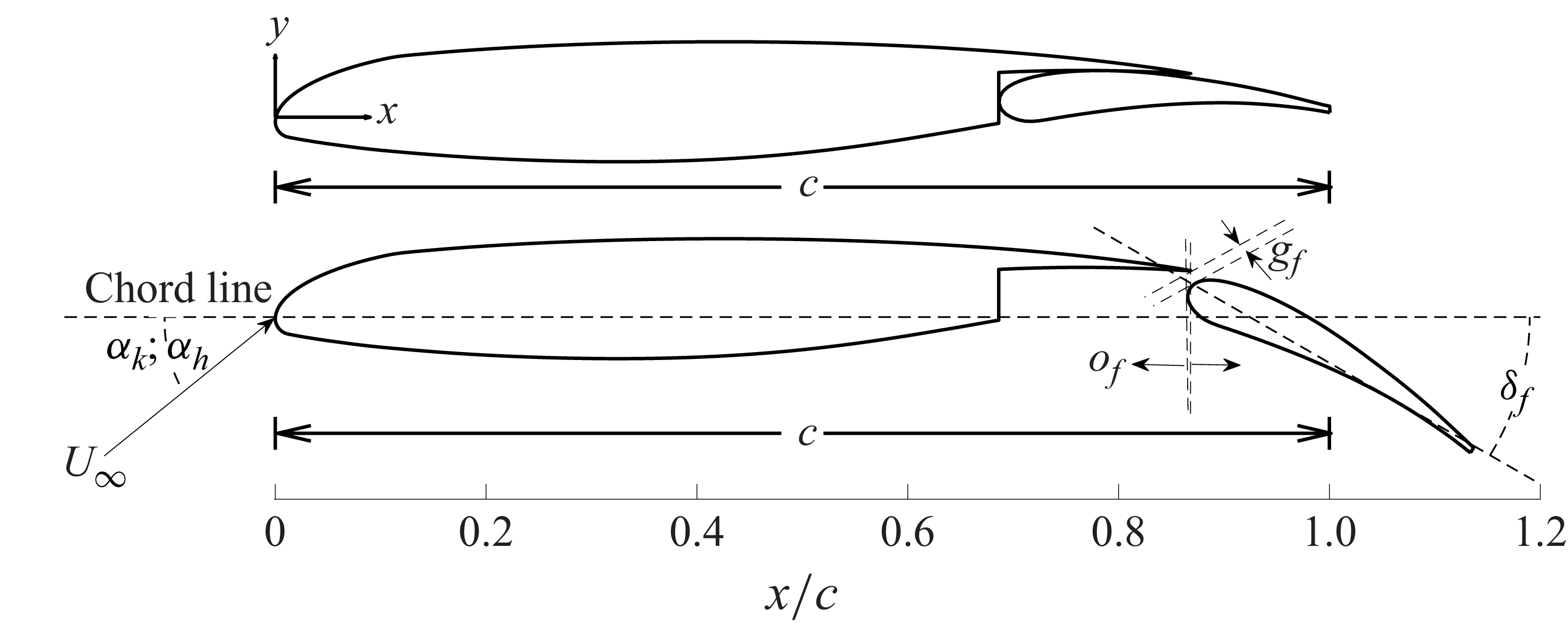
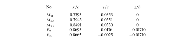
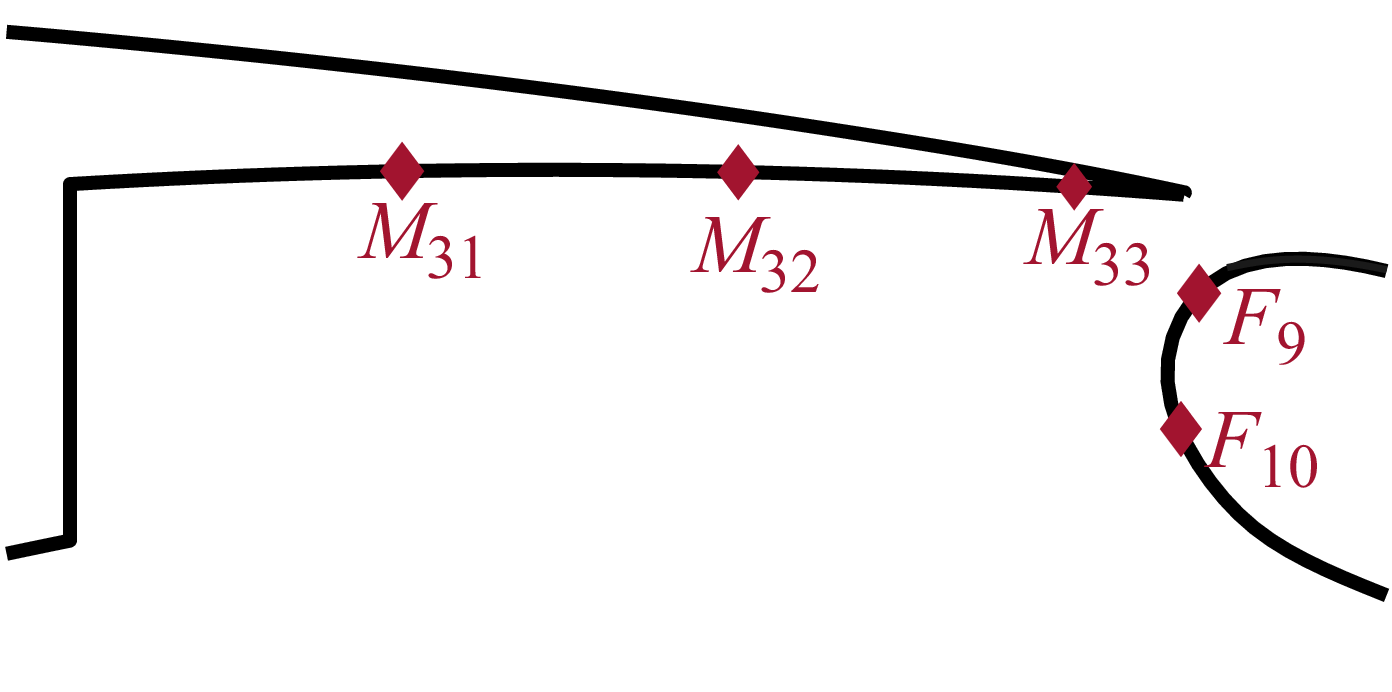


 ω

 U∞=55
 ⟨u⟩/U∞
 ⟨v⟩/U∞
 ⟨ωz⟩⋅c/U∞
 αh=0∘
 αh=3∘
 αh=6∘

 U∞=55
 ⟨u′2⟩/U∞2
 ⟨v′2⟩/U∞2
 ⟨u′v′⟩/U∞2
 αh=0∘
 αh=3∘
 αh=6∘
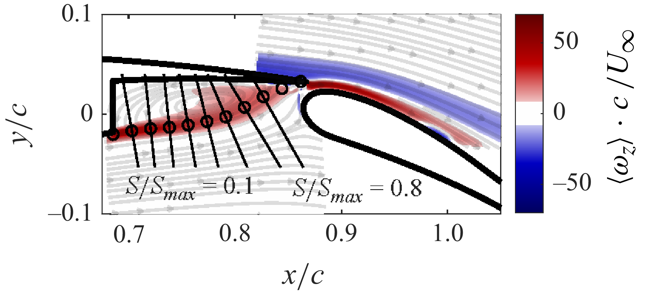
 αh=6∘


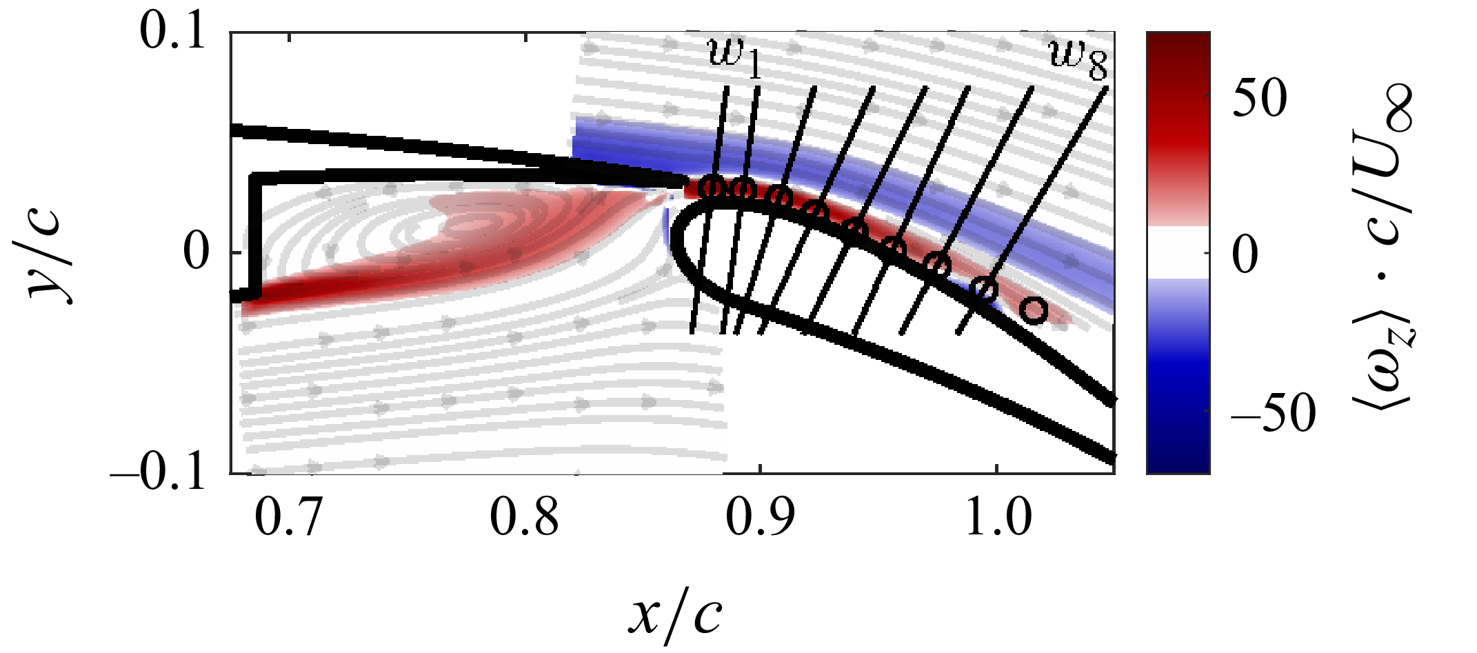


 αh=0∘
 U∞=55
 Ru′,p′
 Rv′,p′
 Ru′,p′
 Rv′,p′
 F9
 Ru′,p′
 Rv′,p′
 F10
 Ru′,p
 Rv′,p′
 M32
 Ru′,p
 Rv′,p′
 M33

 U∞=55
 y/c
 ⟨ωz⟩⋅c/U∞
 ⟨u⟩/U∞

 U∞=55
 ⟨u′2⟩/U∞2
 ⟨v′2⟩/U∞2
 ⟨u′v′⟩/U∞2
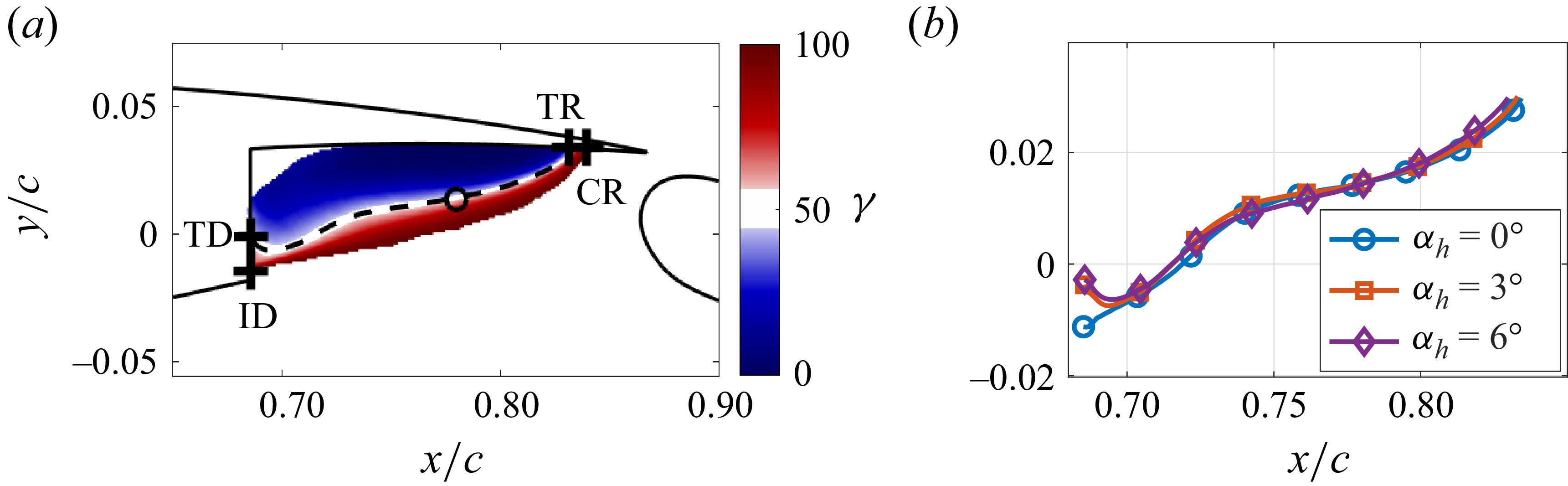
 U∞=55
 (γ)
 αh=3∘
 γ>99%
 ⟨u⟩=0
 (⟨u⟩=0)
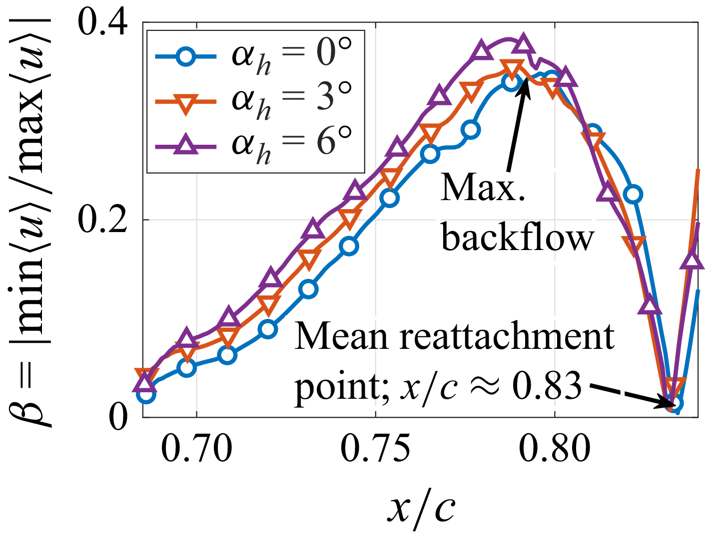
 β=|min⟨u⟩/max⟨u⟩|

 ⟨U⟩/U∞
 αh=0∘
 U∞=55

 αh=0∘
 U∞=55

 max(ωz)
 αk=3∘
 U∞=55

 αk=3∘
 U∞=55

 αh=0∘
 U∞=55
 x/c≈0.8;y/c≈0
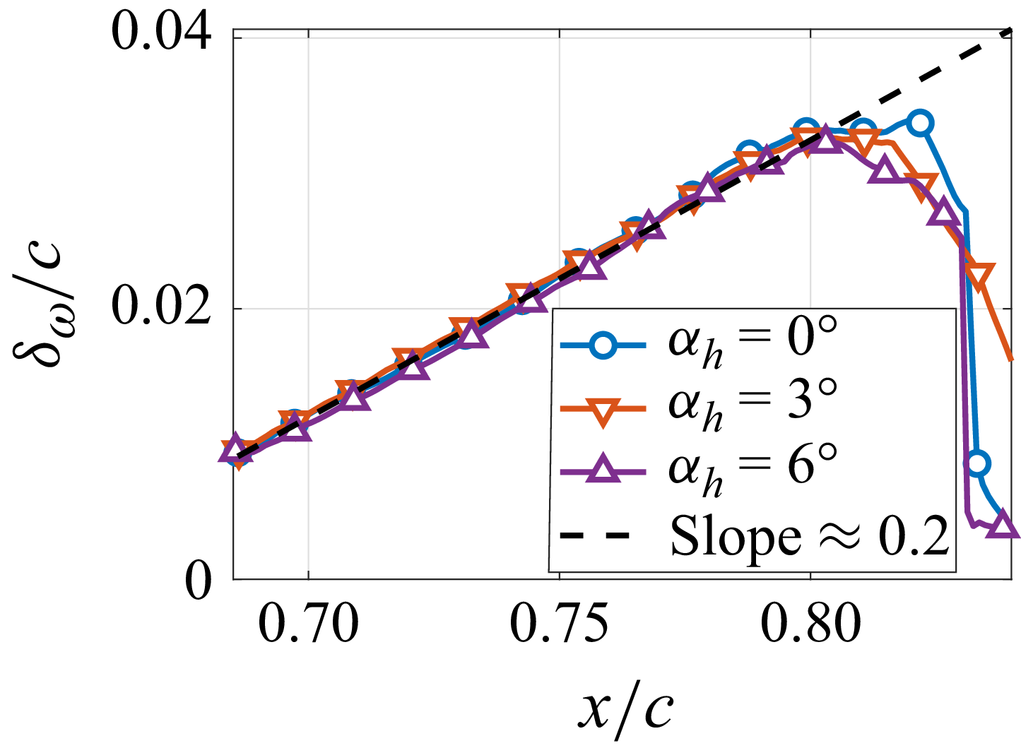
 δω
 δω=(U∞−⟨u⟩min)/max|⟨du/dy⟩|
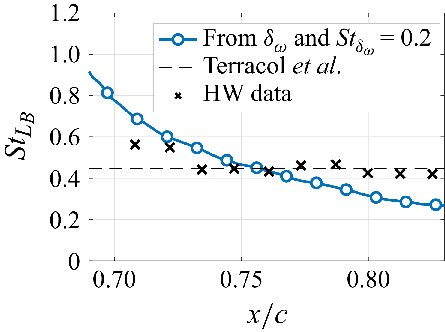
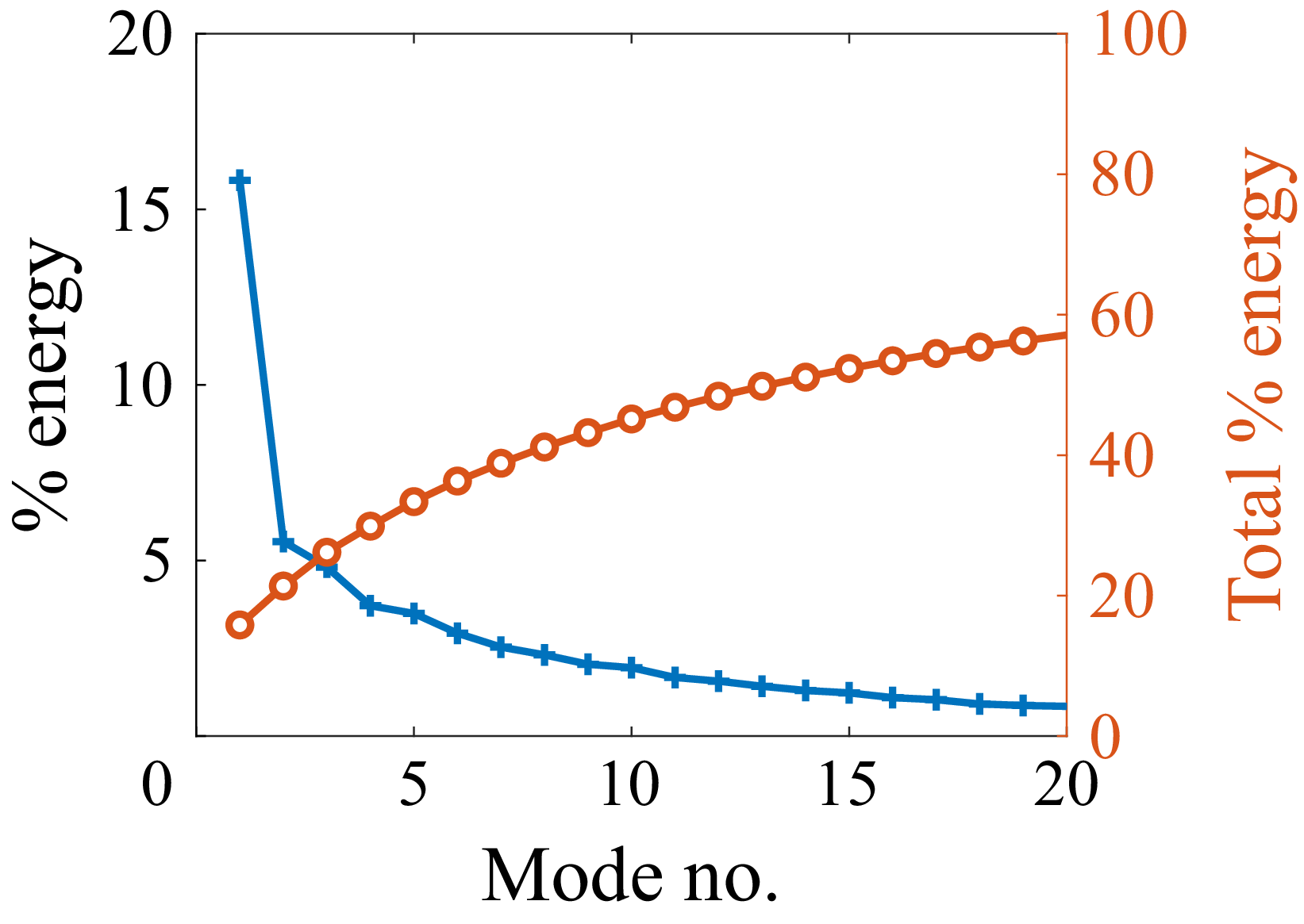
 αh=0∘
 U∞=55

 αh=0∘
 U∞=55
 Ψiv

 αh=0∘
 U∞=55

 αh=0∘
 U∞=55
 Ψiv
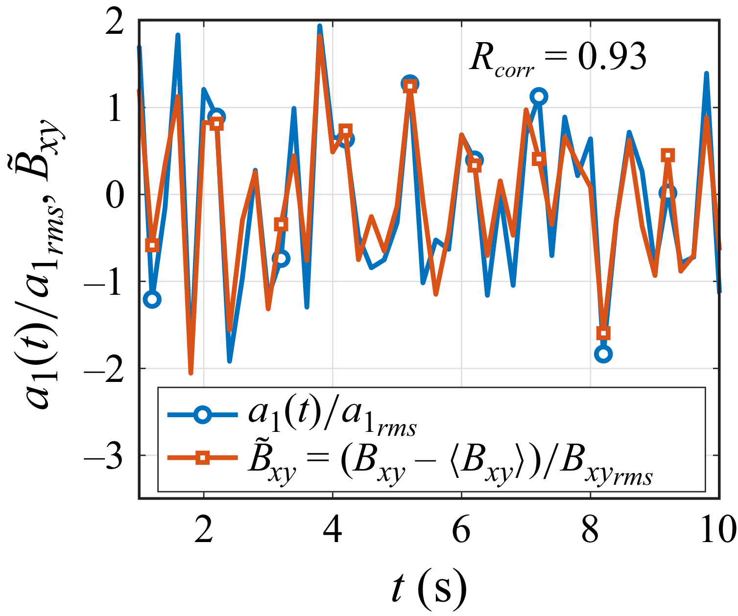
 a1(t)
 Bxy(t)

 x-
 yk=10/c
 y-
 xk=10/c
 x
 y-
 (xk=10,yk=10)/c


 (⟨u⟩−U∞)/U∞
 (u~a1−U∞)/U∞=0.3
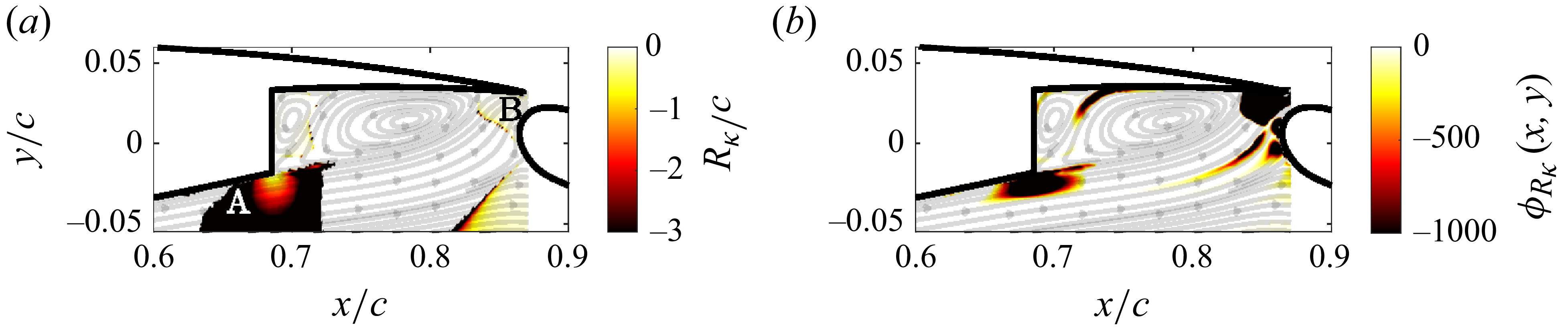

 δ/Rκ
 λT/Rκ⋅UeλT/νtot=250

 Q=2×10⁶
 −2
 ωx

 M33
 x/c=0.8491
 M32
 x/c=0.7943
 Rsum
 T1
 T2
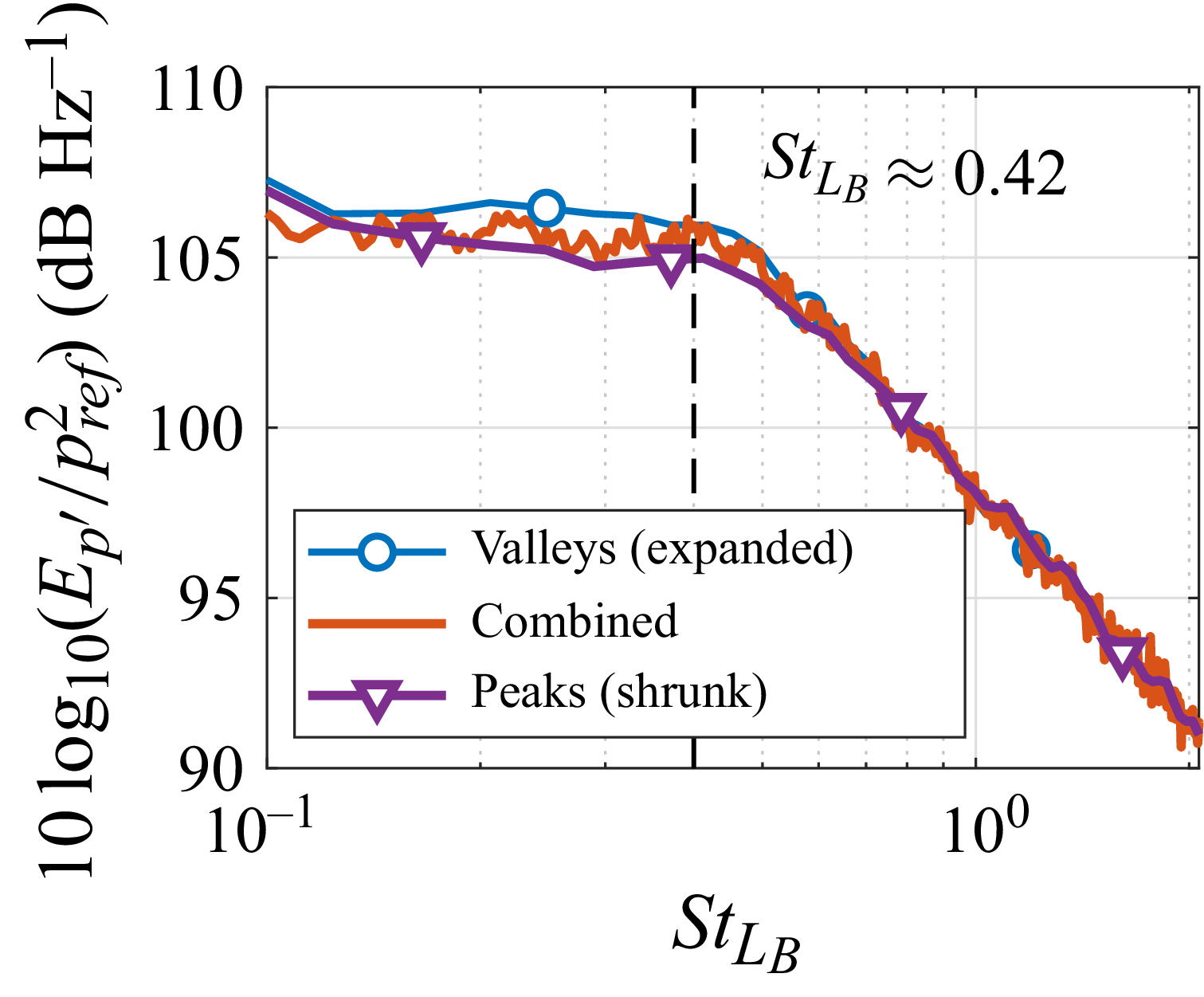
 M33


 Open access

