



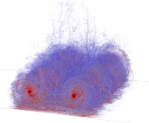



1. Introduction
We here consider a two-vortex system (2VS), i.e. a pair of counter-rotating vortices as is typical of the wake produced by a wing, and assume that the wake rollup happened away from the ground; thus out of ground effect (OGE). When the Reynolds number is high, the subject also relates to the wake produced by aircraft. The wake-vortex-encounter related hazard then considers the effect that such a wake system could have on a follower aircraft. It is most critical when at low altitude, and is used to define the separations to be applied between landing aircraft; also taking into account the wake vortex's further interaction with the ground (De Visscher, Winckelmans & Treve Reference De Visscher, Winckelmans and Treve2016). Much effort has been devoted to a better understanding of wake vortex physics (see reviews by Spalart (Reference Spalart1998), Gerz, Holzapfel & Darracq (Reference Gerz, Holzäpfel and Darracq2002) and Coustols, Jacquin & Schrauf (Reference Coustols, Jacquin and Schrauf2006)), also to support the establishment of separation standards without compromising safety; such as in RECAT-EU (Rooseleer et al. Reference Rooseleer, Treve, De Visscher and Graham2016). Better understanding, and also modelling, of the interaction of high-Reynolds-number wake vortices with the ground thus constitutes a subject of significant interest: in itself as a problem involving complex physics, and also in support of air traffic safety.
The presence of the ground impacts both the trajectory and the decay of the vortices (Doligalski, Smith & Walker Reference Doligalski, Smith and Walker1994); as was also measured experimentally in Lidar measurement campaigns (Holzäpfel & Steen Reference Holzäpfel and Steen2007; De Visscher et al. Reference De Visscher, Winckelmans and Treve2016). Their descent is first altered by the impermeability condition at the ground: this early phase is essentially inviscid and the vortices follow a hyperbolic trajectory (Lamb Reference Lamb1932); this is the near ground effect (NGE) phase. As the vortices descend farther, they interact with the opposite sign secondary vorticity from the separating boundary layers, which eventually leads to the ‘rebound’ of the vortices, i.e. an upward motion as first explained by Harvey & Perry (Reference Harvey and Perry1971). This phase is the in ground effect (IGE) phase. Two-dimensional (2-D) simulations at various Reynolds numbers were already reported by Zheng & Ash (Reference Zheng and Ash1996), Corjon & Poinsot (Reference Corjon and Poinsot1997), Proctor et al. (Reference Proctor, Hinton, Han, Schowalter and Lin1997) and Türk, Coors & Jacob (Reference Türk, Coors and Jacob1999).
It is the strong interaction between the secondary vorticity and the primary vortices that is responsible for the increased decay rate of those vortices when IGE. At low Reynolds numbers, as  $Re_\varGamma \simeq 2\unicode{x2013}5\times 10^3$ typical of water tank experiments (
 $Re_\varGamma = \varGamma _0/\nu$ based on the initial vortex circulation
 $\varGamma _0$ and the fluid kinematic viscosity
 $\nu$), the main mechanism is a short wavelength instability, similar to the elliptic instability (Widnall, Bliss & Tsai Reference Widnall, Bliss and Tsai1974), that develops on the secondary vortices; as also observed experimentally by Harris & Williamson (Reference Harris and Williamson2012) and numerically by Luton & Ragab (Reference Luton and Ragab1997). At even lower Reynolds numbers, the dominant instability mechanism is similar to that of a long-wave Crow-type instability (Crow Reference Crow1970) whereas the elliptic instability becomes the most unstable mode as
 $Re_\varGamma$ increases, as was shown by Leweke, Le Dizès & Williamson (Reference Leweke, Le Dizès and Williamson2016).
The presence of a cross-flow can also modify the rebound and decay of vortices IGE, as both vortices no longer exhibit symmetrical behaviours (Doligalski et al. Reference Doligalski, Smith and Walker1994). This was investigated by Stephan, Holzäpfel & Misaka (Reference Stephan, Holzäpfel and Misaka2013), Holzäpfel, Tchipev & Stephan (Reference Holzäpfel, Tchipev and Stephan2016) and Bricteux et al. (Reference Bricteux, Duponcheel, De Visscher and Winckelmans2016), using fine resolution wall-resolved large-eddy simulation (LES) at  $Re_\varGamma = 2\times 10^4$, and where analytical vortices were added to a turbulent crosswind (itself obtained using a presimulation). Various crosswind intensities were investigated. In Stephan et al. (Reference Stephan, Holzäpfel and Misaka2013) and Holzäpfel et al. (Reference Holzäpfel, Tchipev and Stephan2016) the impact of a headwind was also studied.
Beside the transport by the wind and the induced asymmetry, the simulations of vortices IGE at  $Re_\varGamma = 2\times 10^4$ and in a turbulent crosswind (Stephan et al. Reference Stephan, Holzäpfel and Misaka2013; Bricteux et al. Reference Bricteux, Duponcheel, De Visscher and Winckelmans2016; Holzäpfel et al. Reference Holzäpfel, Tchipev and Stephan2016) also showed that the wind turbulence strongly affects the boundary layers developing on the wall, their separation and their interaction with the primary vortices. The separated vorticity is seen to be directly three-dimensional (3-D), and thus it does not need to go through an elliptic instability to transition to turbulence. This alteration of the separated secondary vorticity therefore also influences the primary vortex trajectories and decay. In Stephan et al. (Reference Stephan, Holzäpfel and Misaka2013) they proposed that the boundary layers are mainly perturbed by pre-existing turbulent structures of the wind. In Bricteux et al. (Reference Bricteux, Duponcheel, De Visscher and Winckelmans2016) they showed that the perturbations are mostly linked to turbulent structures of the wind that are altered and stretched by the primary vortices during their descent, and then interact with the boundary layers. Finally, it is also worth mentioning that Proctor & Han (Reference Proctor and Han1999) and Proctor, Hamilton & Han (Reference Proctor, Hamilton and Han2000) also simulated wake vortices IGE at high Reynolds numbers in turbulent atmospheres, and reported on global transport and decay; yet this was done using coarse resolution wall-modelled LES. As the boundary layers are not resolved, such LES do not capture in much detail the interactions between the vortices, the wind turbulence and the ground.
We note that many of the available simulations were initialised using analytical model vortices that were added to a realistic background turbulent field: atmospheric turbulence (Proctor & Han Reference Proctor and Han1999; Proctor et al. Reference Proctor, Hamilton and Han2000), or a turbulent boundary layer obtained using a presimulation and representing a turbulent wind (Stephan et al. Reference Stephan, Holzäpfel and Misaka2013; Bricteux et al. Reference Bricteux, Duponcheel, De Visscher and Winckelmans2016; Holzäpfel et al. Reference Holzäpfel, Tchipev and Stephan2016).
In Stephan, Holzäpfel & Misaka (Reference Stephan, Holzäpfel and Misaka2014), the vortex pair was generated using a Reynolds-averaged Navier–Stokes (RANS) simulation of the flow past the aircraft, and an LES of wake rollup, resulting in a vortex pair with realistic turbulent content. The two methods were coupled using some transition function, so that the 3-D RANS flow field serves as an initial ‘forcing term’ of the filtered Navier–Stokes equations for the LES. The methodology was also used in Misaka, Holzäpfel & Gerz (Reference Misaka, Holzäpfel and Gerz2015). It was further developed and improved in Stephan et al. (Reference Stephan, Rohlmann, Holzäpfel and Rudnik2019) by translating the turbulent kinetic energy (TKE) of the RANS simulation field into resolved white noise turbulence for the LES. This then constitutes a quite advanced method to generate aircraft wake vortices whose velocity field and larger-scale turbulence are governed by the flow around the complex aircraft geometry, and also in landing configuration.
When adding some white noise perturbation to trigger instabilities, this results in an artificial time for the development of the instabilities. When model vortices are added to some turbulence OGE, they interact with it, which eventually leads to turbulent vortices with some circulation decay rate, but too late (see, e.g. De Visscher, Bricteux & Winckelmans (Reference De Visscher, Bricteux and Winckelmans2013a)). And when model vortices are added to a turbulent cross-flow at a low release altitude of  $h_0\simeq b_0$ as in Bricteux et al. (Reference Bricteux, Duponcheel, De Visscher and Winckelmans2016) (
 $b_0$ being the initial spacing between the centres of the vortices), they do not have time to strongly interact with that turbulence while descending; they mainly interact with the ground, producing boundary layers, and strong turbulence is only generated later when the secondary vorticity from the separating boundary layers goes 3-D and further interacts with the primary vortices.
In order to better understand the physics, it thus appears important to also properly capture the turbulence of the 2-VS itself; also to have a better initial condition for IGE simulations. The present paper aims to address those points by: (i) considering a vortex pair that is evolved in weak turbulence and reaches its own fully developed ‘turbulent equilibrium state’ (which we call a T-2VS); and (ii) study the interaction of this fully developed T-2VS with the ground, at a high Reynolds number and using a wall-resolved simulation.
We stress that the second part of the present study does not consider any added complexity, such as a background turbulent wind, or the ground roughness, or an initial inclination of the vortex pair relatively to the ground with associated end effects (as in Stephan et al. (Reference Stephan, Holzäpfel and Misaka2014)), or the details of a vortex system generated directly behind an aircraft when the rollup takes place near the ground (as in Stephan et al. (Reference Stephan, Rohlmann, Holzäpfel and Rudnik2019)). The aim is to provide a detailed analysis of the interaction of a fully developed T-2VS with a smooth ground, and when the T-2VS is parallel to the ground.
Our wall-resolved simulation is conducted at  $Re_\varGamma = 2 \times 10^5$: this is
 $10 \times$ higher than in the previous wall-resolved simulations of Bricteux et al. (Reference Bricteux, Duponcheel, De Visscher and Winckelmans2016), Stephan et al. (Reference Stephan, Holzäpfel and Misaka2013) and Holzäpfel et al. (Reference Holzäpfel, Tchipev and Stephan2016) and it will hence allow us to better capture the high-Reynolds-number behaviour. The release height of the T-2VS is also taken twice higher here, using
 $h_0=2\,b_0$; this ensures a physically correct approach to the ground, with a well-captured NGE phase of the T-2VS, before going into the IGE phase with the strong interaction of the T-2VS with the ground.
The paper is organised as follows: § 2 briefly reminds the reader of analytical wake vortex models widely used; as initial conditions or for analysis purposes. Section 3 details how the T-2VS at equilibrium is obtained and it then describes its main characteristics. A sensitivity analysis is also conducted, by varying the initial vortex models and perturbation field. Section 4 presents the wall-resolved LES of the T-2VS when further put in a NGE situation: we first briefly present the numerics and how the initial condition is set using the results of the T-2VS that was obtained OGE. The behaviour of the vortex pair when evolving from NGE to IGE is then studied in detail: in terms of flow topology, global diagnostics and detailed circulation distributions. The results are also usefully compared with the case where the initial condition consists of non-turbulent vortices (i.e. analytical model vortices) with some added white noise perturbation.
2. Recall of some analytical wake vortex models
The vortex centroids of a 2VS are separated by  $b_0$, which is related to the wingspan
 $b_w$ and to the span loading distribution. Initially, the vortices have a total circulation
 $\varGamma _0$ and
 $-\varGamma _0$, respectively. They sink under their mutual influence, at the velocity
 $W_0 = \varGamma _0/(2{\rm \pi} b_0)$ when OGE. This also defines the characteristic time
 $t_0 = b_0/W_0$: the time it takes for the 2VS to descend one
 $b_0$.
For systems with vortices of small core size, as here, the vorticity field of each vortex is essentially axisymmetric. Each vortex is then characterised by its mean circulation distribution,  $\varGamma (r)$: the amount of vorticity contained in a disk of radius
 $r$ centred on the vortex. The vortex-induced velocity is then
 $u_\theta ( r ) = \varGamma ( r )/(2{\rm \pi} r)$. The aforementioned simulations of wake vortices were performed using, as initial conditions, either an analytical model for
 $\varGamma (r)$ or the result of a rollup simulation using RANS; and perturbed to excite instabilities.
A simple model often used for wake vortices after rollup in the aircraft community is the Burnham–Hallock (BH) model (Burnham & Hallock Reference Burnham and Hallock1982)
 \begin{equation} \frac{\varGamma( r )}{\varGamma_0}= \frac{r^2}{(r^2+r_c^2)} \end{equation}
with  $r_c$ the ‘effective core radius’ (defined as the radius of maximum induced velocity). The induced velocity is thus
 \begin{equation} u_\theta( r) = \frac{\varGamma_0}{2{\rm \pi}}\,\frac{r}{(r^2+r_c^2)}. \end{equation}
Note that it also corresponds to the Rosenhead–Moore regularisation of a point vortex, where the  $1/r$ singularity of the velocity field is replaced by
 $r/(r^2+r_c^2)$.
Another model is the Gaussian model, also called the Lamb–Oseen (LO) model
 \begin{equation} \frac{\varGamma( r )}{\varGamma_0} = 1 - \exp\left({-}a \left(\frac{r}{r_c}\right)^2\right) \quad {\rm with}\ a = 1.2564 . \end{equation}
We note that the models above are all regular: the induced velocity is zero at  $r=0$ and is linear for small
 $r$; hence the circulation distribution is quadratic for small
 $r$. Those models have been used in studies of wake vortices interacting with the ground, also in the presence of a turbulent wind: as in Holzäpfel et al. (Reference Holzäpfel, Tchipev and Stephan2016) using the LO model and in Bricteux et al. (Reference Bricteux, Duponcheel, De Visscher and Winckelmans2016) using the BH model.
Yet, when considering a better description of the circulation distribution  $\varGamma (r)$ of vortices in a realistic turbulent vortex pair, two-scale models are required, with a Gaussian-like ‘inner region’ displaying a rapid growth and scaling with
 $r_c$, and an ‘outer region’ displaying a slow growth and scaling with
 $b_0$ (or
 $b_w$). Such models include those by Fabre & Jacquin (Reference Fabre and Jacquin2004) or that by Proctor (Reference Proctor1998) and further modifications thereof; among which being the improved version of Proctor et al. (Reference Proctor, Ahmad, Switzer and Duparcmeur2010). The inner and outer parts of the improved model (P model) read
 \begin{equation} \left.\begin{gathered} \frac{\varGamma( r )}{\varGamma_0}= C\left(1 - \exp\left({-}a \left(\frac{r}{r_c}\right)^2\right) \right) \quad {\rm for} \ 0\leq r \leq \alpha\, r_c ,\\ \frac{\varGamma( r )}{\varGamma_0} = 1 - \exp\left(-\beta \left(\frac{r}{b_w}\right)^{q}\right) \quad {\rm for} \ r \geq \alpha r_c. \end{gathered}\right\} \end{equation}
The proposed calibrated values are  $q\simeq 0.75$,
 $\beta \simeq 10.0$ and
 $\alpha \simeq 1.4$. Note that the most important parameter is the exponent
 $q$. The parameter
 $\beta$ is found to depend on the initial vorticity distribution in the near wake. As for
 $\alpha$, it is only a convenient parameter used to define where one switches from the model for the inner part to the model for the outer part. Once those parameters are fixed, the
 $C$ coefficient is determined by enforcing the continuity at
 $\alpha r_c$ (yet the model is not differentiable there). The model of (2.4) is clearly over-simplistic as a Gaussian behaviour (which corresponds to diffusion with a constant diffusivity coefficient) cannot be valid beyond
 $r_c$. Using a value of
 $\alpha < 1$ would also not be appropriate as the outer scaling function cannot already start at a radius below
 $r_c$.
A mathematically smoother version of the model (called the PW model) was proposed by Winckelmans, using a smooth blending between the inner and outer functions (see de Bruin & Winckelmans (Reference de Bruin and Winckelmans2005) and De Visscher et al. (Reference De Visscher, Winckelmans, Lonfils, Bricteux, Duponcheel and Bourgeois2010))
 \begin{equation} \frac{\varGamma( r )}{\varGamma_0}= 1 - \exp\left(- \frac{a_i \left(\dfrac{r}{r_c}\right)^2}{\left[1 + \left(\dfrac{a_i \left(\dfrac{r}{r_c}\right)^2}{\beta_o\left(\dfrac{r}{b_0}\right)^{3/4}}\right)^p\right]^{1/p} } \right) . \end{equation}
That model recovers the inner and outer behaviours of (2.4). Being obtained using a smooth blending, it does not suffer from the issue of where to switch from the inner model to the outer model. The blending also ensures that the Gaussian behaviour is only for  $r$ smaller than
 $r_c$. Note that we here elected to use
 $b_0$ instead of
 $b_w$ as the reference outer scale; hence
 $\beta _o= ({b_0}/{b_w})^{3/4}\beta$ (for a wing with elliptical loading,
 ${b_0}/{b_w}={{\rm \pi} }/{4}$ and thus
 $\beta _o \simeq 8.34$ when
 $\beta =10.0$). The
 $p$ exponent is used to adjust the amplitude of the maximum induced velocity,
 $u_\theta (r_c)$, for any fixed
 $r_c$; typical values are in the range
 $p=3\unicode{x2013} 5$. The value of
 $a_i$ is then determined by imposing that the maximum induced velocity occurs at exactly
 $r=r_c$. For vortices with
 $r_c/b_0=0.050$ as considered here, and using
 $\beta _o=8.34$ and
 $p=4$, one obtains
 $a_i=0.802$.
The circulation and induced velocity profiles of those vortex models are provided in figure 1. We see that the BH single-scale model appears as a good choice for approximating the more physical two-scale models; which helps support its wide use in the aircraft wakes community. However, the  $\varGamma ( r )$ values of the BH model are still too high in the region from
 ${\simeq }2 r_c$ to
 ${\simeq }5r_c$.
Circulation (a) and induced velocity (b) profiles for various wake vortex models: single scale models, BH (thin solid) and LO (thin dash); two-scale models for the case  $r_c/b_0= 0.050$,
 $P$ (dash) and PW (solid).

3. Turbulent two-vortex system at equilibrium
The models presented in § 2 only describe the mean vortex; they do not provide the fluctuations. In reality, the wake formed behind a wing at high Reynolds number quickly develops its own turbulence while it rolls up, resulting in a turbulent 2VS with significant turbulent structures within the Rankine oval, and near it. As we will see, the turbulence of such T-2VS will also play an important role when it further interacts with the ground. Obtaining a realistic, fully developed, T-2VS is thus of importance, not only for better characterising the circulation distribution  $\varGamma (r)$ and associated turbulence of fully developed wakes, but also when using it as an initial condition for the investigation of those wakes interacting with the ground. This is even more important when one considers interactions without added turbulent wind, as will be the case here. The next section presents the methodology used here to obtain a T-2VS.
3.1. Numerical set-up
The simulations are performed in a periodic box of volume  $V_e = L_e^3 = (4b_0)^3$ and using a pseudospectral code with phase shift dealiasing (Canuto et al. Reference Canuto, Yousuff Hussaini, Quarteroni and Zang2006). First, a forced homogeneous isotropic turbulence (HIT) simulation is performed to obtain a converged turbulence field. Then, a model 2VS is added to this precursor field. We consider vortices with a core size of
 $r_c/b_0 = 0.050$, as in Bricteux et al. (Reference Bricteux, Duponcheel, De Visscher and Winckelmans2016), and we first use the BH model for the initial circulation distribution within each vortex. The grid size used for that pseudospectral LES is
 $256^3$ (thus a grid spacing
 $\varDelta =b_0/64$); thanks to the spectral properties of the code, this is equivalent to a
 $512^3$ simulation when using our fourth-order finite difference code in § 4.
We do not claim that the dynamics of all small scales inside the vortex cores are here fully resolved; that would require a finer grid, and likely also running the simulation in direct numerical simulation mode: something that would be extremely costly at the high Reynolds number considered here. The present study focuses on obtaining a turbulent state of two counter-rotating vortices, and using LES (thus necessarily under-resolved for the turbulence, with subgrid scales (SGSs) not captured). The turbulence will be obtained for radii greater than  $r_c$ and up to roughly
 $b_0/2$, where the turbulent vorticity of one vortex will then strongly interact with that of the other one, making the total circulation of each vortex slowly decrease. The turbulent part of the vortices is the part that we focus on.
We also stress that the Crow instability, that has a slow growth rate, and which is maximum for the wavelength  $\lambda _x\simeq 8 b_0$, will not develop here; this is on purpose since we aim to obtain a fully developed T-2VS that, in reality, would form within less than one
 $t_0$ behind a wing, through the rollup of the near wake; in such a short time, the Crow instability does not have time to develop. We refer to De Visscher et al. (Reference De Visscher, Bricteux and Winckelmans2013a) for a previous investigation performed using a 2VS subjected to various levels of atmospheric turbulence and stratification, with a periodic box of
 $(8b_0)^3$ and using the same pseudospectral LES code, with the same core size and grid resolution, and using BH vortices for the initial condition. Those simulations focused on capturing the evolution of the wake up to its complete demise, and also on developing a simplified operational model. Simulations of wake demise due to the Crow instability in atmospheric turbulence, and also combined with stratification effects, were also presented in Misaka et al. (Reference Misaka, Holzäpfel and Gerz2015).
As to the energy dissipation rate,  $\epsilon _0$ (units of
 $\textrm {{m}}^2\ \textrm {{s}}^{-3}$), of the HIT perturbation field used here, it must be characterised relatively to the 2VS global length and velocity scales; hence using the dimensionless
 $\epsilon _0^\ast = (\epsilon _0 b_0)/W_0^3$. We obtain that
 $\epsilon _0^\ast = 2.42 \times 10^{-4}$; this is indeed a case of very weak turbulence.
The initial kinetic energy of the mean cross-flow velocity field, noted  $(V,W)$, is
 \begin{equation} E_{2D,0} = \int_{S_e} \frac{\left(V^2 + W^2\right)}{2}\,{\rm d}S, \end{equation}
where  $S_e = 4b_0 \times 4b_0$. Its units are
 $\textrm {{m}}^4\ \textrm {{s}}^{-2}$. We obtain, in dimensionless form,
 $E_{2D,0}/(W_0b_0)^2 = 15.38$. The kinetic energy of the total initial flow field (HIT field added to the BH-2VS, thus with
 $(u,v,w)=(u', V+v', W+w')$) is, after longitudinally averaging in order to compare with
 $E_{2D,0}$,
 \begin{equation} E_0 = \frac{1}{L_e} \int_{V_e} \frac{\left(u^2 + v^2 + w^2\right)}{2} \,{\rm d}V = E_{2D,0} + E_{f,0}. \end{equation}
We obtain  $E_0/(W_0b_0)^2 = 15.44$. Thus, the kinetic energy associated with the added fluctuations amount to only approximately 0.4 % of
 $E_0$. Nevertheless, and as we will see later, this very weak HIT field added to the 2VS will suffice to lead, after a long transient, to a fully developed turbulent 2VS.
For completeness, we also report the energy of the same BH-2VS when considered in unbounded space. Since the core size is small, this energy can be estimated accurately by using the formulae developed in de Bruin & Winckelmans (Reference de Bruin and Winckelmans2005),
 \begin{equation} E_{2D,0}^\infty = \frac{\varGamma_0^2}{2{\rm \pi}}\left(\log\left(\frac{b_0}{r_c}\right)-C\right) \quad\Rightarrow\quad \frac{E_{2D,0}^\infty}{(W_0b_0)^2} = 2{\rm \pi}\left(\log\left(\frac{b_0}{r_c}\right)-C\right) , \end{equation}
where  $C=\frac 12$ when using BH vortices (note that
 $C=-0.05617$ when using LO vortices). We obtain
 $E_{2D,0}^\infty /(W_0b_0)^2 = 15.68$. Thus only a 2 % difference with the value for the 2VS put in a periodic domain; comforting us that the size
 $L_e = 4 b_0$ of the periodic computational domain used here is large enough for the purpose of our study. The descent velocity
 $W_0$ of the 2VS in the periodic domain is also measured and compared with that in an unbounded domain; it is a bit slower, by roughly 1.3 %.
Finally, we also note that the present BH-2VS has roughly the same energy as that of the near wake vortex sheet that would emanate from a wing with an elliptical loading; indeed, the lifting line theory gives  $E_{2D,{ellip}}=\varGamma _0^2\,({{\rm \pi} }/{8})$, and thus
 $E_{2D,{ellip}}/(W_0b_0)^2 = {{\rm \pi} ^3}/{2} = 15.50$. As to the LO-2VS with the same
 $r_c/b_0=0.050$, its energy is significantly higher:
 $19.18$, which would correspond to a wing that is significantly more outboard loaded than one with elliptical loading. To have a LO-2VS that has the same energy as that of the present BH-2VS would require us to use
 $r_c/b_0\simeq 0.087$.
3.2. Results: transient and characterisation of the obtained T-2VS
The results obtained using a 2VS with BH model vortices and added very weak HIT (referred to as the ‘baseline Case 0’) are analysed in this section. Although the added HIT field is very weak relative to the 2VS, we see that their combination leads, after a long transient, to a ‘2VS at turbulent equilibrium’ (i.e. T-2VS) where all the wavenumbers are energised. This is illustrated by the time evolution of the kinetic energy (see figure 2 with the modal energies, mean 2-D flow energy and total flow energy), and of the total energy dissipation rate,  ${\mathcal {E}} = -{\textrm {d}E}/{\textrm {d}t}$ with units
 $\textrm {{m}}^4\ \textrm {{s}}^{-3}$ (see Case 0 in figure 3).
Evolution of the kinetic energy for the baseline Case 0. (a) Longitudinal modal energy: mean flow (thick solid), mode  $\lambda =4b_0$ (solid) and next 31 modes (thin solid) down to
 $\lambda =0.125b_0$. (b) Total energy
 $E$ (solid) and mean flow energy
 $E_{2D}$ (dashed).

Evolution of the dimensionless energy dissipation rate. (a) Baseline BH-2VS (Case 0, solid), PW-2VS (Case 1, dashed–dotted) and LO-2VS (Case 2, dashed), all with very weak HIT. (b) The BH-2VS with very weak HIT (Case 0, solid) and with HIT of  $10 \times$ higher dissipation rate (Case 3, dashed).

The present simulation must be understood as an artificial transient process, using a 2VS made of analytical model vortices and a weak HIT field as sole added perturbation, to finally obtain, using a time-developing simulation, a turbulent equilibrium state of the 2VS. As the perturbation is here very weak, it takes a long transient to obtain the T-2VS, see figures 2 and 3. If we examine the saturation of the high-wavenumber modes, we see that the equilibrium is reached at approximately  $t/t_0\simeq 4.5$. Examining the time evolution of the energy, we see that the energy of the mean flow decreases while the total energy is still essentially conserved until
 $t/t_0\simeq 3.5$; showing that a significant amount of energy has been transferred from the mean flow to fluctuations, and so far in an essentially inviscid way. Later on, we see that the total energy also decreases, and with essentially the same rate as that of the mean flow, meaning that, from now on, the kinetic energy associated with the fluctuations is well established relative to the mean flow. The 2VS has indeed reached a statistical equilibrium around
 $t/t_0\simeq 4.5$: a state where the mean flow and the turbulence are both established and are continuously interacting with each other, and where the dissipation rate also decreases.
We stress that the present process used to obtain a T-2VS takes much more time than what happens for a real wake developing behind a wing, or aircraft in cruise, where the T-2VS in the wake would be reached within the distance required to fully complete the wake rollup, and which is typically close to  $U_\infty t_0$ (here
 $U_\infty$ is the flight velocity,
 $x$ is the distance to the wing/aircraft and
 $x/U_\infty$ replaces the time
 $t$ of a time-developing simulation). For an aircraft in landing configuration, with the flaps deflected, the near wake is much more complex, and it can take a distance of
 $\simeq 2U_\infty t_0$ to fully complete the rollup. Significant turbulence is then also present in the near wake vorticity (e.g. from the boundary layers on the aircraft surfaces and the engine jets). Furthermore, instabilities develop during the wake rollup itself, creating additional turbulence. The dissipation rate of the kinetic energy is typically at its highest level in the near wake behind the aircraft, and it decreases downstream as the wake rolls up. The total energy (mean flow and fluctuations) integrated in each downstream cross-plane (i.e. Treftz plane) is
 $E(x)$ (also with units
 $\textrm {{m}}^4\ \textrm {{s}}^{-2}$), and the dissipation rate of that energy,
 ${\mathcal {E}}= -U_\infty \,{\textrm {d}E}/{\textrm {d}\kern0.7pt x}$ (since
 ${\textrm {d}\kern0.7pt x}/{U_\infty }$ replaces
 $\textrm {d}t$), is here a decreasing function of
 $x$. When the equilibrium is obtained after complete rollup, the dissipation rate is significantly lower than that in the near wake, and it is determined by the turbulent equilibrium itself. Energy is constantly being transferred from the large and mostly 2-D scales of the flow to azimuthal medium scales, and down to fine scales where the dissipation occurs.
We recall that a turbulent equilibrium is a state where the mean flow and the fluctuations are both well established, and where the dissipation rate decreases, and that this state does not depend on the path followed to obtain it. For instance, the fully developed turbulent jet is also a flow in equilibrium; another example is the fully developed turbulent wake behind a body with pure drag. In such flows, and also the present one, there is production of TKE by the interaction of the mean flow and the turbulence, and the dissipation rate  ${\mathcal {E}}(x)$ decreases in
 $x$ while the mean flow velocity profile remains self-similar. We hence speculate that the T-2VS obtained after complete rollup of the wake behind a wing at high Reynolds number, or aircraft, could be similar to the T-2VS obtained here. The core size
 $r_c$ would, however, be different, and likely smaller than that of the present simulation.
We also see that a mode of wavelength  $\lambda =4b_0$ develops in our simulation and that it does not increase after
 $t\simeq 4 t_0$; it remains at a low level, and it even decreases after
 $t= 5 t_0$ – this mode corresponds to some bending of the vortex centreline.
The total circulation of each half-plane is well conserved during the artificial transient up to  $t \simeq 3.5t_0$. After that, it starts to decrease slowly (‘decrease’ is to be understood in absolute value, as the circulations are of opposite signs) due to the interaction between the two vortices through the mid plane, by the turbulence present there. This means that the ‘aging process’ has started. When the T-2VS is established and is still young, at
 $t \simeq 4.5t_0$, the loss is roughly 2 %; one time unit later, it is roughly 5 %. We also recall that, in the field of aircraft wake vortices, the aging of wake vortices also refers to the slow decrease of the total circulation in each half-plane.
Finally, we are also confident that our vortex pair did not interact with the vorticity of its own wake/tail by the time  $t \simeq 4.5t_0$, even though it went down by a distance of
 ${\simeq }4.5b_0$, thus a bit larger than the size of the periodic computational domain. Indeed, the small amount of turbulent vorticity shed in the wake also follows the vortex pair (at a velocity lower than
 $W_0$, yet not zero). It is, however, possible that some spurious interaction of wake vorticity with the vortex pair would occur at times
 $t \gtrsim 6t_0$. Hence, we will not use data beyond
 $t = 5.5t_0$.
The obtained ‘2VS at turbulent equilibrium’ (i.e. T-2VS) is of interest in itself, and is further characterised. At the time of maximum energy dissipation rate,  $t/t_0 = 4.5$ (i.e. when it is well established yet not aged much), we obtain that
 ${\mathcal {E}}/{W_0^3b_0} = -({t_0}/{(W_0b_0)^2})({\textrm {d}E}/{\textrm {d}t}) \simeq 1.5$, see figure 3. We also observe that the energy in the resolved fluctuations,
 $E_f = E - E_{2D}$, constitutes a significant fraction of the total energy – we obtain
 $E_f/E \simeq 11\,\%$. If we add the kinetic energy contained in the SGSs, this ratio gets a bit higher, say
 ${\simeq }12\,\%\unicode{x2013} 13\,\%$.
One time unit later, the T-2VS has aged more (with 5 % loss in circulation), and the dimensionless energy dissipation rate is then  ${\mathcal {E}}/(W_0^3b_0)\simeq 1.0$.
We also see that most of the turbulent structures in the obtained T-2VS are contained within its Rankine oval or near it: see figure 6(a) for a 3-D view of the vorticity field and figure 7(a) for a view of its longitudinal average (where, as explained later,  $t/t_0=1$ corresponds to
 $t/t_0=4.5$ here). The rest of the computational domain remains very quiet. The results would thus be essentially the same as those obtained here if the computational domain was taken larger.
We propose that the levels obtained here in the T-2VS for the energy dissipation rate  ${\mathcal {E}}/(W_0^3b_0)$ and the ratio
 $E_f/E$ could also be representative of what occurs in the wake behind a wing or aircraft, when the wake is fully rolled up yet not aged much. Of course, this is also speculation, and it remains to be confirmed, or not, by experimental measurements. Using LES that are started from realistic near wake 3-D vorticity fields (e.g. from five-hole probe 3-D velocity measurements of the near wake just behind a large model aircraft in a wind tunnel, or from RANS simulations of the flow past an aircraft), and that also include physically correct fluctuations, could also be of interest. In that respect, a space-developing simulation using the methodology of Stephan et al. (Reference Stephan, Rohlmann, Holzäpfel and Rudnik2019) would be quite useful, if doable.
Finally, it must also be recalled that the energy of the fluctuations should not be all associated with TKE. Indeed, although each vortex core remains essentially laminar, its centreline position fluctuates a little in time (mode of wavelength  $\lambda =4b_0$). There are also short-wavelength phenomena, such as travelling waves, that continuously occur within the vortex cores (and are here not all well-resolved, as discussed before). Both of these effects contribute to significant fluctuations in that region, and that are not related to any turbulence.
Another interesting outcome of the present study is that the evolution towards a T-2VS happened at essentially constant core size. As there is some deformation of the vortex centreline (yet very moderate) due to the mode  $\lambda = 4b_0$, it is better to measure the circulation profiles (and thus also
 $r_c$) in each of the cross-planes, and then average those, as was also done in Bricteux et al. (Reference Bricteux, Duponcheel, De Visscher and Winckelmans2016). The profile
 $\varGamma (x,r)$ is obtained in each of the cross-planes
 $x$, by numerically integrating the axial vorticity component on a disk of radius
 $r$. The circulation profile
 $\varGamma (r)$ is then taken as the average over all planes. The radius where the induced velocity,
 $\varGamma (r)/(2{\rm \pi} r)$, is maximum is then defined as the effective core size
 $r_c$. We here obtained
 $r_c/b_0 \simeq 0.048$ for the left-hand vortex and
 ${\simeq }0.050$ for the right-hand one – indeed very close to the initial condition. The momentum (linear impulse),
 $I= \int _{S_e} \langle \omega _x\rangle y\,{\textrm {d}y}\,\textrm {d}z$, was conserved during the simulation, as it should, since the code conserves momentum. It initially corresponds to
 $\varGamma _0b_0$. Hence, when the total half-plane circulation slowly decreases, the spacing between the vortex centroids slowly increases.
3.3. Sensitivity analysis and circulation distribution of the T-2VS
To investigate if the obtained equilibrium T-2VS is fairly generic, a sensitivity analysis is further performed. Case 0 is the ‘baseline simulation’ discussed so far, using BH model vortices as initial conditions and perturbed using a very weak HIT. Case 1 corresponds to using the more realistic PW model. The energy of that PW-2VS is then roughly the same as that of the baseline (approximately 3 % higher). Case 2 corresponds to using the LO model, hence with an energy significantly higher than that of the baseline (22 % higher). Finally, Case 3 corresponds to the BH-2VS perturbed using an HIT with  $10 \times$ higher dissipation rate than for the other cases; yet still corresponding to weak HIT).
Figure 3 displays the evolution of the dissipation rate for the various cases. We see that, regardless of the initial circulation distribution, the turbulent equilibrium reached is essentially the same, with a similar value of  $\mathcal {E}$ when at equilibrium (compare Cases 0, 1 and 2). Also, and as expected, the stronger HIT forcing leads to a shorter transient to obtain a similar turbulent equilibrium (compare Cases 0 and 3).
The obtained circulation distributions at turbulent equilibrium (here measured one time unit after the time of maximum energy dissipation rate) are also reported in figure 4. For each case, we display the distribution measured for each of the vortices (left-hand and right-hand), and each scaled using its measured core size and total circulation. This is done on purpose, in order to also highlight the natural variations that can be observed in the results, even in the present well-controlled simulation set-up (results that are also affected by the limitations of the procedure described in § 3.2 for measuring the circulation distribution and the core size).
Circulation distribution of the obtained left-hand and right-hand vortices in the T-2VS, as measured at turbulent equilibrium (and each scaled using its measured  $r_c$ and
 $\varGamma _{max}$): (a) Case 0 (solid), Case 1 (dashed–dotted), Case 2 (dashed); (b) Case 0 (solid), Case 3 (dashed).

We see that the obtained distributions are essentially the same for all cases, except Case 2 which as a steeper growth for small  $r$. Recall that this case was started using a 2VS with significantly more energy than that of the other cases, due to the LO vortices having more circulation within
 $r_c$. Hence, the obtained T-2VS also has more energy and vortices with a steeper growth of the circulation profile for small
 $r$.
We clearly observe a two-scale behaviour in each of the obtained circulation distributions: a Gaussian inner part (up to  $r\lesssim 0.8r_c$) with a rapid growth of the circulation, and an outer part for
 $r\gtrsim 4r_c$ (that is
 $r\gtrsim 0.2b_0$) with a slow growth, and in accordance with the two-scale models (P and PW), see figure 5 for the vortices of the baseline (Case 0) T-2VS. It is not possible to define a precise circulation distribution for the obtained vortices, except by taking the average on both vortices. Indeed, there is already some difference between the left-hand and right-hand vortex distributions when each is scaled using its own measured core size. This difference can be as large as the difference between two cases (compare Cases 0 and 3). As expected, the circulation profiles obtained when using the BH (Case 0) or PW (Case 1) models for the initial 2VS are very close; they will be retained for wings with elliptical loading, or close to it. That obtained when using the LO model (Case 3) could be appropriate for wings that are highly outboard loaded.
Analysis of the outer and inner scalings for the circulation distributions: T-2VS of Case 0 (solid); partially completed rollup ( $t/t_0\simeq 1$) of a wake started using five-hole probe measurements of the velocity field just behind a large A340-type generic model in landing configuration (dash–dot; using simulation data by UCLouvain in the AWIATOR project). The straight lines indicate the slope
 $2$ and the slope
 $q=0.75$ (here
 $\beta _o \simeq 6.0$).

We stress again that the present simulations cannot be used to predict the core size of rolled up vortices in real wakes: the grid resolution used here, together with the dealiased pseudospectral method, only allowed to simulate vortices with  $r_c \simeq 0.05b_0$.
We also speculate that the two-scale behaviour observed in the circulation distribution could be representative of the distribution for real wakes developing behind a wing at high Reynolds number, or aircraft, after full completion of the rollup. The core size  $r_c$ would, however, be smaller than here. For instance, simulations were carried out in the AWIATOR project of the EU using the same numerical methodology as here, but started using five-hole probe measurements of the 3-D velocity field just behind a large A340-type generic model in landing configuration. The Reynolds number was
 $Re_\varGamma \simeq 3.6 \times 10^5$ and the grid resolution used was
 $\varDelta =b_w/150$, as we needed to capture the fine details of the measured near wake. Various configurations were simulated, including a baseline configuration with both inner and outer flaps deflected at
 $26^{\circ }$. The simulation was carried up to
 $t/t_0=1$; by then, the half-plane circulation was still conserved, thus the vortices were not aged yet. The wake was such that
 $b_0/b_w\simeq 0.81$. The core size of the vortices was obtained as
 $r_c/b_0 \simeq 0.038\unicode{x2013} 0.040$ (it was already established by
 $t/t_0 \simeq 0.3$ and it remained constant after that). This simulation was, however, not run up to a full completion of the rollup (i.e. where the half-plane circulation starts to decrease), which would here take up to
 $2t_0$, as the near wake vorticity field of a large aircraft in landing is much more complex than that in cruise. Using, nevertheless, the circulation profile measured at
 $t/t_0=1$, we obtain that the outer part with the slow growth is also in accordance with the P or PW model, see figure 5. It even appears to be valid for
 $r\gtrsim 2.5r_c$ (that is
 $r\gtrsim 0.1b_0$). This wake is, however, not fully rolled up, hence the span of the outer region could still change.
3.4. Definition of circulation diagnostics
Using the measured vortex circulation distribution  $\varGamma (r)$, we define the ‘total circulation’ that is associated with that vortex,
 $\varGamma _{tot}$. The usual way to define it is to use
 $\varGamma _{max}$, the maximum of the measured
 $\varGamma (r)$ distribution. Another way to estimate the total circulation is to only consider the vorticity contained within the circle of radius
 $r=b_0/2$; we use the notation
 $\varGamma _{b_0/2}$. For cases where the vorticity is widespread, as for the obtained T-2VS,
 $\varGamma _{b_0/2}$ is a bit lower than
 $\varGamma _{max}$ (by approximately 1.5 %–2 %).
For the baseline case, the total circulation was conserved up to  $t/t_0\simeq 3.5$. The circulation decay that happens later on will be presented and discussed later, in § 4, when comparing with the case where the same T-2VS interacts with the ground.
Another global diagnostic, commonly used in the LIDAR (light detection and ranging) community, is the so-called ‘ $\varGamma _{5-15}$ circulation’, which is defined as
 \begin{equation} \varGamma_{5-15}= \frac{1}{b_w/6}\int_{b_w/12}^{b_w/4} \varGamma(r)\, {\rm d}r . \end{equation}
This definition is connected to processing algorithms of LIDAR data relating to aircraft wakes. Originally, the wake produced by heavy aircraft of wingspan  $b_w \simeq 60$ m were considered, also in landing configuration (thus with wings more inboard loaded than the elliptical loading). The ‘5–15’ used in the subscript then refers to the range of distances to the vortex centre, ranging from
 $b_w/12=5$ m to
 $b_w/4=15$ m. The motivation of this average is that LIDARs cannot resolve well the velocities within the vortex core (
 $r < 5$ m) and that the 15 m distance is well within
 $b_0/2$, even for such aircraft in landing. We note that, for medium aircraft (
 $b_w\simeq 35$ m), the 15 m distance reaches beyond
 $b_0/2$, but not by much; at least when the wing has a loading close to elliptical loading: the region where the neighbouring vortex reduces the circulation measurement is then usually not reached with the 15 m distance. Nevertheless, (3.4) is the generalisation of the definition for a wing of general span
 $b_w$; it is also the definition used here, as our simulation did not assume any specific wingspan. Finally, to connect
 $b_0$ to
 $b_w$, we here will further assume that the wing that produced the wake has an elliptical loading, and we thus use
 $b_0/b_w ={\rm \pi} /4$ in what follows.
A last global diagnostic is  $\varGamma _{15}$ which, following the generalisation above, is taken as
 $\varGamma (r= b_w/4)$.
The diagnostics defined above will be all be presented and discussed later, in § 4, when comparing with the case where the T-2VS further interacts with the ground.
4. Interaction of the T-2VS with the ground
We now study the interaction of the T-2VS obtained in § 3 (baseline Case 0) with a smooth ground. This is done using a wall-resolved simulation, and at the high Reynolds number of  $Re_\varGamma =2 \times 10^5$.
Furthermore, the 2VS is released at the high altitude  $h_0 = 2b_0$, thus essentially OGE. Hence, the vortices go almost straight down initially, while also having enough time to come into equilibrium with their surrounding by the time they reach the altitude of
 $h \simeq b_0$. We stress that the 3-D field corresponding to the baseline Case 0 was sampled one
 $t_0$ before reaching its turbulent equilibrium (maximum dissipation rate). This was done on purpose as we wished to release the 2VS at the high altitude of
 $h_0=2b_0$ and not aged, and have it be a fully developed T-2VS when arriving at the altitude of
 $h \simeq b_0$.
For the present study, the time  $t$ is redefined from the beginning of the simulation:
 $t=0$ is when the 2VS is released at
 $h_0$. For clarity, the new reference
 $\varGamma _0$ value is taken as the
 $\varGamma _{max}$ value of the vortices at the time of sampling (and which is still very close to the original
 $\varGamma _0$ value) and the new reference
 $b_0$ is taken as the spacing between their centres (also very close to the original
 $b_0$ value, by conservation of the linear impulse). Those then also define the new reference velocity
 $W_0$ and time
 $t_0$.
After that initial phase of one  $t_0$, the vortices follow the hyperbolic trajectory; which corresponds to the NGE phase. Later on, they strongly interact with the ground; which corresponds to the IGE phase. The high release altitude of
 $2b_0$ used here clearly allowed for a smooth transition between the OGE, NGE and IGE phases.
4.1. Numerical set-up
This simulation is performed using our fourth-order finite difference code: it uses the discretisation schemes of Vasilyev (Reference Vasilyev2000) on a staggered mesh, and it is energy conserving up to fourth order (Morinishi et al. Reference Morinishi, Lund, Vasilyev and Moin1998; Vasilyev Reference Vasilyev2000). The SGS model used here is the multiscale variant of the wall-adapting local eddy-viscosity (WALE) model, see Bricteux, Duponcheel & Winckelmans (Reference Bricteux, Duponcheel and Winckelmans2009). This model solely acts on the high-pass filtered LES field (hence its multiscale character); moreover, its SGS viscosity is computed using the WALE scaling of Nicoud & Ducros (Reference Nicoud and Ducros1999) but with the high-pass filtered LES field. This model has been shown to exhibit the proper near-wall behaviour (essential for wall-resolved simulations) and to also handle vortex flows (by not dissipating artificially the vortex cores). It was already applied to the study of wake vortices put in ground effect and with a turbulent crosswind by Bricteux et al. (Reference Bricteux, Duponcheel, De Visscher and Winckelmans2016).
The size of the computational domain is  $L_x = 4 b_0 \times L_y = 8 b_0 \times L_z = 4 b_0$. No slip is imposed at the wall
 $z=0$, and slip is used at
 $z= L_z$. Periodic boundary conditions are used in
 $x$ and
 $y$. The mesh is
 $768 \times 1280 \times 1536$ grid points (thus roughly
 $1.5\times 10^9$). It is uniform in
 $x$ and
 $y$ (with
 $\Delta x/b_0 =1/192$ and
 $\Delta y/b_0 =1/160$) and stretched in
 $z$, with
 $\Delta z_{min}/b_0 \simeq 6.0\times 10^{-4}$ and
 $\Delta z_{max}/b_0 \simeq 4.7\times 10^{-3}$. The resolutions in
 $x$ and
 $y$ are thus, respectively,
 $3 \times$ and
 $2.5 \times$ those used in the pseudospectral code; which is more than what is required to obtain the same accuracy (a factor of 2 would have sufficed). As we want to also capture well the streaks that will develop at the ground when the T-2VS interacts with it, the resolution in
 $x$ was taken finer than what is required for the OGE phase.
To insert the T-2VS field in the new numerical domain, we use the streamfunction  $\boldsymbol {\psi }$ (i.e.
 $\boldsymbol {u} = \boldsymbol {\nabla }\times \boldsymbol {\psi }$) obtained by solving the Poisson equation (
 $\nabla ^2\boldsymbol {\psi } = -\boldsymbol {\omega }$ with
 $\boldsymbol {\omega } = \boldsymbol {\nabla }\times \boldsymbol {u}$ the vorticity field). The vorticity field of the T-2VS OGE is interpolated to the new grid where the domains intersect, and is set to zero elsewhere. The Poisson equation is solved using slip-wall boundary conditions (i.e.
 $\psi _x = \psi _y = {\partial \psi _z}/{\partial z} = 0$). The obtained velocity field is then used as the initial condition for the present simulation with the no-slip condition imposed at the ground, hence thin boundary layers develop there. We stress that this process is here quite smooth, thanks to the high release altitude of the T-2VS.
The maximum wall friction is then reached at  $t/t_0 \simeq 2.5$, which occurs a bit earlier than when the vortices reach their lowest altitude. The mesh is then such that
 $\Delta x_{max}^+ \simeq 31$,
 $\Delta y_{max}^+ \simeq 37$ and
 $z_{1_{max}}^+ \simeq 1.8$; which are sufficient for wall-resolved simulations (see Sagaut Reference Sagaut2006). The simulation is run up to
 $t/t_0$ a bit larger than
 $5$.
As a basis for comparison, another wall-resolved simulation is performed using the BH-2VS as initial conditions. It is perturbed using a random velocity excitation (white noise) whose amplitude is set to 0.1 % of the maximum azimuthal velocity of the vortices,  $u_\theta (r_c)$, which also corresponds to roughly
 $1.0$ % of
 $W_0$. The small perturbations will trigger 3-D instabilities when the 2VS interacts with the ground, which will also lead, after rebound, to a transition towards a turbulent vortex flow. That simulation is run up to
 $t/t_0$ a bit smaller than
 $5.9$; because it was less turbulent initially, we knew that its decay would be a bit delayed, hence we ran it longer.
Finally, an OGE simulation of the T-2VS is also run using the same code, thus again in the periodic domain of size  $(4 b_0)^3$ but now using
 $512^3$ grid points (i.e. using a resolution twice finer than with the pseudospectral code so as to have the same level of accuracy); those results will be compared with those of the IGE simulation.
4.2. Analysis of the behaviour IGE
The temporal evolutions of both the T-2VS and the BH-2VS are displayed in figure 6, using a volume rendering of the vorticity magnitude field, and in figure 7 using the longitudinally averaged axial vorticity field (which corresponds to a Reynolds-averaged view of that field).
Volume rendering of the vorticity magnitude at  $t/t_0=1$,
 $2$,
 $3$,
 $4$,
 $5$: T-2VS (a,c,e,g,i); BH-2VS (b,d,f,h,j).

Mean axial vorticity,  $\langle \omega _x\rangle b_0^2/\varGamma _0$, at
 $t/t_0=1$,
 $2$,
 $3$,
 $4$,
 $5$: T-2VS (a,c,e,g,i); BH-2VS (b,d,f,h,j).

In the BH-2VS case, the global behaviour IGE is artificial, as there is no physical turbulence present in the initial condition (only some white noise used to trigger instabilities). The boundary layer is seen to separate in a laminar and quasi-2-D fashion, as also confirmed when examining the wall vorticity in figure 8. Each separated shear layer rolls up to form a coherent secondary vortex. That vortex then quickly becomes unstable through short-wave instabilities, and then turbulent, see figures 6 and 7 at  $t/t_0 = 3$ and
 $4$.
Axial vorticity at the wall,  $\omega _x\, b_0^2/\varGamma _0$, at
 $t/t_0=2$ and
 $3$: T-2VS (a,b); BH-2VS (c,d).

The situation is thus different from that in Stephan et al. (Reference Stephan, Holzäpfel and Misaka2013), Holzäpfel et al. (Reference Holzäpfel, Tchipev and Stephan2016) and Bricteux et al. (Reference Bricteux, Duponcheel, De Visscher and Winckelmans2016), where the initial condition was made of non-turbulent model vortices put in a turbulent boundary layer flow. In the present case, the transition to turbulence is solely due to short-wave instabilities that develop in the secondary vorticity, quickly after the separation of the boundary layer. Similarly to the lower Reynolds cases, the turbulent secondary vortices start to orbit the primary vortices and they interact with them. This interaction starts with azimuthal vortex filaments from the secondary vortices which are stretched and wrapped around the primary vortices, see figure 6. This is quickly followed by turbulent mixing, which finally results, around  $t/t_0 = 5$, in the primary vortices having become turbulent (except in the core region), and still being fed continuously by opposite sign vorticity from the ongoing boundary layers separation.
The T-2VS is seen to behave quite differently from the BH-2VS. The vorticity of the T-2VS fills all the Rankine oval (see figure 7), which, outside of the vortex cores, is mainly populated by elongated azimuthal vortices (figure 6). There is also some vorticity in the wake of the oval. Even in the NGE phase, the boundary layers forming at the wall are perturbed by the axially inhomogeneous induced velocity of the T-2VS and are 3-D from the onset, as can be observed in figure 6 at  $t/t_0 = 1$. Furthermore, as the vortices further descend IGE, the outer turbulent structures almost reach the wall and directly interact with the boundary layers (figures 6 and 7 at
 $t/t_0 = 2$). The traces of these structures are the transverse streaks which can be observed in the wall vorticity (figure 8). We note that these streaks have some similarities with those observed by Bricteux et al. (Reference Bricteux, Duponcheel, De Visscher and Winckelmans2016) in their simulation of a BH-2VS at
 $Re_\varGamma = 2.0\times 10^4$ that was released IGE within a fully turbulent crosswind. This tends to confirm their interpretation that the disturbances of the developing boundary layers are mostly due to the pre-existing turbulent structures of the flow (in their case, solely from the wind) that are being stretched by the vortices during their descent. In the present case, the turbulent structures of the flow are solely those of the T-2VS and the Reynolds number is also much higher.
The direct interaction of the T-2VS and the boundary layers significantly modifies the separation, which is also strongly 3-D. The separated secondary vorticity is then much less coherent (it does not roll up to form a coherent vortex), and it directly interacts with the turbulence of the primary vorticity (figures 6 and 7). This, in turn, significantly alters the rebound of the primary vortices, which is seen to be less intense than that of the BH-2VS at  $t/t_0 = 5$. Consequently, the turbulent primary vortices are also farther apart from each other.
For completeness, and also to highlight the fine grid resolution used near the wall and in the vortex cores, we provide profiles of the longitudinally averaged velocity components at  $t/t_0=1.9$ and
 $3.0$, see figure 9. For each case, the profiles were measured on a vertical line passing through the primary vortex centre.
Profiles of the longitudinally averaged velocity component  $V$ for the T-2VS:
 $t/t_0=1.9$ and
 $y/b_0=0.78$ (a,b);
 $t/t_0=3.0$ and
 $y/b_0=1.46$ (c,d), with (b,d) corresponding to a zoom near the ground. The dots correspond to the location of the grid points.

4.3. Transport and decay of the vortices IGE
In order to analyse the transport and decay of the primary vortices, their centres are tracked in a fashion similar to that of Bricteux et al. (Reference Bricteux, Duponcheel, De Visscher and Winckelmans2016). The circulation distribution  $\varGamma (r, x)$ is obtained in each cross-plane and then averaged over all planes to obtain
 $\varGamma (r)$. From this distribution, the circulation diagnostics are obtained:
 $\varGamma _{max}$,
 $\varGamma _{b_0/2}$,
 $\varGamma _{5-15}$ and
 $\varGamma _{15}$ (the reported value being the average of the two vortices).
The transport of the vortices is described using the time evolution of the vortex spacing and height (figure 10) and the trajectory of the vortex centres in the  $y\unicode{x2013} z$ plane (figure 11). As already discussed in § 4.2, the rebound of the T-2VS is less pronounced than that of the BH-2VS; the maximum height after rebound is also smaller, and the vortex spacing is larger (the minimal height being, however, similar, with
 $h_{min} \simeq 0.55 b_0$). The shape of the trajectories is thus different. For the BH-2VS, the trajectory exhibits the typical ‘loop’, as also observed at lower Reynolds numbers (Türk et al. Reference Türk, Coors and Jacob1999; Stephan et al. Reference Stephan, Holzäpfel and Misaka2013), and which stops when the primary and the secondary vortices mix. The T-2VS exhibits a more progressive and smoother rebound, without loop, which is also similar to what is observed experimentally for aircraft wake vortices (Holzäpfel & Steen Reference Holzäpfel and Steen2007; De Visscher, Lonfils & Winckelmans Reference De Visscher, Lonfils and Winckelmans2013b).
Evolution of the vortex height  $h/b_0$ and of the vortex spacing
 $b/b_0$: T-2VS (thick solid) and BH-2VS (dashed). The evolutions for the T-2VS evolving OGE is also shown for comparison (thin solid).

Trajectory of the vortices: T-2VS (thick solid) and BH-2VS (thin solid). The symbols are spaced by one  $t_0$. The inviscid hyperbolic trajectory is also shown (dotted).

The decay of the T-2VS, as measured using the circulation diagnostics, is shown in figure 12. A two-phase decay, typical of vortices IGE (Holzäpfel & Steen Reference Holzäpfel and Steen2007; De Visscher et al. Reference De Visscher, Lonfils and Winckelmans2013b), is clearly visible: an initial slow decay phase, followed by a fast decay phase due to the interaction with the ground. The evolution of  $\varGamma _{max}$ is seen to be more irregular than that of
 $\varGamma _{b_0/2}$. This diagnostic is also more sensitive to the deformation of the vortex pair and to the presence of opposite sign vorticity within the boundary layer and/or orbiting the primary vortex (see figure 7). We see that it first decays slowly (and remains roughly 1 % above
 $\varGamma _{b_0/2}$, as was expected for
 $t/t_0 \leq 1$ which is still OGE), then exhibits an intermediate faster decay around
 $t/t_0 \simeq 2$ and finally coincides with
 $\varGamma _{b_0/2}$ beyond
 $t/t_0 \simeq 2.5$. The
 $\varGamma _{max}$ diagnostic is thus not the best to use as a measure of the total vortex circulation for wake vortices going IGE. From now on, the
 $\varGamma _{b_0/2}$ diagnostic will be preferred.
Evolution of the various vortex circulation diagnostics for the T-2VS:  $\varGamma _{max}$ (thin dash);
 $\varGamma _{b_0/2}$ (thick solid);
 $\varGamma _{15}$ (thin solid);
 $\varGamma _{5-15}$ (thick dash).

For completeness, and since it is of interest to the LIDAR community, the  $\varGamma _{5-15}$ diagnostic is also provided in figure 13.
Evolution of  $\varGamma _{5-15}$: T-2VS (thick solid) and BH-2VS (dashed). The evolution of
 $\varGamma _{5-15}$ for the T-2VS evolving OGE is also shown (thin solid).

Finally, the ‘half-plane circulation but excluding the boundary layer’ is also used in order to estimate the total amount of free vorticity,
 $$\begin{gather} \varGamma^+_{HP|z>z_\delta} = \int_{y>0} \int_{z>z_\delta} \langle\omega_x\rangle \,{\rm d}S, \end{gather}$$
 $$\begin{gather}\varGamma^-_{HP|z>z_\delta} = \int_{y<0} \int_{z>z_\delta} \langle\omega_x\rangle \,{\rm d}S. \end{gather}$$
As for the other diagnostics, the value reported in figure 14 is the average of the two. This quantity has a weak dependence on the choice of  $z_\delta$, provided that it is large enough to exclude the boundary layer attached vorticity, yet small enough to detect the detached vorticity – we used, as a trade-off,
 $z_\delta = 0.10b_0$. The quantity
 $\varGamma _0 - \varGamma _{HP|z> 0.1b_0}$ thus quantifies approximately the amount of opposite sign and separated vorticity that is available to interact with the primary vortex, and that is responsible for its fast decay phase. We note that it is not immediately correlated with the fast decay of
 $\varGamma _{b_0/2}$ as it takes some time for this secondary free vorticity to strongly interact with the primary vortex and affect it significantly within the region
 $r \leq b_0/2$.
Evolution of the vortex circulation  $\varGamma _{b_0/2}$ (top curves) and of the separated secondary vorticity
 $\varGamma _0 - \varGamma _{HP|z>0.1b_0}$ (bottom curves): T-2VS (thick solid) and BH-2VS (dashed). The evolution of
 $\varGamma _{b_0/2}$ for the T-2VS evolving OGE is also shown (thin solid).

For the BH-2VS, both  $\varGamma _{b_0/2}$ (figure 14) and
 $\varGamma _{5-15}$ (figure 13) are almost constant up to the start of the fast decay phase. The start of that phase also varies depending on the considered diagnostic: at
 $t/t_0 \simeq 2.7$ for
 $\varGamma _{b_0/2}$, but only at
 $t/t_0 \simeq 3.7$ for
 $\varGamma _{5-15}$; thus a quite large time difference of
 $\simeq 1.0 t_0$, which reflects the long time required for the turbulent mixing of the secondary vorticity from the vortex outer region to its inner region.
Contrary to the BH-2VS, the T-2VS exhibits a clear ‘two-phase’ decay, with a slow decay during the first phase, and for both circulation diagnostics. The fast decay phase also starts earlier: at  $t/t_0 \simeq 3.0$ for
 $\varGamma _{b_0/2}$, and at
 $t/t_0 \simeq 3.4$ for
 $\varGamma _{5-15}$, thus a time difference of only
 $\simeq 0.4 t_0$.
We also see in figure 14 that the slow decay of  $\varGamma _{b_0/2}$ for the T-2VS IGE is similar to that obtained for its simulation OGE up to
 $t/t_0\simeq 2.5$; this confirms that the slow decay phase corresponds to the natural turbulent decay when OGE (of course before any fast decay phase eventually occurs much later, due to the development of the long-wavelength Crow instability).
The differences in the decay behaviours of the T-2VS and BH-2VS are further understood by examining, in figure 15, the time evolution of the circulation distributions  $\varGamma (r)$, from which both
 $\varGamma _{b_0/2}$ and
 $\varGamma _{5-15}$ were derived. Since the BH-2VS is initially laminar, there is almost no vorticity diffusion between the two vortices. Consequently,
 $\varGamma (r)$ remains the same for
 $r/b_0 \lesssim 0.6$ up to
 $t/t_0 \simeq 3.0$, hence,
 $\varGamma _{b_0/2}$ and
 $\varGamma _{5-15}$ remain constant. The opposite sign, ground generated, vorticity is responsible for the decrease of
 $\varGamma (r)$ at large radii. When the primary vortex strongly interacts with that secondary vorticity, the maximum of
 $\varGamma (r)$ sharply decreases and its shape is also modified: this corresponds to the start of the fast decay phase.
Vortex circulation distribution at (a)  $t/t_0=0$ (black),
 $1$ (blue) and
 $2$ (red); (b)
 $t/t_0 = 3$ (black),
 $4$ (blue) and
 $5$ (red), for the T-2VS (thick solid) and for the BH-2VS (thin dashed).

For the T-2VS OGE, and then NGE, turbulent exchanges between the vortices occur from the start, which translates into a decrease of the  $\varGamma (r)$ distribution at all radii, while its shape is preserved for
 $r/b_0 \lesssim 0.6$ up to
 $t/t_0 \simeq 2$. This explains the slow decay of
 $\varGamma _{b_0/2}$ and
 $\varGamma _{5-15}$ during that first phase. Similarly to the BH-2VS, the fast decay phase of the T-2VS is due to the turbulent mixing of the separated and turbulent secondary vorticity with the primary vortices. However, as seen in figure 14, the separation of the boundary layer vorticity starts earlier, and with a lower rate of opposite sign vorticity injection. The fast decay phase thus starts earlier and it is more progressive. Those significant differences highlight the importance of using a realistic turbulent 2VS field as initial condition for the present investigations.
Finally, the decay rate of the vortices in the late phase is found to be quite similar for both cases, yet still a bit higher for the T-2VS (as is seen when comparing the slopes of the top curves in figure 14 at late times). We also see, in figure 15, that the BH-2VS global decay IGE at  $t/t_0=5$ is less than that of the T-2VS IGE at the same time; it compares better to that at
 $t/t_0=4$. To compare with the T-2VS IGE at
 $t/t_0=5$, it is thus better to consider the results of the BH-2VS IGE at the end of the simulation,
 $t/t_0 \simeq 5.9$. Both cases then correspond to turbulent vortices that are aged similarly, and that slide slowly along the wall and interact with it, with secondary vorticity being continuously incorporated into them (recall figures 6 and 7), at a roughly similar rate (see figure 14). The circulation distributions scaled using the instantaneous vortex circulation and core size are then also found to be similar, see figure 16. We have thus obtained some sort of other turbulent equilibrium: that of a turbulent vortex sliding slowly along the ground and continuously interacting with it (and no longer interacting with the other vortex, as too far from it).
Circulation distribution at late times: T-2VS at  $t/t_0=5$ (thick solid) and BH-2VS at
 $t/t_0=5.9$ (dashed). The circulation distribution of the T-2VS OGE is also recalled for comparison (thin solid).

5. Conclusion
A 2VS that is at equilibrium with its own turbulence was first obtained and characterised. This was achieved by considering a 2VS made of initially analytical vortices (i.e. BH model) perturbed using very weak HIT. At equilibrium, energy is constantly being transferred from the large and mostly 2-D scales of the flow to azimuthal medium scale structures, and down to fine scales. The artificial evolution time required to reach the equilibrium depends on the level of the background turbulence and on the initial vortex model; yet the obtained equilibrium T-2VS is found to be essentially the same. When it is fully developed yet not much decayed (i.e. when only  ${\simeq }2$ % of the half-plane circulation has been lost), the kinetic energy contained in the fluctuations is seen to represent
 ${\simeq }12$ % of the total energy. The dimensionless energy dissipation rate is also measured at that time, and also one time unit later (when
 ${\simeq }5$ % of the circulation has been lost). The circulation distribution for each vortex of the T-2VS is also measured, and it is seen to exhibit a clear two-scale behaviour, with a Gaussian-like inner part up to
 $r\lesssim 0.8r_c$ and an outer part for
 $r\gtrsim (3\unicode{x2013} 4)r_c$ in accordance with the model by de Bruin & Winckelmans (Reference de Bruin and Winckelmans2005) and De Visscher et al. (Reference De Visscher, Winckelmans, Lonfils, Bricteux, Duponcheel and Bourgeois2010). We speculate that the findings obtained here could also be representative of what occurs in real wakes produced by wings flying at high Reynolds numbers, or aircraft, when the wake rollup is fully completed.
A wall-resolved simulation of the interaction of that T-2VS with a smooth ground was then performed, at the high Reynolds number of  $Re_\varGamma = 2 \times 10^5$ (
 $10 \times$ more than in previous works), using a fourth-order code with a grid properly sized to the problem (with approximately
 $1.5 \times 10^9$ points) and a multiscale SGS model previously validated for both vortex flows and wall bounded flows. For comparison, a similar simulation was performed using a BH-2VS model as initial conditions, hence without turbulence of the 2VS (yet with an added white noise perturbation). For further comparison, the evolution of the T-2VS OGE was also further carried using the same solver and SGS model, so as to also obtain the natural slow decay rate of the T-2VS when OGE.
The T-2VS simulation IGE is seen to exhibit a behaviour that is more relevant to high-Reynolds-number applications than the BH-2VS simulation IGE. This is because of its own turbulence, also interacting with the ground, and resulting in a more continuous and smoother interaction with the ground, and in a significantly less pronounced rebound of the 2VS.
The circulation distribution and decay of the vortices were also analysed over time. The circulation of the vortices in the T-2VS is seen to behave differently from that of the vortices in the BH-2VS, when monitoring  $\varGamma _{tot}$ (measured using
 $\varGamma _{b_0/2}$) and
 $\varGamma _{5-15}$. A clear two-phase decay behaviour is obtained for the T-2VS, with a first phase of slow decay similar to that obtained OGE. The fast decay phase, associated with the interaction with the ground, was also analysed: a fast decay of
 $\varGamma _{tot}$ starting just after the beginning of the vortices rebound, and of
 $\varGamma _{5-15}$ starting roughly
 $0.5t_0$ later. In contrast, the case of the BH-2VS does not exhibit a slow decay phase, and its fast decay phase also starts too late; moreover, the decay of
 $\varGamma _{5-15}$ only starts roughly one
 $t_0$ after that of
 $\varGamma _{tot}$.
The present simulation of a T-2VS interaction with a smooth ground, at the high Reynolds of  $Re_\varGamma = 2 \times 10^5$, is believed to properly capture much of the complex flow physics. As the initial 2VS is turbulent, and as the interaction with the ground is also turbulent, the obtained circulation results (
 $\varGamma (r,t)$,
 $\varGamma _{tot}(t)$ and
 $\varGamma _{5-15}(t)$) are likely to be applicable to the interaction of a T-2VS with a smooth ground at even higher Reynolds numbers (and possibly also, in part, for the interaction with a rough ground of small uniform roughness).
Finally, another equilibrium was also obtained at large times, and characterised in terms of circulation distribution: it corresponds to ‘a turbulent vortex IGE’ that slides slowly near the ground and interacts with it.
It is, however, recognised that added complexity will eventually have to be considered in addition to the present investigation – such as a tilting of the T-2VS relative to the ground, with the associated end effects – and phenomena of wavelengths larger than  $L_x=4\,b_0$.
Acknowledgements
The research benefited from computational resources made available on the Tier-1 supercomputer infrastructure of the Fédération Wallonie-Bruxelles, funded by the Walloon Region under the grant agreement no. 1117545.
Funding
O.T. was funded under a PhD Fellowship from the Fonds National de la Recherche Scientifique (F.R.S-FNRS), Belgium.
Declaration of interests
The authors report no conflict of interest.



