Introduction
Ediacaran organisms occupy a key place in the evolution of life on Earth, straddling the transition between the microbe-dominated world of the Proterozoic and the animal-dominated world of the Phanerozoic. Ediacaran macrofossils are represented by three broadly delineated assemblages (Waggoner Reference Waggoner2003), of which the oldest, the Avalonian assemblage, consists of a diverse range of deep-water, sessile organisms (Narbonne Reference Narbonne2004). Avalonian organisms share few features with living forms, making their biology, phylogenetic relationships, and ecological interactions difficult to assess (Brasier et al. Reference Brasier, Antcliffe and Liu2012; Hoyal Cuthill and Conway Morris Reference Hoyal Cuthill and Conway Morris2014; Liu et al. Reference Liu, Kenchington and Mitchell2015; Dufour and McIlroy Reference Dufour and McIlroy2017). Even so, almost all of these Avalonian macroorganisms were sessile (Seilacher et al. Reference Seilacher, Buatois and Mángano2005; Liu et al. Reference Liu, Mcilroy, Antcliffe and Brasier2011), so their typically in situ preservation provides a direct account of their biological and ecological processes. Significant insights into Avalonian community ecology have been gained from the statistical analysis of specimen positions using spatial point-process analyses (SPPA), with Clapham et al. (Reference Clapham, Narbonne and Gehling2003) demonstrating their nonrandom distribution on the seven principal surfaces at Mistaken Point, SE Newfoundland. More recent work has used computational and mathematical advances in SPPA to tease out the underlying biological processes, including distinctive modes of reproduction (Mitchell et al. Reference Mitchell, Kenchington, Liu, Matthews and Butterfield2015).
Almost all spatial analyses of Avalonian communities to date have focused on interactions within a single taxon. Real organisms, however, rarely act in isolation, so any useful resolution of Avalonian ecology will also need to assess interactions between co-occurring taxa. The extent to which these interactions impact community structure depends on a multitude of interlinked factors, including resource availability and the response of constituent taxa to local conditions. Such interactions can be positive, wherein one taxon facilitates the survival of another, or negative, whereby one taxon inhibits another through competition, predation, or chemical exclusion. Combinations of positive and negative interspecific interactions also occur, acting over different temporal and/or spatial scales.
Recent advances of SPPA have demonstrated rich potential to resolve such relationships for communities of sessile organisms (e.g., Wiegand et al. Reference Wiegand, Gunatilleke and Gunatilleke2007a; Muko et al. Reference Muko, Shimatani and Nozawa2014). Community-scale spatial distributions depend on the interplay of a number of different factors, most importantly physical environment (Wiegand et al. Reference Wiegand, Gunatilleke, Gunatilleke and Okuda2007b), organism dispersal/reproduction (Seidler and Plotkin Reference Seidler and Plotkin2006), competition for resources (Getzin et al. Reference Getzin, Dean, He, Trofymow, Wiegand and Wiegand2006), facilitation between taxa (Lingua et al. Reference Lingua, Cherubini, Motta and Nola2008), and differential mortality (Getzin et al. Reference Getzin, Wiegand and He2008). The emergent spatial patterns are rarely discernible to the naked eye (Illian et al. Reference Illian, Penttinen, Stoyan and Stoyan2008) but can be readily resolved statistically. The distance metric used by Clapham et al. (Reference Clapham, Narbonne and Gehling2003) to analyze Avalonian community structure was “nearest-neighbor analysis,” in which the distance from one specimen to another is measured and plotted on a cumulative frequency curve. Such calculations, however, only capture local associations, and overlook more complex or larger-scale spatial patterns: if all specimens occur within 10 cm of each other, for example, then no patterns larger than 10 cm will be detected. Nearest-neighbor analyses also fail to distinguish different types of aggregation, such as those due to vegetative reproduction (e.g., stolon-like clustering) versus small-scale habitat preference (Mitchell et al. Reference Mitchell, Kenchington, Liu, Matthews and Butterfield2015). More generally, model comparisons using nearest-neighbor distances are challenged by the difficulty of visualizing the distribution shape or magnitude.
In contrast to nearest-neighbor analysis, pair-correlation functions (PCFs) describe complex spatial distributions over large distances, providing an “organism’s point of view” of the surrounding community by quantifying how density changes with increasing distance from the average specimen (Law et al. Reference Law, Illian, Burslem, Gratzer, Gunatilleke and Gunatilleke2009). In addition to within-taxon or “univariate” analyses (e.g., Mitchell et al. Reference Mitchell, Kenchington, Liu, Matthews and Butterfield2015), PCFs can be used to describe how the spatial density of one taxon changes relative to another—“bivariate” PCFs. Distinct modes of interspecific interaction can be detected as nonrandom distributions between taxa either as aggregation/clustering (closer together than complete spatial randomness [CSR]), segregation (further apart than CSR), or some combination of these patterns (e.g., segregated clusters). This property means that bivariate PCFs provide a description of the scale, magnitude, and shape of interspecific spatial distributions, capturing complex patterns across a wide range of spatial scales. Comparison of different spatial models (model-fitting analyses) can be performed using Monte Carlo simulations and goodness-of-fit tests to compare how well they fit observed data (Diggle Reference Diggle2003; Illian et al. Reference Illian, Penttinen, Stoyan and Stoyan2008). If the model fits the data well (i.e., if the goodness-of-fit test p-value p d <0.05), the hypothesized process is strongly supported. Further information can be teased from spatial patterns using random-labeling analyses (RLAs) to assess the relative differences of density-dependent behavior between taxon pairs. Because interspecific interactions collectively define community structure, they can also be used to address how a community develops from initial colonization to mature community (succession) and how different taxa affect the community as a whole.
Not every correlation is causal of course, so demonstration of interspecific associations does not in itself translate to (direct) ecological interaction. In modern systems, indirect correlations can be distinguished from direct interactions by analyzing the dynamics of the whole system using Bayesian network inference (BNI) (e.g., Milns et al. Reference Milns, Beale and Smith2010), in which the joint probability distributions between variables (here the densities of each taxon population) is represented graphically (see Milns et al. Reference Milns, Beale and Smith2010: Appendix B for a Bayesian network overview). Once direct links between taxa have been established using BNI, the nature of those links can then be investigated using bivariate SPPA. Deployed in tandem, BNI and SPPA offer a powerful means of reconstructing ecological structure from spatial data. In this study, we apply it to the question of Avalonian community ecology.
Materials and Methods
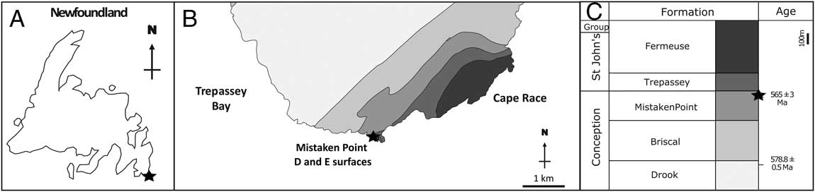
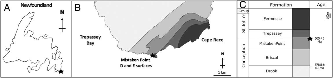
To assess the interspecific dynamics of Ediacaran Avalonian communities, we carried out a detailed BNI and SPPA of the D and E surfaces of the Mistaken Point Formation in SE Newfoundland (Fig. 1). These two surfaces host the most abundant and best preserved communities of Avalonian macrofossils on record (Liu et al. Reference Liu, Kenchington and Mitchell2015), dated to 565±3 Ma (Benus Reference Benus1988). The fossils are preserved as external molds in siltstone hemipelagites, cast from above by volcaniclastic deposits (Wood et al. Reference Wood, Dalrymple, Narbonne, Gehling and Clapham2003; Ichaso et al. Reference Ichaso, Dalrymple and Narbonne2007). This study uses the data set of Mitchell et al. (Reference Mitchell, Kenchington, Liu, Matthews and Butterfield2015), comprising 2977 fossil specimens from the E surface and 1402 specimens from the D surface (Supplementary Fig. S1). The mean accuracy of the GPS coordinates of the data was 0.460±0.06 cm horizontally and 0.8260±0.11 cm vertically. All fossils with a consistently recognizable form were assigned to 10 taxonomic groupings (cf. Clapham et al. Reference Clapham, Narbonne and Gehling2003): Bradgatia, Charniid, Charniodiscus, Fractofusus, Hiemalora, Ivesheadiomorphs, Lobate Discs, Pectinifrons, Plumeropriscum, and Thectardis. For completeness, all remaining specimens were placed in one of two “bin groups”: Holdfast Discs and Other Species (see Supplementary Fig. S2 and Section S1 for taxonomic definitions).
Locality map showing: A, the location of Mistaken Point Ecological Reserve in Newfoundland, Canada; and B, the locations of D and E surfaces within the reserve, with the formations shown in grayscale, as given in C. C, Stratigraphic column showing radiometric dates and the locations of D and E surfaces (star). (Modified from Liu 2016: Fig. 1E,F.)
Spatial Analyses Performed on the D and E Surfaces at Mistaken Point
Two types of spatial analyses were performed on the spatial data of the D and E surfaces: BNI followed by SPPA (see Supplementary Section S2 for extended methods). Performing BNI prior to SPPA analyses ensures that bivariate correlations are not incorrectly linked to an interspecific ecological process, by distinguishing a connected series of indirect correlations between several taxa from one direct correlation between two taxa. Such BNI screening is not required with univariate PCF analyses, or bivariate analyses between differing size classes, because there is no possibility of indirect correlations. In principle, careful bivariate SPPA should be able to distinguish direct from indirect correlations; however, when dealing with problematic fossils, such as those of the Ediacaran Avalon, BNI provides a key check on whether the signals found are indeed genuine direct correlations.
Bayesian Network Inference
The set of correlations or “edges” between taxon pairs (networks) for both D and E surfaces was identified using BNI (Heckerman et al. Reference Heckerman, Geiger and Chickering1995). To find the best-fit network for each surface, the mapped areas were first divided into quadrats and discretized into zero, low, and high densities. Then 100 samples were created by bootstrapping (subsampling) these quadrat data sets at the 95% level (Magurran Reference Magurran2013), and the Bayesian network was calculated using the software Banjo (Smith et al. Reference Smith, Yu, Smulders, Hartemink and Jarvis2006). The resulting set of edges formed a bimodal distribution, represented by either rare–low occurrences or high occurrences. High-occurrence edges (determined using ‘mclust’; Fraley et al. Reference Fraley, Raftery and Scrucca2012) are the constituent edges of the underlying network, while the low-occurrence edges are random “noise” and do not correspond to actual correlations (cf. Yu et al. Reference Yu, Smith, Wang, Hartemink and Jarvis2004); the results are depicted in the form of network diagrams. The interaction strength is defined as the relative weight or strength of each high-occurrence edge output by Banjo, where 1 represents a strong positive correlation, −1 is a very strong negative correlation, and 0 is a nonmonotonic correlation (i.e., positive and negative at different spatial scales). Where a correlation between taxa was asymmetric (i.e., the strength and/or nature of one taxon on the other was not identical), this correlation was indicated on the network diagram by an arrow. Mann-Whitney tests were used to compare the effects of taxon, edge removal, and directionality and to assess the relative importance of each to the network.
Spatial Point-Process Analyses
Unlike the BNI assessment of whole-community structure, PCF analyses can only consider an individual taxon (univariate) or pairs of taxa (bivariate) during one set of analyses. To describe an entire community structure, all individuals within the community need to be accounted for, hence the inclusion of obvious organ–taxa (Hiemalora) and bin groups (Holdfast Discs and Other Species) in the BNI analyses. At the same time, however, the taxonomic indeterminacy of such groups is likely to obscure any paleoecological signal based on their spatial distributions. As such, these groups have been omitted from follow-up PCF analyses and discussion. Putative taphomorph taxa, which may include carcasses and associated decay-induced microbial colonies (cf. Darroch et al. Reference Darroch, Laflamme and Clapham2013) such as Ivesheadiomorphs and Lobate Discs, are included in the PCF analyses because they are both morphologically and taphonomically distinct from all of the other taxonomic groups. Form-taxonomic groups that are likely to include a range of “natural” taxa (e.g., Holdfast Discs, Other Species, Hiemalora) do not have equivalent extant ecological models with which to interpret the correlations, so they are excluded from the bivariate PCF analyses.
Initial data exploration and heterogeneous Poisson modeling were performed in R using the package ‘spatstat’ (Baddeley et al. Reference Baddeley, Rubak and Turner2015; Supplementary Methods S2). Three types of SPPA were used to determine the most likely underlying process behind each interspecific interaction found using BNI: (1) PCFs, (2) model fitting to the PCFs, and (3) RLAs. Programita was used to find PCFs and to perform aggregation model fitting (Wiegand and Moloney Reference Wiegand and Moloney2004, Reference Wiegand and Moloney2013; Wiegand et al. Reference Wiegand, Kissling, Cipriotti and Aguiar2006, Reference Wiegand, Martínez and Huth2009). Monte Carlo simulations and Diggle’s goodness-of-fit test were used to compare the fit of different spatial model PCFs to the observed PCFs (the p-value p d , in which p d =1 indicates a complete model fit, and p d =0 indicates no fit [Diggle Reference Diggle2003; Illian et al. Reference Illian, Penttinen, Stoyan and Stoyan2008]) and to determine the occurrence of habitat associations, competition, and facilitation between taxon pairs. Note that the p d is not a probability, but more akin to the coefficient of determination (R 2) in a linear regression, wherein the value represents the percentage of the data described by the model. Finally, RLAs were used to detect density-dependent mortality processes (Jacquemyn et al. Reference Jacquemyn, Endels, Honnay and Wiegand2010; Raventós et al. Reference Raventós, Wiegand and De Luis2010) using Monte Carlo simulations and calculating the difference in the extent to which each taxon departs from random labeling; that is, whether the two populations exhibit density dependence. Because this measure is a difference between two PCF quotients, p d RLA=0 corresponds to a random RLA pattern between the two taxa, indicating no density dependence; by contrast, p d RLA=1 indicates no distribution overlap and spatial patterning that is fully density dependent. These spatial analyses and their relationships to ecological processes are outlined below; the underlying mathematics is described in detail by Wiegand and Moloney (Reference Wiegand and Moloney2004) and Wiegand et al. (Reference Wiegand, Kissling, Cipriotti and Aguiar2006).
Using Spatial Point-Process Analyses to Detect and Describe Interspecific Interactions
In the case of sessile communities, there are just four principal interspecific processes that influence interspecific distributions: (1) habitat associations (colocation of two taxa on the same habitat), (2) competition (one or both taxa limit a mutual resource), (3) facilitation (one taxon enhances the survival of another), and (4) differential mortality/density-dependent effects (Wiegand et al. Reference Wiegand, Gunatilleke and Gunatilleke2007a). Each of these processes is best described by a distinct spatial point-process model, so comparison of observed bivariate spatial distributions to these models can resolve the underlying process(es) (Diggle Reference Diggle2003; Wiegand and Moloney Reference Wiegand and Moloney2004). Although these models have been developed primarily in the context of terrestrial forest ecology, the underlying principles are equally applicable to other communities of sessile organisms, including fungal sporocarps (e.g., Liang et al. Reference Liang, Guo, Du and Ma2007) and nonmotile animals (e.g., Muko et al. Reference Muko, Shimatani and Nozawa2014).
Bivariate or pairwise PCFs describe how the densities between specimens belonging to two different taxa change with spatial scale, thus capturing interspecific patterns. A bivariate PCF=1 corresponds to two populations that exhibit CSR with respect to one another; that is, they have no pairwise spatial structure and their bivariate distribution can be modeled by a homogeneous Poisson process (Illian et al. Reference Illian, Penttinen, Stoyan and Stoyan2008). Accordingly, if a homogeneous Poisson model is the best fit to the data (i.e., exhibits CSR), then the constituent organisms do not exhibit any significant interactions. Insofar as most co-occurring taxa in most ecosystems are likely to exhibit some degree of interaction, sessile communities with no spatial structure are unusual, typically seen only during early establishment and/or when resources are unlimited (e.g., Greig-Smith Reference Greig-Smith1979; Lin et al. Reference Lin, Chang, Yang, Wang and Sun2011; Wiegand et al. Reference Wiegand, Huth, Getzin, Wang, Hao, Gunatilleke and Gunatilleke2012).
By contrast, a bivariate PCF≠1 indicates statistically significant aggregation (PCF>1) or segregation (PCF<1) between taxa. The magnitude of the PCF reflects the intensity of underlying biological and physical processes: two taxon populations with a PCF=4, for example, are four times more aggregated than if they exhibited CSR; thus, the relative magnitudes of the PCFs can be used to compare relative strengths of interactions and associations.
Habitat Associations
Habitat associations occur when two (or more) taxa have the same environmental preferences, such as the aggregation of alpine tree species at a common altitude (Wang et al. Reference Wang2011) or aggregations around a patchy distribution of soil nutrients (John et al. Reference John2007). Where interspecific interactions derive from such habitat associations, they can be modeled by shared-source models (also called shared-parent models) in which the two sets of taxa aggregate around the same set of mutually exclusive points; that is, the focus of the taxon clusters are points that are not biological taxa but some other “environmental” factor (Wiegand et al. Reference Wiegand, Gunatilleke and Gunatilleke2007a). Where habitat associations are shared between more than two taxa, they can be described by heterogeneous Poisson models, whereby specimen density is modeled by a random process in which density varies across the sample area depending on the given variable (e.g., altitude). Differing sensitivities to habitat heterogeneities can be encapsulated by using differing radii to form the heterogeneous Poisson model that describes the habitat (Supplementary Appendix S2). Use of smaller radii to form the heterogeneous background corresponds to a stronger (more sensitive) reaction to the habitat, while use of larger radii corresponds to a weaker (more diffuse) reaction. Heterogeneous habitats formed from different substrate variations are quantified by different parameters of the bivariate shared-source model, such as the mean patch/cluster radius, the total number of patches/clusters, and the mean number of specimens within each patch/cluster. When two bivariate models have different parameterizations, two distinct underlying substrate variations will have been identified, a reflection of ecological differences between the associated taxa.
Competition between Taxa
Among sessile organisms, competition over limited resources is typically expressed in the form of reduced specimen density, a process known as thinning. In forests, thinning of fast-growing but shade-intolerant pioneer species occurs as a consequence of progressive light competition (Getzin et al. Reference Getzin, Dean, He, Trofymow, Wiegand and Wiegand2006). In spatial terms, such interspecific competition is detected as segregation between taxa, wherein the segregation is demonstrably not due to an association with a habitat that is itself patchy (in which case the pattern would fit a bivariate shared-source or heterogeneous Poisson model; see Wiegand et al. Reference Wiegand, Gunatilleke and Gunatilleke2007a).
Interspecific competition is scale-dependent, with preemptive and interference competition acting on smaller spatial scales, and resource competition acting over larger spatial scales. In modern corals, for example, segregation often occurs when one taxon excludes another by preemptively occupying substrate space, yielding a system in which the size of individual coral heads corresponds to local levels of (preemptive) competition (McCook et al. Reference McCook, Jompa and Diaz-Pulido2001). In this case the pattern can be recognized spatially by small-scale thinning or segregation, which occurs at similar magnitudes to the occupying taxon. At larger scales, however, such direct interspecific competition may derive from the active release of inhibitory biochemicals (allelopathy), disabling the settlement and/or survival of their neighbors and yielding a quantitatively distinct spatial distribution (Willis Reference Willis2007). By assessing small-scale segregation in the context of body size, it is possible to distinguish these distinct types of competition. Large-scale segregation can be distinguished from mutual association over a habitat of segregated patches by assessing whether heterogeneous Poisson models (i.e., local habitat heterogeneities) can be used to describe the large-scale segregations (Wiegand et al. Reference Wiegand, Gunatilleke, Gunatilleke and Okuda2007b). Thus, comparison of the spatial scales of segregations and of segregated distributions using heterogeneous Poisson and shared-source models (to detect habitat associations) can be used to detect competition and infer the most likely underlying process.
Facilitation
Interspecific facilitation is a process whereby the presence of one taxon benefits the survival of another (e.g., Brooker et al. Reference Brooker2008). Facilitation can be physical, such as protection from harsh conditions or the creation of suitable habitat (Jones et al. Reference Jones, Lawton and Shachak1997), or intimately biotic, as encountered in mutualistic endosymbioses (e.g., Bruno et al. Reference Bruno, Stachowicz and Bertness2003). In spatial terms, facilitation is indicated when the best-fit bivariate is a linked-cluster or double-cluster model (also known as bivariate Neymann-Scott/Thomas cluster models). In linked-cluster models, the spatial pattern is described by a series of clusters with normally distributed densities (i.e., Thomas clusters) centered on the positions of the facilitating taxa (Dickie et al. Reference Dickie, Schnitzer, Reich and Hobbie2005; Dale and Fortin Reference Dale and Fortin2014). A linked Thomas double-cluster pattern is induced when the facilitated taxon (which forms Thomas clusters around the facilitating taxon) reproduces to form secondary Thomas clusters, resulting in Thomas double clusters, each centered on specimens of the facilitating taxon. Mutualisms are best modeled by a heterogeneous Poisson process with a density created from the joint density of the two taxa, which indicates mutual clustering with no external driving factor.
Density-dependent Mortality Processes
Mortality rates within a population can vary due to a variety of density-dependent processes, potentially influencing community spatial distributions and structure. For example, the high biodiversity of tropical forests appears to be maintained through Janzen-Connell effects, whereby taxon-specific consumers such as herbivores or pathogens generate (positive) density-dependent mortality of their prey taxa. Janzen-Connell effects prevent any single taxon from dominating the community, thus maintaining high community diversity (Velázquez et al. Reference Velázquez, Kazmierczak and Wiegand2016). Mortality processes can be investigated using RLAs (Goreaud and Pélissier Reference Goreaud and Pélissier2003; Raventós et al. Reference Raventós, Wiegand and De Luis2010), wherein the spatial positions of the organisms are held constant, but a specimen property such as size class or preservation detail is randomly shuffled among the observed spatial positions using Monte Carlo simulations. If the observed pattern falls outside this generated simulation envelope, then the specimen property (subgroup) is nonrandomly distributed within the community population and a density-dependent process is detected. RLAs have been used to interrogate the effects of fire and canopy gaps on forest ecosystems and postfire succession (De Luis et al. Reference De Luis, Raventós, Wiegand and González-Hidalgo2008; Getzin et al. Reference Getzin, Wiegand and He2008). They can also be employed to compare the spatial distributions of superficially distinct forms, such as juveniles or differentially degraded carcasses.
Application of Spatial Point-Process Analyses to Identify Taphomorphs
Identification of taphomorphs is crucial to ensure an accurate ecological understanding of Avalonian communities, ensuring that any impact of time-averaging can be identified and the relative importance of decay-based processes assessed. Unlike extant communities, in which living and dead specimens are easily distinguished, identifying preserved taphomorphs is impeded within Avalonian communities, because the distinction between true morphological characters and taphonomically degraded characters is not well defined (e.g., Antcliffe et al. Reference Antcliffe, Hancy and Brasier2015); and more generally Avalonian morphological characters are limited in number compared with Phanerozoic organisms (e.g., Dececchi et al. Reference Dececchi, Narbonne, Greentree and Laflamme2017). However, comparison of the bivariate spatial distributions of putative taphomorphs with those of non-taphomorph taxa can be used to establish both the likelihood of taphomorphic affinity and, for taphomorphs, their precursor taxa: whereby, the spatial distributions of taphomorph taxa are expected to mirror those of their precursor taxa, that is, to be nonunique. Note that these analyses assume that there is no patchy small-scale degradation (reflected by intraspecific segregation), a pattern that is not encountered on the D or E surfaces (Mitchell et al. Reference Mitchell, Kenchington, Liu, Matthews and Butterfield2015). In this context, taphomorphs are expected to exhibit a random distribution within their precursor taxon populations and to have similar bivariate correlations. Ecological interpretations of taphomorph distributions need to take their affinity into account, because when taphomorphs mirror the spatial distributions of their precursors, a competitive-type spatial distribution can be detected, for example, not because the taphomorphs are directly competing with another taxon, but because the precursor taxon to the taphomorph did compete with that taxon.
Ivesheadiomorphs and Lobate Discs (Supplementary Fig. S2J, F) are the two dominant putative taphomorphs found within Mistaken Point communities (Clapham et al. Reference Clapham, Narbonne and Gehling2003). Ivesheadiomorphs are characterized by a lack of consistent internal or external form, low preservation detail, and rarity of symmetrical features (Liu et al. Reference Liu, Mcilroy, Antcliffe and Brasier2011). Lobate Discs are also relatively irregular compared with other taxonomic groups such as the rangeomorphs, but they are characterized by a circular shape with high relief, and approximately radially symmetrical, irregular lobes. Both putative taphomorphs have a high morphological variability within identified specimens that, when coupled with differences in spatial distributions due to the differing impact of local habitat heterogeneities and/or differing times of community development, means that their affinities should be assessed on a surface-by-surface basis. In other words, identification of any taphomorph and its precursor taxa on one surface may not apply to another surface (Kenchington and Wilby Reference Kenchington and Wilby2014).
Results and Discussion
Our analyses focused on the D- and E-surface communities of Mistaken Point, SE Newfoundland. The E surface is the most diverse and abundant assemblage of Avalonian fossils on record, preserving 14 distinct species (with 8 abundant taxa) and 2977 identifiable specimens within its 63.5 m2 area (Clapham et al. Reference Clapham, Narbonne and Gehling2003; Mitchell et al. Reference Mitchell, Kenchington, Liu, Matthews and Butterfield2015). The Mistaken Point D surface is also taxonomically diverse, preserving 8 identifiable species (with 3 abundant taxa) within its 62.0 m2 area and 1402 individual fossils. Combined BNI and advanced SPPA provided an unprecedented level of ecological insight into the two principle surfaces, and revealed ecological distinctions between them beyond differences in community composition (cf. Clapham et al. Reference Clapham, Narbonne and Gehling2003).
BNI
E Surface
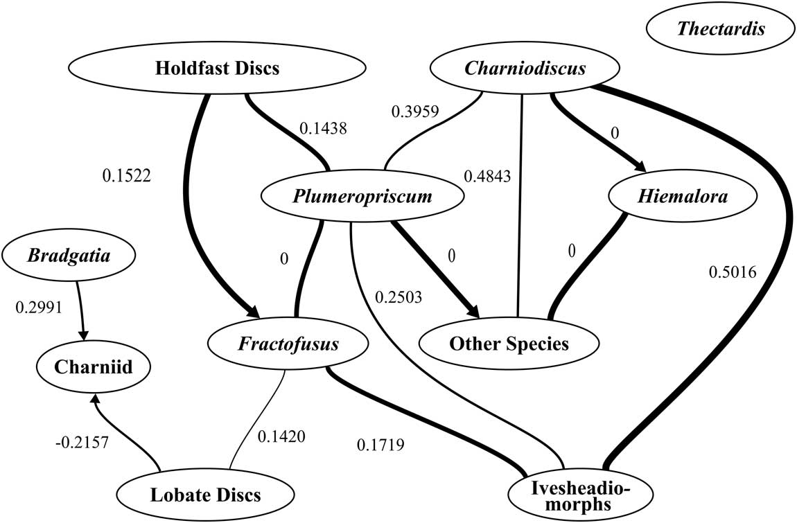
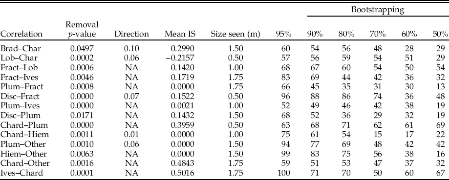
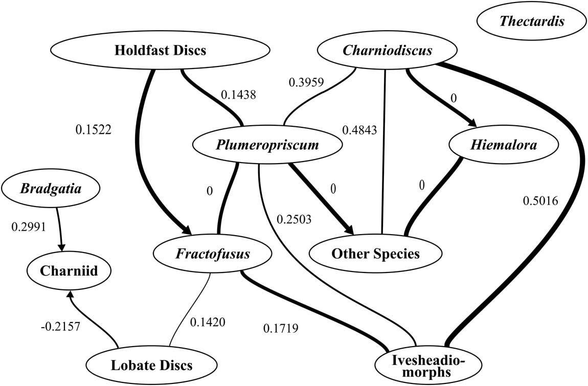
On the E surface, BNI analysis revealed a complex network of interspecific interaction and associations between the 11 taxonomic groups identified in this study (Fig. 2). Out of a possible 66 correlations, we identified 14 interspecific correlations involving all but one of the constituent taxa, Thectardis. On average, each taxon interacted with at least two other taxa (2.41 mean per taxon correlation); though interaction strengths were skewed toward low values (0.17 mean interaction strength). There were four nonmonotonic correlations (different positive and negative correlations at different spatial scales), one negative correlation, and nine positive correlations (Table 1). Fractofusus and Plumeropriscum were the most connected taxa, with four correlations each: Fractofusus correlated with Plumeropriscum, Ivesheadiomorphs, Lobate Discs, and Holdfast Discs; Plumeropriscum correlated with Fractofusus, Charniodiscus, Holdfast Discs, and Other Species. Bradgatia was the least connected taxon within the network, only correlating with the Charniid group. Excluding Hiemalora and the two bin groups resulted in eight interspecific correlations among the eight remaining taxa—with a mean per taxon correlation of 2.28 and a mean interaction strength of 0.19.
Bayesian network for the E surface. Correlations are indicated by lines connecting the taxon pairs. The occurrence rate is indicated by the width of the edge (the line depicting correlation between two taxa); the wider the line, the higher the occurrence rate. Arrows indicate nonmutual dependence between two taxa; for example taxon 1 is aggregated with respect to taxon 2, but taxon 2 is not aggregated with respect to taxon 1. Numbers by the lines are the mean interaction strengths of the correlations, with positive interaction strengths indicating aggregation, negative interaction strengths indicating segregation, and zero indicating different aggregation and segregation behaviors at different densities.
Edge properties for the Bayesian network given in Fig. 4. The column labels are defined as follows: Removal p-value: The p-value for whether the network score (the fit of the network onto the data) is significantly different if that correlation is removed. Direction: The p-value for whether the network score is significantly different if the direction of that correlation is reversed. Mean IS: The mean interaction strength of all the networks bootstrapped at 95%. Size seen (m): The smallest quadrat size at which the correlation is detected. Bootstrapping 95%: The occurrence rate for the 95% bootstrapped networks that indicates consistency of correlation over different quadrats of the bedding plane. Bootstrapping 90–50%: The occurrence rates for the bootstrapped data when subsampled at the 50%, 60%, 70%, 80%, and 90% levels. See SI Methods for bootstrapping details. NA indicates mutual correlations. The following taxon notation is used: Brad, Bradgatia; Char, Charniid: Chard, Charniodiscus: Plum, Plumeropriscum: Fract, Fractofusus: Hiem, Hiemalora: Ives, Ivesheadiomorph: Lob, Lobate Discs.

The only taxon on the E surface to show no interspecific interactions or associations was Thectardis (based on 10,000,000 networks from 100 95% bootstrap samples; Fig. 2), which could be selectively excluded from the analyses without changing the network (p=0.54; Fig. 2; Table 1). This result is not due to low abundance of Thectardis (<1% of E-surface specimens): the BNI data are input using discrete values, so the absolute abundance does not influence the network output. Moreover, taxa with similar abundances (Hiemalora and Bradgatia) interact with other taxa even at the lower sampling of 80% BNI (Table 1). As such, the absence of Thectardis from the recovered network is most likely to be a real ecological signal, demonstrating its ecological isolation from other E-surface taxa. In addition to its conspicuously unconnected spatial distribution, Thectardis also stands out morphologically, distinguished by a simple triangular outline (Supplementary Fig. S3D) and absence of the fractal or frondose differentiation seen in most co-occurring forms. Sperling et al. (Reference Sperling, Peterson and Laflamme2011) have speculated on its possible sponge affiliations, but with little corroborating evidence (Antcliffe et al. Reference Antcliffe, Callow and Brasier2014). The ecological disparity of Thectardis is consistent with Thectardis having a different feeding mode than the other E-surface taxa, for example, the active filter feeding that sponges employ, versus the passive osmotrophic feeding of the Rangeomorphs. As such, our spatial analyses are consistent, but not definitive, in the support of a sponge affinity for Thectardis.
D Surface
Despite the comparably abundant and diverse assemblage of the D surface, BNI analysis found no bivariate correlations between the three abundant taxa (Fractofusus, Bradgatia, and Pectinifrons), while the remaining five (Plumeropriscum, Charniodiscus, Ivesheadiomorphs, Charniid, and Lobate Discs) occur in too low an abundance (<30 specimens/taxon) to yield statistically significant results. As such, there are no reportable correlations or interaction strengths for the D surface and no potential for follow-up SPPA analysis. The only nonrandom PCF distribution on the D surface is the univariate distribution of Fractofusus (Mitchell et al. Reference Mitchell, Kenchington, Liu, Matthews and Butterfield2015).
The marked disparity in bivariate correlations between the D and E surfaces points to fundamental differences in their respective community structures, though only if the respective data sets are taphonomically comparable. It is notable, for example, that the overall density of fossils on the D surface is ~50% that of the E surface (Clapham et al. Reference Clapham, Narbonne and Gehling2003; Mitchell et al. Reference Mitchell, Kenchington, Liu, Matthews and Butterfield2015), which could potentially derive from differential modern erosion (cf. Matthews et al. Reference Matthews, Liu and McIlroy2017). Our subsampling of the E-surface community to a similar density as the D surface (50%), however, found that 3 of its 14 correlations were still readily detectable (Table 1), demonstrating significant signal retention. Moreover, the three abundant D-surface taxa have a total density comparable to that of their counterparts on the E surface (2.27–22.40 specimens/m2 vs. 0.62–20.70 specimens/m2, respectively), while the E-surface pairwise densities of both Bradgatia+Charniid and Charniid+Lobate Discs are greater than the pairwise densities of D-surface taxon pairs. At least in the case of these taxa and pairwise densities, it is clear that the absence of correlations on the D-surface is not an artifact of differential preservation or sampling. The differences are ecological.
Another possible interpretation of the disparity in BNI results between E and D is that the lower specimen density of D represents an early stage of community succession, yet to put pressure on local resources (Townsend et al. Reference Townsend, Begon and Harper2003); that is, the organisms have not yet reached sufficient densities to be impacted by each other or their habitat. The presence of at least two generations of Fractofusus (Mitchell et al. Reference Mitchell, Kenchington, Liu, Matthews and Butterfield2015), however, demonstrates substantial community development. As such, the absence of ecological interactions, or even interspecific correlation, on the D surface is more likely to reflect a more homogeneous background environment than that of E surface; in the absence of habitat/resource patchiness, there was minimal competition. Habitat heterogeneity is generally correlated to taxonomic diversity (e.g., Agarwal Reference Agarwal2008), so the reduced diversity of the D surface might be a simple consequence of the homogeneous environment.
Spatial Point-Process Analyses of the E Surface
Using bivariate PCF analyses, we found seven of the eight E-surface correlations to be habitat associations and one to be the result of preemptive competition (Fig. 3; Supplementary Table S1). Within the habitat associations, two were devoid of any discernible interaction beyond colocation, three exhibited nonunique or mirrored behaviors (Supplementary Table S2), and two showed clear evidence of subsequent behavior. There was no evidence of facilitation between any of the taxa on the E surface.
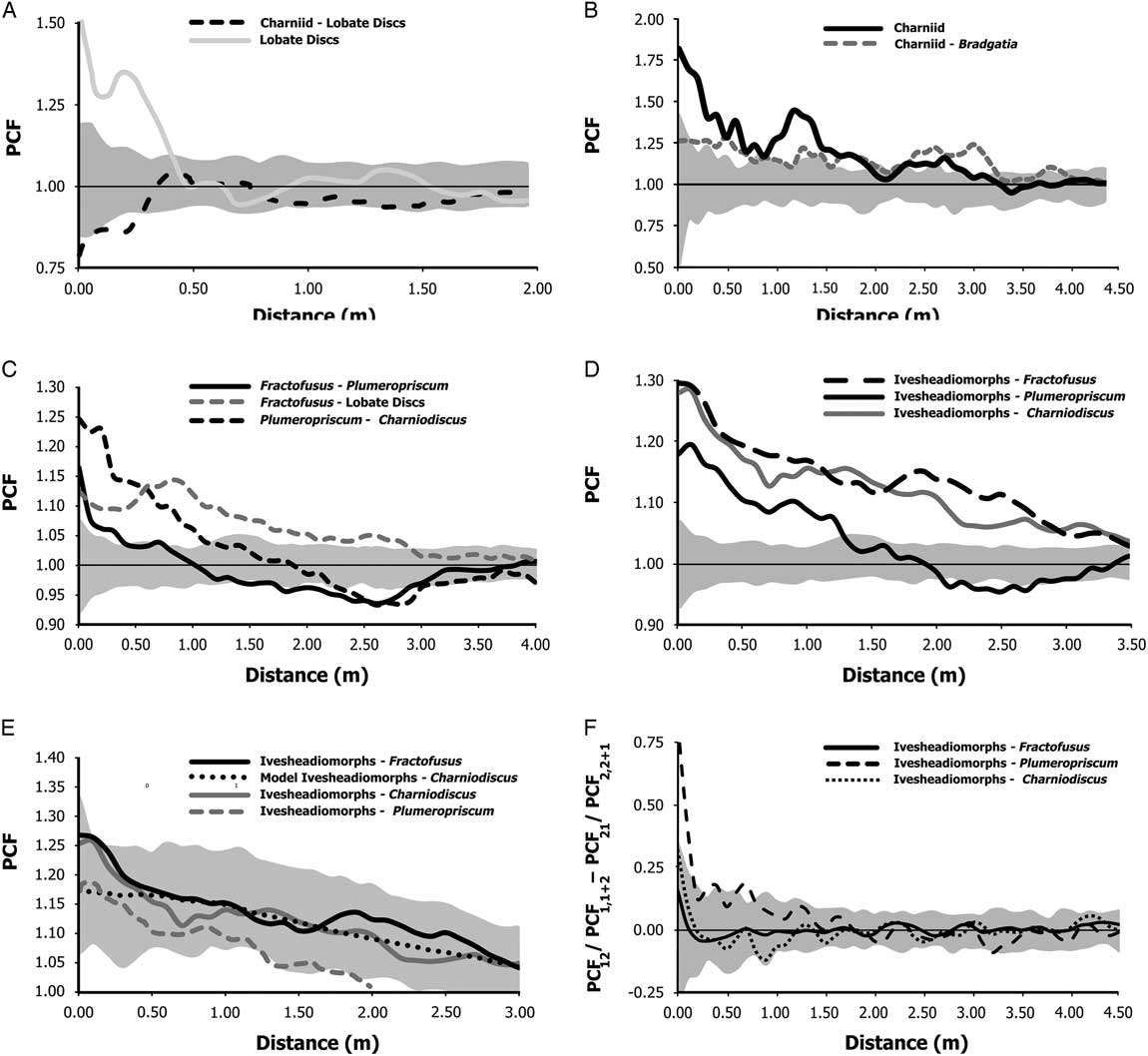
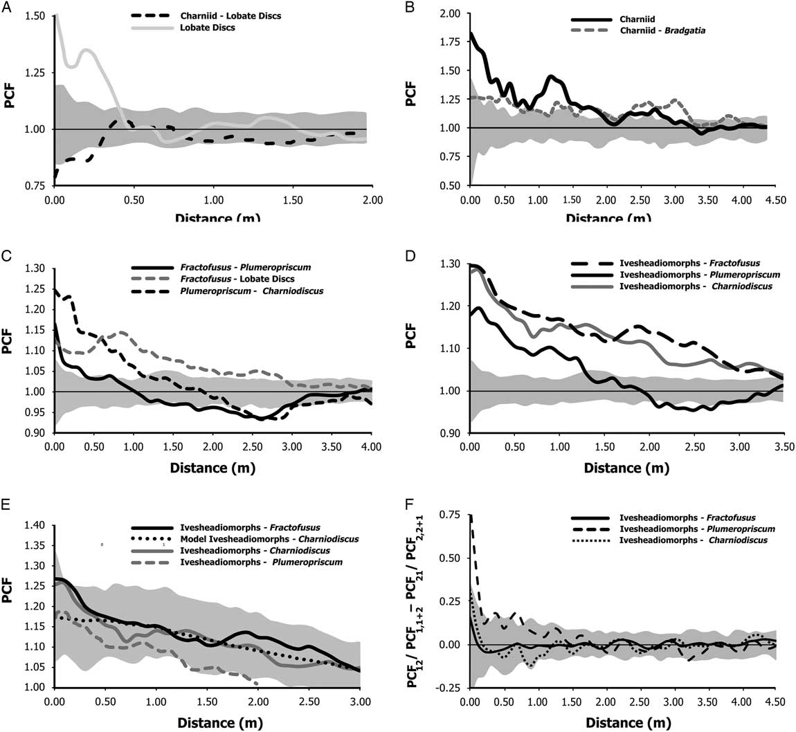
Pair-correlation functions (PCFs) for the E surface. The x-axis is the interpoint distance between organisms in meters. On the y-axis, PCF=1 indicates complete spatial randomness (CSR), <1 indicates segregation, and >1 indicates aggregation. A, Charniid–Lobate Discs bivariate distribution and Lobate Discs univariate distribution. Gray shaded area is the boundaries of 99 Monte Carlo simulations of the CSR bivariate distribution. B, Charniid–Bradgatia bivariate distribution and Charniid univariate distribution. Gray shaded area is the boundaries of 99 Monte Carlo simulations of the CSR bivariate distribution. C, PCFs of non-Ivesheadiomorph bivariate distributions of Fractofusus and Plumeropriscum. Gray shaded area is the boundaries of 99 Monte Carlo simulations of the CSR bivariate distribution of Fractofusus–Plumeropriscum. D, Bivariate PCFs of Ivesheadiomorphs interactions. Gray shaded area is the boundaries of 99 Monte Carlo simulations of the CSR bivariate distribution of Ivesheadiormorphs–Plumeropriscum. E, Bivariate PCFs of Ivesheadiomorphs interactions showing the best-fit shared-source model of Ivesheadiomorphs–Charniodiscus. Gray shaded area shows the boundaries of 99 Monte Carlo simulations for the best-fit shared-source model of Ivesheadiomorphs–Charniodiscus. F, Random-labeling analysis results for the Ivesheadiomorphs distributions. On the y-axis, PCF=0 indicates CSR. Gray shaded area is the boundaries of 99 Monte Carlo simulations of the CSR randomly labeled distributions.
Preemptive Competition
Lobate Discs segregated from Charniid on spatial scales smaller than 0.5 m at a PCF of 0.75, reducing Charniid density by 21% (PCFmin=0.79; Fig. 3A; Supplementary Table S1). This small-scale segregation of Lobate Discs and Charniid is of the same spatial scale as the mean radius of Lobate Discs (Clapham et al. Reference Clapham, Narbonne and Gehling2003), suggesting that the segregation is due to preemptive competition of Charniid not settling directly on the Lobate Discs. An alternative taphonomic explanation, in which Charniid is preferentially degraded in association with Lobate Discs, is unlikely given the absence of such effects with co-occurring rangeomorphs such as Bradgatia or Plumeropriscum. Allelopathy also causes small-scale segregation, but in this case the Lobate Discs–Charniid correlation exhibits the same spatial scale as the univariate Lobate Discs (albeit nonsignificant) aggregation (Fig. 3A), suggesting that the underlying phenomenon did not extend more broadly, the expected pattern with chemical exclusion. That said, other chemical processes could result in such segregation if the inhibitory compound(s) remained localized within the Lobate Discs–occupied substrate, one possibility being the hydrogen sulfide scenario proposed by Dufour and McIlroy (Reference Dufour and McIlroy2017).
Interpreting the mechanisms behind the Lobate Discs–Charniid segregation is substantially hampered by the problematic nature of Lobate Discs, which lack a formal taxonomical definition or basic biological resolution; current interpretations range from a distinct macroscopic taxon to microbial colonies, taphomorphs, or even sedimentary intrusions (e.g., Laflamme et al. Reference Laflamme, Schiffbauer and Narbonne2011; Liu et al. Reference Liu, Mcilroy, Antcliffe and Brasier2011). Nonetheless, the statistical evidence for segregation is unambiguous and demonstrates that the Lobate Discs were largely in place before Charniid establishment.
The absence of allelopathy within the E-surface community contrasts with extant marine sessile communities, in which such chemical-based exclusion and other direct interference competition such as overgrowth competition is pervasive (e.g., Jackson and Buss Reference Jackson and Buss1975; Engel and Pawlik Reference Engel and Pawlik2000). Modern communities of sessile deep-sea organisms also tend to be densely packed, with corals and sponges commonly occupying 90% or more of available substrate (e.g., Calle Reference Calle2010). By contrast, even the relatively dense E-surface community has conspicuously lower substrate occupation rates (<13%; Clapham et al. Reference Clapham, Narbonne and Gehling2003), reflecting correspondingly lower levels of substrate competition. Even so, the univariate Charniid PCF shows strong environmentally mediated spatial distributions (Supplementary Fig. S3; Mitchell et al. Reference Mitchell, Kenchington, Liu, Matthews and Butterfield2015), suggesting that they may be more susceptible to the local substrate differences induced by the presence of Lobate Discs.
Unique Habitat Associations
PCF analyses found that seven bivariate correlations were most likely due to habitat associations, wherein both the constituent taxa experienced enhanced survival related to some (otherwise unseen) aspect of the background environment (Fig. 4A). Two of these seven unique habitat associations resulted in large-scale aggregations (Bradgatia–Charniid and Fractofusus–Lobate Discs; Fig. 3B,C), but without reducing the longer-term survival of either taxon (as would have been detected by segregation in the bivariate PCFs). The Bradgatia–Charniid correlation is a relatively consistent aggregation that corresponds to a mutual density increase of Bradgatia and Charniid by 15% above CSR up to a 3.4-m radius (PCFmax=1.15; Fig. 3B). The greatest aggregation of Bradgatia and Charniid occurs under an 0.8-m radius (PCFmax=1.3) and is best modeled by a shared-source model (pd=0.66; Fig. 3B). This habitat heterogeneity also impacts Charniid, which is inferred by the similar spatial scales of the aggregated part of the univariate Charniid and bivariate Charniid–Bradgatia spatial distributions, but only very weakly affects Bradgatia, as reflected in its random univariate PCF (Fig 3A–C). The Charniid–Bradgatia spatial pattern is much weaker than that of the univariate Charniid aggregation, suggesting that this habitat heterogeneity strongly promotes Charniid establishment and only weakly promotes Bradgatia establishment. A similar pattern is observed in corals, where settlement is dependent on the type of previously established algae (cf. Carlon and Olson Reference Carlon and Olson1993). Univariate Charniid and the bivariate Charniid–Bradgatia are the only PCFs that correlate at this spatial scale (Fig. 3A–C), suggesting that this habitat heterogeneity did not affect other taxa on a meter scale.
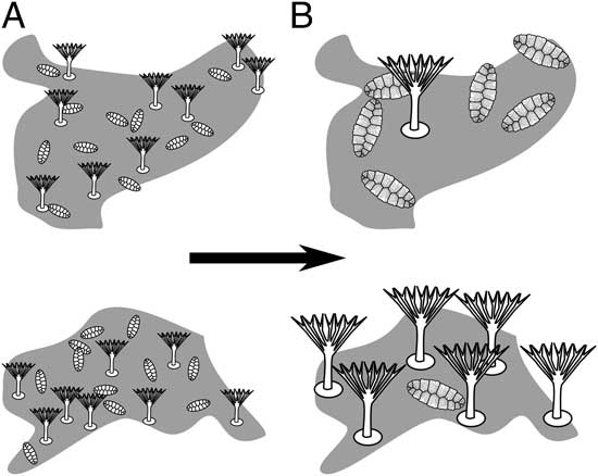
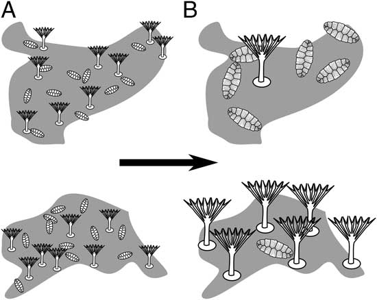
A, Reconstruction of the habitat association between Fractofusus–Plumeropriscum (SI Fig. 2I and 2B, respectively) resulting in mutual aggregation on top of the inferred heterogeneous habitat (gray shown in column A). In the case of Plumeropriscum–Fractofusus (and Plumeropriscum–Charniodiscus, not figured), these habitat associations result in competition for resources between mature specimens over time (depicted by the arrow), leading to thinning (segregation) of these larger individuals shown in column B. Note that only single generations are depicted to ensure the clarity of the process. More realistically, there would be multiple generations and different size classes (since these taxa reproduce continuously [Darroch et. al. Reference Darroch, Laflamme and Clapham2013]).
The E-surface Fractofusus–Lobate Discs correlation is consistent but weak (PCFmax= 1.15) up to a 2-m radius between these two taxa; it is best modeled by a shared-source model (p d =0.70; Fig. 3C). The association between Fractofusus and Lobate Discs does not exhibit the same spatial scaling as other univariate or bivariate spatial distributions (Fig. 3A–C) and could not be modeled by another best-fit bivariate model (Supplementary Table S2): as with Bradgatia and Charniid, it is a unique association. Notably, this pattern is a rare instance in which spatial pattern is evident in the field, with Fractofusus commonly observed to overlie Lobate Discs (cf. Dufour and McIlroy Reference Dufour and McIlroy2017).
Habitat Associations Leading to Competition
Both Plumeropriscum–Fractofusus and Plumeropriscum–Charniodiscus exhibit small-scale aggregation coupled with large-scale segregation (Fig. 3C). In the case of Fractofusus and Plumeropriscum, both taxa exhibit increased densities over a shared paleoenvironmental heterogeneity (as revealed by being best modeled by a shared-source pd=0.79; Fig. 3C; Supplementary Table S1), coupled with segregation (PCFmin=0.92 between 1.5 m and 3.5 m, reducing the established specimen density by 8.4%; Fig. 3C). Notably, this segregation could not be modeled by a heterogeneous Poisson model (Supplementary Tables S1 and S4). Such patterns most likely derive from interspecific resource competition, as growth leads to progressive thinning and spatial segregation of the most mature specimens (cf. Mason et al. Reference Mason2003; Fig. 4A,B). This same style of habitat association and resource competition is seen between Plumeropriscum and Charniodiscus and is similarly best modeled by a shared source (pd=0.97; Fig. 3C; Supplementary Table S1). The habitat associations between Plumeropriscum–Fractofusus and Plumeropriscum–Charniodiscus were significantly different, pointing to two distinct underlying aggregation sources (pd =0.04 and pd =0.01; Supplementary Tables S1 and S2), for example, variations in microbial mat coverage or depth.
Out of a possible 13 taxon pairs on the E surface, it is notable that interspecific resource competition is limited to just these two instances. The limited instances of interspecific competition stand in stark contrast to extant marine benthic communities and other sessile communities (such as terrestrial forests), where competition is ubiquitous (Bertness and Leonard Reference Bertness and Leonard1997; Wiegand et al. Reference Wiegand, Gunatilleke, Gunatilleke and Okuda2007b). These spatial differences also undermine the suggestion that Avalonian communities were similar in structure to extant benthic communities (Clapham et al. Reference Clapham, Narbonne and Gehling2003). At the same time, however, it is these three competing taxa—Fractofusus, Plumeropriscum, and Charniodiscus—that form the majority (58.6%) of the specimens on the E surface. In other words, although the majority of taxa do not exhibit interspecific resource competition, the majority of individuals appear to be competing for limited resources.
Importance of Using BNI Combined with Spatial Point-Process Analyses
SPPA applied to all possible pairwise combinations on the E surface revealed six nonrandom correlations not found by BNI. These derive from the combined effects of two unrelated correlations rather than direct interaction. Lobate Discs, for example, have a nonrandom PCF with respect to Plumeropriscum, but because this correlation was not found by BNI, the signal should be interpreted as a consequence of each taxon being separately correlated with Fractofusus. The presence of indirect, nonrandom PCFs that have a clear connection via an intermediate taxon highlights the importance of using BNI in combination with SPPA to minimize type I errors (false positives) when drawing paleoecological inferences.
Using Spatial Analyses to Identify Putative Taphomorphs
The D- and E-surface communities contain abundant populations of Ivesheadiomorphs and Lobate Discs, both of which have been widely viewed as the degraded taphomorphs of more “biological” taxa (Liu et al. Reference Liu, Mcilroy, Antcliffe and Brasier2011). Such interpretation clearly bears critically on any spatial analysis of Avalonian ecology, particularly on the E surface, where these two problematic forms represent 13.2% of all individuals and 46.7% of the total fossil area, a proxy for biomass (Clapham et al. Reference Clapham, Narbonne and Gehling2003). Our PCF and RLA analyses strongly support the identification of Ivesheadiomorphs as taphomorphs and identify the likely precursor taxa, but find that spatial distributions of Lobate Discs are inconsistent with a taphomorph affinity.
Ivesheadiomorphs’ Affinity and Precursor Taxa
PCF analyses found that Fractofusus–Ivesheadiomorphs was best modeled by a shared-source model (p d =0.65; Fig. 3D,E; Supplementary Table S1) as was Charniodiscus–Ivesheadiomorphs (p d =0.82). Neither the Fractofusus–Ivesheadiomorphs nor the Charniodiscus–Ivesheadiomorphs best-fit models were unique, and further analyses strongly suggest that Charniodiscus and Fractofusus are the precursor taxa of Ivesheadiomorphs on the E surface (cf. Liu et al. Reference Liu, Mcilroy, Antcliffe and Brasier2011) as follows: First, the Fractofusus–Ivesheadiomorphs and Charniodiscus–Ivesheadiomorphs correlations closely follow the univariate Fractofusus and Charniodiscus clustering (they exhibit the same small-scale high aggregation under 0.4 m (Fig. 3E). Second, the best-fit models for both correlations are heterogeneous Poisson models based on Fractofusus (for the Ivesheadiomorphs–Fractofusus correlation, p d =0.55) or Charniodiscus (for the Ivesheadiomorphs–Charniodiscus correlation, p d =0.75) densities. Likewise, the Fractofusus–Ivesheadiomorphs distribution could be modeled by the Plumeropriscum–Fractofusus correlation (p d =0.56) and vice versa (p d =0.71). And finally, the RLAs show that Ivesheadiomorphs are randomly distributed within both the Fractofusus and Charniodiscus populations (p d RLA <0.05 for both; Fig. 3F; Supplementary Table S3).
BNI of the E surface revealed a correlation between Ivesheadiomorphs and Plumeropriscum, which is best modeled by a shared-source model (p d =0.69; Fig. 3D,E; Supplementary Table S1), with a large-scale segregation of 95% CSR occurring between 2.0 and 3.5 m. However, corresponding SPPA rules out any precursor–taphomorph correspondence: the PCF of the Ivesheadiomorphs–Plumeropriscum distribution differs significantly from the univariate Plumeropriscum; the bivariate correlation of the two “taxa” cannot be modeled as a heterogeneous Poisson model using Plumeropriscum, and RLA also shows significantly different density-dependent behavior of Plumeropriscum relative to Ivesheadiomorphs, and there is further overlap with other bivariate models (Supplementary Tables S2 and S4): the Ivesheadiomorphs–Plumeropriscum correlation can be modeled by the same best-fit model as Fractofusus–Plumeropriscum (p d =0.58 for non-CSR PCF) and by Charniodiscus–Plumeropriscum (p d =0.55 for non-CSR PCF), pointing to closely comparable bivariate habits between Ivesheadiomorphs and both Fractofusus and Charniodiscus (that the combined 58% and 55% of these two spatial distributions exceed 100% is explained by a modest 25% overlap in the two models).
These three Ivesheadiomorphs correlations (Ivesheadiomorphs–Fractofusus, Ivesheadiomorphs–Charniodiscus, and Ivesheadiomorphs–Plumeropriscum) are notable in being the only observed correlations on the D and E surfaces that were nonunique. In other words, the spatial distributions of these pairwise correlations are statistically indistinguishable from the bivariate distributions of other pairs—in marked contrast to all other non-Ivesheadiomorphs correlations (Supplementary Table S2). The similarity of these Ivesheadiomorphs correlations with other E-surface correlations makes a microbial affinity (cf. Laflamme et al. Reference Laflamme, Schiffbauer and Narbonne2011) unlikely. Further, the inclusion of non-frondose Fractofusus within the Ivesheadiomorphs correlations is inconsistent with the interpretation of Ivesheadiomorphs as sediment intrusions beneath fronds (cf. Wilby et al. Reference Wilby, Carney and Howe2011), since there was no space between recumbent Fractofusus and the substrate that could be infilled by sediment.
Putative Non-Ivesheadiomorphs Taphomorphs
Apart from Ivesheadiomorphs, it has been argued that Lobate Discs (Liu et al. Reference Liu, Mcilroy, Antcliffe and Brasier2011), Thectardis, and Charniodiscus (Antcliffe et al. Reference Antcliffe, Hancy and Brasier2015) may also represent preservational variants of other (mostly unspecified) entities (as opposed to organ taxa, such as Hiemalora). Possible precursor taxa for Lobate Discs on the E surface are (the holdfasts of) Charniid, Charniodiscus, Bradgatia, and Plumeropriscum. None of these exhibit statistically similar bivariate spatial correlations, however, substantially undermining any taxonomic connection (Fig. 3D,E). Indeed, there are no frondose taxa on the E surface that could have been plausible precursors of Lobate Discs. By the same token, neither Charniodiscus nor Thectardis have univariate and bivariate spatial patterns that are statistically comparable to any co-occurring taxa, so they are unlikely to be taphomorphic variants (contra Antcliffe et al. Reference Antcliffe, Hancy and Brasier2015) (Mitchell et al. Reference Mitchell, Kenchington, Liu, Matthews and Butterfield2015; Fig. 2; Supplementary Fig. S3; Supplementary Table S2).
Multiple Successions
On a more general level, it is possible that the fossils preserved on any particular bedding surface belong to a succession of discrete communities; that is, not all were alive at the same time (cf. McIlroy and Garton Reference McIlroy and Garton2010; Liu et al. Reference Liu, McIlroy, Matthews and Brasier2012; Antcliffe et al. Reference Antcliffe, Hancy and Brasier2015). The BNI and SPPA results, however, are inconsistent with multiple colonization of the E surface, as are the univariate population analyses of Darroch et al. (Reference Darroch, Laflamme and Clapham2013) and the SPPA of Mitchell et al. (Reference Mitchell, Kenchington, Liu, Matthews and Butterfield2015). Significantly, size-distribution analyses of the E surface demonstrate single (not multiple) populations of abundant taxa (with the exception of Thectardis; Darroch et al. Reference Darroch, Laflamme and Clapham2013), and univariate spatial analyses find that there is no evidence of strong univariate environmental (habitat) influences in any E-surface taxa except Charniid (which eliminates bivariate correlations due to repeated successions being subject to the same environmental influence; Mitchell et al. Reference Mitchell, Kenchington, Liu, Matthews and Butterfield2015). As such, seven of the eight E-surface taxa can be recognized as contemporaneous. This reasoning cannot be applied to Thectardis, since it is not spatially correlated with any other taxon; however, its shared current alignment with frondose taxa on the same bedding surface suggests that it too was part of this community (Clapham et al. Reference Clapham, Narbonne, Gehling, Greentree and Anderson2004).
Taphomorph Ecology
Within Ediacaran communities, the habitat heterogeneity produced by decaying organisms has been proposed as the determining factor in community structure (Antcliffe et al. Reference Antcliffe, Hancy and Brasier2015; Budd and Jensen Reference Budd and Jensen2017; Liu et al. Reference Liu, Kenchington and Mitchell2015; Dulfour and McIlroy Reference Dufour and McIlroy2017). In this “Ediacaran-fall” model, localized concentrations of resources represented by macro-carcasses are likened to more recent whale-fall or wood-fall ecosystems (c.f. Smith et al. Reference Smith, Glover, Treude, Higgs and Amon2015), whereby decaying organisms form the focus of for colonizers to settle upon and form communities. When organisms feed directly on this carbon (or indirectly on the sulfides) produced by specimen decay, then the population densities of scavenger/saprophytic species tend to increase around the local resource, resulting in a spatial pattern best modeled as a linked cluster (or double-cluster) model or a heterogeneous Poisson model based on carcass densities (Wiegand and Moloney Reference Wiegand and Moloney2013). Notably, no such spatial patterns are observed with Ivesheadiomorphs on the Mistaken Point surfaces. Instead there is a mutual clustering around two different shared sources for Ivesheadiomorphs, one with Fractofusus and the other with Charniodiscus (Fig. 3D; Supplementary Table S1); that is, there is no increased survival for taxa that settle near Ivesheadiomorphs. The correlations between Ivesheadiomorphs–Fractofusus and Ivesheadiomorphs–Charniodiscus are most likely a reflection of the single-taxon clustering that occurs for both these taxa, with dead specimens (i.e., Ivesheadiomorphs) randomly distributed among the living. Thus, our spatial analyses refute the hypothesis that any single taxon (such as Fractofusus, Charniodiscus, or Plumeropriscum) was a scavenger. Alternatively, a habitat heterogeneity formed from unpreserved decayed carcasses could be detected as a habitat association between taxa. However, if several taxon pairs were impacted by the same single-decay heterogeneity, then they would be expected to share the same shared-source model, which is inconsistent with the four distinct habitat associations present on the E surface and the absence of any such associations or interactions on the D surface. Taken together, SPPA analysis rules out saprophytic habits as a controlling factor in structuring these Avalonian communities.
Conclusions
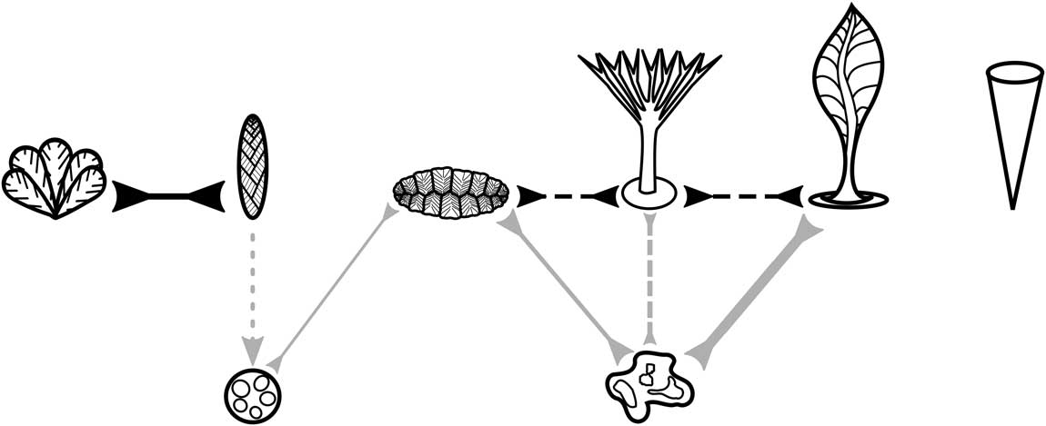
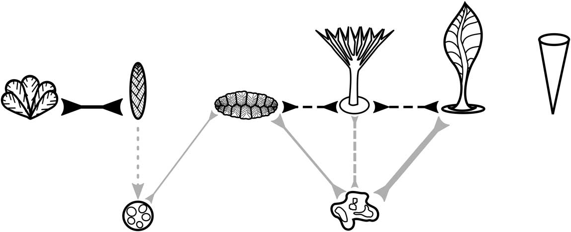
Our spatial analyses of the E surface at Mistaken Point reveal a fundamentally more complex community structure than has been previously recognized (Fig. 2), showing clear ecological differentiation between taxa, with all six abundant non-taphomorph taxa developing different responses to a variety of habitat spatial variations (Fig. 5; Supplementary Table S2). The presence of multiple ecological responses demonstrates that individual taxa have distinct approaches for adapting to local habitat, leading to divergent selection, reproductive isolation, and ultimately biodiversification (Kawecki and Ebert Reference Kawecki and Ebert2004; Mitchell-Olds and Schmitt Reference Mitchell-Olds and Schmitt2006; Hereford Reference Hereford2009; Sobel et al. Reference Sobel, Chen, Watt and Schemske2010; Futuyma and Agrawal Reference Futuyma and Agrawal2009). The fundamentally different degree of organismal interaction in these Avalonian communities demonstrates their fundamentally non-uniformitarian nature, highlighted by the complete lack of D-surface community interspecific interactions, and could well account for the conspicuously slow nature of their evolutionary turnover (cf. Grazhdankin Reference Grazhdankin2004). At the same time, the low levels of competitive interactions (e.g., in comparison to modern forests or deep-sea reefs) established in these earliest communities of macroscopic organisms sets the stage for progressive escalation; first through elevated competition for resources, then leading to macroscopic movement and, ultimately, carnivory.
Summary diagram of the E-surface bivariate interactions and associations. Top row from left: Bradgatia, Charniid, Fractofusus, Plumeropriscum, Charniodiscus, and Thectardis. Bottom row from left: Lobate Discs and Ivesheadiomorphs. Gray lines denote taxa with unknown or disputed affinities, while black indicates interactions and associations between living-at-time-of-burial organisms. Two inward arrows indicate mutual habitat associations; solid lines indicate only these habitat associations, while long dashes indicate that these associations result in resource competition. Arrow with dotted line depicts preemptive competition.
This study has demonstrated how new approaches to spatial analysis can resolve key aspects of Avalonian paleoecology. By combining BNI with PCFs, it is possible to describe the spatial variation of specimen densities between taxon pairs, establishing when taxa are responding to one another and/or their habitat. Model fitting takes these analyses beyond descriptive statistics, enabling verifiable predictions to be made and ecological hypotheses to be tested. RLA enables the comparison of density-dependent behavior within a given spatial pattern, thus assisting in the identification of taphomorphs. These techniques present a framework for further investigations, which can incorporate morphological details such as body size to investigate broader ecological themes such as the implications of tiering and/or ecological successions on Ediacaran community structure.
Acknowledgments
Environment and Conservation, Government of Newfoundland and Labrador provided permits to conduct research within the Mistaken Point Ecological Reserve in 2010. Access to the aforementioned fossil localities is by scientific research permit only. Contact the Department listed above for further information. This work has been supported by the Natural Environment Research Council (NE/G523539/1 and NE/P002412/1) and a Henslow Research Fellowship at Murray Edwards College from the Cambridge Philosophical Society to E.G.M. We thank Alex Liu and Charlotte Kenchington for discussions relating to this work and the two reviewers for their helpful comments.
Supplementary Material
Data available from: doi:10.1038/nature14646