1. Introduction
Recent studies document a significant relationship between temperature and several economic outcomes such as agricultural yields (Schlenker and Roberts, Reference Schlenker and Roberts2009; Moore and Lobell, Reference Moore and Lobell2014; Burke and Emerick, Reference Burke and Emerick2016), labor productivity and supply (Graff Zivin and Neidell, Reference Graff Zivin and Neidell2014; Somanathan et al., Reference Somanathan, Somanathan, Sudarshan and Tewari2021), human capital (Graff Zivin et al., Reference Graff Zivin, Hsiang and Neidell2018), mortality (Deschênes and Greenstone, Reference Deschênes and Greenstone2011), energy consumption (Auffhammer et al., Reference Auffhammer, Baylis and Hausman2017), conflict (Hsiang et al., Reference Hsiang, Burke and Miguel2013), and migration (Bohra-Mishra et al., Reference Bohra-Mishra, Oppenheimer and Hsiang2014; Jessoe et al., Reference Jessoe, Manning and Taylor2018). At the same time, another branch of the literature investigates whether the impact of temperature found at several disaggregated levels of the economy gets somehow reflected in the aggregate through an impact on economic growth. The general finding of this literature is the existence of a concave relationship between these two variables in which economic growth decreases at low and high temperatures (Burke et al., Reference Burke, Hsiang and Miguel2015; Burke and Tanutama, Reference Burke and Tanutama2019; Acevedo et al., Reference Acevedo, Mrkaic, Novta, Pugacheva and Topalova2020; Jain et al., Reference Jain, O'Sullivan and Taraz2020; Kalkuhl and Wenz, Reference Kalkuhl and Wenz2020; Lee et al., Reference Lee, Gaspar and Villaruel2020).
This result has important implications in the current context of climate change. The projected increase in global average temperature by 2100 associated with this global phenomenon ranges from 1.5°C in a very optimistic scenario of CO2 emissions, to more than 4.0°C in the most pessimistic scenario (IPCC, Reference Lee and Romero2023). Accordingly, such an increase may have detrimental effects on the economic growth of countries around the world (Burke et al., Reference Burke, Hsiang and Miguel2015). In the last two decades, average temperature in Mexico has increased by 0.6°C. Besides significant historical warming, average temperature in this country is likely to increase by more than 2.0°C under an intermediate climate change scenario (World Bank, 2023).
In this paper, we approximate the effect that warmer temperatures may have on Mexico's economic growth. For this, we estimate the functional relationship relating these two variables using quarterly panel data at the state level for 1980–2021. Our measure of quarterly economic growth is based on the Quarterly Indicator of State Economic Activity (ITAEE, using its Spanish acronym) which is a short-term indicator of the economic evolution of each of the 32 Mexican states. Our economic activity data is combined with high-resolution weather data sourced from DAYMET (Thornton et al., Reference Thornton, Shrestha, Wei, Thornton, Kao and Wilson2022). The estimation strategy relies on a fixed-effects model in which temperature enters in a quadratic fashion. Such a non-linear specification allows states to respond differently to temperature changes depending on their average position within the temperature distribution. In the estimation, precipitation is included as a control in order to account for its correlation with temperature (Burke et al., Reference Burke, Hsiang and Miguel2015; Colacito et al., Reference Colacito, Hoffman and Phan2019; Jain et al., Reference Jain, O'Sullivan and Taraz2020). Our estimation flexibly controls for time-varying and non-varying unobserved factors that may potentially bias the results by including state, year-by-quarter and region-by-year fixed effects.
Our panel estimates deliver the following four key results. First, we elicit an inverted-U-shaped relationship between quarterly temperature and economic growth. The implied optimal temperature is equal to 20.1°C. Temperatures below or above this level are associated with lower economic growth.Footnote 1 This result is robust to the inclusion of different sets of fixed effects and alternative weighting procedures to aggregate weather from the municipal to the state level. Our findings echo previous works also documenting a concave relationship between temperature and economic growth (Burke et al., Reference Burke, Hsiang and Miguel2015; Burke and Tanutama, Reference Burke and Tanutama2019; Acevedo et al., Reference Acevedo, Mrkaic, Novta, Pugacheva and Topalova2020; Jain et al., Reference Jain, O'Sullivan and Taraz2020; Kalkuhl and Wenz, Reference Kalkuhl and Wenz2020; Lee et al., Reference Lee, Gaspar and Villaruel2020). At the state level, this result implies that the economic growth of states with temperatures above the estimated optimal may decrease as temperature gets warmer. The final effect will depend on the average temperature observed in each state and quarter. In general, temperatures larger than the estimated optimum are observed in 55.3 per cent of the sample and mostly during spring and summer.Footnote 2
Second, we estimate an inverted-U-shaped relationship between quarterly temperature and the economic growth of the primary and secondary sectors. Our results indicate large reductions in the economic growth of the primary sector at high temperatures which is consistent with the reduction of agricultural yields documented in previous studies (Schlenker and Roberts, Reference Schlenker and Roberts2009; Burke and Emerick, Reference Burke and Emerick2016; Ortiz-Bobea et al., Reference Ortiz-Bobea, Wang, Carrillo and Ault2019). Compared with the primary sector, the reduction in the economic growth of the secondary sector at high temperatures is considerably smaller. Importantly, our result for the secondary sector establishes a link between temperature and economic growth in industries outside the primary sector, perhaps through impacts on labor productivity and supply as demonstrated in related work (Somanathan et al., Reference Somanathan, Somanathan, Sudarshan and Tewari2021).
Third, the sensitivity of economic growth to temperature is different when states are grouped by income or by the relevance of agriculture to their economies. In all cases, the estimated optimal temperature remains in the vicinity of 20.0°C. However, the decline in economic growth at temperatures above the optimum is, on average, larger for low-income and high-agricultural states although the difference is only statistically significant for the latter. Our findings are in line with other results highlighting a larger vulnerability of poor/agricultural economies to hot temperatures (Burke et al., Reference Burke, Hsiang and Miguel2015; Acevedo et al., Reference Acevedo, Mrkaic, Novta, Pugacheva and Topalova2020; Jain et al., Reference Jain, O'Sullivan and Taraz2020).
Fourth, we find limited evidence of adaptation to climate change. The estimated sensitivity of economic growth to high temperatures for 2001–2021 is not statistically different from the estimated sensitivity for 1980–2000. Thus, in the Mexican context, economic agents do not seem to have adapted to the temperature increase observed in the sample. The technological progress or economic development that may have occurred within the sample period has not sufficiently decreased the sensitivity of economic activity to warmer temperatures. These findings resonate with previous applications also documenting a lack of adaptation using similar approaches (Burke et al., Reference Burke, Hsiang and Miguel2015; Burke and Emerick, Reference Burke and Emerick2016; Jain et al., Reference Jain, O'Sullivan and Taraz2020).
When combining our panel estimates with temperature projections by the year 2100, our results show that the impact of global warming on Mexico's economic growth may not be uniform throughout the year. Under an intermediate scenario of climate change, we project a decrease in the rate of economic growth of the spring and summer quarters roughly equal to 1 percentage point. On the other hand, economic growth during the fall and winter quarters might not be affected by warmer temperatures. Throughout the year, the average loss in quarterly economic growth is equivalent to 0.40 percentage points which represents about two-thirds of the average quarterly growth rate observed in the sample (0.55 per cent). At the state level, most of the loss in economic activity is concentrated in coastal states and particularly in the south of Mexico where economic growth is projected to decrease in every quarter of the year.
The contribution of this paper to the literature relating temperature and economic growth is twofold. First and foremost, we establish a causal relationship between short-run variations in temperature and short-run economic growth using quarterly data. Most previous studies have relied on annual measures of economic growth and weather which may attenuate the estimated impact of temperature (Dell et al., Reference Dell, Jones and Olken2012; Burke et al., Reference Burke, Hsiang and Miguel2015; Colacito et al., Reference Colacito, Hoffman and Phan2019; Acevedo et al., Reference Acevedo, Mrkaic, Novta, Pugacheva and Topalova2020; Jain et al., Reference Jain, O'Sullivan and Taraz2020; Lee et al., Reference Lee, Gaspar and Villaruel2020). Our analysis relies on quarter-to-quarter variation in both temperature and economic growth, as opposed to only year-to-year variation. Rather than collapsing economic growth and weather into a single annual measure, our estimates take into account the fact that economic growth varies throughout the year and that quarterly temperature is, in general, different from the annual average. This intra-annual variation in temperature might explain part of the intra-annual variation that is also observed in economic growth.
Second, we add another data point to the growing literature investigating the growth-temperature relation using subnational data. For example, Colacito et al. (Reference Colacito, Hoffman and Phan2019) rely on state-level panel data to conclude that the projected increase in temperatures in the US by 2100 might reduce the annual growth rate of the economy by 0.35–0.70 percentage points under a medium-emissions scenario. In their analysis of India, Jain et al. (Reference Jain, O'Sullivan and Taraz2020) also use state-level data and conclude that a 1.0°C increase in average temperature, relative to the sample mean, may reduce economic growth by 2.5 percentage points. Other recent studies (Burke and Tanutama, Reference Burke and Tanutama2019; Acevedo et al., Reference Acevedo, Mrkaic, Novta, Pugacheva and Topalova2020; Kalkuhl and Wenz, Reference Kalkuhl and Wenz2020) have assembled panel datasets of subnational data for several countries. An estimation relying on subnational data exploits variation in weather across space that is washed away when weather is aggregated to the country level. We add specific results for Mexico to the literature relying on subnational data.
This paper is organized as follows. In section 2, we describe the data on economic growth and weather used in the analysis. In section 3, we lay out our empirical strategy. In section 4, we present the results obtained for aggregate and sectoral economic growth. In section 5, we deploy our heterogeneity analysis separating states based on their level of income and agriculture. In section 6, we test for adaptation to rising temperatures within our sample period. In section 7, we evaluate the possible effects of global warming on the economic growth of Mexico and its states. Finally, in section 8, we provide some concluding remarks.
2. Data
2.1 Economic activity data
We estimate the functional relationship between temperature and economic growth using panel data of the ITAEE for the period 1980–2021.Footnote 3 The ITAEE summarizes the economic evolution of the 32 Mexican states and is available for the aggregate state economy and three economic subsectors: primary (agriculture, forestry, and logging, fishing, and hunting), secondary (mining, construction, manufacturing, and electricity, gas and water) and tertiary (commerce, transportation, information, financial services, real state, public administration, and other services). We define the quarterly growth rate of ITAEE as our main indicator of economic activity.
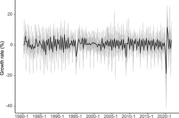
Figure 1 plots the evolution of this variable during our sample period. The black line refers to the national growth rate while the gray lines represent the growth rate of each of the 32 states in the sample. During the major economic crises that Mexico experienced in 1995 and 2009, economic activity decreased by 7.5 and 8.2 per cent, respectively. During the economic recession of 2020, caused by the COVID-19 pandemic, the reduction was significantly larger (20.1 per cent). The growth of economic activity varies substantially at the state level. For example, in 2020, the largest decrease in quarterly economic activity was observed in the spring quarter of 2020 in the state of Quintana Roo (−41.2 per cent), a major touristic destination located in the southeast of Mexico, greatly affected by the social mobility restrictions associated with the COVID-19 pandemic. On the other hand, the largest increase in quarterly economic activity was observed during the summer quarter of 2020 in the state of Zacatecas (26.1 per cent) and is associated with the posterior recovery of the economy following the start of the COVID-19 pandemic. The ITAEE growth rate closely reflects the growth of the state economy when the latter is measured by the gross state domestic product (GSDP) annual growth rate (see figure A1 in the online appendix).
ITAEE quarterly growth rate, 1980–2021.
Note: The black line identifies the national growth rate while the gray lines depict the growth rate in each of the 32 Mexican states.
Source: Own elaboration based on data from INEGI.

Figure 1 Long description
The graph displays ITAEE quarterly growth rates from 1980 to 2021. The vertical axis represents growth rate in percent, ranging from minus 40 to 20. The horizontal axis shows time from 1980 dash 1 to 2020 dash 1. The black line represents the national growth rate, while the gray lines depict growth rates for each of the 32 Mexican states. The national line is smoother, oscillating around 0 percent, with notable peaks and troughs. Around 2020, the national line shows a sharp drop followed by a rebound. The state lines exhibit more volatility, with frequent fluctuations and a cluster of extreme values near 2020. The graph highlights differences in economic activity between the national average and individual states, particularly during major events like the 2020 recession. The thicker black line distinguishes the national data, while thinner gray lines represent state data. The purpose is to illustrate variations in economic growth across Mexico over time.
2.2 Weather data
Monthly weather data for the period 1980–2021 was obtained from DAYMET (Thornton et al., Reference Thornton, Shrestha, Wei, Thornton, Kao and Wilson2022) which provides gridded estimates of monthly average maximum and minimum temperature as well as accumulated precipitation at a 1 km × 1 km spatial resolution. Average monthly temperature results from averaging maximum and minimum temperature. Monthly weather variables are first aggregated to the municipality level by averaging grid cells contained within municipality boundariesFootnote 4 and then aggregated to the state level using a population-weighted average (Burke et al., Reference Burke, Hsiang and Miguel2015).Footnote 5 This procedure assigns higher weights to more populated municipalities. Lastly, monthly weather variables are aggregated to a quarterly basis by averaging monthly temperature and accumulating monthly precipitation.
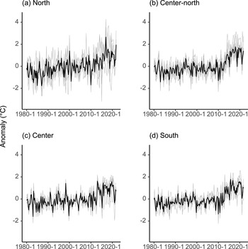
Figure 2 presents the quarterly temperature anomalies observed in the sample period calculated as deviations from the long-term 1980–2021 average, or temperature normal.Footnote 6 In figure 2, states are organized by region. Black lines indicate the regional average anomaly whereas light gray lines identify the anomaly observed in states located within each region (the regional distribution of the 32 Mexican states is shown in figure A2 in the online appendix). Temperature anomalies show large interannual and intra-annual variations. Most of them lie within a 2.0°C band although anomalies outside this range are frequent towards the end of the sample period. The lowest and highest anomalies are −3.2°C and 4.3°C, respectively. Both of these extremes occurred within the last decade and in states located in the North, the region that displays the largest temperature variability.Footnote 7
Quarterly temperature anomalies, 1980–2021.
Note: Black lines refer to the regional average while gray lines represent the temperature anomalies observed in the states located within each region.
Source: Own elaboration based on data from Thornton et al. (Reference Thornton, Shrestha, Wei, Thornton, Kao and Wilson2022).

Figure 2 Long description
The graphs display quarterly temperature anomalies from 1980 to 2021 across four regions: North, Center-north, Center and South. The x-axis represents years from 1980 to 2021 and the y-axis represents anomaly in degree Celsius, ranging from negative 2 to positive 4. Each graph contains multiple thin lines representing individual state anomalies and a thicker black line indicating the regional average anomaly. North: The graph shows fluctuations with a general upward trend, peaking around 4 degrees Celsius in recent years. Center-north: Similar upward trend with less variability, reaching peaks near 3 degrees Celsius. Center: Displays consistent fluctuations with a slight upward trend, peaking around 2 degrees Celsius. South: Shows a gradual increase with peaks near 2 degrees Celsius. Overall, the North region exhibits the largest variability and highest peaks, while other regions show moderate increases over time.
2.3 Summary statistics
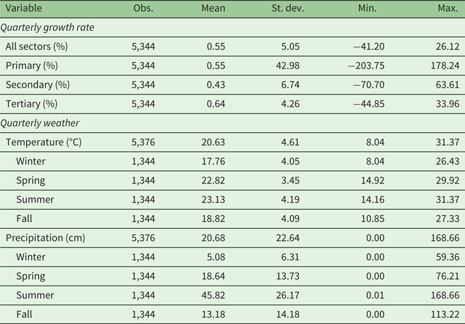
Table 1 presents summary statistics of the working sample at the national level. Growth rates range from −41.2 to 26.1 per cent with an average of 0.55 per cent. The tertiary sector grows, on average, faster than the primary and secondary sectors. The variation observed in economic growth at the sectoral level is even larger than at the aggregate level. The primary sector displays the largest minimum and maximum growth rates with both extreme values seen in the early 1980s. In contrast, for the secondary and tertiary sectors, the minimum and maximum growth rates are associated with the COVID-19 pandemic recession and posterior recovery. Average quarterly temperature ranges from 8.0°C to 31.4°C with a mean of 20.6°C. The spring and summer quarters are the hottest with most of the precipitation being concentrated in the latter.
Sumary statistics of the working sample

Table 1 Long description
The table has six columns: Variable, Obs., Mean, St. dev., Min., Max. Row 1: Quarterly growth rate, blank, blank, blank, blank, blank. Row 2: All sectors (percent) 5,344; 0.55; 5.05; -41.20; 26.12. Row 3: Primary (percent) 5,344; 0.55; 42.98; -203.75; 178.24. Row 4: Secondary (percent) 5,344; 0.43; 6.74; -70.70; 63.61. Row 5: Tertiary (percent) 5,344; 0.64; 4.26; -44.85; 33.96. Row 6: Quarterly weather, blank, blank, blank, blank, blank. Row 7: Temperature (degrees Celsius) 5,376; 20.63; 4.61; 8.04; 31.37. Row 8: Winter 1,344; 17.76; 4.05; 8.04; 26.43. Row 9: Spring 1,344; 22.82; 3.45; 14.92; 29.92. Row 10: Summer 1,344; 23.13; 4.19; 14.16; 31.37. Row 11: Fall 1,344; 18.82; 4.09; 8.05; 27.33. Row 12: Precipitation (centimeters) 5,376; 20.68; 22.64; 0.00; 168.66. Row 13: Winter 1,344; 5.08; 6.31; 0.00; 59.36. Row 14: Spring 1,344; 18.64; 13.73; 0.00; 59.36. Row 15: Summer 1,344; 45.82; 26.17; 0.00; 168.66. Row 16: Fall 1,344; 13.18; 14.18; 0.00; 113.22.
Source: Own elaboration based on data from Thornton et al. (Reference Thornton, Shrestha, Wei, Thornton, Kao and Wilson2022) and INEGI.
3. Empirical strategy
We estimate the functional relationship between temperature and economic growth using a fixed-effects model. Our baseline specification is the following:
 \begin{align} \Delta \textrm{ln}ITAE{E_{it}} & ={\alpha _1}{T_{it}} + {\alpha _2}{T^2}_{it} + {\alpha _3}{P_{it}} + {\alpha _4}{P^2}_{it}\nonumber\\ & \quad + \rho \Delta \textrm{ln}ITAE{E_{i,t - 1}} + {\mu _i} + {\tau _t} + {\vartheta _{ry}} + {\epsilon _{it}}, \end{align}
where the ITAEE growth rate in state i and year-quarter t is modeled as a quadratic function of temperature, T (Burke et al., Reference Burke, Hsiang and Miguel2015). We include as control a quadratic function of precipitation, P, to account for its possible correlation with temperature (Auffhammer et al., Reference Auffhammer, Hsiang, Schlenker and Sobel2013). The estimation also includes one lag of the dependent variable to account for the possibility of autocorrelation in economic growth. The state fixed effects ( ${\mu _i}$) control for all the common time-invariant factors at the state level driving economic activity, while year-by-quarter fixed effects (
 ${\tau _t}$) flexibly control for all the common time-varying factors affecting economic activity across states in the same quarter. The regression also includes region-by-year fixed effects (
 ${\vartheta _{ry}}$) to control for common factors determining growth in states within the same region in a given year.
 ${\epsilon _{it}}$ is the error term. Estimated standard errors are two-way clustered at the state level, to account for serial correlation, and at the region-year level, to account for spatial correlation among states located in the same region-year. In the regressions, observations are weighted by the share of each state in Mexico's total GDP averaged over the 1980–2021 period, an approach also used in Colacito et al. (Reference Colacito, Hoffman and Phan2019) and Jain et al. (Reference Jain, O'Sullivan and Taraz2020). To tease out the differentiated effect of temperature by economic sector, we also estimate equation (1) using the ITAEE growth rate in the primary, secondary and tertiary sectors as dependent variables.
The identifying assumption is that contemporaneous and lagged realizations of weather are stochastic and independent of the rest of the unobserved determinants of economic growth at the state level, conditional on past growth and the fixed effects included in the regression. In the short run, weather anomalies are generally stochastic, unpredictable and unknown to economic agents. Because of this, panel estimates of the effect of weather on economic outcomes have strong causal foundations (Dell et al., Reference Dell, Jones and Olken2014; Blanc and Schlenker, Reference Blanc and Schlenker2017).
4. Results
4.1 The effect of temperature on aggregate economic activity
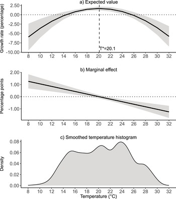
Results are presented graphically in panel (a) of figure 3. Our findings elicit an inverted-U-shaped relationship between temperature and economic activity. Economic growth increases with quarterly average temperature until it reaches a maximum, found to be around an optimal temperature (T*) of 20.1°C at which the expected growth rate is equal to 1.7 per cent.Footnote 8 Once the optimal temperature is exceeded, economic growth decreases. Panel (b) shows that the decrease becomes statistically significant at around 22°C. For example, at 24°C, an increase of 1°C would cause a decrease of −0.41 percentage points in economic growth (see table 1). The decline in economic activity accelerates as quarterly temperature increases. Finally, panel (c) plots the smoothed histogram of quarterly temperature. While it is centered around a mean of 20.6°C, a large proportion of the observations concentrate around 24°C. In fact, half of the Mexican states have average quarterly temperatures larger than the estimated optimum (see figure A6 in the online appendix). In general, temperatures larger than the estimated optimum are observed in 55.3 per cent of the sample. Table A1 (in the online appendix) shows that this result is robust to the inclusion or exclusion of different sets of fixed effects. The inverted-U-shaped relationship remains statistically significant even when the estimation is performed just using cross-sectional variation. The estimated optimal temperature also remains stable and in the vicinity of 20.0°C.
Estimated relationship between temperature and economic growth.
Note: Bands in panel (a) and panel (b) denote confidence intervals at the 95% level.
Source: Own elaboration based on data from INEGI and Thornton et al. (Reference Thornton, Shrestha, Wei, Thornton, Kao and Wilson2022).

Figure 3 Long description
The image A showing Text: a) Expected value. The horizontal axis label: Temperature (degree celsius). The horizontal axis range: 8 to 32. The vertical axis label: Growth rate (percentage). The vertical axis range: negative 10.00 to 2.50. A dotted horizontal reference line is drawn at 0.00. A dashed vertical reference line is drawn at 20. Text near the dashed vertical line: T asterisk equals 20.1. A single curved line rises from about negative 6.0 at 8, crosses 0.00 between 14 and 16, reaches a peak a little above 1.5 around 20, then declines, crossing 0.00 between 24 and 26 and reaches about negative 6.0 at 32. A shaded band surrounds the curved line across the full temperature range. The image B showing Text: b) Marginal effect. The horizontal axis label: Temperature (degree celsius). The horizontal axis range: 8 to 32. The vertical axis label: Percentage points. The vertical axis range: negative 1.00 to 2.00. A dotted horizontal reference line is drawn at 0.00. A single straight line slopes downward from about 1.3 at 8, passes near 0.00 around 20 and reaches about negative 1.2 at 32. A shaded band surrounds the line across the full temperature range. The image C showing Text: c) Smoothed temperature histogram. The horizontal axis label: Temperature (degree celsius). The horizontal axis range: 8 to 32. The vertical axis label: Density. The vertical axis range: 0.00 to 0.08. A filled density curve starts near 0.00 around 8 to 10, rises to about 0.06 around 15 to 16, shows a local high around 20 near 0.07, rises again to a higher peak around 24 near 0.08, then declines to about 0.04 around 27 to 28 and approaches 0.00 by 32.
The non-linear relationship that we find for Mexico is consistent with previous works. However, our estimate of the optimal temperature is larger than what other studies have found. For example, in their global analysis, Burke et al. (Reference Burke, Hsiang and Miguel2015) find that the annual growth of GDP per capita is maximized at 13.0°C. In their analysis for Asia, Lee et al. (Reference Lee, Gaspar and Villaruel2020) conclude that the annual growth of GDP per capita is maximized at 14.2°C. Lastly, in their application for India, Jain et al. (Reference Jain, O'Sullivan and Taraz2020) find an optimal temperature for the annual growth of state GDP equal to 17.6°C. All of these studies rely on annual measures of economic growth and weather. The annual aggregation of these variables possibly attenuates the estimated optimal temperature. We empirically test this by estimating versions of equation (1) in which annual measures of economic growth (constructed using GSDP and ITAEE) and weather are used. Results are presented in table A2 in the online appendix. We also uncover an inverted-U-shaped relationship between annual average temperature and annual economic growth, but the implied optimal temperature is in the vicinity of 18°C. Thus, our use of quarterly data explains the larger optimal temperature that we find. The annual aggregation of both economic growth and weather effectively attenuates the estimated optimal. In our baseline specification, we allow summer (winter) temperatures to be higher (lower) than the annual average. This brings into the estimation a larger source of identifying variation.
4.2 The effect of temperature on economic activity by sector
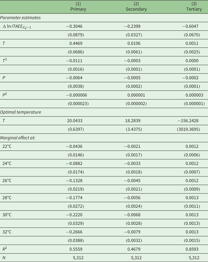
In this section we examine the potential avenues through which temperature affects aggregate economic activity. We do this by estimating our baseline specification using the ITAEE growth rate of the primary, secondary and tertiary sectors as the dependent variable. Results for these three independent estimations are shown in table 2. We find a statistically significant concave relationship between temperature and growth in the primary (column (1)) and secondary (column (2)) sectors with an estimated optimal temperature equal to 20.0°C and 18.3°C, respectively. The same concave relationship is found for the tertiary sector, but the estimated parameters are not statistically significant.
Estimates of the effect of temperature on economic activity by sector

Table 2 Long description
The table has four columns: Column 1, Primary, Secondary and Tertiary. Parameter estimates section. Row: Delta ln ITAEEi,t minus 1. Primary: minus 0.3046 left parenthesis 0.0879 right parenthesis. Secondary: minus 0.2399 left parenthesis 0.0327 right parenthesis. Tertiary: minus 0.6047 left parenthesis 0.0670 right parenthesis. Row: T. Primary: 0.4469 left parenthesis 0.0686 right parenthesis. Secondary: 0.0106 left parenthesis 0.0061 right parenthesis. Tertiary: 0.0011 left parenthesis 0.0025 right parenthesis. Row: T squared. Primary: minus 0.0111 left parenthesis 0.0016 right parenthesis. Secondary: minus 0.0003 left parenthesis 0.0001 right parenthesis. Tertiary: 0.0000 left parenthesis 0.0001 right parenthesis. Row: P. Primary: minus 0.0064 left parenthesis 0.0038 right parenthesis. Secondary: minus 0.0005 left parenthesis 0.0002 right parenthesis. Tertiary: minus 0.0002 left parenthesis 0.0001 right parenthesis. Row: P squared. Primary: minus 0.000006 left parenthesis 0.000023 right parenthesis. Secondary: 0.000001 left parenthesis 0.000002 right parenthesis. Tertiary: 0.000003 left parenthesis 0.000001 right parenthesis. Optimal temperature section. Row: T. Primary: 20.0433 left parenthesis 0.6397 right parenthesis. Secondary: 18.2839 left parenthesis 3.4375 right parenthesis. Tertiary: minus 156.2428 left parenthesis 3019.3695 right parenthesis. Marginal effect at section, with temperatures labeled in degrees Celsius. Row: 22 degrees Celsius. Primary: minus 0.0436 left parenthesis 0.0146 right parenthesis. Secondary: minus 0.0021 left parenthesis 0.0017 right parenthesis. Tertiary: 0.0012 left parenthesis 0.0006 right parenthesis. Row: 24 degrees Celsius. Primary: minus 0.0882 left parenthesis 0.0174 right parenthesis. Secondary: minus 0.0033 left parenthesis 0.0018 right parenthesis. Tertiary: 0.0012 left parenthesis 0.0007 right parenthesis. Row: 26 degrees Celsius. Primary: minus 0.1328 left parenthesis 0.0219 right parenthesis. Secondary: minus 0.0045 left parenthesis 0.0021 right parenthesis. Tertiary: 0.0012 left parenthesis 0.0009 right parenthesis. Row: 28 degrees Celsius. Primary: minus 0.1774 left parenthesis 0.0272 right parenthesis. Secondary: minus 0.0056 left parenthesis 0.0024 right parenthesis. Tertiary: 0.0013 left parenthesis 0.0011 right parenthesis. Row: 30 degrees Celsius. Primary: minus 0.2220 left parenthesis 0.0329 right parenthesis. Secondary: minus 0.0068 left parenthesis 0.0028 right parenthesis. Tertiary: 0.0013 left parenthesis 0.0013 right parenthesis. Row: 32 degrees Celsius. Primary: minus 0.2666 left parenthesis 0.0388 right parenthesis. Secondary: minus 0.0079 left parenthesis 0.0032 right parenthesis. Tertiary: 0.0013 left parenthesis 0.0015 right parenthesis. Model fit section. Row: R squared. Primary: 0.5559. Secondary: 0.4679. Tertiary: 0.8593. Row: N. Primary: 5,312. Secondary: 5,312. Tertiary: 5,312.
Notes: Regressions are weighted by the share of each state in Mexico's total GDP calculated by sector and averaged over the whole 1980–2021. Controls include state, year-by-quarter and year-by-region fixed effects. Standard errors (in parentheses) clustered at the state and region-year level.
Source: Own elaboration based on data from INEGI and Thornton et al. (Reference Thornton, Shrestha, Wei, Thornton, Kao and Wilson2022).
Results for the primary sector are consistent with the abundant empirical evidence documenting a non-linear effect of temperature on agricultural yields (Deschênes and Greenstone, Reference Deschênes and Greenstone2007; Schlenker and Roberts, Reference Schlenker and Roberts2009; Welch et al., Reference Welch, Vincent, Auffhammer, Moya, Dobermann and Dawe2010; Moore and Lobell, Reference Moore and Lobell2014; Burke and Emerick, Reference Burke and Emerick2016; Ortiz-Bobea et al., Reference Ortiz-Bobea, Wang, Carrillo and Ault2019). The general finding of this literature is that hot temperatures are associated with lower agricultural yields. Our results indicate that the growth of the primary sector slows down rapidly once temperature exceeds the optimal level. For example, at 24°C, the reduction in quarterly economic growth is equal to 8.8 percentage points. Precipitation does not have a direct effect on the growth rate of the primary sector. We attribute this result to the fact that the ITAEE growth rate of the primary sector reflects its aggregate performance, merging rainfed and irrigated agriculture together with other primary activities. Such aggregation could explain the noisy estimate that we get for precipitation, but previous applications have documented its importance, especially for rainfed agriculture (Schlenker and Roberts, Reference Schlenker and Roberts2009).
Results for the secondary sector are also consistent with findings from related literature. In their analysis for the US, Graff and Neidell (Reference Graff Zivin and Neidell2014) conclude that high temperatures reduce labor time in industries with heavy exposure to weather such as mining and construction. Similarly, for the Indian manufacturing sector, Somanathan et al. (Reference Somanathan, Somanathan, Sudarshan and Tewari2021) document a reduction in worker productivity and a fall of about 2.0 per cent in plant output caused by high temperatures. According to our estimates, at 24°C, an increase of 1°C in average quarterly temperature would decrease quarterly economic growth in the secondary sector by 0.33 percentage points.
Our lack of results for the tertiary sector could be due to aggregation as ITAEE lumps together the economic performance of several tertiary activities (commerce, transportation, information, financial services, real estate and other services). Previous applications relying on more disaggregated data have documented a negative effect of hotter temperatures in the economic growth of activities such as retail, wholesale, real estate, insurance services and food and drinking services (Colacito et al., Reference Colacito, Hoffman and Phan2019).
4.3 Robustness
When aggregating weather from the municipal to the state level, an alternative is to weight weather based on the share that each municipality represents in the total area of the state. This approach assigns larger weights to large municipalities and accounts for cases where economic activity is more spread out in a municipality. Area-weighted weather has also been used in previous studies (Colacito et al., Reference Colacito, Hoffman and Phan2019; Jain et al., Reference Jain, O'Sullivan and Taraz2020). Columns (1) to (4) of table A3 in the online appendix present results when area-weighted weather is used. The parameter estimates, the implied optimal temperatures and their statistical significance are similar to those of our baseline specification. In columns (5) to (8) of table A3 in the online appendix, we show results obtained when using unweighted weather, that is, weather is aggregated to the state level by taking a simple average of municipal weather. This procedure gives the same importance to all the municipalities regardless of their population or size. Results remain robust. Thus, the weighting procedure to aggregate weather from the municipal to the state level is not driving our results.
In a final robustness test, we evaluate the possibility of Nickel bias which may arise because our regressions include a lag of the dependent variable as a regressor (Nickel, Reference Nickel1981).Footnote 9 Previous works have shown that in the context of long panel data, the fixed-effects estimator is consistent (Anderson and Hsiao, Reference Anderson and Hsiao1981; Nickel, Reference Nickel1981) and its asymptotic bias goes to zero as long as the number of periods (T) is larger than the number of panels (N) (Alvarez and Arellano, Reference Alvarez and Arellano2003). In our setting, T = 168 quarters and N = 32 states, thus, Nickell bias is not likely to be an issue. Table A4 in the online appendix offers reassuring evidence by presenting results from regressions in which the lag of the dependent variable is not included as a regressor. The parameter estimates and the implied optimal temperatures display minor changes compared to our baseline estimates.
5. Heterogeneity analysis
In this section, we delve into the heterogeneity of our results. For this, we estimate different versions of equation (1) in which states are classified into mutually exclusive groups. We test for heterogenous effects of temperature in two different margins: income and agriculture. When classifying states by income, we define groups of Low-Income and High-Income states based on whether their 1980 per capita income is below or above the 1980 median, respectively. Similarly, when classifying states by agriculture, we define Low-Agriculture and High-Agriculture states based on whether their 1980 share of agricultural GSDP in Mexico's total GDP is below or above the 1980 median share, respectively. We chose to classify states using 1980 as reference because it is the first year in our sample which makes the classification exogenous to subsequent realizations of weather. Equation (1) is estimated for each group independently. Table A5 (in the online appendix) provides a list of the Mexican states classified in each group.
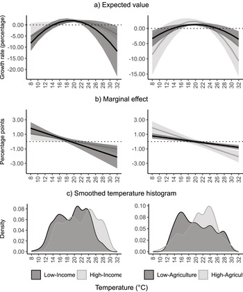
Results are presented graphically in figure 4 (see table A6 in the online appendix for detailed results). We document a statistically significant inverted-U-shaped relationship between economic growth and temperature in both Low-Income and High-Income states (panel (a), left graph). In Low-Income states, the maximum of economic growth is achieved at 19.1°C. In High-Income states, the optimal temperature is found at 20.4°C. As temperature exceeds the optimal level, the fall in economic growth is sharper, on average, for Low-Income states (panel (b), left graph) although the effect is not significantly different from the fall of Low-Income states at all temperatures. On average, Low-Income states tend to experience high temperatures less often than High-Income states (see panel (c), left graph) which may explain the higher sensitivity of their economic growth.
Heterogeneous effect of temperature on economic growth.
Note: Low-Income and High-Income states are classified based on whether their 1980s per capita income is below or above the 1980 median. Low-Agriculture and High-Agriculture states are defined based on whether their 1980s share of agricultural GSDP in total GSDP is below or above the 1980 median share. Regressions are weighted by the share of each state in Mexico's total GDP averaged over the whole 1980–2021 period. Controls include state, year-by-quarter and year-by-region fixed effects. Bands in panels (a) and (b) denote confidence intervals at the 95% level with errors clustered at the state and region-year level.
Source: Own elaboration based on data from INEGI and Thornton et al. (Reference Thornton, Shrestha, Wei, Thornton, Kao and Wilson2022).

Figure 4 Long description
The image A showing a line graph titled a) Expected value. The vertical axis label is Growth rate (percentage), with labeled ticks 0.00, minus 5.00, minus 10.00, minus 15.00, minus 20.00. The horizontal axis shows labeled ticks 8, 10, 12, 14, 16, 18, 20, 22, 24, 26, 28, 30, 32. A dotted horizontal reference line is drawn at 0.00. Two curved lines with shaded bands rise from below 0.00 at 8, reach above 0.00 around 18 to 22, then fall below 0.00 by 32. The image B showing a line graph titled a) Expected value. The vertical axis has labeled ticks 0.00, minus 5.00, minus 10.00, minus 15.00. The horizontal axis shows labeled ticks 8, 10, 12, 14, 16, 18, 20, 22, 24, 26, 28, 30, 32. A dotted horizontal reference line is drawn at 0.00. Two curved lines with shaded bands rise from below 0.00 at 8, reach above 0.00 around 20 to 24, then fall below 0.00 by 32. The image C showing a line graph titled b) Marginal effect. The vertical axis label is Percentage points, with labeled ticks 3.00, 1.00, minus 1.00, minus 3.00. The horizontal axis shows labeled ticks 8, 10, 12, 14, 16, 18, 20, 22, 24, 26, 28, 30, 32. A dotted horizontal reference line is drawn at 0.00. Two downward-sloping lines with shaded bands start above 0.00 near 8 and cross the 0.00 line around 18 to 20, ending below 0.00 near 32. The image D showing a line graph titled b) Marginal effect. The vertical axis has labeled ticks 3.00, 1.00, minus 1.00, minus 3.00. The horizontal axis shows labeled ticks 8, 10, 12, 14, 16, 18, 20, 22, 24, 26, 28, 30, 32. A dotted horizontal reference line is drawn at 0.00. Two downward-sloping lines with shaded bands start above 0.00 near 8 and cross the 0.00 line around 20 to 22, ending below 0.00 near 32. The image E showing a smoothed histogram titled c) Smoothed temperature histogram. The vertical axis label is Density, with labeled ticks 0.02, 0.04, 0.06, 0.08. The horizontal axis label is Temperature (degree celsius), with labeled ticks 8, 10, 12, 14, 16, 18, 20, 22, 24, 26, 28, 30, 32. Two filled density shapes overlap across the temperature range, with higher density between about 12 and 26. The legend labels are Low-Income and High-Income. The image F showing a smoothed histogram titled c) Smoothed temperature histogram. The vertical axis label is Density, with labeled ticks 0.02, 0.05, 0.08, 0.10. The horizontal axis label is Temperature (degree celsius), with labeled ticks 8, 10, 12, 14, 16, 18, 20, 22, 24, 26, 28, 30, 32. Two filled density shapes overlap across the temperature range, with higher density between about 14 and 30. The legend labels are Low-Agriculture and High-Agriculture.
The same non-linear relationship is found when states are divided into Low-Agriculture and High-Agriculture (panel (a), right graph) with estimated optimal temperatures of 19.9°C and 19.5°C, respectively. Additional temperature increases beyond the optimal level cause larger declines in the economic growth of the High-Agriculture states (panel (b), right graph), with the effect being distinguishable from zero at temperatures above 26°C for both groups. This result is consistent with our findings for the primary sector (see table 2) and with the critical role of temperature in agricultural production found in related literature (Schlenker and Roberts, Reference Schlenker and Roberts2009; Burke and Emerick, Reference Burke and Emerick2016; Ortiz-Bobea et al., Reference Ortiz-Bobea, Wang, Carrillo and Ault2019). In the High-Agriculture group, 68.2 per cent of the year-quarter observations fall to the right of the estimated optimum (panel (c), right graph).Footnote 10
Our heterogenous results are consistent with the findings of related literature. Burke et al. (Reference Burke, Hsiang and Miguel2015) find that the sensitivity of the annual growth of income per capita is larger for poor countries compared to rich countries. They also find that the annual growth of agricultural GDP is more sensitive in poor countries compared to rich countries, especially at hot temperatures. Similarly, Jain et al. (Reference Jain, O'Sullivan and Taraz2020) conclude that the annual growth of Indian states decreases at high temperatures with the decrease being larger for states classified as poor or agricultural.
6. Test of adaptation
The average temperature in 2001–2021 was 0.6°C larger than the average temperature of 1981–2000.Footnote 11 This is equivalent to an increase of 0.3°C per decade. If economic agents manage to recognize the sustained increased in temperature over time, they might be able to implement adaptive strategies in order to reduce the sensitivity of their economic activities to hotter temperatures. In this section we investigate if this has been the case for the Mexican economy. If adaptation to climate change has occurred over time, then, we would expect a decreased sensitivity of economic growth to temperature in the later years of our sample. To test for adaptation, we estimate equation (1) independently for 1981–2000 and 2001–2021.
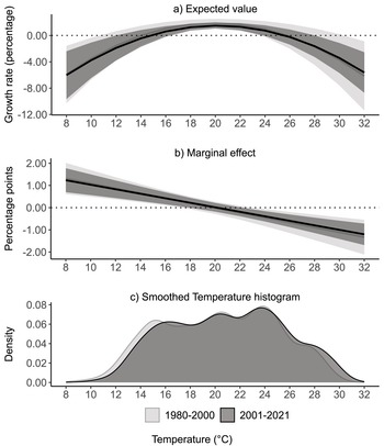
Results of this estimation are presented graphically in figure 5 (see table A9 in the online appendix for detailed regression results). Panel (a) shows that the estimated relationship between temperature and economic growth for 2001–2021 is not statistically different from the relationship for 1980–2000, as confidence intervals overlap over the whole temperature range. Panel (b) shows that the estimated sensitivity of economic growth to temperature, as measured by the marginal effect, is statistically the same in both periods. At high temperatures, the estimated sensitivity using data of the 2001–2021 period is lower on average, which indicates some adaptation, but the reduction is not sufficiently large as to generate a statistically significant difference. The evidence resulting from this analysis suggests that within the 42 years comprising our sample period, adaptation to increasing temperatures has been limited.
Test of adaptation.
Notes: Regressions are weighted by the share of each state in Mexico's total GDP averaged over the whole 1980–2021 period. Controls include state, year-by-quarter and year-by-region fixed effects. Bands in panels (a) and (b) denote confidence intervals at the 95% level with errors clustered at the state and region-year level.
Source: Own elaboration based on data from INEGI and Thornton et al. (Reference Thornton, Shrestha, Wei, Thornton, Kao and Wilson2022).

Figure 5 Long description
The image A showing a) Expected value. The horizontal axis label is Temperature (degree Celsius), with tick labels 8, 10, 12, 14, 16, 18, 20, 22, 24, 26, 28, 30, 32. The vertical axis label is Growth rate (percentage), with tick labels 0.00, minus 4.00, minus 8.00, minus 12.00. A dotted horizontal reference line is drawn at 0.00. Two smooth curves are shown with shaded bands around each curve, corresponding to the two legend periods 1980-2000 and 2001-2021. The curves rise from negative values near Temperature 8 toward values near 0.00 around the mid-range temperatures, then decline to negative values again toward Temperature 32. The image B showing b) Marginal effect. The horizontal axis shows tick labels 8, 10, 12, 14, 16, 18, 20, 22, 24, 26, 28, 30, 32. The vertical axis label is Percentage points, with tick labels 2.00, 1.00, 0.00, minus 1.00, minus 2.00. A dotted horizontal reference line is drawn at 0.00. Two smooth curves are shown with shaded bands around each curve, corresponding to 1980-2000 and 2001-2021. Both curves slope downward from positive values at lower temperatures toward negative values at higher temperatures, crossing the 0.00 reference line around the middle of the temperature range. The image C showing c) Smoothed Temperature histogram. The horizontal axis label is Temperature (degree Celsius), with tick labels 8, 10, 12, 14, 16, 18, 20, 22, 24, 26, 28, 30, 32. The vertical axis label is Density, with tick labels 0.00, 0.02, 0.04, 0.06, 0.08. Two filled density shapes are shown, corresponding to 1980-2000 and 2001-2021. The density is near 0.00 at the lowest and highest temperatures and is higher across mid-range temperatures, with multiple visible humps. Legend labels: 1980-2000 and 2001-2021.
These findings are consistent with Burke et al. (Reference Burke, Hsiang and Miguel2015) and Jain et al. (Reference Jain, O'Sullivan and Taraz2020) who do not find evidence of adaptation to warmer temperature when comparing the effect of temperature on economic growth in two different periods. Our findings also echo the results of Burke and Emerick (Reference Burke and Emerick2016) who do not find evidence of adaptation in the agricultural sector of the USA when comparing the responsiveness of yields to temperature in the short and long run. As done in similar studies, we acknowledge that the absence of adaptation that we find in the Mexican case might be driven by the shortness of our sample period. Economic agents might require more than 21 years to recognize an increasing trend in temperature and adapt accordingly.
7. Implications of climate change for economic growth
In this section, we quantify the likely effect of global warming by simulating the effect of a permanent temperature increase on economic growth.Footnote 12 For this, we rely on temperature projections for 2100 obtained from the Climate Change Knowledge Portal (CCKP) of the World Bank (World Bank, 2023) in turn derived from the latest Coupled Model Inter-comparison Project Phase 6 (CMIP6) which is the foundational data used in the IPPC's Sixth Assessment Report (IPCC, Reference Lee and Romero2023). In the CCKP, temperature projections are available for five Shared Socioeconomic Pathways (SSPs) at the national and subnational levels and with a spatial resolution of 0.25° × 0.25° (25 km × 25 km) (World Bank, 2024).Footnote 13 We use monthly national and state-specific projected temperature changes for 2080–2099 which use 1995–2014 as the baseline period. These projections are derived from a multi-model ensemble mean.Footnote 14 Projected monthly temperature changes were aggregated to a quarterly basis by averaging monthly values.
Figure A7 in the online appendix reports the projected temperature change obtained for every quarter and under each SSP at the national level. Projected temperature increases range from 0.6°C in the fall quarter under SSP1-1.9 to 4.8°C in the summer quarter under SSP5-8.5. The SSP2-4.5 intermediate scenario projects temperature increases between 2°C and 2.5°C in all of the quarters. Within quarters and for a given SSP, projected temperature changes display little variation, with the spring and summer quarters having the largest increases (state level projections are displayed in figure A8 in the online appendix).
Future temperatures for Mexico and its states by the end of the 21st century are calculated as follows. First, a baseline temperature is constructed by calculating a 20-year temperature average using our sample data for 1995–2014, which is the same baseline period as the CMIP6 projections. Then, projected temperatures by 2100 are obtained by adding the projected change in quarterly temperature derived from the CMIP6 projections to the baseline temperature. The estimated change in economic growth rate associated with global warming is equivalent to the difference between the growth rate achieved at projected temperatures and the growth rate achieved at baseline temperatures. This estimation is given by:
 \begin{equation} \Delta GrowthRate = \hat{\alpha}_1\left[{T_F} - {T_B}\right]+ {{\hat{\alpha}}_2} \left[{T^2}_F - {T^2}_B\right],\end{equation}
where TB and TF stand for baseline and future temperature, respectively.  ${\hat{\alpha }_1}$ and
 ${\hat{\alpha }_2}$ are the parameter estimates of our baseline specification (column (1) of table A1 in the online appendix). This calculation is done for every quarter and SSP and for the national and state levels, plugging their respective baseline and future temperatures into equation (2). Equation (2) is also evaluated at the average of the four quarters to estimate an average effect throughout the year. When doing this calculation, we keep precipitation constant at baseline levels as our objective is to isolate the effect of rising temperatures on economic growth.
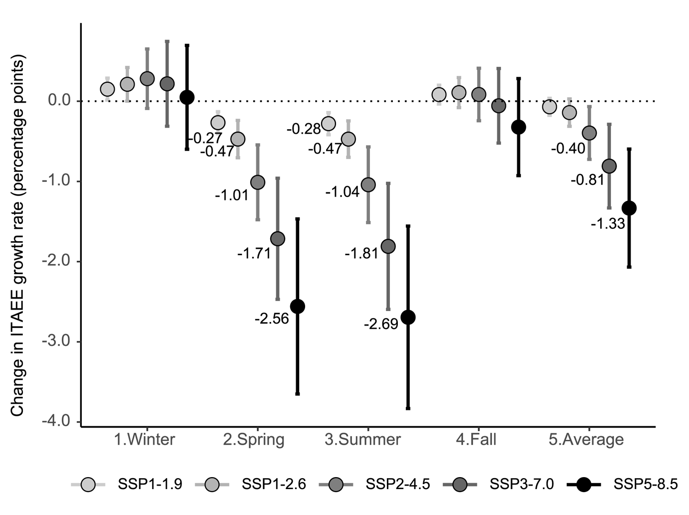
Figure 6 summarizes the projected effect at the national level. There are three main takeaways. First, towards the end of the century, increased temperatures are expected to decrease the economic growth in the spring and summer quarters. The magnitude of the estimated impact increases with the harshness of the SSP. In an intermediate scenario of global warming, the estimated decrease of the growth rate is equal to 1.0 percentage point in the spring and summer quarters. Second, global warming is not expected to affect economic growth in the winter and fall quarters as the estimated impacts are not statistically significant. This result is not surprising given that in Mexico, temperatures during the winter and fall quarters are temperate. Third, the average effect of global warming on economic growth, which is obtained by evaluating equation (2) at the average of the four quarters, ranges from −0.07 to −1.33 percentage points, depending on the severity of the climate change scenario. The intermediate scenario indicates an average loss of 0.40 percentage points in the quarterly growth rate of state economic activity. The magnitude of this effect is not negligible as it represents about two-thirds of the historical average quarterly growth rate (0.55 per cent).Footnote 15
Projected effect of global warming on quarterly economic growth by 2100.
Note: The dotted vertical lines represent confidence intervals at the 95% level. Point estimates are shown only for statistically significant results.
Source: Own elaboration based on data from INEGI and Thornton et al. (Reference Thornton, Shrestha, Wei, Thornton, Kao and Wilson2022).

Figure 6 Long description
Change in ITAEE growth rate (percentage points) A dot chart with vertical error bars and a dotted horizontal reference line at 0.0. The x-axis categories are 1.Winter, 2.Spring, 3.Summer, 4.Fall, 5.Average. The y-axis is labeled “Change in ITAEE growth rate (percentage points)” with tick labels at 0.0, minus 1.0, minus 2.0, minus 3.0 and minus 4.0. A legend below lists five series: SSP1-1.9, SSP1-2.6, SSP2-4.5, SSP3-7.0, SSP5-8.5. For 2.Spring, labeled point values shown are minus 0.27, minus 0.47, minus 1.01, minus 1.71 and minus 2.56, each with a vertical error bar. For 3.Summer, labeled point values shown are minus 0.28, minus 0.47, minus 1.04, minus 1.81 and minus 2.69, each with a vertical error bar. For 5.Average, labeled point values shown are minus 0.40, minus 0.81 and minus 1.33, each with a vertical error bar. For 1.Winter and 4.Fall, multiple circular markers with vertical error bars are plotted near the 0.0 reference line, but no numeric point labels are shown next to those markers.
These results are in line with Colacito et al. (Reference Colacito, Hoffman and Phan2019) who report that the projected increase in temperatures in the US is expected to reduce the annual growth rate of the economy by 0.2–0.4 percentage points by 2100 under a low-emissions scenario. In the US, this result is mainly driven by the negative effect that higher summer temperatures might have on economic activity. We must note, however, that our results are not directly comparable as our measure of economic growth is defined in quarterly terms while theirs is defined in annual terms. Yet, we highlight the relevance of higher summer temperatures in determining future economic losses in both countries. In the Mexican context, higher spring temperatures also contribute to the projected loss in economic growth associated with global warming.
Figure A10 in the online appendix displays the projected effects of global warming on the economic growth at the state level using the SSP2-4.5 intermediate scenario as reference (state results for all scenarios can be found in tables A10–A14 in the online appendix). In the relatively cool winter and fall quarters, several states have positive projections, particularly those located in the temperate central area and some states in the north. In the winter and fall quarters, the negative projections concentrate mainly in coastal states, especially those located in the south of Mexico. In the spring and summer quarters, the economic growth of the vast majority of Mexican states is projected to be negatively affected by rising temperatures. Notably, the economic growth of southern states, already characterized by low economic development (Viesti, Reference Viesti2015), is reduced in all of the quarters. These results are consistent with the findings of Hsiang et al. (Reference Hsiang, Kopp, Jina, Rising, Delgado, Mohan, Rasmussen, Muir-Wood, Wilson, Oppenheimer, Larsen and Houser2017) for the US where the largest GDP losses are also expected to be concentrated in the poorest areas of the country, and with Burke et al. (Reference Burke, Hsiang and Miguel2015) who report that per capita income is projected to fall in poor/hot regions of the world, such as Latin America, while it is projected to increase in rich/cold regions, such as Europe. Our results contribute to the growing empirical evidence of the unequal sharing of the losses associated with global warming.
8. Concluding remarks
In this paper, we estimate the impact of temperature on Mexico's economic growth using 42 years of quarterly panel data at the state level. Our results elicit an inverted-U-shaped relationship between these two variables with an optimal temperature equal to 20.1°C. Temperature affects aggregate economic activity mainly through the effect it has on the growth of the primary and secondary sectors. Our results show that, on average, the economic growth of low-income and high-agriculture states falls more rapidly at high temperatures. They also show that adaptation to global warming in the Mexican economy during the past two decades has been limited. Under an intermediate climate change scenario, we estimate that by 2100, global warming might decrease quarterly economic growth by 0.4 percentage points, on average. Growth losses are expected to be larger during the spring and summer quarters while the economic growth of the fall and winter quarters might not be affected. At the state level, projected losses in economic growth are likely to be concentrated in coastal and southern states.
This study adds another data point regarding the existence of a significant link between temperature and economic growth. Importantly, we do so by relying on quarterly and subnational data. The use of quarterly data brings into the estimations a larger set of identifying variation as opposed to studies relying on annual measures of economic growth and weather which may attenuate the true effect. The use of subnational data allows us to identify specific areas of Mexico whose economic activity may be the most vulnerable to climate change. Our results may facilitate the design and implementation of adaptive strategies to reduce such vulnerability. They indicate that states in the south of Mexico, characterized by low levels of economic development, might be among the most affected since their economic growth may be reduced in every quarter of the year. So, adaptive strategies in these states should be given first priority.
The most effective adaptation strategies may be those directed at the primary and secondary sectors since it is there where we find a significant link. Within the primary sector, there is a lot of room for adaptive measures in agriculture such as the adoption of heat and drought tolerant crop varieties. The expansion of irrigation may also reduce the sensitivity of crops to heat and water stress (Tack et al., Reference Tack, Barkley and Hendricks2017). Within the secondary sector, reducing the exposure of workers to the direct effect of hot temperatures may offset losses in labor productivity and supply. This could be achieved by investing in technologies such as air conditioning (Somanathan et al., Reference Somanathan, Somanathan, Sudarshan and Tewari2021). However, adaptive actions are costly. Thus, increasing access to credit directed at projects related to adaptation to climate change could be another avenue of public policy.
Besides economic growth, global warming could also alter the economic cycle of Mexico. Previous works have documented that economic activity is likely to switch to seasons warming more rapidly (Linsenmeier, Reference Linsenmeier2024). In the Mexican setting, this result implies that future economic production could be reallocated from the winter and fall quarters to the spring and summer quarters (see figure 6). Overall, this could lead to an increased gap in seasonal production and an overall increase in the seasonal economic cycle of Mexico.Footnote 16 The quantification of such an effect is an avenue for future research.
In this article, we have approximated the impact of permanent changes in average temperature on the future economic growth of Mexico. Recent works have concluded that temperature variability reduces economic growth independently and in addition to the effect of changes in average temperature (Kotz et al., Reference Kotz, Wenz, Stechemesser, Kalkuhl and Levermann2021; Linsenmeier, Reference Linsenmeier2023). So, future temperature variability might add to the economic costs of global warming. In the Mexican context, temperature variability is higher in the northern regions. So, while the economic growth of the south might be the most affected by changes in average temperature, the economic growth of the north may be affected by temperature uncertainty to a higher degree. An estimation of the impact of temperature uncertainty on Mexico's economic growth is another avenue for future research.
Like Mexico, other developing warm countries are projected to experience sizable increases in temperature and to bear most of the economic losses attributed to global warming (Burke et al., Reference Burke, Hsiang and Miguel2015; Diffenbaugh and Burke, Reference Diffenbaugh and Burke2019; Acevedo et al., Reference Acevedo, Mrkaic, Novta, Pugacheva and Topalova2020). In isolation, these countries alone can do little to prevent the long-term impact that global warming may have on their economic activity as they contribute much less than developed countries to global CO2 emissions (IPCC, Reference Lee and Romero2023). So, our results stress the need for globally coordinated efforts to limit the temperature increase to a level at which adaptation could still offset economic losses.
Supplementary material
The supplementary material for this article can be found at https://doi.org/10.1017/S1355770X25000026.
Competing interest
None.