1 Introduction
An accurate prediction of aerodynamic noise is an essential requirement to study the physics of sound generation, and to find efficient noise attenuation means. With the increasing power of computers, using numerical method to investigate the sound field is becoming a popular approach. Generally, when attempting to solve an aeroacoustic problem using computational means, a hybrid approach is often used whereby the whole acoustic field is divided into three regions, a source region where the sound is generated, a propagation region and a far-field region where sound radiates (Zhang Reference Zhang2012). The far-field directivity is often of interest to assess the environmental noise impact. At present, a direct calculation of the far-field directivity is still computationally expensive due to high storage and time constraint, despite of the rapidly increasing capacity of the computers. The cost would be too expensive to be useful for practical problems since the grids should be dense enough to reduce numerical dissipation and dispersion. Consequently, a hybrid approach is often adopted that in the near-field sound generation and propagation processes are modelled by high fidelity numerical simulations, while the far-field directivity is extrapolated through alternative acoustic solvers, e.g. based on acoustic analogy theories.
Lighthill (Reference Lighthill1952) proposed the acoustic analogy through a rearrangement of the flow continuity and momentum equations, leading to a linear wave equation with right-hand side quadrupole sources for the density fluctuation defined as
 $\unicode[STIX]{x1D70C}^{\prime }\triangleq \unicode[STIX]{x1D70C}-\unicode[STIX]{x1D70C}_{\infty }$
, where
 $\unicode[STIX]{x1D70C}_{\infty }$
is the density of the far-field medium at rest. Providing that the source terms could be obtained independently such as through a computational fluid dynamics (CFD) computation, Lighthill’s equation is able to describe the sound generation by unsteady flows in an unbounded domain. Subsequently, Curle (Reference Curle1955) extended the original acoustic analogy including the effect of a stationary object, which acts as an acoustical dipole contributed by the surface load. The theory was later extended by Ffowcs Williams & Hawkings (Reference Ffowcs Williams and Hawkings1969) (hereafter FW-H) to allow arbitrary motion for the surface, using the technique of generalised function. As a result, an inhomogeneous wave equation with a volume distributed quadrupole source, two surfaces sources that are monopole and dipole respectively (Brentner & Farassat Reference Brentner and Farassat1998), was obtained. An integral solution to the FW-H equation yields the far-field sound directivity. Additionally, Di Francescantonio (Reference Di Francescantonio1997) derived a sound extrapolation formulation with permeable integration surfaces away from the physical solid boundaries, which allows more practical sources in the integration surface to make the prediction more accurate when the volume integral is ignored (it should be noted that permeable integration surfaces were actually also allowed in Ffowcs Williams & Hawkings’ original paper). The solutions to the FW-H equation by the Green’s function method were given in forms suitable for numerical computations as Farassat formulations 1 and 1A (Farassat & Succi Reference Farassat and Succi1980; Brentner & Farassat Reference Brentner and Farassat1998; Farassat Reference Farassat2007).
Evaluation of the quadrupole sources contributions to noise emission is still computationally expensive since a volume integral over the entire source region is required, even though approximation techniques might be valid in some particular cases (Brentner Reference Brentner1997). Fortunately, in many circumstances its contribution can be ignored since the monopoles and dipoles are the dominant sources (Brentner & Farassat Reference Brentner and Farassat1998). Moreover, errors introduced by neglecting volume sources can be small if the integration surface is large enough such that the sound generation, scattering, refraction, reflection processes are encircled. As a result, far-field sound features could be extrapolated only based on flow variables on the integration surface. This approach works well for pure acoustic radiation problems. However, prediction by this approach can suffer from spurious wave contamination issues when convecting components, not only radiating ones, are collected on the surface. More specifically, the small amplitude fluctuations in a flow field can be decomposed into acoustic, vortical and entropy modes (Kovasznay Reference Kovasznay1953). In cases where the gradient of the background flow is not strong, the vortical and entropy waves would decay slowly and are convected by the background flow. These properties make it difficult to choose an integration surface large enough such that these two modes can vanish completely inside the surface in practical applications such as jet noise prediction (Shur, Spalart & Strelets Reference Shur, Spalart and Strelets2005; Spalart & Shur Reference Spalart and Shur2009; Mendez et al. Reference Mendez, Shoeybi, Lele and Moin2013) where there are convecting density/pressure fluctuations, or in airfoil broadband leading edge noise problems (Gill, Zhang & Joseph Reference Gill, Zhang and Joseph2015) where impinging vortical waves occur. Additionally, in computational aeroacoustics (CAA) computations the grids are often gradually coarsened away from the source region to save computation cost, which requires the integration surfaces be judiciously placed to maintain accuracy. To this end, the integration surface is always expected to be as small as possible provided the essential sound information has been collected. However, spurious waves could be produced when vortical or entropy waves pass across the integration surface; the spurious wave are cancelled if the volume integral is included (Wright & Morfey Reference Wright and Morfey2015). In some previous studies, to avoid the predictions being contaminated by the convected waves while the volume integral is not included, on-body integration surfaces are often adopted (Gill et al. Reference Gill, Zhang and Joseph2015) under the assumption that the noise contribution made by quadrupole volume sources is negligible. In this case, errors can still appear since sound generation (or refraction) by the locally non-uniform flow is discounted; and these errors can be unacceptable if the flow field adjacent to the physical surface varies dramatically. Additionally, the approach is expected to be invalid for cases where there are discontinues in the flow field, e.g. shocks around transonic airfoils (Gill et al. Reference Gill, Zhang, Zhong, Fattah and Angland2016).
Efforts have been made to reduce spurious wave contamination in the presence of convecting disturbances when applying permeable integration surfaces for far-field directivity calculations. Wang, Lele & Moin (Reference Wang, Lele and Moin1996) proposed a correction method to calculate the quadrupole noise due to vortex shedding from an airfoil by assuming that the eddies have a constant speed when they move across the integration surface. A similar idea employing phase shift of the convecting components in the input of the FW-H solver was used by Shur et al. (Reference Shur, Spalart and Strelets2005) for jet noise problems. In numerical implementations, multiple, closely placed integration surfaces are used to record data and the final prediction is an average of the results by those multiple surfaces. The averaging strategy was also adopted by Spalart et al. (Reference Spalart, Shur, Strelets and Travin2011) to predict the far-field noise generated by rudimentary landing gears. The effectiveness was verified by Mendez et al. (Reference Mendez, Shoeybi, Lele and Moin2013), and an expression to estimate the number and positions of the FW-H surfaces for averaging were also given. Additionally, efforts to extend the acoustic analogy were made, e.g. developing formulations in terms of a pressure-like variable (Shur et al.
Reference Shur, Spalart and Strelets2005; Morfey & Wright Reference Morfey and Wright2007) or adopting alternative variables based on some thermodynamic assumptions (Spalart & Shur Reference Spalart and Shur2009). The corresponding volume integral part that would be neglected does not have to be quadrupole in nature, and the results were shown to perform better for the reported jet noise. From another point of view, Obrist & Kleiser (Reference Obrist and Kleiser2007) pointed out that spurious wave generation was related to spectral leakage since the whole domain is sharply truncated by the integration surface. They suggested a smoothly varied spatial window to reduce this truncation error. Moreover, a generalised acoustic analogy that permits window function
 $W(f)$
to be either smoothly or sharply varied was derived by Wright & Morfey (Reference Wright and Morfey2015). In fact, the formulation degraded into the FW-H equation (Ffowcs Williams & Hawkings Reference Ffowcs Williams and Hawkings1969) when
 $W(f)$
is a Heaviside function, and it is equivalent to the averaging approach introduced by Shur et al. (Reference Shur, Spalart and Strelets2005) if
 $W(f)=\sum a_{i}H(f-f_{i})$
is constructed by a series of step functions. It is expected that the performance of this approach would depend on the selection of
 $W(f)$
that is continuous in general, and motion of fluctuations in the transition zone. Its success or failure depends on finding an effective way to optimise the windowing function
 $W(f)$
. Additionally, the time sequence data in the whole transition zone, rather than on a single collection surface must be recorded, which could be impractical. Rahier, Huet & Prieur (Reference Rahier, Huet and Prieur2015) explicitly proved that the spurious wave contamination is caused by neglecting the volume integral terms in the FW-H equations by performing analyses and conducting numerical tests with and without volume integrals. To reduce the spurious wave generation, they proposed a method to replace the neglected volume integral terms by several surface integrals. The effect of the additional terms are approximately equivalent to contribution made by the volume sources in a small region around the integration surface
 $f=0$
(rather than the whole space exterior to the surface). The method is applied to several aeroacoustic problems, and fairly good results are obtained for cases with convecting pressure fluctuations.
In this work, a new sound extrapolation method is introduced for computational aeroacoustic problems, especially for cases where convecting vortical waves are present. The proposed new method is based on the so-called moving medium approach, in which the effect of background flow is explicitly taken into account (Najafi-Yazdi, Brès & Mongeau Reference Najafi-Yazdi, Brès and Mongeau2011). In this approach, a sound wave is received by a stationary observer in a moving medium, which is consistent with the common CFD/CAA computations or wind tunnel tests. In this way, the fluid governing equations are recast to an inhomogeneous convected wave equation other than the classical wave equation. In addition, previous convected acoustic analogy formulations (Gloerfelt, Bailly & Juvé Reference Gloerfelt, Bailly and Juvé2003; Najafi-Yazdi et al.
Reference Najafi-Yazdi, Brès and Mongeau2011; Ghorbaniasl & Lacor Reference Ghorbaniasl and Lacor2012) are developed in the moving frame, and are interchangeable with the original FW-H equation (Ffowcs Williams & Hawkings Reference Ffowcs Williams and Hawkings1969; Brentner & Farassat Reference Brentner and Farassat1998) using coordinate transformation. In all of these methods, the velocity
 $\boldsymbol{u}$
(or the velocity fluctuation
 $\boldsymbol{u}^{\prime }\triangleq \boldsymbol{u}-\boldsymbol{u}_{\infty }$
, the definition of which is different from that adopted in this work), which possibly contains both acoustic and vortical modes, appears in the surface terms. In case that there are convecting vortical waves, spurious wave induced by these source terms can contaminate the sound prediction if the volume integrals are ignored. Efforts are made to address this issue in this work. When deriving the propose method, the fluid dynamic variables are split into steady and fluctuation parts. Then the fluid governing equations can be rewritten in terms of the fluctuation variables assuming the steady background flow is known, and the resultant source terms
 $S_{\unicode[STIX]{x1D70C}}$
,
 $\boldsymbol{S}_{u}$
and
 $S_{p}$
are adopted that alter the acoustic progresses. The equations are further recast to an inhomogeneous wave equation analogously that contains source and volume integral terms. In addition, the two operators
 $\unicode[STIX]{x1D735}\boldsymbol{\cdot }$
and
 $\unicode[STIX]{x2202}_{t}+\boldsymbol{u}_{\infty }\boldsymbol{\cdot }\unicode[STIX]{x1D735}$
are allowed to operate on the velocity fluctuation
 $\boldsymbol{u}^{\prime }$
in the surface terms, and in the expressions of
 $S_{\unicode[STIX]{x1D70C}}$
,
 $\boldsymbol{S}_{u}$
and
 $S_{p}$
. Consequently, spurious wave generation caused by the vortical waves can be filtered or minimised since the vortical waves are divergence free and their motion is simply convected by steady background flow that is usually not strong.
The remaining part of this paper is organised as follows. Section 2 introduces the equation of the proposed sound extrapolation method, and its solution based on the Green’s function method. Section 3 demonstrates sound predictions by the new method, and the results are compared with analytical solutions. Applications to the airfoil leading edge noise problem and comparison with a direct computation are made in §§ 4 and 5 is a summary of this work.
2 Formulations
2.1 Acoustic analogy formulation
In a sound extrapolation method, to obtain an accurate prediction the integration surface is often placed in region where sound propagates, where the flow can be assumed isentropic and inviscid. Additionally, the surface is also required to be away from regions where there might be discontinuities such as shocks that are potential sources. Hence, the following non-conserved form Euler equations are adopted in this work:
 $$\begin{eqnarray}\displaystyle \frac{\unicode[STIX]{x2202}\unicode[STIX]{x1D70C}}{\unicode[STIX]{x2202}t}+\unicode[STIX]{x1D735}\boldsymbol{\cdot }(\unicode[STIX]{x1D70C}\boldsymbol{u})=0,\quad \frac{\unicode[STIX]{x2202}\boldsymbol{u}}{\unicode[STIX]{x2202}t}+\boldsymbol{u}\boldsymbol{\cdot }\unicode[STIX]{x1D735}\boldsymbol{u}+\frac{\unicode[STIX]{x1D735}p}{\unicode[STIX]{x1D70C}}=\mathbf{0},\quad \frac{\unicode[STIX]{x2202}p}{\unicode[STIX]{x2202}t}+\boldsymbol{u}\boldsymbol{\cdot }\unicode[STIX]{x1D735}p+\unicode[STIX]{x1D6FE}p\unicode[STIX]{x1D735}\boldsymbol{\cdot }\boldsymbol{u}=0,\qquad \quad & & \displaystyle\end{eqnarray}$$
where
 $\unicode[STIX]{x1D6FE}$
is the specific heat ratio of gas, and for air
 $\unicode[STIX]{x1D6FE}=1.4$
.
 $\unicode[STIX]{x1D70C}$
,
 $\boldsymbol{u}$
and
 $p$
are the flow density, velocity and pressure respectively. To study the effect of the steady background flow to the behaviour of sound wave, each fluid variable is split into a steady background flow part and an unsteady fluctuation part, i.e.
 $$\begin{eqnarray}\unicode[STIX]{x1D70C}=\unicode[STIX]{x1D70C}_{0}+\unicode[STIX]{x1D70C}^{\prime },\quad \boldsymbol{u}=\boldsymbol{u}_{0}+\boldsymbol{u}^{\prime },\quad p=p_{0}+p^{\prime },\end{eqnarray}$$
where variables with subscript
 $(\cdot )_{0}$
are the steady flow components while
 $(\cdot )^{\prime }$
represent the unsteady fluctuating variables, which is a summation of all the possible acoustic and vortical components. By assuming that the steady background flow also follows the conservation laws, equations (2.1) are exactly cast to the following equations in terms of the fluctuation variables
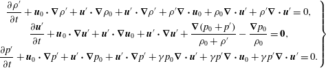 $$\begin{eqnarray}\left.\begin{array}{@{}c@{}}\displaystyle \frac{\unicode[STIX]{x2202}\unicode[STIX]{x1D70C}^{\prime }}{\unicode[STIX]{x2202}t}+\boldsymbol{u}_{0}\boldsymbol{\cdot }\unicode[STIX]{x1D735}\unicode[STIX]{x1D70C}^{\prime }+\boldsymbol{u}^{\prime }\boldsymbol{\cdot }\unicode[STIX]{x1D735}\unicode[STIX]{x1D70C}_{0}+\boldsymbol{u}^{\prime }\boldsymbol{\cdot }\unicode[STIX]{x1D735}\unicode[STIX]{x1D70C}^{\prime }+\unicode[STIX]{x1D70C}^{\prime }\unicode[STIX]{x1D735}\boldsymbol{\cdot }\boldsymbol{u}_{0}+\unicode[STIX]{x1D70C}_{0}\unicode[STIX]{x1D735}\boldsymbol{\cdot }\boldsymbol{u}^{\prime }+\unicode[STIX]{x1D70C}^{\prime }\unicode[STIX]{x1D735}\boldsymbol{\cdot }\boldsymbol{u}^{\prime }=0,\\ \displaystyle \frac{\unicode[STIX]{x2202}\boldsymbol{u}^{\prime }}{\unicode[STIX]{x2202}t}+\boldsymbol{u}_{0}\boldsymbol{\cdot }\unicode[STIX]{x1D735}\boldsymbol{u}^{\prime }+\boldsymbol{u}^{\prime }\boldsymbol{\cdot }\unicode[STIX]{x1D735}\boldsymbol{u}_{0}+\boldsymbol{u}^{\prime }\boldsymbol{\cdot }\unicode[STIX]{x1D735}\boldsymbol{u}^{\prime }+\frac{\unicode[STIX]{x1D735}(p_{0}+p^{\prime })}{\unicode[STIX]{x1D70C}_{0}+\unicode[STIX]{x1D70C}^{\prime }}-\frac{\unicode[STIX]{x1D735}p_{0}}{\unicode[STIX]{x1D70C}_{0}}=\mathbf{0},\\ \displaystyle \frac{\unicode[STIX]{x2202}p^{\prime }}{\unicode[STIX]{x2202}t}+\boldsymbol{u}_{0}\boldsymbol{\cdot }\unicode[STIX]{x1D735}p^{\prime }+\boldsymbol{u}^{\prime }\boldsymbol{\cdot }\unicode[STIX]{x1D735}p_{0}+\boldsymbol{u}^{\prime }\boldsymbol{\cdot }\unicode[STIX]{x1D735}p^{\prime }+\unicode[STIX]{x1D6FE}p_{0}\unicode[STIX]{x1D735}\boldsymbol{\cdot }\boldsymbol{u}^{\prime }+\unicode[STIX]{x1D6FE}p^{\prime }\unicode[STIX]{x1D735}\boldsymbol{\cdot }\boldsymbol{u}_{0}+\unicode[STIX]{x1D6FE}p^{\prime }\unicode[STIX]{x1D735}\boldsymbol{\cdot }\boldsymbol{u}^{\prime }=0.\end{array}\right\}\end{eqnarray}$$
In each of the above equation,
 $\boldsymbol{u}_{0}\boldsymbol{\cdot }\unicode[STIX]{x1D735}(\cdot )^{\prime }$
accounts for the convection effect to the fluctuating variables by the background flow locally. In this work, we consider the situations such that a uniform free stream is introduced at the far-field with free stream pressure
 $p_{\infty }$
, density
 $\unicode[STIX]{x1D70C}_{\infty }$
and velocity
 $\boldsymbol{u}_{\infty }(\neq \mathbf{0})$
, and we intend to study the far-field sound behaviours. The coordinate system adopted is consistent with typical systems in both CFD/CAA and wind tunnel tests. The derivation of the new formulation follows the moving medium approach, and the sound propagation in this case is governed by an inhomogeneous convected wave equation, being different from the original acoustic analogy formulations in which the background flow is at rest (Lighthill Reference Lighthill1952; Ffowcs Williams & Hawkings Reference Ffowcs Williams and Hawkings1969). Therefore, the fluctuation variables are assumed to move in a uniform free stream, while the deviation terms are recast to the right-hand side, i.e. equations (2.3) could be equivalently rearranged to
 $$\begin{eqnarray}\displaystyle & \displaystyle \frac{\unicode[STIX]{x2202}\unicode[STIX]{x1D70C}^{\prime }}{\unicode[STIX]{x2202}t}+\boldsymbol{u}_{\infty }\boldsymbol{\cdot }\unicode[STIX]{x1D735}\unicode[STIX]{x1D70C}^{\prime }+\unicode[STIX]{x1D70C}_{\infty }\unicode[STIX]{x1D735}\boldsymbol{\cdot }\boldsymbol{u}^{\prime }=S_{\unicode[STIX]{x1D70C}}, & \displaystyle\end{eqnarray}$$
 $$\begin{eqnarray}\displaystyle & \displaystyle \frac{\unicode[STIX]{x2202}\boldsymbol{u}^{\prime }}{\unicode[STIX]{x2202}t}+\boldsymbol{u}_{\infty }\boldsymbol{\cdot }\unicode[STIX]{x1D735}\boldsymbol{u}^{\prime }+\frac{\unicode[STIX]{x1D735}p^{\prime }}{\unicode[STIX]{x1D70C}_{\infty }}=\boldsymbol{S}_{u}, & \displaystyle\end{eqnarray}$$
 $$\begin{eqnarray}\displaystyle & \displaystyle \frac{\unicode[STIX]{x2202}p^{\prime }}{\unicode[STIX]{x2202}t}+\boldsymbol{u}_{\infty }\boldsymbol{\cdot }\unicode[STIX]{x1D735}p^{\prime }+\unicode[STIX]{x1D6FE}p_{\infty }\unicode[STIX]{x1D735}\boldsymbol{\cdot }\boldsymbol{u}^{\prime }=S_{p}. & \displaystyle\end{eqnarray}$$
The detailed representations of the terms on the right-hand side are given as
 $$\begin{eqnarray}\displaystyle S_{\unicode[STIX]{x1D70C}} & = & \displaystyle \left(\boldsymbol{u}_{\infty }-\boldsymbol{u}_{0}\right)\boldsymbol{\cdot }\unicode[STIX]{x1D735}\unicode[STIX]{x1D70C}^{\prime }+\left(\unicode[STIX]{x1D70C}_{\infty }-\unicode[STIX]{x1D70C}_{0}\right)\unicode[STIX]{x1D735}\boldsymbol{\cdot }\boldsymbol{u}^{\prime }\nonumber\\ \displaystyle & & \displaystyle -\,\left(\boldsymbol{u}^{\prime }\boldsymbol{\cdot }\unicode[STIX]{x1D735}\unicode[STIX]{x1D70C}_{0}+\unicode[STIX]{x1D70C}^{\prime }\unicode[STIX]{x1D735}\boldsymbol{\cdot }\boldsymbol{u}_{0}\right)-\left(\boldsymbol{u}^{\prime }\boldsymbol{\cdot }\unicode[STIX]{x1D735}\unicode[STIX]{x1D70C}^{\prime }+\unicode[STIX]{x1D70C}^{\prime }\unicode[STIX]{x1D735}\boldsymbol{\cdot }\boldsymbol{u}^{\prime }\right),\end{eqnarray}$$
 $$\begin{eqnarray}\displaystyle \boldsymbol{S}_{u} & = & \displaystyle \left(\boldsymbol{u}_{\infty }-\boldsymbol{u}_{0}\right)\boldsymbol{\cdot }\unicode[STIX]{x1D735}\boldsymbol{u}^{\prime }+\left(\frac{1}{\unicode[STIX]{x1D70C}_{\infty }}-\frac{1}{\unicode[STIX]{x1D70C}_{0}}\right)\unicode[STIX]{x1D735}p^{\prime }\nonumber\\ \displaystyle & & \displaystyle -\,\left(\boldsymbol{u}^{\prime }\boldsymbol{\cdot }\unicode[STIX]{x1D735}\boldsymbol{u}_{0}-\frac{\unicode[STIX]{x1D70C}^{\prime }\unicode[STIX]{x1D735}p_{0}}{\unicode[STIX]{x1D70C}_{0}\unicode[STIX]{x1D70C}}\right)-\left(\boldsymbol{u}^{\prime }\boldsymbol{\cdot }\unicode[STIX]{x1D735}\boldsymbol{u}^{\prime }-\frac{\unicode[STIX]{x1D70C}^{\prime }\unicode[STIX]{x1D735}p^{\prime }}{\unicode[STIX]{x1D70C}_{0}\unicode[STIX]{x1D70C}}\right),\end{eqnarray}$$
 $$\begin{eqnarray}\displaystyle S_{p} & = & \displaystyle \left(\boldsymbol{u}_{\infty }-\boldsymbol{u}_{0}\right)\boldsymbol{\cdot }\unicode[STIX]{x1D735}p^{\prime }+\unicode[STIX]{x1D6FE}\left(p_{\infty }-p_{0}\right)\unicode[STIX]{x1D735}\boldsymbol{\cdot }\boldsymbol{u}^{\prime }\nonumber\\ \displaystyle & & \displaystyle -\,\left(\boldsymbol{u}^{\prime }\boldsymbol{\cdot }\unicode[STIX]{x1D735}p_{0}+\unicode[STIX]{x1D6FE}p^{\prime }\unicode[STIX]{x1D735}\boldsymbol{\cdot }\boldsymbol{u}_{0}\right)-\left(\boldsymbol{u}^{\prime }\boldsymbol{\cdot }\unicode[STIX]{x1D735}p^{\prime }+\unicode[STIX]{x1D6FE}p^{\prime }\unicode[STIX]{x1D735}\boldsymbol{\cdot }\boldsymbol{u}^{\prime }\right).\end{eqnarray}$$
Equations (2.4)–(2.6) describe motion of the fluctuation variables over a free stream medium (denoted by subscript
 $(\cdot )_{\infty }$
), while being driven by additional source terms because of the non-uniform local background flow (denoted by subscript
 $(\cdot )_{0}$
), and nonlinear coupling effects of the fluctuations. To exemplify these effects, the physical meaning of the terms in
 $S_{p}$
will be shown in detail here. The first term
 $(\boldsymbol{u}_{\infty }-\boldsymbol{u}_{0})\boldsymbol{\cdot }\unicode[STIX]{x1D735}p^{\prime }$
represents the difference of the convection effects between the local background flow and the free stream that is adopted to construct the propose convected wave equation. The second term
 $\unicode[STIX]{x1D6FE}(p_{\infty }-p_{0})\unicode[STIX]{x1D735}\boldsymbol{\cdot }\boldsymbol{u}^{\prime }$
represents contribution made by the deviation of the acoustic impedance (defined as
 $Z\triangleq \unicode[STIX]{x1D70C}c=\sqrt{\unicode[STIX]{x1D6FE}\unicode[STIX]{x1D70C}p}\propto p^{(\unicode[STIX]{x1D6FE}+1)/2\unicode[STIX]{x1D6FE}}\propto \unicode[STIX]{x1D70C}^{(\unicode[STIX]{x1D6FE}+1)/2}$
) of both flows. The third term
 $-(\boldsymbol{u}^{\prime }\boldsymbol{\cdot }\unicode[STIX]{x1D735}p_{0}+\unicode[STIX]{x1D6FE}p^{\prime }\unicode[STIX]{x1D735}\boldsymbol{\cdot }\boldsymbol{u}_{0})$
shows the refraction effect caused by the background flow gradient, while the remaining term
 $-(\boldsymbol{u}^{\prime }\boldsymbol{\cdot }\unicode[STIX]{x1D735}p^{\prime }+\unicode[STIX]{x1D6FE}p^{\prime }\unicode[STIX]{x1D735}\boldsymbol{\cdot }\boldsymbol{u})$
corresponds to the nonlinear coupling effect of the fluctuation variables. In an extremely simplified case such that the background flow is exactly the same as the free stream, i.e.
 $(\cdot )_{0}=(\cdot )_{\infty }$
, the source terms
 $S_{\unicode[STIX]{x1D70C}}$
,
 $S_{u}$
and
 $S_{p}$
only contain the nonlinear effects, and they vanish in cases where the fluctuation amplitudes are small. Moreover, the equalities
 $S_{\unicode[STIX]{x1D70C}}=0$
,
 $S_{p}=0$
and
 $\boldsymbol{S}_{u}=-\boldsymbol{u}^{\prime }\boldsymbol{\cdot }\unicode[STIX]{x1D735}\boldsymbol{u}^{\prime }$
hold strictly for simply convected eddies in a uniform flow since
 $p^{\prime }=0$
,
 $\unicode[STIX]{x1D70C}^{\prime }=0$
and
 $\unicode[STIX]{x1D735}\boldsymbol{\cdot }\boldsymbol{u}^{\prime }=0$
.
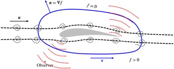
Schematic of the new sound extrapolation method. Physical processes such as sound generation, reflection and refraction are mainly enclosed within the surface
 $f=0$
, while non-radiating vortical waves might be convected across it.

Figure 1 is a schematic of the proposed sound extrapolation method. There might be impinging vortical waves convected by the mean flow and noise is generated in a source region. A permeable integration surface
 $f=0$
is introduced, and the vortical waves might be convected across the surface. The function
 $f$
satisfies
 $|\unicode[STIX]{x1D735}f|=1$
, and in the interior region
 $f<0$
while
 $f>0$
at the outside region. A Heaviside step function
 $H(f)$
is accordingly defined as
 $$\begin{eqnarray}H(f)=\left\{\begin{array}{@{}ll@{}}0, & f<0,\\ 1, & f\geqslant 0.\end{array}\right.\end{eqnarray}$$
The integration surface moves with a velocity
 $\boldsymbol{v}$
, and the outward unit normal vector is
 $\boldsymbol{n}=\unicode[STIX]{x1D735}f$
. The gradient of
 $H(f)$
can be evaluated using the chain rule as
 $$\begin{eqnarray}\frac{\unicode[STIX]{x2202}H(f)}{\unicode[STIX]{x2202}x_{i}}=\unicode[STIX]{x1D6FF}(f)\frac{\unicode[STIX]{x2202}f}{\unicode[STIX]{x2202}x_{i}}=n_{i}\unicode[STIX]{x1D6FF}(f).\end{eqnarray}$$
Here
 $\unicode[STIX]{x1D6FF}(f)$
is the Dirac
 $\unicode[STIX]{x1D6FF}$
function, and the time derivative of
 $H(f)$
is calculated by the following equation
 $$\begin{eqnarray}\frac{\unicode[STIX]{x2202}H}{\unicode[STIX]{x2202}t}+v_{i}\frac{\unicode[STIX]{x2202}H}{\unicode[STIX]{x2202}x_{i}}=0,\quad \Rightarrow \quad \frac{\unicode[STIX]{x2202}H}{\unicode[STIX]{x2202}t}=-\!\boldsymbol{v}\boldsymbol{\cdot }\unicode[STIX]{x1D735}f\unicode[STIX]{x1D6FF}(f)=-v_{n}\unicode[STIX]{x1D6FF}(f).\end{eqnarray}$$
Here we will derive the inhomogeneous convected wave equations in terms of the ‘generalised’ acoustic pressure
 $p^{\prime }H(f)$
since the far-field observing points are usually located outside of the integration surface
 $f=0$
, following similar steps to those adopted by Ffowcs Williams & Hawkings (Reference Ffowcs Williams and Hawkings1969). A combination of (2.6), (2.11) and (2.12) yields
 $$\begin{eqnarray}\displaystyle \left(\frac{\unicode[STIX]{x2202}}{\unicode[STIX]{x2202}t}+\boldsymbol{u}_{\infty }\boldsymbol{\cdot }\unicode[STIX]{x1D735}\right)\{p^{\prime }H(f)\} & = & \displaystyle \unicode[STIX]{x1D6FF}(f)p^{\prime }\left(\boldsymbol{u}_{\infty }-\boldsymbol{v}\right)\boldsymbol{\cdot }\unicode[STIX]{x1D735}f+H(f)\left(\frac{\unicode[STIX]{x2202}}{\unicode[STIX]{x2202}t}+\boldsymbol{u}_{\infty }\boldsymbol{\cdot }\unicode[STIX]{x1D735}\right)p^{\prime }\qquad \nonumber\\ \displaystyle & = & \displaystyle \unicode[STIX]{x1D6FF}(f)p^{\prime }\left(\boldsymbol{u}_{\infty }-\boldsymbol{v}\right)\boldsymbol{\cdot }\unicode[STIX]{x1D735}f+H(f)\{S_{p}-\unicode[STIX]{x1D6FE}p_{\infty }\unicode[STIX]{x1D735}\boldsymbol{\cdot }\boldsymbol{u}^{\prime }\}.\qquad\end{eqnarray}$$
Similarly, starting from the perturbed momentum equation (2.5) we have
 $$\begin{eqnarray}\frac{\unicode[STIX]{x1D735}(p^{\prime }H)}{\unicode[STIX]{x1D70C}_{\infty }}=H(f)\frac{\unicode[STIX]{x1D735}p^{\prime }}{\unicode[STIX]{x1D70C}_{\infty }}+\unicode[STIX]{x1D6FF}(f)\frac{p^{\prime }\unicode[STIX]{x1D735}f}{\unicode[STIX]{x1D70C}_{\infty }}=\unicode[STIX]{x1D6FF}(f)\frac{p^{\prime }\unicode[STIX]{x1D735}f}{\unicode[STIX]{x1D70C}_{\infty }}+H(f)\left[\boldsymbol{S}_{u}-\left(\frac{\unicode[STIX]{x2202}}{\unicode[STIX]{x2202}t}+\boldsymbol{u}_{\infty }\boldsymbol{\cdot }\unicode[STIX]{x1D735}\right)\boldsymbol{u}^{\prime }\right].\end{eqnarray}$$
Then, by performing
 $(\unicode[STIX]{x2202}/\unicode[STIX]{x2202}t+\boldsymbol{u}_{\infty }\boldsymbol{\cdot }\unicode[STIX]{x1D735})$
(2.13) –
 $\unicode[STIX]{x1D6FE}p_{\infty }\unicode[STIX]{x1D735}\boldsymbol{\cdot }$
(2.14), an inhomogeneous convected wave equation can be obtained as
 $$\begin{eqnarray}\left[\left(\frac{\unicode[STIX]{x2202}}{\unicode[STIX]{x2202}t}+\boldsymbol{u}_{\infty }\boldsymbol{\cdot }\unicode[STIX]{x1D735}\right)^{2}-c_{\infty }^{2}\unicode[STIX]{x1D735}^{2}\right]\{p^{\prime }H(f)\}=H(f)S_{v}+\unicode[STIX]{x1D6FF}(f)S_{m}+\frac{\unicode[STIX]{x2202}}{\unicode[STIX]{x2202}t}[Q\unicode[STIX]{x1D6FF}(f)]+\unicode[STIX]{x1D735}\boldsymbol{\cdot }[\boldsymbol{L}\unicode[STIX]{x1D6FF}(f)],\end{eqnarray}$$
where
 $c_{\infty }=\sqrt{\unicode[STIX]{x1D6FE}p_{\infty }/\unicode[STIX]{x1D70C}_{\infty }}$
is the speed of sound of the ambient flow at far field, and detailed expressions of the right-hand terms are
 $$\begin{eqnarray}\left.\begin{array}{@{}c@{}}\displaystyle \boldsymbol{L}=p^{\prime }[\boldsymbol{u}_{\infty }(\boldsymbol{u}_{\infty }-\boldsymbol{v})\boldsymbol{\cdot }\unicode[STIX]{x1D735}f-c_{\infty }^{2}\unicode[STIX]{x1D735}f],\\ \displaystyle Q=p^{\prime }\left(\boldsymbol{u}_{\infty }-\boldsymbol{v}\right)\boldsymbol{\cdot }\unicode[STIX]{x1D735}f,\quad S_{v}=\frac{\text{D}S_{p}}{\text{D}t}-\unicode[STIX]{x1D6FE}p_{\infty }\unicode[STIX]{x1D735}\boldsymbol{\cdot }\boldsymbol{S}_{u},\\ \displaystyle S_{m}=S_{p}(\boldsymbol{u}_{\infty }-\boldsymbol{v})\boldsymbol{\cdot }\unicode[STIX]{x1D735}f-\unicode[STIX]{x1D6FE}p_{\infty }(\boldsymbol{S}_{u}\boldsymbol{\cdot }\unicode[STIX]{x1D735}f)-\unicode[STIX]{x1D6FE}p_{\infty }\left[(\boldsymbol{u}_{\infty }-\boldsymbol{v})\unicode[STIX]{x1D735}\boldsymbol{\cdot }\boldsymbol{u}^{\prime }-\frac{\text{D}\boldsymbol{u}^{\prime }}{\text{D}t}\right]\boldsymbol{\cdot }\unicode[STIX]{x1D735}f,\end{array}\right\}\end{eqnarray}$$
where the notation
 $\text{D}/\text{D}t=\unicode[STIX]{x2202}/\unicode[STIX]{x2202}t+\boldsymbol{u}_{\infty }\boldsymbol{\cdot }\unicode[STIX]{x1D735}$
is adopted for brevity. It should be noted that (2.15) and (2.16) are obtained by an exact rearrangement of the original fluid dynamic equations, and they are the main contribution of this work. Additionally, as will be shown later,
 $S_{v}$
corresponds to the volume source, which is not quadrupole in character as in the previous formulations (Ffowcs Williams & Hawkings Reference Ffowcs Williams and Hawkings1969; Brentner & Farassat Reference Brentner and Farassat1998; Gloerfelt et al.
Reference Gloerfelt, Bailly and Juvé2003; Najafi-Yazdi et al.
Reference Najafi-Yazdi, Brès and Mongeau2011; Ghorbaniasl & Lacor Reference Ghorbaniasl and Lacor2012). The potential error in the proposed method directly depends on the value of
 $S_{v}$
, if it is neglected in sound extrapolation calculations. However, the value of
 $S_{v}$
, which is calculated based on
 $S_{p}$
and
 $\boldsymbol{S}_{u}$
, could be small in the presence of vortical waves, as mentioned before. In addition, since the operators
 $\unicode[STIX]{x1D735}\boldsymbol{\cdot }$
and
 $\text{D}/\text{D}t$
are allowed to act on the velocity fluctuations
 $\boldsymbol{u}^{\prime }$
in the surface term
 $S_{m}$
, the spurious wave generation can therefore be minimised due to the solenoidal and simple convection properties of the vortical wave, while the acoustic field is preserved. However, it should be noted that if there are convecting pressure or density fluctuations in a turbulent flow, such as vortex shedding from airfoils, spurious waves are expected when they are convected across the integration surface. More specifically, the pressure fluctuation
 $p^{\prime }$
appears in
 $\boldsymbol{L}$
,
 $Q$
,
 $S_{p}$
and
 $\boldsymbol{S}_{u}$
contains convecting components, and will make a contribution to spurious wave generation if the volume integral is ignored.
It should be noted that the procedure to split the fluid variables into non-radiating background flow and fluctuation parts was adopted by Goldstein (Reference Goldstein2003) to derive the ‘generalised acoustic analogy’, and in some following studies (Goldstein Reference Goldstein2005; Sinayoko, Agarwal & Hu Reference Sinayoko, Agarwal and Hu2011). In those works, linearised Navier–Stokes (LNS) equations were obtained in terms of a set of modified fluctuations variables, solutions to which yield the sound field. The generalised acoustic analogy promises to provide accurate prediction for challenging aeroacoustic problems with strong sheared flows (Samanta et al. Reference Samanta, Freund, Wei and Lele2006; Goldstein & Leib Reference Goldstein and Leib2008; Karabasov et al. Reference Karabasov, Afsar, Hynes, Dowling, McMullan, Pokora, Page and McGuirk2010). However, a direct computation is required to solve the corresponding LNS equations, or volume integrals are still needed to estimate the far-field directivities.
2.2 Solution to the new inhomogeneous convected wave equation
It is known that the free space Green’s function for the convected wave equations is (Blokhintzev Reference Blokhintzev1946; Najafi-Yazdi et al. Reference Najafi-Yazdi, Brès and Mongeau2011; Ghorbaniasl & Lacor Reference Ghorbaniasl and Lacor2012)
 $$\begin{eqnarray}G(\boldsymbol{x},\boldsymbol{y};t,\unicode[STIX]{x1D70F})=\frac{\unicode[STIX]{x1D6FF}(g)}{4\unicode[STIX]{x03C0}\mathscr{R}}=\frac{\unicode[STIX]{x1D6FF}(t-\unicode[STIX]{x1D70F}-R/c_{\infty })}{4\unicode[STIX]{x03C0}\mathscr{R}},\end{eqnarray}$$
where
 $\boldsymbol{x}$
and
 $\boldsymbol{y}$
are the coordinates of the observer and source points,
 $t$
and
 $\unicode[STIX]{x1D70F}$
are times at observer and source locations, respectively. The variables
 $\mathscr{R}$
and
 $R$
are defined as
 $$\begin{eqnarray}\mathscr{R}=\frac{1}{\unicode[STIX]{x1D6FC}}\sqrt{r^{2}+(\unicode[STIX]{x1D6FC}\boldsymbol{M}_{\infty }\boldsymbol{\cdot }\boldsymbol{ r})^{2}},\quad R=\unicode[STIX]{x1D6FC}^{2}(\mathscr{R}-\boldsymbol{M}_{\infty }\boldsymbol{\cdot }\boldsymbol{r}),\quad \text{with}~\unicode[STIX]{x1D6FC}^{2}=\frac{1}{\unicode[STIX]{x1D6FD}^{2}}=\frac{1}{1-|\boldsymbol{M}_{\infty }|^{2}},\end{eqnarray}$$
where
 $\boldsymbol{r}=\boldsymbol{x}-\boldsymbol{y}$
and
 $r=|\boldsymbol{r}|$
. The solution to the new inhomogeneous convected wave equation can be obtained in an integral form as
 $$\begin{eqnarray}\displaystyle H(f)p^{\prime }(\boldsymbol{x},t) & = & \displaystyle \int _{-\infty }^{t}\int _{\mathbb{R}^{3}}GS_{v}H(f)\,\text{d}\boldsymbol{y}\,\text{d}\unicode[STIX]{x1D70F}+\int _{-\infty }^{t}\int _{\mathbb{R}^{3}}GS_{m}\unicode[STIX]{x1D6FF}(f)\,\text{d}\boldsymbol{y}\,\text{d}\unicode[STIX]{x1D70F}\nonumber\\ \displaystyle & & \displaystyle +\,\frac{\unicode[STIX]{x2202}}{\unicode[STIX]{x2202}t}\int _{-\infty }^{t}\int _{\mathbb{R}^{3}}GQ\unicode[STIX]{x1D6FF}(f)\,\text{d}\boldsymbol{y}\,\text{d}\unicode[STIX]{x1D70F}+\frac{\unicode[STIX]{x2202}}{\unicode[STIX]{x2202}x_{i}}\int _{-\infty }^{t}\int _{\mathbb{R}^{3}}GL_{i}\unicode[STIX]{x1D6FF}(f)\,\text{d}\boldsymbol{y}\,\text{d}\unicode[STIX]{x1D70F}.\qquad\end{eqnarray}$$
It should be noted that the spatial derivatives
 $\unicode[STIX]{x2202}/\unicode[STIX]{x2202}x_{i}$
are performed with respect to the observer coordinate, a direct evaluation of which can be difficult and inaccurate in practical applications, and is therefore not desired. Fortunately, the problem could be avoid by the following calculations (similar derivations could also be found in the paper by Ghorbaniasl & Lacor (Reference Ghorbaniasl and Lacor2012), but here they are displayed for completeness). On one hand,
 $$\begin{eqnarray}\frac{\unicode[STIX]{x2202}}{\unicode[STIX]{x2202}x_{i}}\left(\frac{\unicode[STIX]{x1D6FF}(g)}{\mathscr{R}}\right)=\frac{\unicode[STIX]{x2202}g}{\unicode[STIX]{x2202}x_{i}}\frac{\unicode[STIX]{x1D6FF}^{\prime }(g)}{\mathscr{R}}-\frac{\unicode[STIX]{x2202}\mathscr{R}}{\unicode[STIX]{x2202}x_{i}}\frac{\unicode[STIX]{x1D6FF}(g)}{\mathscr{R}^{2}}=-\frac{1}{c_{\infty }}\frac{\tilde{R}_{i}}{\mathscr{R}}\unicode[STIX]{x1D6FF}^{\prime }(g)-\frac{\tilde{\mathscr{R}}_{i}}{\mathscr{R}^{2}}\unicode[STIX]{x1D6FF}(g).\end{eqnarray}$$
Here
 $g=t-\unicode[STIX]{x1D70F}-R/c_{\infty }$
. In the above expression, the derivatives of
 $R$
and
 $\mathscr{R}$
with respect to
 $x_{i}$
could be calculated directly as
 $$\begin{eqnarray}\tilde{\mathscr{R}}_{i}=\frac{\unicode[STIX]{x2202}\mathscr{R}}{\unicode[STIX]{x2202}x_{i}}=\frac{r_{i}+\unicode[STIX]{x1D6FC}^{2}\boldsymbol{M}_{\infty }\boldsymbol{\cdot }\boldsymbol{r}M_{\infty ,i}}{\unicode[STIX]{x1D6FC}^{2}\mathscr{R}},\quad \tilde{R}_{i}=\frac{\unicode[STIX]{x2202}R}{\unicode[STIX]{x2202}x_{i}}=\unicode[STIX]{x1D6FC}^{2}(\tilde{\mathscr{R}}_{i}-M_{\infty ,i}).\end{eqnarray}$$
On the other hand, as
 $\mathscr{R}$
and
 $\tilde{R}_{i}$
are independent of
 $t$
, one has the following relation:
 $$\begin{eqnarray}\frac{\tilde{R}_{i}}{\mathscr{R}}\unicode[STIX]{x1D6FF}^{\prime }(g)=\frac{\unicode[STIX]{x2202}}{\unicode[STIX]{x2202}t}\left(\frac{\tilde{R}_{i}\unicode[STIX]{x1D6FF}(g)}{\mathscr{R}}\right).\end{eqnarray}$$
Hence, calculations of
 $\unicode[STIX]{x2202}/\unicode[STIX]{x2202}x_{i}$
in (2.19) can be exactly evaluated by two computational effective terms
 $$\begin{eqnarray}\frac{\unicode[STIX]{x2202}}{\unicode[STIX]{x2202}x_{i}}\left(\frac{\unicode[STIX]{x1D6FF}(g)}{\mathscr{R}}\right)=-\frac{1}{c_{\infty }}\frac{\unicode[STIX]{x2202}}{\unicode[STIX]{x2202}t}\left(\frac{\tilde{R}_{i}\unicode[STIX]{x1D6FF}(g)}{\mathscr{R}}\right)-\frac{\tilde{\mathscr{R}}_{i}\unicode[STIX]{x1D6FF}(g)}{\mathscr{R}^{2}}.\end{eqnarray}$$
Additionally, the last three volume integral terms in equation (2.19) are reduced to surface integrals on
 $f=0$
because of the delta function
 $\unicode[STIX]{x1D6FF}(f)$
. Equation (2.19) can therefore be written as follows with the volume integral term neglected
 $$\begin{eqnarray}\displaystyle 4\unicode[STIX]{x03C0}H(f)p^{\prime }(\boldsymbol{x},t) & = & \displaystyle \int _{-\infty }^{t}\int _{f=0}\unicode[STIX]{x1D6FF}(g)\left\{\frac{S_{m}(\boldsymbol{y},\unicode[STIX]{x1D70F})}{\mathscr{R}}-\frac{L_{i}(\boldsymbol{y},\unicode[STIX]{x1D70F})\tilde{\mathscr{R}}_{i}}{\mathscr{R}^{2}}\right\}\,\text{d}S(\boldsymbol{y})\,\text{d}\unicode[STIX]{x1D70F}\nonumber\\ \displaystyle & & \displaystyle +\,\frac{\unicode[STIX]{x2202}}{\unicode[STIX]{x2202}t}\int _{-\infty }^{t}\int _{f=0}\unicode[STIX]{x1D6FF}(g)\left\{\frac{Q(\boldsymbol{y},\unicode[STIX]{x1D70F})}{\mathscr{R}}-\frac{L_{i}(\boldsymbol{y},\unicode[STIX]{x1D70F})\tilde{R_{i}}}{c_{\infty }\mathscr{R}}\right\}\,\text{d}S(\boldsymbol{y})\,\text{d}\unicode[STIX]{x1D70F}.\qquad\end{eqnarray}$$
Furthermore, the time integral in (2.24) could be simplified based on the property of the Dirac
 $\unicode[STIX]{x1D6FF}$
function that
 $$\begin{eqnarray}\int _{-\infty }^{t}F(\unicode[STIX]{x1D70F})\unicode[STIX]{x1D6FF}(g)\,\text{d}\unicode[STIX]{x1D70F}=\left[\frac{F(\unicode[STIX]{x1D70F})}{|\unicode[STIX]{x2202}g/\unicode[STIX]{x2202}\unicode[STIX]{x1D70F}|}\right]_{g=0},\end{eqnarray}$$
where
 $F$
is an arbitrary smooth function. The value of
 $\unicode[STIX]{x2202}g/\unicode[STIX]{x2202}\unicode[STIX]{x1D70F}$
can be evaluated as
 $$\begin{eqnarray}\frac{\unicode[STIX]{x2202}g}{\unicode[STIX]{x2202}\unicode[STIX]{x1D70F}}=1+\frac{1}{c_{\infty }}\frac{\unicode[STIX]{x2202}R}{\unicode[STIX]{x2202}\unicode[STIX]{x1D70F}}=1-\frac{1}{c_{\infty }}\frac{\unicode[STIX]{x2202}y_{i}}{\unicode[STIX]{x2202}\unicode[STIX]{x1D70F}}\tilde{R}_{i}=1-M_{i}\tilde{R}_{i}=1-M_{R},\end{eqnarray}$$
where
 $M_{i}=v_{i}/c_{\infty }$
is the Mach number of the surface motion at the ‘emission time’
 $\unicode[STIX]{x1D70F}_{e}=t-R/c_{\infty }$
. Finally, the formulation used for numerical implementation is written as
 $$\begin{eqnarray}\displaystyle 4\unicode[STIX]{x03C0}H(f)p^{\prime }(\boldsymbol{x},t) & = & \displaystyle \int _{f=0}\left[\frac{1}{1-M_{R}}\left(\frac{S_{m}}{\mathscr{R}}-\frac{L_{i}\tilde{\mathscr{R}}_{i}}{\mathscr{R}^{2}}\right)\right]_{\unicode[STIX]{x1D70F}_{e}}\,\text{d}S\nonumber\\ \displaystyle & & \displaystyle +\,\frac{\unicode[STIX]{x2202}}{\unicode[STIX]{x2202}t}\int _{f=0}\left[\frac{1}{1-M_{R}}\left(\frac{Q}{\mathscr{R}}-\frac{L_{i}\tilde{R_{i}}}{c_{\infty }\mathscr{R}}\right)\right]_{\unicode[STIX]{x1D70F}_{e}}\,\text{d}S,\end{eqnarray}$$
where the subscript
 $[\cdot ]_{\unicode[STIX]{x1D70F}_{e}}$
means the values are evaluated at the emission time
 $\unicode[STIX]{x1D70F}_{e}$
for the given
 $\boldsymbol{x}$
,
 $t$
and source point coordinate
 $\boldsymbol{y}$
on integration surface
 $f=0$
.
3 Numerical implementation and verifications
In this section, far-field acoustic computations are performed to verify the proposed method. The required input data are recorded on three-dimensional (3-D), closed and permeable integration surfaces. In the current implementation, the time interval for data recording on the surface
 $f=0$
is
 $\unicode[STIX]{x0394}\unicode[STIX]{x1D70F}$
, and time interval at the observer point is
 $\unicode[STIX]{x0394}t=\unicode[STIX]{x0394}\unicode[STIX]{x1D70F}$
. The time derivative
 $\unicode[STIX]{x2202}/\unicode[STIX]{x2202}t$
in (2.27) is evaluated by a second-order central-difference scheme. The data collection surface
 $f=0$
is at rest in the medium for simplicity, i.e.
 $v_{i}=0$
. Additionally, the observers are also motionless such that the effective acoustic distance
 $R=\unicode[STIX]{x1D6FC}\sqrt{r^{2}+(\unicode[STIX]{x1D6FC}\boldsymbol{M}_{\infty }\boldsymbol{\cdot }\boldsymbol{ r})^{2}}-\unicode[STIX]{x1D6FC}^{2}\boldsymbol{M}_{\infty }\boldsymbol{\cdot }\boldsymbol{r}$
is fixed for any given observer and source points, and the corresponding ‘emission time’
 $\unicode[STIX]{x1D70F}_{e}$
can therefore be easily evaluated.
Predictions by the proposed method are compared with analytical solutions for the following validation and verification cases: (i) an acoustic monopole source radiation in a uniform flow; (ii) a harmonic vortical wave imposed to the velocity field of the point source in a uniform flow; and (iii) a moving monopole in a uniform flow. For these cases, the nonlinear terms are omitted when calculating
 $S_{p}$
and
 $\boldsymbol{S}_{u}$
since the problems are purely linear. The first case is used to verify the numerical implementation, while the second one is used to demonstrate the capacity of proposed method to avoid being contaminated by vortical waves. The last one is employed to show that the method is adequate to predict instantaneous signals accurately.
3.1 Prediction of a pure acoustic monopole in a uniform flow
The first problem is about a stationary acoustic monopole in a uniform background flow, and the Mach number is denoted as
 $\boldsymbol{M}_{\infty }=(M_{\infty },0,0)$
without loss of generality. The source is of single frequency
 $\unicode[STIX]{x1D714}$
, and the velocity potential is (Lockard Reference Lockard2002)
 $$\begin{eqnarray}\unicode[STIX]{x1D719}(\boldsymbol{x},t)=\frac{A_{p}}{4\unicode[STIX]{x03C0}R_{1}}\exp \left[\text{i}\unicode[STIX]{x1D714}\left(t-\frac{R_{2}}{c_{\infty }}\right)\right],\end{eqnarray}$$
where
 $$\begin{eqnarray}\left.\begin{array}{@{}c@{}}\displaystyle R_{1}=\sqrt{(x_{1}-s_{1})^{2}+\unicode[STIX]{x1D6FD}^{2}[(x_{2}-s_{2})^{2}+(x_{3}-s_{3})^{2}]},\quad R_{2}=\frac{R_{1}-M_{\infty }(x_{1}-s_{1})}{\unicode[STIX]{x1D6FD}^{2}},\\ \displaystyle \unicode[STIX]{x1D6FD}^{2}=1-M_{\infty }^{2}.\end{array}\right\}\end{eqnarray}$$
Here the vector
 $\boldsymbol{s}=(s_{1},s_{2},s_{3})$
is the position of the point source. The acoustic pressure
 $p_{a}^{\prime }$
and particle velocity
 $\boldsymbol{u}_{a}^{\prime }$
are determined as
 $$\begin{eqnarray}p_{a}^{\prime }=\unicode[STIX]{x1D70C}_{a}^{\prime }c_{\infty }^{2}=-\unicode[STIX]{x1D70C}_{\infty }\left(\frac{\unicode[STIX]{x2202}}{\unicode[STIX]{x2202}t}+u_{\infty }\frac{\unicode[STIX]{x2202}}{\unicode[STIX]{x2202}x_{1}}\right)\unicode[STIX]{x1D719},\quad \boldsymbol{u}_{a}^{\prime }=\unicode[STIX]{x1D735}\unicode[STIX]{x1D719}(\boldsymbol{x},t).\end{eqnarray}$$
The sound distribution at the observer points can be obtained from (3.1) and (3.3), and is referred as the analytical solution. The exact solution is also used to calculate values of the perturbation variables at the integration surface
 $f=0$
as input of the sound extrapolation solver. The point source is placed at the origin of the coordinate system, and non-dimensional variables are used. The amplitude of the velocity potential is
 $A_{p}=0.001$
, the pulsation frequency is
 $\unicode[STIX]{x1D714}=2\unicode[STIX]{x03C0}$
and results for two Mach numbers
 $M_{\infty }=0.5$
and
 $0.8$
are demonstrated in this work. A closed spherical data collection surface with a radius
 $r_{s}=1$
is adopted. (Note that data collection surfaces with other shapes, e.g. cylindrical, cubic, were also tested and similar results were obtained.) The observers are placed on a circle on the
 $x_{1}{-}x_{2}$
plane with a radius
 $r_{o}=100$
from the origin. In this work, predictions by the method proposed by Najafi-Yazdi et al. (Reference Najafi-Yazdi, Brès and Mongeau2011) that did not consider the vortical wave effect are also implemented, and the results are also included for comparison.
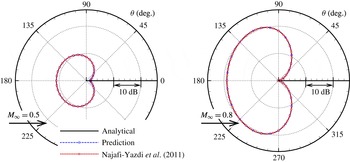
Comparison of the sound pressure level predictions of a monopole in uniform flow by the proposed method and analytical solution (3.3). Predictions by the method of Najafi-Yazdi et al. (Reference Najafi-Yazdi, Brès and Mongeau2011) are also plotted.

Figure 2 shows the sound pressure level (SPL) distribution at the observers. The azimuthal and polar angle of the spherical data collection surface are uniformly divided into 121 and 91 grid points respectively. The sampling frequency is
 $\unicode[STIX]{x0394}f=1/\unicode[STIX]{x0394}\unicode[STIX]{x1D70F}=100\unicode[STIX]{x1D714}/(2\unicode[STIX]{x03C0})$
which has been tested to be large enough to provide accurate calculation of
 $p_{rms}^{\prime }$
. Amplitudes are increased in the upstream direction due to the convection effect, and the increased value would be larger for higher Mach number. It could be seen that both methods are adequate for accurate far-field prediction as shown in the figures. To this end, for problems that only acoustic modes are involved, it is recommended the classical methods (Ffowcs Williams & Hawkings Reference Ffowcs Williams and Hawkings1969; Brentner & Farassat Reference Brentner and Farassat1998; Najafi-Yazdi et al.
Reference Najafi-Yazdi, Brès and Mongeau2011) be used for sound extrapolation since less storage is required to calculate the source terms. In the proposed method there are additional calculations of
 $S_{p}$
and
 $\boldsymbol{S}_{u}$
, and the storage would be doubled compared with the classical approaches. However, the proposed method has advantages in cases there are convecting vortical components, as will be shown in the next section.
3.2 Prediction of acoustic monopole in presence of convecting vortical waves
In this section, the sound field is generated by a fixed monopole in a uniform flow, as in the previous demonstration case, while a harmonic vortical wave that makes no contribution to noise radiation is imposed to the velocity fluctuation field. This case is designed to show the capacity of the proposed method in filtering out the vortical wave while the acoustic property is preserved. On the integration surface
 $f=0$
, the pressure fluctuation (contains only acoustic component) is also calculated by (3.3), while the velocity fluctuation field is evaluated as
 $$\begin{eqnarray}\boldsymbol{u}^{\prime }=\boldsymbol{u}_{a}^{\prime }+\boldsymbol{u}_{v}^{\prime },\quad \text{with}~\boldsymbol{u}_{a}^{\prime }=\unicode[STIX]{x1D735}\unicode[STIX]{x1D719}.\end{eqnarray}$$
Here
 $\boldsymbol{u}_{v}^{\prime }$
is the velocity field corresponding to the impinging harmonic vortical wave that can be written as
 $$\begin{eqnarray}\boldsymbol{u}_{v}^{\prime }=(-k_{2},k_{1})\frac{A_{v}}{\sqrt{k_{1}^{2}+k_{2}^{2}}}\exp [\text{i}k_{1}(x_{1}-u_{\infty }t)+\text{i}k_{2}x_{2}].\end{eqnarray}$$
In this study, configurations of the integration surface and the acoustic wave are the same as in the previous section, i.e.
 $r_{s}=1$
,
 $\unicode[STIX]{x1D714}=2\unicode[STIX]{x03C0}$
and
 $A_{p}=0.001$
. Two different values
 $A_{v}=0.01u_{\infty }$
and
 $A_{v}=0.001u_{\infty }$
are adopted to study the effect of vortical wave strength on the far-field predictions. In addition, wavenumber vectors of the vortical waves are set to be
 $(k_{1},k_{2})=(1,0)$
and
 $(k_{1},k_{2})=(5,0)$
respectively for comparison. The Mach numbers of the uniform flows are
 $M_{\infty }=0.5$
and
 $0.8$
. The sound field distribution should be the same as in the previous case with a pure acoustic monopole since the additional vortical wave is silent.
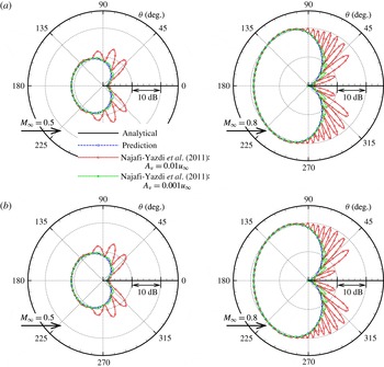
Far-field directivity of a monopole in uniform flows predicted by the new method compared against the analytical solution. Harmonic vortical waves are imposed to the velocity fluctuation field and their wavenumbers are (a)
 $k_{1}=1.0$
,
 $k_{2}=0.0$
and (b)
 $k_{1}=5.0$
and
 $k_{2}=0.0$
. Results calculated by the method of Najafi-Yazdi et al. (Reference Najafi-Yazdi, Brès and Mongeau2011) are also plotted.

Figure 3(a,b) are the far-field directivities predicted by the new method with different Mach numbers of
 $M_{\infty }=0.5$
and
 $M_{\infty }=0.8$
. In all of these demonstrated cases, the predictions match very well with the analytical solutions. Predictions based on the method of Najafi-Yazdi et al. (Reference Najafi-Yazdi, Brès and Mongeau2011) are also displayed, and disagreements are found when compared against the analytical solutions. This is expected as the passage of vortical wave crosses the integration surface, while the volume integrals are discounted. At
 $A_{v}=0.01u_{\infty }$
, it can be seen that with the increase of flow speeds and gust wavenumber
 $|\boldsymbol{k}|$
, more spurious radiation peaks on the directivities appear. When the amplitude of the imposed vortical wave is small, i.e.
 $A_{v}=0.001u_{\infty }$
, the deviations become smaller and the spurious wave contamination issue becomes less significant, but still observable. From these demonstration cases, it can be seen that the new method shows a capacity for accurate sound extrapolation when there are vortical waves in the flow field.
3.3 Prediction of moving acoustic monopole in a uniform flow
In this case, an acoustic point source moves at a speed
 $\boldsymbol{u}_{\infty }$
that is the same as the uniform flow, and the sound propagation follows a convected wave equation. By applying the following space–time transformation,
 $$\begin{eqnarray}\boldsymbol{X}=\boldsymbol{x}-\boldsymbol{u}_{\infty }t,\quad T=t,\quad \Rightarrow \quad \frac{\unicode[STIX]{x2202}}{\unicode[STIX]{x2202}x_{i}}=\frac{\unicode[STIX]{x2202}}{\unicode[STIX]{x2202}X_{i}},\quad \frac{\unicode[STIX]{x2202}}{\unicode[STIX]{x2202}t}=\frac{\unicode[STIX]{x2202}}{\unicode[STIX]{x2202}T}-\boldsymbol{u}_{\infty }\boldsymbol{\cdot }\unicode[STIX]{x1D735},\end{eqnarray}$$
the convected wave equation can be recast to a classical wave equation on the
 $\boldsymbol{X}{-}T$
plane, i.e.
 $$\begin{eqnarray}\left(\frac{\unicode[STIX]{x2202}}{\unicode[STIX]{x2202}t}+\boldsymbol{u}_{\infty }\boldsymbol{\cdot }\unicode[STIX]{x1D735}\right)^{2}\unicode[STIX]{x1D719}-c_{\infty }^{2}\frac{\unicode[STIX]{x2202}^{2}\unicode[STIX]{x1D719}}{\unicode[STIX]{x2202}x_{i}\unicode[STIX]{x2202}x_{i}}=0,\quad \Rightarrow \quad \frac{\unicode[STIX]{x2202}^{2}\unicode[STIX]{x1D719}}{\unicode[STIX]{x2202}T^{2}}-c_{\infty }^{2}\frac{\unicode[STIX]{x2202}^{2}\unicode[STIX]{x1D719}}{\unicode[STIX]{x2202}X_{i}\unicode[STIX]{x2202}X_{i}}=0.\end{eqnarray}$$
Hence, the solution to the problem can be easily obtained as
 $$\begin{eqnarray}p_{a}^{\prime }=-\unicode[STIX]{x1D70C}_{\infty }\frac{\unicode[STIX]{x2202}\unicode[STIX]{x1D719}}{\unicode[STIX]{x2202}T}=-\unicode[STIX]{x1D70C}_{\infty }\left(\frac{\unicode[STIX]{x2202}}{\unicode[STIX]{x2202}t}+\boldsymbol{u}_{\infty }\boldsymbol{\cdot }\unicode[STIX]{x1D735}\right)\unicode[STIX]{x1D719},\quad \boldsymbol{u}_{a}^{\prime }=\unicode[STIX]{x1D735}\unicode[STIX]{x1D719},\end{eqnarray}$$
where
 $$\begin{eqnarray}\unicode[STIX]{x1D719}=\frac{A_{p}}{4\unicode[STIX]{x03C0}\tilde{r}}\exp \left[\text{i}\unicode[STIX]{x1D714}\left(t-\frac{\tilde{r}}{c_{\infty }}\right)\right],\quad \tilde{r}=|\boldsymbol{X}|=|\boldsymbol{x}-\boldsymbol{u}_{\infty }t|.\end{eqnarray}$$
In this work, the radius of the spherical, motionless integration surface is
 $r_{s}=2.0$
, and the Mach number of the uniform flow is
 $M_{\infty }=0.5$
. The monopole source moves inside the integration surface with the speed
 $u_{\infty }$
, its frequency is
 $\unicode[STIX]{x1D714}=4\unicode[STIX]{x03C0}$
and the amplitude is
 $A_{p}=0.001$
. Different observer points are fixed on a circle with a radius
 $r_{o}=20$
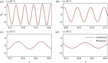
, and the instantaneous pressure signals are recorded. Figure 4 shows the results at four different observer angles
 $\unicode[STIX]{x1D703}=0^{\circ }$
,
 $60^{\circ }$
,
 $120^{\circ }$
and
 $180^{\circ }$
respectively. It could be seen both of the amplitude and frequency of the received sound pressure are altered due to the Doppler effect. For cases with observer angle
 $\unicode[STIX]{x1D703}<90^{\circ }$
, the point source moves towards the observer, as shown in figure 4(a,b), the sound wavelengths are compressed and the amplitudes are amplified gradually. While for cases with
 $\unicode[STIX]{x1D703}>90^{\circ }$
the wavelengths are stretched and the amplitudes are decreased since the point source moves farther away as shown in figure 4(c,d). For all these cases, predictions by the proposed method match well with the analytical solutions.
Comparison of the instantaneous pressure signal of the moving monopole in a
 $M_{\infty }=0.5$
uniform flow by the proposed method and analytical solution. The angle of the observers are: (a)
 $\unicode[STIX]{x1D703}=0^{\circ }$
; (b)
 $\unicode[STIX]{x1D703}=60^{\circ }$
; (c)
 $\unicode[STIX]{x1D703}=120^{\circ }$
; and (d)
 $\unicode[STIX]{x1D703}=180^{\circ }$
.

4 Applications to the airfoil leading edge noise problem
In this section, the new method is applied to numerical simulations of the vortical gust–airfoil leading edge interaction, which is a significant broadband source in turbofan engines or contra-rotating open rotors (CROR) (Amiet Reference Amiet1975; Ganz et al.
Reference Ganz, Joppa, Patten and Scharpf1998; Evers & Peake Reference Evers and Peake2002). Usually, behind the rotating blades there are fully turbulent wakes, which in general are acoustical ineffective but significant noise can be generated when the wakes interact with leading edges of the outlet guide vane in turbofans (or the aft rotors in CRORs). In many numerical studies (Gill et al.
Reference Gill, Zhang and Joseph2015, Reference Gill, Zhang, Zhong, Fattah and Angland2016), divergence-free vortical gusts are introduced into the computational domain to simulate the turbulent fluctuations, while Euler (or linearised Euler) equations are solved to study the sound generation process. In the previous studies, the integral solution to the original FW-H equation (Ffowcs Williams & Hawkings Reference Ffowcs Williams and Hawkings1969; Brentner & Farassat Reference Brentner and Farassat1998) with on-body integration surfaces (e.g. airfoil surface) were often adopted to tackle the spurious wave contamination issue (Gill et al.
Reference Gill, Zhang and Joseph2015). However, inevitable errors are expected in this approach since the influence of non-uniform, near-field flow on sound propagation and generation are not accounted for. In this work, the Euler equations are also solved, and far-field directivities are calculated by (2.27) with various off-body integration surfaces. For comparison, calculations by Farassat formulation 1A (Farassat & Succi Reference Farassat and Succi1980; Brentner & Farassat Reference Brentner and Farassat1998) that are the integral solutions to the original FW-H equation are also performed, and the results are referred to as ‘Farassat-1A’ in the following text. In addition, when evaluating the source terms
 $\boldsymbol{S}_{u}$
and
 $S_{p}$
, nonlinear terms are included since the Euler equations are solved in the simulations.
We also want to highlight the capability of the new method by including cases where locally supersonic flow appears with the increase of flow velocity for the airfoil leading edge problem, with accompanying shocks anchored on the suction surface(s). The on-body integration surface approach is not valid any longer in this case since the local flow varies rapidly in the supersonic zone, and discontinuities due to the shocks can cause additional sound (Gill et al.
Reference Gill, Zhang, Zhong, Fattah and Angland2016). For this reason, far-field predictions using the new method with off-body data collection surfaces that are placed away from the supersonic region are performed in this work. Single frequency harmonic gusts expressed by (3.5) are used as the simplest model of the impinging wakes (Gill et al.
Reference Gill, Zhang and Joseph2015), and only the transverse direction component is considered for simplicity, i.e.
 $k_{2}=0$
. For all cases, the airfoil angle of attack is
 $\unicode[STIX]{x1D6FC}=0^{\circ }$
, the amplitude of the gust (vortical wave) is
 $A_{v}=0.01u_{\infty }$
and the corresponding wavelength of the vortical wave is
 $\unicode[STIX]{x1D706}_{g}=2\unicode[STIX]{x03C0}/k_{1}$
. In the simulations, all variables are non-dimensionalised by using reference length
 $l^{\ast }=c$
that is the airfoil chord length, density
 $\unicode[STIX]{x1D70C}^{\ast }=\unicode[STIX]{x1D70C}_{\infty }$
, speed
 $v^{\ast }=c_{\infty }$
that is the far-field speed of sound, pressure
 $p^{\ast }=\unicode[STIX]{x1D70C}^{\ast }c_{\infty }^{2}$
and time
 $t^{\ast }=l^{\ast }/c_{\infty }$
.
The numerical simulations are performed based on an established CAA code, which has been previously used for various aeroacoustics problems (Zhang et al. Reference Zhang, Chen, Morfey and Nelson2004; Ma & Zhang Reference Ma and Zhang2009; Wang, Hu & Zhang Reference Wang, Hu and Zhang2013; Gill, Zhang & Joseph Reference Gill, Zhang and Joseph2013; Gill et al. Reference Gill, Zhang and Joseph2015). It is able to solve the linearised and full Euler equations, or the Navier–Stokes equations based on high-order finite-difference schemes. Typically, for CAA computations the code employs a fourth-order implicit spatial scheme (Ashcroft & Zhang Reference Ashcroft and Zhang2003) combined with a compact filter with variable cutoff wavenumber to provide high spatial resolution (Bogey & Bailly Reference Bogey and Bailly2004). Additionally, an a priori method is adopted to estimate and improve the grid quality (Fattah, Angland & Zhang Reference Fattah, Angland and Zhang2016). The two-stage fourth-order low-dissipation low-dispersion Runge–Kutta (LDDRK) scheme (Hu, Hussaini & Manthey Reference Hu, Hussaini and Manthey1996) is used for time stepping. Buffer zones are employed for non-reflection boundaries as well as to accommodate impinging vortical waves (Richards et al. Reference Richards, Zhang, Chen and Nelson2004). Additionally, a localised artificial diffusivity scheme (Kawai, Shankar & Lele Reference Kawai, Shankar and Lele2010) is implemented for shock capture. The shock capturing method is an adaptation of the one proposed by Cook (Reference Cook2007) that adds artificial transport coefficients (which are zero for Euler equations) to the viscosity and thermal conductivity of a fluid in regions where are flow discontinuities to remove high wavenumber modes, while the properties in the smooth region are preserved. The discontinuities are identified by using a combination of negative dilatation and a Ducros-type sensor (Ducros et al. Reference Ducros, Ferrand, Nicoud, Weber, Darracq, Gacherieu and Poinsot1999). In addition, the computation grids utilise a sharp trailing edge in this study. Additional numerical treatment is made at the trailing edge point. The flow velocity is forced to be tangential to the surface at most of the airfoil surface, while it is forced to be tangential to the airfoil chord line at the trailing edge point to reduce the numerical errors.
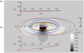
Illustration of the location of the data collection surfaces and distribution of the steady flow pressure (non-dimensional): (a) the result of NACA0002 airfoil; and (b) the result of NACA0012 airfoil. The free stream Mach number is
 $M_{\infty }=0.5$
.

4.1 Predictions of airfoil leading edge noise in subsonic flow
 $M_{\infty }=0.5$

In subsonic flows with free stream Mach number
 $M_{\infty }=0.5$
, 2-D simulations for isolated NACA0012 and NACA0002 airfoils are conducted by solving the Euler equations. A typical calculation can be divided into two stages. At the first stage a steady flow is obtained, and then a single frequency harmonic vortical wave is injected at the upstream boundary that will convect towards and interact with the airfoil leading edge. The distribution of steady flow pressure
 $p_{0}$
fields of the two airfoils are shown in figure 5, as well as the pressure coefficient
 $C_{p}\triangleq (p_{0}-p_{\infty })/(0.5\unicode[STIX]{x1D70C}_{\infty }u_{\infty }^{2})$
along the airfoil surfaces. It can be seen the pressure field around the NACA0002 airfoil is much milder than that of the NACA0012 airfoil. Additionally, geometries of
 $8$
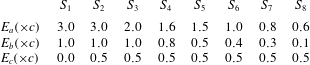
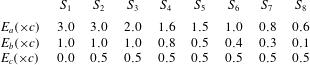
different data collection surfaces are overlapped with the pressure field distributions. The surfaces are elliptic in the 2-D computational domain. The values of the semi-major axis
 $E_{a}$
, semi-minor axis
 $E_{b}$
and centre
 $E_{c}$
are displayed in table 1. In the 2-D computational domain, these off-body surfaces consist of a series of elliptic curves and each of them is uniformly divided into
 $300$
intervals. Additionally, flow information is also recorded on the grid points along the airfoil surfaces for the on-body integral solution using Farassat formulation 1A.
Parameters to determine the data collection surface geometry for the leading edge noise prediction problem. Here
 $c$
is the airfoil chord length.
It should be noted that the sound extrapolation formulation developed in this work is based on the Green’s function in 3-D space, while the simulations are conducted in a 2-D computational domain. To calculate the sound far-field directivity, the simulation data collected on the 2-D curves (parameters of which are given in table 1) are duplicated in the spanwise direction (
 $x_{3}$
) symmetrically with a finite length and the surface integrals are performed on that extended surface
 $\unicode[STIX]{x1D6F4}$
. In addition, it can be proven that the two ends
 $\unicode[STIX]{x1D6F4}^{\pm }$
of the surface make no contribution to far-field sound pressure since the flow velocity in
 $x_{3}$
direction is
 $w=0$
, and the normal vectors of
 $\unicode[STIX]{x1D6F4}^{\pm }$
have opposite directions. As a result, the far-field sound pressure by the proposed sound extrapolation method (or Farassat formulation 1A) with a short span (the length is denoted as
 $L$
) integration surface can be obtained, and is denoted as
 $p_{3D}^{S}$
(or
 $\tilde{p}_{3D}^{S}$
for a specific frequency). In appendix A, the relation between the sound pressure expressed in the 2-D domain
 $\hat{p}_{2D}$
and the predicted data
 $\tilde{p}_{3D}^{S}$
at the far field are derived based on the 2-D–3-D approximation by Oberai, Roknaldin & Hughes (Reference Oberai, Roknaldin and Hughes2002) and the short–long span correction method by Seo & Moon (Reference Seo and Moon2007). For a specific sound frequency (the angular frequency is
 $\unicode[STIX]{x1D714}$
), the relation can be written as
 $$\begin{eqnarray}\hat{p}_{2D}(r,\unicode[STIX]{x1D703},0)={\mathcal{C}}\sqrt{\frac{r}{k}}\frac{(1-M_{\infty }^{2}\sin ^{2}\unicode[STIX]{x1D703})^{1/4}}{L}\tilde{p}_{3D}^{S}(r,\unicode[STIX]{x1D703},0),\quad k=\frac{\unicode[STIX]{x1D714}}{c_{\infty }}.\end{eqnarray}$$
In this work, the 2-D simulation data are duplicated
 $50$
times with a constant interval
 $\unicode[STIX]{x0394}L=0.01c$
to calculate
 $p_{3D}^{S}$
, then the 2-D sound far-field directivity is obtained based on (4.1). It should be noted that the extended span length
 $L=50\unicode[STIX]{x0394}L=0.5c$
has been severely tested in this work such that the predicted directivities by other larger extension length
 $L^{\prime }>L$
are close to each other, which suggests the short–long span correction method by Seo & Moon (Reference Seo and Moon2007) is valid when deriving 4.1. Therefore, for each case the correction factor
 ${\mathcal{C}}\sqrt{r/k}$
can be treated as a constant since the sound field is of single frequency and the radius
 $r=r_{o}$
is a fixed value. Consequently, the shape of the predicted sound directivity will not be influenced if a fixed scale factor is adopted.
Instantaneous pressure
 $p^{\prime }$
distribution of a NACA0012 airfoil in response to a
 $\unicode[STIX]{x1D706}_{g}=0.5c$
vortical gust. The results are obtained numerically by solving the Euler equations. The Mach number is
 $M_{\infty }=0.5$
and the scale is
 $p^{\prime }\in (-10^{-4},10^{-4})$
.

Sound directivity at
 $r=100c$
for the case where a
 $\unicode[STIX]{x1D706}_{g}=0.5c$
harmonic gust interacts with a NACA0012 airfoil. The Mach number is
 $M_{\infty }=0.5$
. The red line with circle symbol (

 $S_{3}$
; the green dashed line (- - -) is the new method on surface
 $S_{1}$
; the blue dash-dotted line (— ⋅ —) the new method on surface
 $S_{2}$
; and the violet dash-dot-dotted (— ⋅ ⋅ —) line is the new method on surface
 $S_{3}$
.

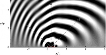
Figure 6 shows an instantaneous distribution of pressure fluctuation
 $p^{\prime }$
for the case where the NACA0012 airfoil responds to a gust with wavelength
 $\unicode[STIX]{x1D706}_{g}=0.5c$
, where
 $c$
is the airfoil chord length, in an
 $M_{\infty }=0.5$
flow. The result is obtained by numerical simulation, and three principle radiation lopes can be identified as indicated by the grey arrows in the figure. Additionally, the far-field sound directivity at
 $r_{o}=100c$
(relative to the airfoil centre) is calculated and the results are shown in figure 7. Data recorded on the on-body surface (airfoil surface) and the off-body surfaces
 $S_{1},S_{2},\ldots ,S_{8}$
are used for sound extrapolation. For the data collection surfaces placed farther away from the airfoil, i.e.
 $S_{1}$
,
 $S_{2}$
and
 $S_{3}$
, the sound directivities obtained by the new method are close to each other, which suggests that the effect of the non-uniform background flow to the sound field have been enclosed in the surfaces. Additionally, predictions by Farassat-1A with the integration surface
 $S_{3}$
are also included in figure 7, yielding multiple peaks and troughs in the directivity as indicted by the black dashed line (- - -). These additional peaks are caused by the passage of the vortical waves across the permeable integration surface
 $S_{3}$
, and are non-physical, as highlighted in the introduction. On the other hand, if Farassat-1A with data collected on the airfoil surface is adopted (

 $120^{\circ }$
and
 $145^{\circ }$
. To study the reason behind this phenomenon, sound directivities with different data collection surfaces located closer to the airfoil surface are calculated by the new method, and the results are shown in figure 8. Here the red line with circular symbols (


 $S_{3}$
. It could be seen that the curves move from
 $S_{3}$
to the on-body results in the observer angle ranges from
 $120^{\circ }$
to
 $145^{\circ }$
, which is consistent with the change of integration surface size. In brief, smaller data collection surfaces will lead to larger prediction errors induced by the background flow non-uniformity, and vice versa. It confirms that the difference between the on-body (


Sound directivity at
 $r=100c$
for the case where a
 $\unicode[STIX]{x1D706}_{g}=0.5c$
harmonic gust interacts with a NACA0012 airfoil. The Mach number is
 $M_{\infty }=0.5$
. The arrow denotes that the integration surface size becomes smaller. The black line with square symbols (- - -) represents
 $S_{3}$
while the red line with circular symbols (

 $\cdots \cdots$
), green dashed (- - -) and black dashed (- - -) lines are results by data collected on surfaces
 $S_{4}$
,
 $S_{5}$
,
 $S_{6}$
,
 $S_{7}$
and
 $S_{8}$
respectively.

To further study the influence of background flow on the far-field directivity, simulations with a thinner airfoil (NACA0002) are conducted, and the steady pressure distribution is demonstrated in figure 5(a). Compared with the NACA0012 case, the flow field varies less rapidly, and the influence of volume sources is therefore relatively smaller. In this case, the analytical solution to the gust–flat plate interaction noise problem (Amiet Reference Amiet1975), which is obtained in the 2-D domain, is calculated for comparison. The far-field directivities predicted by the proposed method with different permeable surfaces (i.e.
 $S_{1},S_{2},\ldots ,S_{8}$
), as well as by Farassat-1A with on-body data (along the NACA0002 airfoil), are shown in figure 9. It can be seen the predicted results by both methods match well with the analytical solution in this case. Additionally, the sound directivity response to NACA0012 by
 $S_{3}$
is also included, and a reduction at low observer angle is found due to the airfoil thickness effect, as investigated in the previous studies (Gill et al.
Reference Gill, Zhang and Joseph2013).
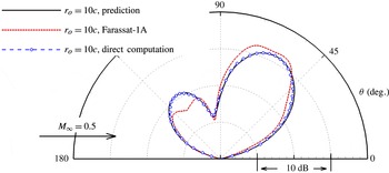
Additionally, comparison of the results predicted by the proposed method and direct computations are conducted to show the accuracy. Sound directivity at
 $r_{o}=10c$
from the airfoil centre is calculated using a large computational domain with a range
 $x\times y=[-25c,25c]\times [-25c,25c]$
. In this case, the NACA0012 at a
 $M_{\infty }=0.5$
flow is subjected to an impinging harmonic vortical wave with a wavelength
 $\unicode[STIX]{x1D706}_{g}=1.0c$
is studied, and only the permeable data collection surface
 $S_{3}$
is used to calculate far-field directivities by both Farassat-1A and the new method proposed in this work. The collected data are also duplicated to the spanwise direction from
 $-0.25c$
to
 $0.25c$
, and the results are shown in figure 10. It can be seen the prediction by the new method matches well with that by direct computation, while a large disagreement induced by the spurious wave contamination is found in the prediction of Farassat-1A method since the volume integral terms are neglected.
Sound directivity at
 $r=100c$
by a
 $\unicode[STIX]{x1D706}_{g}=0.5c$
gust interacting with a NACA0002 airfoil in
 $M_{\infty }=0.5$
flow. The results are: red line with circular symbols (

 $S_{3}$
(


Comparison of the sound directivities predicted by the new method, Farassat-1A and by direct computation at
 $r_{o}=10c$
for a NACA0012 airfoil at
 $M_{\infty }=0.5$
flow. The wavelength of the harmonic gust is
 $\unicode[STIX]{x1D706}_{g}=1.0c$
.

Flow field distributions of a NACA0012 airfoil at
 $M_{\infty }=0.8$
flow: (a) the distribution of Mach number magnitude
 $|\boldsymbol{M}_{0}|$
, and the blue line means the value on the line is
 $|\boldsymbol{M}_{0}|=1.0$
; (b) the distribution of the pressure coefficient
 $C_{p}$
along the airfoil surface.

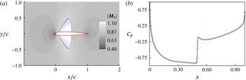
4.2 Predictions of airfoil leading edge noise in transonic flow
$M_{\infty }=0.8$

The gust–leading edge interaction noise problem in a transonic flow was studied by Gill et al. (Reference Gill, Zhang, Zhong, Fattah and Angland2016) to study the acoustic performance of CROR blades operating at high speed, in which case shock waves occur. In this work, a NACA0012 airfoil with zero incidence at Mach number
 $M_{\infty }=0.8$
flow is studied. The magnitude of the steady flow velocity field and pressure coefficient distribution along the airfoil surface (only the suction side results) are shown in figure 11. It can be seen that there is a locally supersonic region on the airfoil surface, and the flow variables experience rapid change in that region. The pressure coefficient along the airfoil surface changes abruptly approximately at half of the airfoil chord, which suggests a terminating shock exists around the airfoil, the flow variables are discontinuous between two sides of shock wave front and the on-body approach cannot be used in this case. To this end, an off-body, permeable, epileptic surface with centre
 $(0.5c,0)$
, semi-major
 $E_{a}=3.0c$
and semi-minor
 $E_{b}=2.0c$
is used to record data for the new method.
Near-field sound distribution of the NACA0012 airfoil interacting with a
 $\unicode[STIX]{x1D706}_{g}=0.5c$
harmonic gust. The Mach number is
 $M_{\infty }=0.8$
. (a) The instantaneous pressure fluctuation
 $p^{\prime }$
distribution and the range of the contours is
 $p^{\prime }\in (-2\times 10^{-4},2\times 10^{-4})$
. (b) The
 $p_{rms}^{\prime }$
distribution and the range of the contours is
 $p_{rms}^{\prime }\in (1\times 10^{-5},3\times 10^{-4})$
.

Far-field sound directivities predicted by the proposed method at two distances
 $r_{o}=100c$
and
 $r_{o}=500c$
. The wavelength of the gust is
 $\unicode[STIX]{x1D706}_{g}=0.5c$
, the flow is transonic and the Mach number is
 $M_{\infty }=0.8$
.

The instantaneous distributions of the fluctuating pressure
 $p^{\prime }$
and root mean square
 $p_{rms}^{\prime }$
of the acoustic response to the gust
 $\unicode[STIX]{x1D706}_{g}=0.5c$
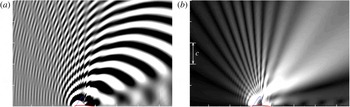
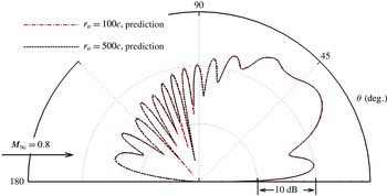
are shown in figure 12(a,b). It can be seen that the acoustic field is significantly altered due to the locally supersonic zone and more interference dips appear (see figure 6 for comparison), especially at the high observation angles, while the downstream directivity seems to be less affected. The far-field directivities at two distances
 $r_{o}=100c$
and
 $500c$
are calculated by the proposed method, and the results are shown in figure 13. It should be noted that the result at
 $r_{o}=500c$
is scaled by the distance from the centre of the airfoil and the two directivities collapse onto each other. Additionally, the interference peaks and dips, as well as the angles are well captured. The detailed physics behind this phenomenon is not the focus of this work, but it can be surmised that challenges exist to study the corresponding far-field characteristic by a direct computation. The acoustic waves are stretched in the downstream region while being compressed in the upstream due to the strong convection of the background flow. As a result, the sound wavelength becomes shorter for high speed flows in the upstream direction. This makes it difficult to directly calculate the far-field sound distribution since the grid should be dense enough, which might be quite unacceptable for short wavelength cases. Nevertheless, we conduct a direct computation with vortical gust wavelength
 $\unicode[STIX]{x1D706}_{g}=1.5c$
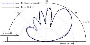
, and the sound directivities are measured by direct computation and by the new method. In this case, the point per wavelength for the upstream propagating acoustic wave is approximately 20 and is found to be sufficient to preserve the accuracy. A comparison of the sound directivities at
 $r_{o}=10c$
by direct computation and by prediction of the new method is shown in figure 14. It can be seen the positions of the radiation peaks and troughs obtained by these two approaches are well matched. By conducting comparisons with the direct computations, it can be concluded the proposed method is adequate to provide accurate predictions for the leading edge noise problems, in both subsonic and transonic cases.
Comparison of the sound directivities predicted by the new method and by direct computation at
 $r_{o}=10c$
. The airfoil is NACA0012, the wavelength of the harmonic gust is
 $\unicode[STIX]{x1D706}_{g}=1.5c$
and the Mach number is
 $M_{\infty }=0.8$
.

5 Summary
Hybrid approaches are often used for computational aeroacoustic problems, i.e. the far-field directivity is extrapolated based on the accurate computation of the near-field fluid or acoustic distributions. This can often be realised by solving an inhomogeneous wave equation (or convected wave equation) obtained from the fluid conservation laws. Generally, the solution contains both volume and surface integrals that correspond to different source terms. In sound extrapolation methods, volume integral terms are often neglected for computational efficiency, which could result in spurious wave contamination when vortical waves are convected across the integration surface.
In this work, a new sound extrapolation method is developed for accurate and effective prediction of far-field acoustic directivity in presence of convecting vortical waves. In derivation of the formulations, the flow variables are split into steady and fluctuation parts, and the fluid governing equations (Euler) are rewritten in terms of the fluctuations variables. Then, they are rearranged to inhomogeneous convected equations utilising the generalised functions, and the source terms correspond to surface and volume integrals respectively in the solution. As for the surface source terms, the operators
 $\unicode[STIX]{x2202}_{t}+\boldsymbol{u}_{\infty }\boldsymbol{\cdot }\unicode[STIX]{x1D735}$
and
 $\unicode[STIX]{x1D735}\boldsymbol{\cdot }$
are allowed to operate on the velocity fluctuations
 $\boldsymbol{u}^{\prime }$
, and the vortical wave is therefore filtered owing to the solenoidal property and it is simply convected by the background flow. In addition, the velocity fluctuations
 $\boldsymbol{u}^{\prime }$
appearing in the volume source term
 $S_{v}$
that quantify the errors the method induced are also filtered by these two operators. Both the spurious wave generation and prediction error induced by the neglected volume source can be quite small for aeroacoustic problems involving convecting vortical waves. The solution to the proposed inhomogeneous convected wave equation is obtained by means of the Green’s function method.
Validation and verification cases are studied with well-defined acoustic sources. It was found that the results obtained by the proposed method match very well with analytical solutions. Moreover, the prediction accuracy of the proposed method is not affected by the presence of vortical waves on the integration surface whilst significant disagreements are observed with previous methods since the volume source terms are not accounted for. Calculations of acoustic far-field directivity of the vortical gust–leading edge interaction problem are also conducted by the proposed method at both subsonic and transonic speeds. Since the integration surfaces can be placed away from the airfoil surface, more of the influence of non-uniform near-field flow to sound emission can be accounted for, making the predictions more accurate than the solution to the original FW-H equation which contains only surface integrals. Additionally, the predictions are also compared with direct computations and the shapes of the directivities match well, adding to our confidence in the new method. It can be concluded the proposed method is adequate for off-body integration surface far-field directivity solutions in the presence of vortical waves by only performing surface integral calculations whilst the spurious noise contamination is greatly suppressed.
However, it should be noted that for more general turbulent flow problems, not only convecting vortical waves, but convecting pressure and density fluctuations may also exist. In these cases, when the volume integral is ignored there could be spurious wave contamination for similar reasons. For this reason, when applying the proposed method to sound extrapolation, the turbulent fluctuation should be dominated by the vortical waves, and severe tests are required before reliable conclusions can be made.
Acknowledgements
S.Z. is supported by the studentship from The Hong Kong University of Science and Technology. The authors would like to acknowledge Dr R. Fattah from The Hong Kong University of Science and Technology and Dr J. Gill from University of Southampton for their helpful discussions. The authors also would like also to show their gratitude to the anonymous reviewers for their constructive suggestions.
Appendix A. Sound directivity correction for 2-D simulations
In this work, we develop a sound extrapolation method based on a 3-D inhomogeneous convected wave equation. On the other hand, when applying the method to predict the gust–airfoil leading edge noise, the simulations are conducted in a 2-D computational domain. In order to calculate the far-field sound directivity, the data collected on a 2-D curve are duplicated in the spanwise direction with a finite length, and then the far-field directivity is obtained through the 3-D sound extrapolation calculation. In this appendix, a detailed explanation about this procedure is made based on the works of Oberai et al. (Reference Oberai, Roknaldin and Hughes2002) and Seo & Moon (Reference Seo and Moon2007).
Firstly, we will revisit the far-field approximation of the sound pressure in 2-D and 3-D domains. The formulation was developed by Oberai et al. (Reference Oberai, Roknaldin and Hughes2002), and here an extension to the uniform mean flow case is made (in the far field, the uniformity property is applicable in many practical situations). Without loss of generality, the uniform mean flow is specified in the
 $x_{1}$
direction and the Mach number is
 $M_{\infty }$
. For a specific frequency, the sound propagation is governed by the convected Helmholtz equation
 $$\begin{eqnarray}\left(\text{i}k+M_{\infty }\frac{\unicode[STIX]{x2202}}{\unicode[STIX]{x2202}x_{1}}\right)^{2}\tilde{p}_{3D}-\left(\frac{\unicode[STIX]{x2202}^{2}}{\unicode[STIX]{x2202}x_{1}^{2}}+\frac{\unicode[STIX]{x2202}^{2}}{\unicode[STIX]{x2202}x_{2}^{2}}+\frac{\unicode[STIX]{x2202}^{2}}{\unicode[STIX]{x2202}x_{3}^{2}}\right)\tilde{p}_{3D}=0\end{eqnarray}$$
where
 $k=\unicode[STIX]{x1D714}/c_{\infty }$
, and
 $\unicode[STIX]{x1D714}$
is the angular frequency of the sound, and the notation
 $\tilde{(\cdot )}$
suggests the sound pressure varies is written in three dimensions and the analysis is performed in the frequency domain. In addition, the far-field condition is required since the sound radiates outwards. By introducing the Prandtl–Glauert transformation
 $$\begin{eqnarray}X_{1}=\frac{x_{1}}{\unicode[STIX]{x1D6FD}},\quad X_{2}=x_{2},\quad X_{3}=x_{3},\quad \unicode[STIX]{x1D6FD}=\sqrt{1-M_{\infty }^{2}},\end{eqnarray}$$
equation (A 1) is transformed into an alternative classical Helmholtz equation in the new coordinate system
 $(X_{1},X_{2},X_{3})$
 $$\begin{eqnarray}\left(\frac{\unicode[STIX]{x2202}^{2}}{\unicode[STIX]{x2202}X_{1}^{2}}+\frac{\unicode[STIX]{x2202}^{2}}{\unicode[STIX]{x2202}X_{2}^{2}}+\frac{\unicode[STIX]{x2202}^{2}}{\unicode[STIX]{x2202}X_{3}^{2}}\right)\tilde{p}_{3D}+k_{\unicode[STIX]{x1D6FD}}^{2}\tilde{p}_{3D}=0,~~~k_{\unicode[STIX]{x1D6FD}}=\frac{k}{\unicode[STIX]{x1D6FD}}.\end{eqnarray}$$
Following similar analysis conducted in Oberai et al. (Reference Oberai, Roknaldin and Hughes2002, pp. 2207–2208), on the
 $X_{3}=0$
plane and under the far-field assumption, the sound pressures in two and three dimensions (for the
 $k_{3}=0$
component) are related by
 $$\begin{eqnarray}\tilde{p}_{3D}(R,\unicode[STIX]{x1D6E9},0)\approx \hat{p}_{2D}(R,\unicode[STIX]{x1D6E9},0)\frac{1+i}{2}\sqrt{\frac{k_{\unicode[STIX]{x1D6FD}}}{\unicode[STIX]{x03C0}R}}\end{eqnarray}$$
where
 $R=(X_{1}^{2}+X_{2}^{2})^{1/2}$
and
 $\unicode[STIX]{x1D6E9}=\tan ^{-1}(X_{2}/X_{1})$
. To study the sound directivity on the
 $x_{1}{-}x_{2}$
plane, the relationship can be explicitly written as
 $$\begin{eqnarray}\left.\frac{\hat{p}_{2D}(r,\unicode[STIX]{x1D703},0)}{\tilde{p}_{3D}(r,\unicode[STIX]{x1D703},0)}\right|_{k_{3}=0}=\frac{2}{1+i}\sqrt{\frac{\unicode[STIX]{x03C0}R}{k_{\unicode[STIX]{x1D6FD}}}}=\frac{2}{1+i}\sqrt{\frac{\unicode[STIX]{x03C0}r}{k}}\left(1-M_{\infty }^{2}\sin ^{2}\unicode[STIX]{x1D703}\right)^{1/4}\end{eqnarray}$$
where
 $r=(x_{1}^{2}+x_{2}^{2})^{1/2}$
and
 $\unicode[STIX]{x1D703}=\tan ^{-1}(x_{2}/x_{1})$
are the radius and observer angles respectively. An additional term
 $(1-M_{\infty }^{2}\sin ^{2}\unicode[STIX]{x1D703})^{1/4}$
is introduced to account for the mean flow effect compared with the results by Oberai et al. (Reference Oberai, Roknaldin and Hughes2002).
It should be noted that the 3-D data
 $\tilde{p}_{3D}$
appearing in (A 5) vary in the range
 $-\infty <x_{3}<\infty$
, or approximately along a long span surface (though the formulation is valid on the
 $x_{3}=0$
plane). However, the predicted sound directivity by the spanwise direction extension can provide far-field prediction
 $\tilde{p}_{3D}^{S}$
only on a finite surface with span length
 $L$
. Fortunately, following the long span body correction method proposed by Seo & Moon (Reference Seo and Moon2007), the predicted data
 $\tilde{p}_{3D}^{S}$
are related with the long span data
 $\tilde{p}_{3D}$
by
 $$\begin{eqnarray}\tilde{p}_{3D}\propto \frac{1}{L}\tilde{p}_{3D}^{S}.\end{eqnarray}$$
It should be noted (A 6) is obtained based on the third condition of (19) of Seo & Moon (Reference Seo and Moon2007). In fact, under the far-field approximation, the phase difference between two segments
 $\unicode[STIX]{x1D709}_{m}$
and
 $\unicode[STIX]{x1D709}_{n}$
(in
 $x_{3}$
direction) on the integration surface to a far-field observer point can be approximately represented as
 $$\begin{eqnarray}\unicode[STIX]{x0394}\unicode[STIX]{x1D719}_{mn}=k\left(\sqrt{r^{2}+\unicode[STIX]{x1D709}_{m}^{2}}-\sqrt{r^{2}+\unicode[STIX]{x1D709}_{n}^{2}}\right)\approx \frac{\unicode[STIX]{x1D709}_{m}^{2}-\unicode[STIX]{x1D709}_{n}^{2}}{(\sqrt{r/k})^{2}},\quad r\gg \unicode[STIX]{x1D709}_{m},\unicode[STIX]{x1D709}_{n}.\end{eqnarray}$$
In this case, the corresponding coherence length
 $L_{c}^{\prime }$
defined in Seo & Moon, (17)’s paper is
 $L_{c}^{\prime }=\sqrt{r/k}$
. This suggests the variables could satisfy that condition since
 $r$
is large under the far-field assumption. As a result, the predicted directivity
 $\tilde{p}_{3D}^{S}$
should be scaled by the extended length
 $L$
in these cases. In summary, the 2-D acoustic far-field directivity (that is desired in this work) and the 3-D predicted result
 $\tilde{p}_{3D}^{S}$
(via the spanwise extension approach) are related as
 $$\begin{eqnarray}\hat{p}_{2D}(r,\unicode[STIX]{x1D703},0;k)\propto \sqrt{\frac{r}{k}}\frac{\left(1-M_{\infty }^{2}\sin ^{2}\unicode[STIX]{x1D703}\right)^{1/4}}{L}\tilde{p}_{3D}^{S}(r,\unicode[STIX]{x1D703},0;k).\end{eqnarray}$$