1. Introduction
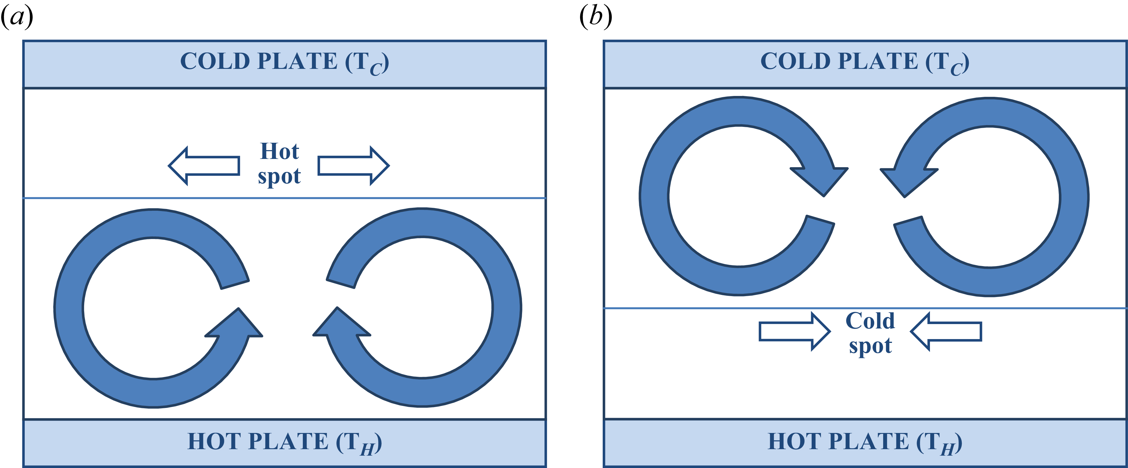
The phenomenon of Rayleigh–Bénard–Marangoni (RBM) convection in multiple fluid layers has attracted broader interest due to its facets of pattern formation (Newell & Whitehead Reference Newell and Whitehead1969) and its relevance in diverse scenarios such as Earth mantle convection (Richter & Johnson Reference Richter and Johnson1974; Busse Reference Busse1981) and liquid encapsulated crystal growth (Johnson Reference Johnson1975; Shen et al. Reference Shen, Neitzel, Jankowski and Mittelmann1990; Zhao et al. Reference Zhao, Wagner, Narayanan and Friedrich1995). The multi-modal interactions between the layers in such systems manifest varied and complex patterns. Zeren & Reynolds (Reference Zeren and Reynolds1972) classified the manifestations into three possible modes, viz. interfacial-tension-gradient-dominated mode, buoyancy-dominated mode and surface-deflection-dominated mode (Zhao et al. Reference Zhao, Wagner, Narayanan and Friedrich1995). Among them, the buoyancy-dominated mode can be further classified based on the number of layers that undergo primary excitation. When the convection is dominant in only one of the layers, it is commonly referred to as the `dragging mode’ (Johnson & Narayanan Reference Johnson and Narayanan1997), wherein the other passive layers are driven by the continuity of velocity and shear stress at the fluid interfaces. When more than one layer undergoes primary excitation, two distinct non-oscillatory modes can occur: the mechanical coupling (MC, counter-rotating rolls) mode and the thermal coupling (TC, co-rotating rolls) mode. For specific fluid properties and system configurations, one can also observe overstability or oscillatory patterns (Rasenat, Busse & Rehberg Reference Rasenat, Busse and Rehberg1989) that occur when there is competition between a minimum of two modes, i.e. between a bulk mode and an interfacial mode or between two bulk modes. For example, in a simple two-layer Rayleigh-Bénard (RB) system, the overstability manifests as cyclic transitions between MC and TC states (Colinet & Legros Reference Colinet and Legros1994). When the system is in the MC state, the diffusion of thermal perturbations across the interface, along with buoyancy effects, causes roll inversion and a subsequent transition to a TC state. However, such a TC state is short-lived as the system cannot sustain the viscous dissipation of the small counter-rotating (buffer) rolls that are formed to enforce mechanical continuity near the interface. Thus, the buffer roll transiently grows and results in the reformation of the MC state, which again transitions to a TC state and, eventually, perpetuates an oscillatory onset of convection. Linear stability analysis of Renardy & Renardy (Reference Renardy and Renardy1985) showed that for such repeated transitions to occur, i.e. for the system to be non-self-adjoint and exhibit Hopf bifurcation, it would require certain favourable property ratio combinations. Renardy (Reference Renardy1996) showed that for infinite Prandtl number and pure buoyancy-driven convection, the system would be oscillatory when
 $\rho \beta \alpha \gg 1.0$
or
 $\rho \beta \alpha \ll 1.0$
(
 $\rho$
, ratio of densities;
 $\beta$
, ratio of thermal expansion coefficients;
 $\alpha$
, ratio of thermal diffusivities). Degen, Colovas & Andereck (Reference Degen, Colovas and Andereck1998) provided experimental confirmation of these findings by observing time-dependent onset in the water – 47v2 silicone oil combination with a
 $\rho \beta \alpha$
value of 0.375. Using the concept of balanced contrasts (Colinet & Legros Reference Colinet and Legros1994), Diwakar et al. (Reference Diwakar, Tiwari, Das and Sundararajan2014) showed that in addition to favourable
 $\rho \beta \alpha$
, the occurrence of oscillatory modes also depends on the critical height ratio (
 $a^*$
) of the system, at which the Rayleigh numbers of the two layers are equal. Apart from these factors, the occurrence of oscillatory onset is also influenced by the gradient of interfacial tension (Nepomnyashchy & Simanovskii Reference Nepomnyashchy and Simanovskii2004; Simanovskii & Nepomnyashchy Reference Simanovskii and Nepomnyashchy2006).
An essential consideration in all these works is the premise of perfect immiscibility between the fluids, i.e. zero interfacial thickness. However, such a representation only offers a partial description of fluid systems and precludes the near-critical (consolute) behaviour of fluids wherein their interface is a region of finite thickness (Lord Rayleigh Reference Lord Rayleigh Sec1892; Rowlinson Reference Rowlinson1979) with a smooth but rapid property change. Interestingly, these binary fluid configurations have been the focus of many recent studies due to their growing industrial applications, which include scenarios such as the controlled formation of microdroplets (Patel et al. Reference Patel, Radhakrishnan, Bescher, Hunter-Sellars, Schmidt-Hansberg, Amstad, Ibsen and Guldin2021) and thermo-responsive polymers and hydrogels for use in drug delivery systems (Schmaljohann Reference Schmaljohann2006). It is well known from mixture thermodynamics that a tiny amount of miscibility exists between the so-called immiscible fluids, even at low temperatures (Lowengrub & Truskinovsky Reference Lowengrub and Truskinovsky1998). As the temperature increases, the fluids become more soluble in one another, and their interface thickens. Eventually, they become completely miscible after a critical value, known as the upper consolute or upper critical solution temperature (UCST). The resulting system forms a single-well potential curve in the free energy versus phase-parameter diagram. In this regard, a pertinent question that follows is how the onset behaviour of RBM convection gets modified in such binary fluids when they approach the UCST from an immiscible state. In particular, it would be interesting to understand the evolution of the parametric space in which oscillatory modes are manifested.
The present work aims to address these questions via a diffuse-interface approach involving the well-known Eulerian (fixed grids) `phase-field model’ (Jacqmin Reference Jacqmin1999) wherein the whole system is represented as a single continuum. A phase evolution equation is transiently solved to determine the fluids’ distribution within the domain, and the fluid interfaces are captured implicitly. The surface tension effects are estimated from the mixing free energy of the fluids. Unfortunately, understanding the stability of fluid systems using the phase-field model is a challenging task despite its `one-fluid’ framework. Several works have attempted to overcome these challenges through unique means. Borcia & Bestehorn (Reference Borcia and Bestehorn2003) presented a phase-field formulation to study the short- and long-wavelength instabilities of Marangoni convection in liquid–gas systems. Yue et al. (Reference Yue, Feng, Liu and Shen2004) proposed a diffuse-interface model for microstructured complex fluids using an energy-based variational formulation. Celani et al. (Reference Celani, Mazzino, Muratore-Ginanneschi and Vozella2009) studied the onset of Rayleigh–Taylor instability in immiscible fluids for small Atwood numbers via the phase-field formulation. Guo & Lin (Reference Guo and Lin2015) proposed a thermodynamically consistent model for thermocapillary effects and discussed the migration in density-matched fluids. While these works focus on using the phase-field method for `immiscible’ fluids, Bestehorn et al. (Reference Bestehorn, Sharma, Borcia and Amiroudine2021) proposed a new free-energy functional that could capture the immiscibility-to-miscibility phase transition. They demonstrated the capability of this mode in the context of Faraday instability, which occurs when fluid layers are subjected to parametric excitation perpendicular to their interface.
In the present work, the free-energy formulation of Bestehorn et al. (Reference Bestehorn, Sharma, Borcia and Amiroudine2021) has been adopted in conjunction with the spectral collocation procedure to understand the stability of RBM convection in binary systems. In order to achieve better accuracy, the spectral collocation approach conventionally requires the use of the Gauss–Lobatto–Chebyshev (G–L–C) grid that involves clustering nodes in the vicinity of the domain extremities. While such a configuration is conducive to modelling single-phase systems, the need for proper resolution of sharp gradients around the diffuse interface precludes its direct usage in two-layer systems. One may find a workaround by using a vast number of G–L–C nodes; however, this increases the computational cost and may not be feasible in most situations. Hence, to resolve the diffuse interface better and to reduce the associated computational effort, a transformation strategy (Tee & Trefethen Reference Tee and Trefethen2006; Diwakar et al. Reference Diwakar, Zoueshtiagh, Amiroudine and Narayanan2015) has been utilised here that maps the G–L–C nodes in the transformed domain to cluster around the diffuse interface in the physical domain. The clustering of points around the mixing-layer region is controlled presently by a scaling parameter,
 $\in$
. The consistency of this mapping approach has been verified here by reproducing the results of a sharp-interface approach obtained using the conventional domain decomposition method (DDM).
Apart from the implementation issues associated with the spectral version of the phase-field method, challenges also arise while accounting for the density inhomogeneity in the system. When the variation in fluids’ densities is small, one can extend the classical Boussinesq approximation like the works of Lobov, Lyubimov & Lyubimova (Reference Lobov, Lyubimov and Lyubimova1996), who used a generalised Boussinesq model for fluids with comparable densities that allowed interfacial deformation (Lobov et al. Reference Lobov, Lyubimov and Lyubimova1996). However, the scenario becomes complicated for fluid systems with considerable density differences. Such systems fall under the notion of quasi-incompressible fluids that were adopted into the diffuse-interface model by Lowengrub & Truskinovsky (Reference Lowengrub and Truskinovsky1998). Though the densities of the individual fluid components remain constant, the density gradient in the diffuse interfacial region gives rise to a local non-solenoidal velocity field (
 $\boldsymbol {\nabla }\boldsymbol{\cdot }\boldsymbol{u} \neq 0$
). In other words, an extensional component of velocity that is proportional to the diffusive flux of components appears in the interfacial zone (Joseph, Huang & Hu Reference Joseph, Huang and Hu1996), thus making the velocity field non-solenoidal and the chemical potential dependent on pressure (Lowengrub & Truskinovsky Reference Lowengrub and Truskinovsky1998; Vorobev Reference Vorobev2010; Abels, Garcke & Grun Reference Abels, Garcke and Grun2012). This leads to an inconsistent scenario as the kinematic conditions and not the thermodynamic constraints presently determine the pressure field (Anderson, McFadden & Wheeler Reference Anderson, McFadden and Wheeler1998). It thus becomes cumbersome to carry out stability analyses for a general quasi-incompressible consideration. Fortunately, an easy remedy to this issue can be found by changing the averaging process used to arrive at the mean velocity field. Note that the velocity field is conventionally represented as a mass-averaged quantity, which leads to a non-solenoidal velocity field in the diffuse region. Ding, Spelt & Shu (Reference Ding, Spelt and Shu2007) adopted a different approach wherein the mean velocity field was obtained by volume-averaging the different components’ velocities. Through this means, the velocity field becomes solenoidal (
 ${\boldsymbol{\nabla }}\boldsymbol{\cdot }\boldsymbol{u} = 0$
) throughout the system, including the interfacial region(s). In fact, this velocity is the same as the mass-averaged velocity in the bulk part and differs only in the transition layer. Abels et al. (Reference Abels, Garcke and Grun2012) used this idea to develop a frame-invariant phase-field model for incompressible fluids. An alternate approach in overcoming this issue could be through the approach of Lyubimov et al. (Reference Lyubimov, Lyubimova, Lobov and Alexander2018), whose weakly non-Boussinesq model accounted for density variations in the continuity equation and in the buoyancy and inertial terms of the momentum equations. This model has been used previously to study the role of the deformable interface in instigating RBM instabilities in single-layer systems (Lyubimov et al. Reference Lyubimov, Lyubimova, Lobov and Alexander2018).
In the current work, we have employed the volume-averaged formulation of Ding et al. (Reference Ding, Spelt and Shu2007) to implement a spectral phase-field stability solver for understanding the influence of diffuse interface on the onset of oscillatory convection in two-layer RBM systems. In this regard, we have extended the phase-field formulation of Bestehorn et al. (Reference Bestehorn, Sharma, Borcia and Amiroudine2021) by adapting their free-energy expression to include non-isothermal effects. The variation of surface tension due to temperature inhomogeneity is appropriately modelled through the non-viscous stress tensor term of the momentum conservation equation. While many theoretical and experimental studies on the onset of the RBM instability in the immiscible limit are prevalent in the literature, the novelty of the current work lies in modelling the phenomena in the context of the diffuse-interface scenario that involves temperature-dependent phase variations. Similar to works of Colinet & Legros (Reference Colinet and Legros1994) and Diwakar et al. (Reference Diwakar, Tiwari, Das and Sundararajan2014), we presently consider fluid systems with different values of
 $\rho \beta \alpha$
and
 $a^{*}$
and observe how the parametric window for oscillatory convection changes when the fluid system approaches the UCST from an immiscible state. The analysis is first carried out in the context of Rayleigh–Bénard (RB) convection in the system, followed by the additional consideration of Marangoni effects. This paper contains five sections, including the current introduction. In the following section, we describe the diffuse-interface model and the modified free-energy formulation of Bestehorn et al. (Reference Bestehorn, Sharma, Borcia and Amiroudine2021) that mimics the immiscibility-to-miscibility transition. We also describe the underlying assumptions utilised to simplify the stability formulation of RBM convection. In § 3, we look at the spectral collocation implementation along with the grid transformation. We also perform a few consistency checks to validate the numerical approach. The onset of RB convection is analysed for different fluid configurations in § 4. Here, we show how the system’s propensity to exhibit oscillatory convection decreases as it approaches the UCST and how each fluid system comes with its own drift pattern of stability curves, essentially determined by its thermo-physical and transport properties. Finally, § 5 deals with the onset of RBM convection in binary fluids. Correspondingly, the solubility is shown here to act in unison with the interfacial tension to make the system either self-adjoint or non-self-adjoint. Thus, it comes with its own dual role in the manifestation of the oscillatory onset of convection.
2. The binary fluid model
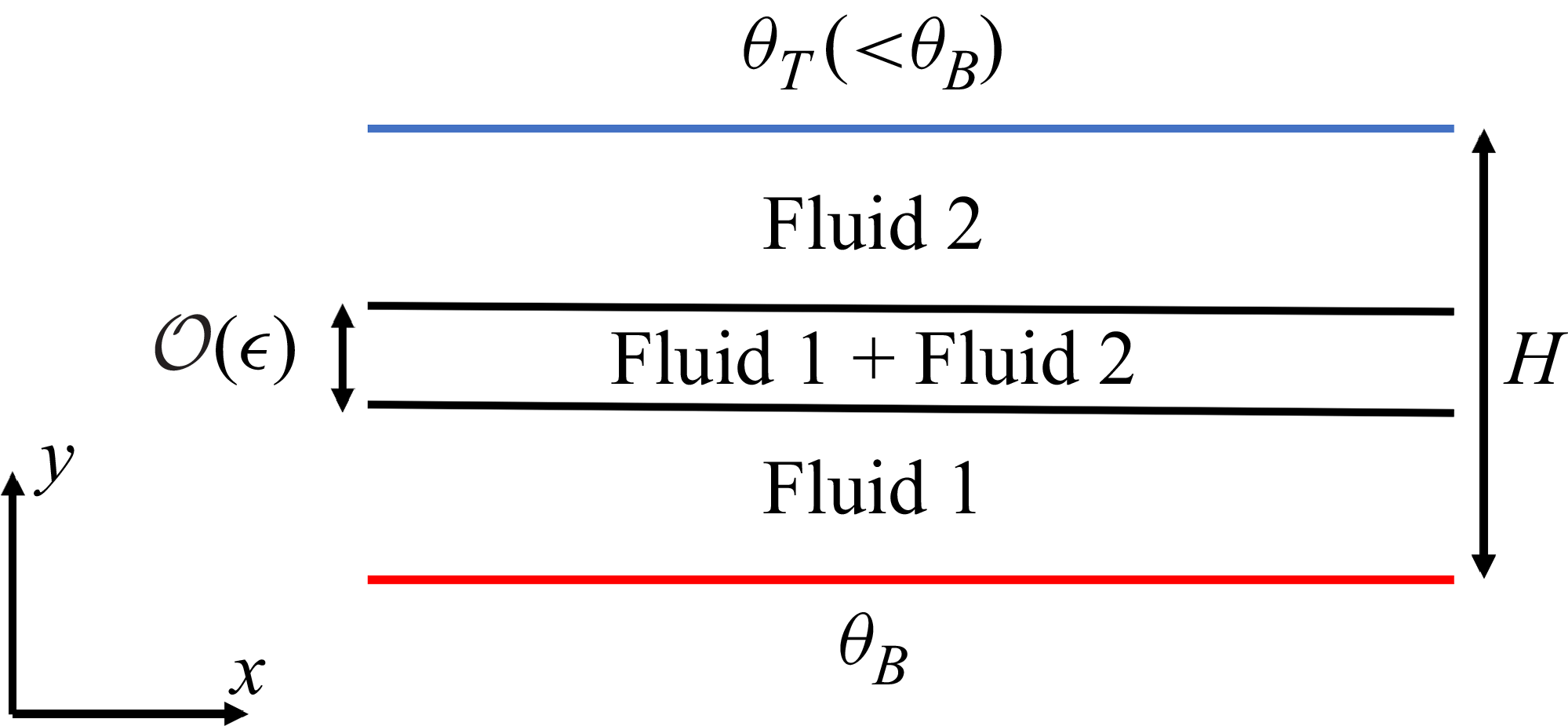
Schematic of RB convection problem in binary fluids. Here,
 $\theta_B$
and
 $\theta_T$
is the temperature of the bottom and top plates, respectively.
 $\epsilon$
represents the thickness of the diffuse-interface.

In this section, we define a suitable model for phase transition in binary fluids and subsequently describe the set of equations that governs the onset of RBM convection in such systems when they are slightly below the UCST. The configuration of the present system is shown in figure 1 wherein the lighter fluid is stacked over the heavier one, and the system is infinite in horizontal directions. The top and bottom walls are maintained at uniform temperatures, with the bottom being hotter than the top. The fluid interface is diffuse, and its thickness diverges as the system approaches the UCST. We mimic this interfacial behaviour through a phase-field model that utilises the fluid free energy to smoothen the interfacial effects over a thin, numerically resolvable region. The simplest form of this free-energy-density functional (Jacqmin Reference Jacqmin1999) can be written as
 \begin{align} f\left ( \phi ,\boldsymbol {\nabla }\phi \right ) = \mathcal{A}_1 \varPsi \left (\phi \right ) + \frac {1}{2}\mathcal{A}_2\left | \boldsymbol{\nabla }\phi \right |^2, \end{align}
where
 $\phi$
is the phase-field parameter that helps identify the bulk phases and the intervening interface;
 $\mathcal{A}_1$
and
 $\mathcal{A}_2$
are constants related to the surface tension coefficient and the thickness of the diffuse interface. The first term on the right-hand side of (2.1) represents the bulk energy part, which, for a two-phase/two-layer system, forms a double-well potential in the free energy versus phase-parameter diagram. Different forms of bulk energy expression are generally used to mimic this double-well behaviour. The form,
 $\varPsi (\phi ) = (\phi ^2 - 1)^2$
(Yue et al. Reference Yue, Feng, Liu and Shen2004; Celani et al. Reference Celani, Mazzino, Muratore-Ginanneschi and Vozella2009), is the most widely used, where
 $\phi _{bp}=\pm 1$
represent the bulk phases. Other varieties like
 $\varPsi (\phi ) = (\phi ^2 - 1/4)^2$
and
 $\varPsi (\phi ) = (\phi ^2 - 1/4)^{3/2}$
, where
 $\phi _{bp} = \pm 1/2$
, can also be used (Jacqmin Reference Jacqmin1999). The second term in (2.1) represents the gradient energy required for sustaining the interface between the two phases. This gradient part accounts for the weak non-local interaction between the components (Yue et al. Reference Yue, Feng, Liu and Shen2004) and is responsible for the formation of the mixing layer between the two fluids (Celani et al. Reference Celani, Mazzino, Muratore-Ginanneschi and Vozella2009). The competition between the philic (gradient energy) and the phobic (bulk mixing energy) effects (Yue et al. Reference Yue, Feng, Liu and Shen2004) determines the structure of the interface. Typically, the width of the interface is proportional to
 $\sqrt {\mathcal{A}_2/\mathcal{A}_1}$
and the surface tension is proportional to
 $\sqrt {\mathcal{A}_1\mathcal{A}_2}$
. In the case of miscibility transition in the binary fluids, the double-well potential transforms to a single-well as the system temperature transitions over the UCST. Bestehorn et al. (Reference Bestehorn, Sharma, Borcia and Amiroudine2021) proposed the following free-energy functional to capture this transition:
 \begin{align} f\left ( \phi , \boldsymbol {\nabla }\phi \right ) = \mathcal{A}_1 \big [ \mathcal{H}(r) r^q \phi ^4 - 2 r \phi ^2 \big ] + \frac {1}{2} \mathcal{H}\left (r\right ) \mathcal{A}_2 r^p \left | \boldsymbol{\nabla }\phi \right |^2, \end{align}
with
 $p$
and
 $q$
being the model constants. In the functional,
 $r$
(defined later) provides information on the base operating condition of the system, wherein
 $r=1$
indicates that the system is far below the upper consolute temperature of the fluids, and its value diminishes as the system approaches the UCST. When
 $r$
is negative, the system temperature will be above the UCST, and the components are completely miscible with no intervening interfaces. The Heaviside step function,
 $\mathcal{H}(r)$
, is zero for any negative
 $r$
and is one otherwise. Thus,
 $r$
, in combination with
 $\mathcal{H}(r)$
, provides a convenient means for modelling the immiscible-to-miscible phase transition. In other words, for any positive values of
 $r$
, the bulk part of the free energy manifests as a double-well potential in the phase diagram (figure 2), denoting the co-existence of two phases. Beyond the critical or transition temperature (
 $\theta _{crit}$
), i.e. when
 $r \lt 0$
, the manifestation turns into a single-well structure.
The bulk free energy versus phase-parameter diagram showing the transition from a double-well structure to a single-well one with a decrease in the value of
 $r$
.

Since the present RB convection system is non-isothermal, the free-energy expression in (2.2) needs to be modified in line with the formulation suggested by Alt & Pawlow (Reference Alt and Pawlow1992) and Antanovskii (Reference Antanovskii1995). Correspondingly, the free energy of this non-isothermal system is given as
 \begin{align} F\left (\phi , \theta , \boldsymbol{\nabla }\phi \right ) = \int _\varOmega \left [ f_{bulk}(\phi ,\theta ) + \mathcal{H}(r) \frac {\varLambda }{2} r^p \left | \boldsymbol{\nabla }\phi \right |^2 \right ] \mathrm{d\boldsymbol{x}}, \end{align}
where
 \begin{align} f_{bulk}(\phi ,\theta ) = \rho c(\phi )\theta - \rho c(\phi )\theta \log {\theta } + \mathcal{H}(r)\frac {\varLambda }{4\epsilon ^2} r^q \phi ^4 - \frac {\varLambda }{2\epsilon ^2} r \phi ^2. \end{align}
where
 $ c $
is the specific heat capacity of the mixture. Note that the first two terms in the bulk energy expression correspond to the changes in internal energy and entropy caused by changes in temperature. Equation (2.3) is similar to the classical Ginzburg–Landau free-energy expression wherein
 $\varLambda$
is the magnitude of the mixing free energy of the system (Celani et al. Reference Celani, Mazzino, Muratore-Ginanneschi and Vozella2009). Here, the internal energy part is considered to be a linear function of
 $\phi$
.
The miscibility transition parameter,
 $r$
, is defined as
 \begin{align} r = \frac {\exp {(-a\vartheta )}-\exp {(a\vartheta )}}{\exp {(-a\vartheta )}+(Le)\exp {(a\vartheta )}}, \end{align}
where the reduced temperature
 $\vartheta$
is defined as
 $(\theta -\theta _{crit})/\theta _{crit}$
,
 $a$
is a positive constant, and
 $Le$
is the Lewis number, which gives the ratio of thermal diffusivity to the mass diffusivity of the components involved.
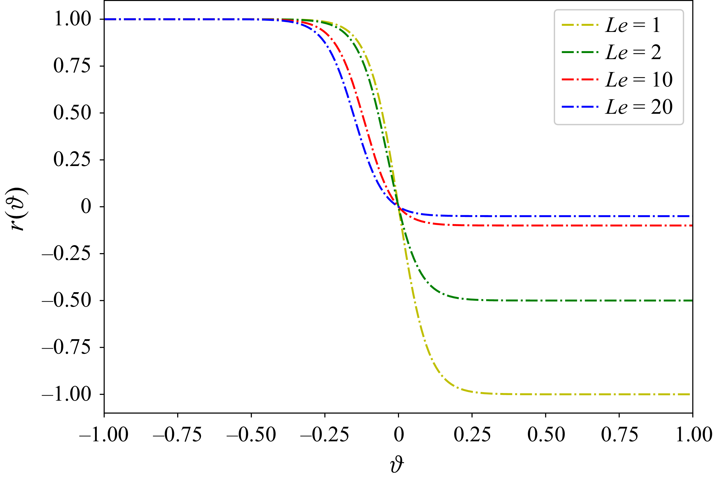
Variation of
 $r$
with
 $\vartheta$
for different values of
 $Le$
.

Figure 3 gives an idea of how
 $r$
varies with
 $\vartheta$
for
 $a=10$
and different values of
 $Le$
. It can be observed that
 $r$
is equal to one when the system is far below the UCST, and it saturates to a value of
 $-({1}/{Le})$
when the system is above the UCST. Typically,
 $r$
is spatially inhomogeneous in a non-isothermal domain. However, this inhomogeneity can be deemed insignificant in the present case of two-layer RBM convection, as we are only interested in the onset behaviour, which normally occurs within a critical temperature difference of the order of 1 K (Degen et al. Reference Degen, Colovas and Andereck1998). From figure 3, it is evident that
 $r$
reduces from a value of one to
 $-({1}/{Le})$
in the range of
 $\vartheta$
between
 $-0.375$
and
 $0.125$
. In reality, this
 $\vartheta$
range corresponds to a large change in the absolute temperature for a binary fluid system like FC-72 and 1cSt Silicone Oil with UCST = 315.5 K (Jajoo Reference Jajoo2017; Diwakar et al. Reference Diwakar, Jajoo, Amiroudine, Matsumoto, Narayanan and Zoueshtiagh2018). Thus, the rate of change of
 $r$
with temperature is meagre. This also implies that any fluctuations in
 $r$
would be orders of magnitude lower than the temperature fluctuations. It may be worth noting that the inhomogeneity in base
 $r$
, which is proportional to the base temperature gradient, can be easily subdued by considering thicker fluid layers that will result in smaller
 $\Delta T_{\textit{critical}}$
for the onset of buoyancy-driven convection. Hence, we consider a spatially homogeneous
 $r$
in the present work, as it also helps make the complex problem at hand more tractable.
With these considerations, we now formulate the governing equations for the evolution of RBM convection in the binary fluid system. Here, the phase parameter is evolved using a scalar transport equation wherein the diffusion process is driven by the gradients of chemical potential (Anderson et al. Reference Anderson, McFadden and Wheeler1998),
 $\mu$
, given as
 \begin{align} \mu = \frac {\delta F}{\delta \phi } = \varLambda \left [\frac {\mathcal{H}(r) r^q \phi ^3 - r \phi }{\epsilon ^2} - \mathcal{H}(r)r^p {\nabla} ^2\phi \right ]\!. \end{align}
We have assumed
 $\rho _1 c_1 \approx \rho _2 c_2$
to simplify our calculations. Note that
 $\rho _1$
and
 $\rho _2$
are the individual (unmixed) densities of the fluids 1 and 2, respectively, and
 $c_1$
and
 $c_2$
are the specific heat capacities of fluids 1 and 2, respectively. We focus mainly on the purely immiscible to partially miscible range where the value of
 $r$
is positive, i.e.
 $0.005\leqslant r \leqslant 1.0$
. This implies that
 $\mathcal{H}(r) = 1$
for all further considerations. The effect of diffuse interface on the fluid momentum is modelled here via the forcing term,
 $\boldsymbol {\nabla }\boldsymbol{\cdot }\boldsymbol{\tau }^{nv}$
, where
 $\boldsymbol{\tau}^{nv}$
is the non-viscous (reversible) stress tensor. The energy equation accounts for internal energy changes arising from both thermal transport and fluid mixing. Correspondingly, the coupled set of equations governing the phase evolution and mass, momentum and energy conservation is given as
 \begin{align} \frac {\partial \phi }{\partial t} + \boldsymbol{u}\boldsymbol{\cdot }\boldsymbol{\nabla }\phi = \boldsymbol{\nabla }\boldsymbol{\cdot } \left [\gamma \boldsymbol{\nabla }\bigg\{\varLambda \left (\frac {r^q \phi ^3 - r \phi }{\epsilon ^2} - r^p {\nabla} ^2\phi \right )\bigg \}\right], \\[-25pt] \nonumber \end{align}
 \begin{align} \frac {\partial \rho ^* \boldsymbol{u}}{\partial t} + \boldsymbol {\nabla }\boldsymbol{\cdot }(\rho ^*\boldsymbol{u}\boldsymbol{u}) = - \boldsymbol{\nabla }p + {\boldsymbol{\nabla }} \boldsymbol{\cdot } \! \left (\eta ^* \! \left ( \boldsymbol{\nabla }\boldsymbol{u} + (\boldsymbol{\nabla }\boldsymbol{u})^{+} - \dfrac {2}{3} \boldsymbol{\nabla }\boldsymbol{\cdot }\boldsymbol{u} \boldsymbol{I}\right )\right ) + \boldsymbol{\nabla }\boldsymbol{\cdot } \boldsymbol{\tau }^{nv} - \rho ^{\prime } g \boldsymbol{1}_y, \\[-30pt] \nonumber \end{align}
 \begin{align} \frac {{\rm D}\rho ^*}{{\rm D}t} + \rho ^* \boldsymbol{\nabla }\boldsymbol{\cdot } \boldsymbol{u} = 0, \\[-25pt] \nonumber \end{align}
 \begin{align} \frac {\partial \rho ^*(c^*\theta )}{\partial t} + \boldsymbol {\nabla }\boldsymbol{\cdot }(\rho ^*\boldsymbol{u} c^*\theta ) + \varLambda _0\left [\frac {r^q \phi ^3 - r \phi }{\epsilon ^2} - r^p {\nabla} ^2\phi \right ] \frac {{\rm D}\phi }{{\rm D}t} + \mathcal{L}\boldsymbol{\nabla }\boldsymbol{\cdot }\boldsymbol{u} = \boldsymbol{\nabla }\boldsymbol{\cdot } (\kappa ^* \boldsymbol{\nabla }\theta ), \end{align}
where
 \begin{align} \boldsymbol{\tau }^{nv} = \mathcal{L} \boldsymbol{I} - \boldsymbol{\nabla }\phi \frac {\partial \mathcal{L}}{\partial (\boldsymbol{\nabla }\phi )} \end{align}
and
 $\mathcal{L} = f_{bulk}(\phi ,\theta ) + \mathcal{H}(r) ( {\varLambda }/{2}) r^p | \boldsymbol{\nabla }\phi (x)|^2$
is the Lagrangian energy density. Here,
 $\rho ^*$
,
 $c^*$
and
 $\eta ^*$
are the mixture density, heat capacity and dynamic viscosity, respectively, and
 $\rho ^{\prime }$
in (2.8) corresponds to
 $\rho ^* - {\rho }_{0}$
, where
 ${\rho }_{0}$
is the base density at any location and is given as
 $\rho _0(\phi ) = \rho _1( ({1+\phi })/{2}) + \rho _2(({1-\phi })/{2})$
. The present formulation precludes the direct implementation of the classical Boussinesq approximation, which assumes homogeneity of density everywhere, except in the buoyancy term that drives the convection (Spiegel & Veronis Reference Spiegel and Veronis1960; Drazin & Reid Reference Drazin and Reid2004). Such an approximation would have been admissible only in fluid systems with very small density disparity. Since we do not impose such restrictions on the fluids, we proceed with the inhomogeneous base density formulation, which results in
 $\rho ^*$
being set as
 ${\rho }_{0}$
in the left-hand side of (2.8), (2.9) and (2.10).
Incidentally, the current configuration of the system falls under the class of quasi-incompressible fluids, wherein the velocity field in the mixing region is non-solenoidal despite the bulk fluids being incompressible. This results in the chemical potential becoming a function of pressure. Since the pressure is determined here from kinematics and not from thermodynamics, the overall mathematical formulation and its analysis become complicated. It can be shown that the issue of non-solenoidal velocity in the mixing region arises from the way the velocity field has been formulated in the multi-phase domain. In the following subsection, we look at an alternative means of defining the velocity field such that it becomes solenoidal everywhere.
2.1. Volume-averaged velocity field
The velocity field often considered in general one-fluid frameworks is inherently a mass-averaged/barycentric quantity (Joseph et al. Reference Joseph, Huang and Hu1996) given as
 \begin{align} \boldsymbol{u} = \frac {\tilde {\rho }_1\boldsymbol{u}_1 + \tilde {\rho }_2\boldsymbol{u}_2}{\rho _0}, \end{align}
where
 $\tilde {\rho }_1$
and
 $\tilde {\rho }_2$
are the apparent densities of the fluids 1 and 2, defined as
 $\tilde {\rho }_1 = \rho _1(({1+\phi })/{2})$
and
 $\tilde {\rho }_2 = \rho _2(({1-\phi })/{2})$
,
 $\boldsymbol{u}_1$
and
 $\boldsymbol{u}_2$
are the velocities of fluids 1 and 2, respectively. This mass-averaged velocity satisfies the classical continuity equation
 $\partial _t \rho _0 + {\boldsymbol{\nabla }}\boldsymbol{\cdot }(\rho _0\boldsymbol{u}) = 0$
. However, it results in a non-solenoidal velocity field, primarily in the diffuse interfacial region. In order to overcome this issue, we will now redefine the velocity field as a volume-averaged quantity (Boyer Reference Boyer2002; Ding et al. Reference Ding, Spelt and Shu2007; Abels et al. Reference Abels, Garcke and Grun2012) such that it becomes solenoidal throughout the system, including the interfacial region. Correspondingly, we use
 \begin{align} \boldsymbol{u} = \frac {\tilde {\rho }_1}{\rho _1} \boldsymbol{u}_1 + \frac {\tilde {\rho }_2}{\rho _2} \boldsymbol{u}_2. \end{align}
Using the mass conservation equations of the individual species, i.e.
 $\partial _t \tilde {\rho }_j + {\boldsymbol {\nabla }}\boldsymbol{\cdot }(\tilde {\rho }_j\boldsymbol{u}_j) = 0$
, one can show (2.13) to yield a solenoidal velocity field throughout the domain:
 \begin{align} {\boldsymbol {\nabla }}\boldsymbol{\cdot }\boldsymbol{u} &= {\boldsymbol{\nabla }}\boldsymbol{\cdot }\left ( \frac {\tilde {\rho }_1 \boldsymbol{u}_1}{\rho _1} \right ) + {\boldsymbol{\nabla }}\boldsymbol{\cdot }\left ( \frac {\tilde {\rho }_2 \boldsymbol{u}_2}{\rho _2} \right )\nonumber \\ &= - \partial _t \left ( \frac {\tilde {\rho }_1}{\rho _1} \right ) - \partial _t \left ( \frac {\tilde {\rho }_2}{\rho _2} \right )\nonumber \\ &= - \partial _t \left ( \frac {\tilde {\rho }_1}{\rho _1} + \frac {\tilde {\rho }_2}{\rho _2} \right )\nonumber \\ &= -\partial _t (1) = 0.\end{align}
Consequently, the overall mass balance equation gets modified as (Ding et al. Reference Ding, Spelt and Shu2007)
 \begin{align} \partial _t \rho _0 + {\boldsymbol {\nabla }}\boldsymbol{\cdot }(\rho _0\boldsymbol{u}) - \frac {\partial \rho _0}{\partial \phi }{\boldsymbol{\nabla }} \boldsymbol{\cdot }\left (\gamma \boldsymbol{\nabla }\mu \right ) = 0. \end{align}
2.2. Governing equations and boundary conditions
Following this modification in the velocity-averaging process, the equations governing RBM convection in binary fluid systems can be simplified by rewriting them in the non-conservation form. To account for the Marangoni effect, the magnitude of mixing free energy is considered as a linear function of temperature. Since the temperature fluctuations are expected to be small at onset, one can use the Taylor series expansion to write the free-energy magnitude as
 $\varLambda = \varLambda _0 + (\partial \varLambda / \partial \theta ) \theta$
. Correspondingly, the full set of governing equations is written as
 \begin{align} \frac {\partial \phi }{\partial t} + \boldsymbol{u} \boldsymbol{\cdot }\boldsymbol{\nabla }\phi = \boldsymbol{\nabla }\boldsymbol{\cdot }\left [\gamma { \boldsymbol{\nabla }} \bigg \{{\varLambda }\left (\frac {r^q \phi ^3 - r \phi }{\epsilon ^2} - r^p {\nabla} ^2\phi \right )\bigg\} \right ]\!, \\[-25pt] \nonumber \end{align}
 \begin{align} \boldsymbol {\nabla }\boldsymbol{\cdot } \boldsymbol{u} = 0, \\[-28pt] \nonumber \end{align}
 \begin{eqnarray} \nonumber \rho _0 \left ( \frac {\partial \boldsymbol{u}}{\partial t} + \boldsymbol{u}\boldsymbol{\cdot }{\boldsymbol {\nabla }}\boldsymbol{u} \right ) = & - {\boldsymbol{\nabla }} p + {\boldsymbol{\nabla }} \boldsymbol{\cdot }\big (\eta ^* \left ( {\boldsymbol{\nabla }}\boldsymbol{u} + ({\boldsymbol{\nabla }}\boldsymbol{u})^{+}\right )\big ) - \rho ^{\prime } g \hat {\boldsymbol{1}}_y \qquad \qquad \quad \\&- r^p \varLambda {\nabla} ^2\phi \boldsymbol{\nabla }\phi + \frac {1}{3} r^p \left | \boldsymbol{\nabla }\phi \right |^2 \frac {\partial \varLambda }{\partial \theta } {\boldsymbol{\nabla }}\theta \nonumber \\ &- \frac {1}{6} \varLambda r^p \boldsymbol{\nabla }\left |\boldsymbol{\nabla }\phi \right |^2 - r^p {\boldsymbol{\nabla }}\phi \frac {\partial \varLambda }{\partial \theta } {\boldsymbol{\nabla }}\theta \boldsymbol{\cdot }{\boldsymbol{\nabla }}\phi , \\[-25pt] \nonumber \end{eqnarray}
 \begin{align} \rho _0 c^* \bigg (\frac {\partial \theta }{\partial t} + \boldsymbol{u}\boldsymbol{\cdot }{ \boldsymbol{\nabla }}\theta \bigg ) + \varLambda _0\left [\frac {r^q \phi ^3 - r \phi }{\epsilon ^2} - r^p {\nabla} ^2\phi \right ] \frac {{\rm D}\phi }{{\rm D}t} = {\boldsymbol{\nabla }} \boldsymbol{\cdot }(\kappa ^* \boldsymbol{\nabla }\theta ), \\[0pt] \nonumber \end{align}
where
 $\rho ^{\prime } = \rho ^*(\phi ,\theta ) - \rho _0$
and
 $\rho ^*(\phi ,\theta ) = \rho _1( 1-\beta _1(\theta -\theta _0) )( ({1+\phi })/{2}) + \rho _2( 1-\beta _2 (\theta -\theta _0) )(({1-\phi })/{2})$
,
 $\beta_1$
and
 $\beta_2$
are the unmixed thermal expansivities of the fluids 1 and 2, respectively. In (2.18), the isotropic contributions to the reversible stress (2.11) have been absorbed into the pressure term. Only the anisotropic part that contributes towards the dynamics (Cates & Tjhung Reference Cates and Tjhung2018) has been written explicitly. The detailed derivations of this set of equations and their subsequent linearisation have been presented in the supplementary material available at https://doi.org/10.1017/jfm.2026.11206.
At the top and bottom (figure 1), no-slip walls are considered with constant temperatures. Correspondingly, we write the boundary conditions as
 \begin{align} \boldsymbol{u} &= 0 \,\,\,@ y = 0, H,\end{align}
 \begin{align} \theta & = \theta _B \,\,\,@ y = 0,\end{align}
 \begin{align} \theta &= \theta _T \,\,\,@ y = H,\end{align}
where
 $ H $
is the total height of the system. Note that the phase evolution equation obeys the no-flux boundary condition owing to the consideration of impermeable no-slip walls at the top and bottom. Thus, we have
 \begin{align} \boldsymbol{1}_y \boldsymbol{\cdot } \boldsymbol{\nabla }\phi = 0 \,\,\,@ y = 0, H,\end{align}
 \begin{align} \boldsymbol{1}_y \boldsymbol{\cdot } \boldsymbol{\nabla }\mu = 0 \,\,\,@ y = 0, H.\end{align}
Since,
 $\mu = \varLambda [( ({r^q \phi ^3 - r \phi })/{\epsilon ^2}) - r^p {\nabla} ^2\phi ]$
, we simplify these conditions as
 \begin{align} \frac {\partial \phi }{\partial y} = \frac {\partial ^3\phi }{\partial y^3} = 0 \,\,\,@ y = 0, H .\end{align}
Here,
 $\varLambda$
has been treated as a weak function of temperature at the walls, which are constant values. Finally, the various properties of the fluid mixture can be expressed as a linear function of
 $\phi$
as follows:
-
(i) density,
 ${\rho _0}/{\rho _2} = ( {1}/{2}) (1+\rho ) + ({\phi }/{2}) ( \rho -1 )$
;
-
(ii) dynamic viscosity,
$ {\eta ^*}/{\eta _2} = ( {1}/{2})( 1+\eta ) + ({\phi }/{2}) ( \eta -1 )$
; -
(iii) thermal conductivity,
${\kappa ^*}/{\kappa _2} = ( {1}/{2}) ( 1+\kappa ) + ({\phi }/{2}) ( \kappa -1 )$
; -
(iv) heat capacity,
${\rho _0 c^*}/({\rho _2 c_2}) = ( {1}/{2}) (1+ \rho c ) + ({\phi }/{2}) ( \rho c - 1 )$
; and -
(v) thermal expansion coefficient,
${\rho _0 \beta ^*}/({\rho _2 \beta _2}) = ( {1}/{2}) (1+ \rho \beta ) + ({\phi }/{2}) ( \rho \beta - 1 )$
.


Here,
 $\rho \;(={\rho _1}/{\rho _2})$
is the density ratio,
 $\eta \;(={\eta _1}/{\eta _2})$
is the dynamic viscosity ratio,
 $\beta \;(={\beta _1}/{\beta _2})$
is the ratio of thermal expansion coefficients,
 $\kappa \;(={\kappa _1}/{\kappa _2})$
is the thermal conductivity ratio, and
 $c\;(={c_1}/{c_2})$
is specific heat ratio. While these ratios correspond to the properties of the pure fluids, we also define a few apparent property ratios such as
 $\tilde {\rho }$
,
 $\tilde {\beta }$
, and
 $\tilde {\alpha }$
that correspond to the properties of the fluid layers that vary with the miscibility parameter. In fact, each of these ratios approaches unity as the system gets closer to the critical point.
3. Linear stability analysis
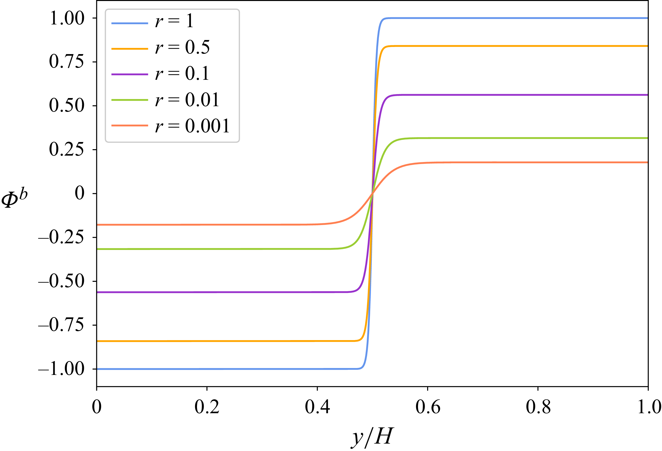
Phase distribution in the system for different
 $r$
.

Using the diffuse-interface formulation, we now analyse the onset characteristics of RBM convection in binary fluids closer to their UCST. To this effect, we perform a linear stability analysis to evaluate the critical parameters and the associated modes of convection, which could be either oscillatory or non-oscillatory. Note that the oscillatory modes of onset are observed in a purely immiscible RB scenario when the MC and TC modes compete with each other. This situation of overstability typically occurs when the value of
 $\rho \beta \alpha$
differs significantly from unity (Renardy Reference Renardy1996). The present goal is to understand how such oscillatory modes transform for a diffuse interface, particularly when its thickness diverges near the critical point.
The present base state consists of two quiescent layers of fluids with imposed uniform temperatures at the top and bottom walls. Note that the bottom wall’s temperature is higher than that of the top and, at the same time, does not exceed the UCST of the mixture. As mentioned earlier, the miscibility transition parameter,
 $r$
, is assumed to be uninfluenced by the imposed spatial inhomogeneity in temperature. We accordingly consider a homogeneous
 $r$
in the domain that corresponds to the interfacial temperature. In fact,
 $r$
is used here to define the state of the system, and we consider different
 $r$
values ranging from 0.005 to 1, representing the system’s closeness (or otherwise) to the UCST. Thus, for a given value of
 $r$
, the base profile of the order parameter (
 $\varPhi ^b$
) can be obtained by considering a trivial chemical potential, i.e.
 $\mu = 0$
. The resulting expression for
 $\varPhi ^b$
can be written as
 \begin{align} \varPhi ^b(y) = \pm r^{tfrac {1-q}{2}} \tanh \left (\frac {y}{\sqrt {2}\epsilon } r^{tfrac {1-p}{2}} \right )\!. \end{align}
Figure 4 shows the variation of
 $\varPhi ^b$
with decreasing
 $r$
, i.e. with increasing operating temperature. It is evident that the peak value of
 $\varPhi^b$
reduces in both the layers owing to the enhanced solubility of the phases. The interfacial width, being proportional to
 $r^{({p-1})/{2}}$
, increases with the increase in system temperature. Here, the contribution of the gradient energy term decreases, and more material is introduced into the interfacial region, thereby creating a wider interface.
Along with (3.1), the quiescent base state is represented here through the following expressions for pressure and temperature distribution:
 \begin{align} \boldsymbol {\nabla }p^b(y) & + r^p \varLambda (\varTheta ^b) {\nabla} ^2\varPhi ^b \boldsymbol{\nabla }\varPhi ^b - \frac {1}{3} r^p \big |\boldsymbol{\nabla }\varPhi ^b\big |^2 \frac {\partial \varLambda }{\partial \theta } {\boldsymbol{\nabla }}\varTheta ^b \nonumber \\& + \frac {1}{6} \varLambda (\varTheta ^b) r^p \boldsymbol{\nabla }\big |\boldsymbol{\nabla }\varPhi ^b\big |^2 + r^p {\boldsymbol{\nabla }}\varPhi ^b \frac {\partial \varLambda }{\partial \theta } {\boldsymbol{\nabla }}\varTheta ^b\boldsymbol{\cdot }{ \boldsymbol{\nabla }}\varPhi ^b = - \rho ^{\prime } \big (\varPhi ^b, \varTheta ^b\big )g \boldsymbol{1}_y, \\[-28pt] \nonumber \end{align}
 \begin{align} \boldsymbol {\nabla }\boldsymbol{\cdot }\big (\kappa (\varPhi ^b) \boldsymbol{\nabla }\varTheta ^b(y)\big ) = 0, \\[-28pt] \nonumber \end{align}
 \begin{align} L_R = H, \quad t_R = \frac {{H}^2}{\alpha _2}, \quad u_R = \frac {\alpha _2}{H}, \quad \theta _R = \theta _B - \theta _T, \quad p_R = \frac {\rho _2 \alpha _2 \nu _2}{{H}^2}. \\[0pt] \nonumber \end{align}
where
 $\Theta^{b}$
is the base-state (no-flow) temperature profile and
 $\alpha_2$
and
 $\nu_2$
are the thermal diffusivity and the kinematic viscosity of fluid 2, respectively. The non-dimensionalisation of all the variables has been performed in the current formulation using the scales that correspond to the top layer. Correspondingly, we arrive at four relevant dimensionless numbers: (i) the non-dimensional mobility,
 $M\;(= \gamma \varLambda _0/(\epsilon ^2\alpha _2))$
, which is the ratio of the interfacial diffusivity to the thermal diffusivity of the reference fluid, (ii) the modified inverse capillary number,
 $\varGamma _\theta \;(= \varLambda _0/(\rho _2 \alpha _2^2))$
, where the word `modified’ refers to the non-standard usage of thermal diffusivity instead of the kinematic viscosity, (iii) the inverse capillary number,
 $Ca \;(= \sigma _0 H/(\eta_2 \alpha _2))$
where
 $\sigma_0$
is the coefficient of surface tension in absence of temperature inhomogeneity.
 $\eta_2$
is the dynamic viscosity of fluid 2 and (iv) the Marangoni number,
 $Ma\;(=\sigma _\theta \Delta \theta H/(\eta _2\alpha _2))$
where
 $\sigma_{\theta}$
is the magnitude of the surface-tension gradient with respect to temperature. Since the Marangoni
 $(Ma)$
and the Rayleigh numbers,
 $Ra\;(= g \rho _2 \beta _2 \Delta \theta H^3/(\eta _2\alpha _2))$
, are not independent, an additional non-dimensional parameter,
 $\zeta$
, has been defined (as follows) to link the two. Here, we have considered
 $\sigma =\sigma _0 - \sigma _\theta \theta$
:
 \begin{align} \zeta = \frac {Ma}{Ra} = \frac {\sigma _\theta }{g\rho _2\beta _2 H^2} . \\[-10pt] \nonumber \end{align}
Linearising the governing equations ((2.16) to (2.19)) and the boundary conditions over the base state, we obtain the ensuing set of equations that govern the evolution of perturbations in the domain:
 \begin{align} \frac {\partial \phi ^{\prime }}{\partial t} + {u}_j^{\prime }{\nabla}_j\varPhi ^b = M {\nabla} ^2 \left [ \left (1 - \frac {\zeta Ra}{Ca} \varTheta ^{b}\right ) \left ( r^q 3(\varPhi ^b)^2\phi ^{\prime } - r \phi ^{\prime } - \left ( \frac {\epsilon }{H} \right )^2 r^p {\nabla} ^2\phi ^{\prime } \right ) \right ], \\[-28pt] \nonumber \end{align}
 \begin{align} {\rho _f^b}\frac {\partial {u}_i^{\prime }}{\partial t} = &- Pr_2 {\nabla}_i p^{\prime } + Pr_2 {\nabla}_j \left [ \left ( \frac {1}{2}(1+\eta ) + \frac {\varPhi ^b}{2}(\eta -1) \right ) \big ( {\nabla}_j u_i^{\prime } + {\nabla}_i u_j^{\prime } \big ) \right ] \nonumber \\&+ Ra Pr_2 \frac {1}{2}\left (\rho \beta -1\right ) \varTheta ^b \phi ^{\prime } \delta _{i2} + Ra Pr_2 \left [\frac {1}{2}\left (\rho \beta +1\right ) + \frac {1}{2}\left (\rho \beta -1\right ) \varPhi ^{b} \right ] \theta ^{\prime } \delta _{i2} \nonumber \\&+ \left (\frac {H}{\epsilon }\right )^2 \varGamma _\theta \left ( r^q 3(\varPhi ^b)^2 \phi ^{\prime } - r \phi ^{\prime } - \left (\frac {\epsilon }{H}\right ) ^2 r^p {\nabla} ^2 \phi ^{\prime } \right ){\nabla}_{i}\varPhi ^{b} \nonumber \\&- \frac {3}{2\sqrt {2}} \zeta Ra Pr_2 \frac {H}{\epsilon } \left [\varTheta ^b \left ( r^q 3(\varPhi ^b)^2 \phi ^{\prime } - r \phi ^{\prime } - \left (\frac {\epsilon }{H}\right ) ^2 r^p {\nabla} ^2 \phi ^{\prime } \right ){\nabla}_{i}\varPhi ^{b} \right ] \nonumber \\&- \frac {3}{2\sqrt {2}} \zeta Ra Pr_2 \frac {\epsilon }{H} r^p {\nabla}_{i}\varTheta ^b {\nabla} ^2\varPhi ^b \phi ^{\prime } \nonumber \\&+ \frac {3}{2\sqrt {2}} \zeta Ra Pr_2 \frac {\epsilon }{H} r^p \frac {1}{3} \left [\varTheta ^b \big (\partial _y\varPhi ^b {\nabla}_{i}(\partial _y\phi ^{\prime }) + {\nabla}_{i}(\partial _y\varPhi ^b) \partial _y\phi ^{\prime }\big ) \right ] \nonumber \\&+ \frac {3}{2\sqrt {2}} \zeta Ra Pr_2 \frac {\epsilon }{H} r^p \frac {1}{3} \partial _y\varPhi ^b {\nabla}_{i}\big (\partial _y\varPhi ^b\big ) \theta ^{\prime } \nonumber \\&+ \frac {3}{2\sqrt {2}} \zeta Ra Pr_2 \frac {\epsilon }{H} r^p {\nabla} ^2\varPhi ^b{\nabla}_{i}\varPhi ^b\theta ^{\prime } \nonumber \\&- \frac {3}{2\sqrt {2}} \zeta Ra Pr_2 \frac {\epsilon }{H} r^p \left ( \frac {1}{3} \left |{\nabla} _k\varPhi ^b\right |^2 {\nabla}_{i}\theta ^{\prime } + \frac {2}{3} {\nabla} _k\varPhi ^b {\nabla} _k\phi ^{\prime } {\nabla}_{i}\varTheta ^b\right )\nonumber\\& +\! \frac {3}{2\sqrt {2}} \zeta Ra Pr_2 \frac {\epsilon }{H} r^p \big ({\nabla}_{i}\varPhi ^b \big ({\nabla}_{\kern-2pt j}\varTheta ^b {\nabla}_{\kern-2pt j}\phi ^{\prime } \!+\! {\nabla}_{\kern-2pt j}\theta ^{\prime } {\nabla}_{\kern-2pt j}\varPhi ^b \big ) \!+\! {\nabla}_{i}\phi ^{\prime } {\nabla}_{\kern-2pt j}\varTheta ^b {\nabla}_{\kern-2pt j}\varPhi ^b \big ) , \\[-45pt] \nonumber \end{align}
 \begin{eqnarray} &&\nonumber \\ &&{\nabla}_j {u}_j^{\prime } = 0, \\[-28pt] \nonumber \end{eqnarray}
 \begin{eqnarray} (\rho c)_f^b\left [\frac {\partial \theta ^{\prime }}{\partial t} + {u_j}^{\prime } \frac {\partial \varTheta ^{b}}{\partial x_j} \right ] & = & \kappa _f(\varPhi ^b){\nabla _m}^2\theta ^{\prime } + ({\nabla} _m \kappa _f(\varPhi ^b))({\nabla} _m \theta ^{\prime }) \nonumber \\ &&+ ({\nabla} _m \kappa _f(\phi ^{\prime })) ({\nabla} _m \varTheta ^b) + \kappa _f(\phi ^{\prime }){{\nabla} _m}^2\varTheta ^{b}. \\[0pt] \nonumber \end{eqnarray}
 $Pr_2$
is the Prandtl number based on properties of fluid 2.
 $\delta_{i2}$
is the Kronecker-delta. In these equations, the property ratios,
 $(\rho c)_f^b$
and
 $\rho _f^b$
, are defined as
 \begin{align} (\rho c)_f^b & = \frac {1}{2} \left(1+\frac {\rho _1 c _1}{\rho _2 c _2} \right) + \frac {\varPhi ^b}{2} \left(\frac {\rho _1 c _1}{\rho _2 c _2}-1 \right),\end{align}
 \begin{align} \rho _f^b & = \frac {1}{2}(1+\rho ) + \frac {\varPhi ^b}{2}(\rho -1). \end{align}
For the current system configuration of infinite horizontal extents, the normal mode expansion of the perturbed quantities can be written as
 \begin{align} \left \{\phi ^{\prime }, \boldsymbol{u}^{\prime }, \theta ^{\prime }, p^{\prime }\right \}\left (x,y,t\right ) = \left \{\hat {\phi }(y), \hat {\boldsymbol{u}}(y), \hat {\theta }(y), \hat {p}(y)\right \}\exp {(\lambda t + \mathrm{i}kx)}, \end{align}
where
 $\lambda$
is the growth factor whose real part gives the growth rate of the perturbation and the imaginary part is associated with the speed of the traveling wave,
 $k^2 = k_1^2+k_2^2$
and
 $k_1$
,
 $k_2$
are the wavenumbers of the imposed disturbances along the two orthogonal horizontal directions. Here,
 $\hat {\boldsymbol{u}} = (\hat {u}, \hat {v} )$
, and
 $\hat {u} = ({k_1\hat {u}_1 + k_2\hat {u}_2})/{k}$
, with
 $\hat {u}_1$
and
 $\hat {u}_2$
being the amplitudes of the horizontal velocity components. Correspondingly, all the linearised perturbation equations get transformed as follows:
 \begin{align} \lambda \hat {\phi } & + \hat {v} \frac {\mathrm{d} \varPhi ^{b}}{\mathrm{d} y}\nonumber\\& = M \!\left [ 3 r^q \!\left ( -(\varPhi ^b)^2 k^2 \hat {\phi } + 2 \!\left(\frac {\mathrm{d}\varPhi ^{b}}{\mathrm{d}y} \right)^2 \hat {\phi } + 2 \varPhi ^b \frac {{\rm d}^2\varPhi ^b}{\mathrm{d}y^2} \hat {\phi } + 4\varPhi ^b \frac {\mathrm{d}\varPhi ^b}{\mathrm{d}y} \frac {\mathrm{d}\hat {\phi }}{\mathrm{d}y} + (\varPhi ^b)^2 \frac {{\rm d}^2\hat {\phi }}{\mathrm{d}y^2} \right ) \right . \nonumber \\ &\left . - r \left ( -k^2 \hat {\phi } + \frac {{\rm d}^2\hat {\phi }}{\mathrm{d}y^2} \right ) - \left (\frac {\epsilon }{H}\right ) ^2 r^p \left ( \frac {{\rm d}^4\hat {\phi }}{\mathrm{d}y^4} - 2 k^2 \frac {{\rm d}^2\hat {\phi }}{\mathrm{d}y^2} + k^4 \hat {\phi }\right ) \right ] \nonumber \\ &- M \left ( \frac {\zeta Ra}{Ca} \right ) \varTheta ^b \left [ 3 r^q ( -(\varPhi ^b)^2 k^2 \hat {\phi } + 2 \left (\frac {\mathrm{d}\varPhi ^{b}}{\mathrm{d}y}\right )^2 \hat {\phi } + 2 \varPhi ^b \frac {{\rm d}^2\varPhi ^b}{\mathrm{d}y^2} \hat {\phi } + 4\varPhi ^b \frac {\mathrm{d}\varPhi ^b}{\mathrm{d}y} \frac {\mathrm{d}\hat {\phi }}{\mathrm{d}y} \right . \nonumber \\ &\left . + (\varPhi ^b)^2 \frac {{\rm d}^2\hat {\phi }}{\mathrm{d}y^2} ) - r \left ( -k^2 \hat {\phi } + \frac {{\rm d}^2\hat {\phi }}{{\rm d}y^2} \right ) - \left (\frac {\epsilon }{H}\right ) ^2 r^p \left ( \frac {{\rm d}^4\hat {\phi }}{\mathrm{d}y^4} - 2 k^2 \frac {{\rm d}^2\hat {\phi }}{\mathrm{d}y^2} + k^4 \hat {\phi }\right ) \right ] \nonumber \\ &- 2 M \left ( \frac {\zeta Ra}{Ca} \right ) \frac {\mathrm{d}\varTheta ^b}{\mathrm{d}y} \left [ 3 r^q(\varPhi ^b)^2 \frac {\mathrm{d}\hat {\phi }}{\mathrm{d}y} + 6 r^q(\varPhi ^b) \frac {\mathrm{d}\varPhi ^b}{\mathrm{d}y} \hat {\phi } - r \frac {\mathrm{d}\hat {\phi }}{\mathrm{d}y}\right.\nonumber\\ & \left. - \left ( \frac {\epsilon }{H} \right )^2 r^p \left ( \frac {{\rm d}^2}{\mathrm{d}y^2} - k^2 \right ) \frac {\mathrm{d}\hat {\phi }}{\mathrm{d}y} \right ] \nonumber \\ &- M \left ( \frac {\zeta Ra}{Ca} \right ) \frac {{\rm d}^2\varTheta ^b}{{{\rm d}}y^2} \left ( r^q 3(\varPhi ^b)^2 \hat {\phi } - r \hat {\phi } - \left ( \frac {\epsilon }{H} \right )^2 r^p {\nabla} ^2\hat {\phi } \right )\!, \\[-28pt] \nonumber \end{align}
 \begin{align} {\rho _f(\varPhi ^b)} \lambda \hat {u} = &- Pr_2 (\mathrm{i} k) \hat {p} + Pr_2 \left [ \frac {1}{2}(1+\eta ) + \frac {\varPhi ^b}{2}(\eta -1) \right ] \left (-k^2+\frac {{\rm d}^2}{\mathrm{d}y^2}\right )\hat {u} \nonumber \\ & + Pr_2 \frac {1}{2}(\eta -1) \frac {\mathrm{d}\varPhi ^b}{\mathrm{d}y}\frac {\mathrm{d}\hat {u}}{\mathrm{d}y} + Pr_2 \frac {1}{2}(\eta -1) \frac {\mathrm{d}\varPhi ^b}{\mathrm{d}y}(\mathrm{i}k \hat {v}) \nonumber \\ & -\! \frac {3}{2\sqrt {2}} \zeta Ra Pr_2 \frac {\epsilon }{H} \frac {1}{3} r^p \left ( \!\frac {\mathrm{d}\varPhi ^b}{\mathrm{d} y} \!\right ) ^2 (\mathrm{i}k\hat {\theta }) +\! \frac {3}{2\sqrt {2}} \zeta Ra Pr_2 \frac {\epsilon }{H} r^p \frac {\mathrm{d}\varPhi ^{b}}{\mathrm{d} y} \frac {\mathrm{d}\varTheta ^b}{\mathrm{d} y} ( \mathrm{i}k\hat {\phi }),\end{align}
 \begin{align} {\rho _f(\varPhi ^b)} \lambda \hat {v} = &- Pr_2 \frac {\mathrm{d}\hat {p}}{\mathrm{d}y} + Pr_2 \left [ \frac {1}{2}(1+\eta ) + \frac {\varPhi ^b}{2}(\eta -1) \right ] \left (-k^2+\frac {{\rm d}^2}{\mathrm{d}y^2}\right )\hat {v} \nonumber \\& + Pr_2 (\eta -1) \frac {\mathrm{d}\varPhi ^b}{\mathrm{d}y}\frac {\mathrm{d}\hat {v}}{\mathrm{d}y} + Ra Pr_2 \frac {1}{2}\left (\rho \beta -1\right ) \varTheta ^b \hat {\phi } \nonumber \\& + Ra Pr_2 \left [\frac {1}{2}\left (\rho \beta +1\right ) + \frac {1}{2}\left (\rho \beta -1\right ) \varPhi ^{b} \right ] \hat {\theta } \nonumber \\& + \left (\frac {H}{\epsilon }\right )^2 \varGamma _\theta \left ( r^q 3(\varPhi ^b)^2 \hat {\phi } - r \hat {\phi } - \left (\frac {\epsilon }{H}\right ) ^2 r^p \left (-k^2+\frac {{\rm d}^2}{\mathrm{d}y^2}\right ) \hat {\phi } \right )\frac {{\rm d}\varPhi ^b}{{\rm d}y} \nonumber \\&- \frac {3}{2\sqrt {2}} \zeta Pr_2 Ra \frac {H}{\epsilon } \varTheta ^{b} \! \left (\! r^q 3(\varPhi ^b)^2 \hat {\phi } - r \hat {\phi } - \! \left (\!\frac {\epsilon }{H}\right ) ^2 r^p \left (\!-k^2+\frac {{\rm d}^2}{\mathrm{d}y^2}\right ) \hat {\phi } \right )\!\frac {{\rm d}\varPhi ^b}{{\rm d}y} \nonumber \\& - \frac {3}{2\sqrt {2}} \zeta Ra Pr_2 \frac {\epsilon }{H} \frac {\mathrm{d}\varTheta ^b}{\mathrm{d}y} r^p \frac {{\rm d}^2\varPhi }{\mathrm{d}y^2} \hat {\phi } + \frac {3}{2\sqrt {2}} \zeta Ra Pr_2 \frac {\epsilon }{H} \frac {4}{3} r^p \left (\frac {{\rm d}^2\varPhi ^{b}}{\mathrm{d} y^2} \frac {\mathrm{d}\varPhi ^b}{\mathrm{d} y} \right ) \hat {\theta } \nonumber \\& + \frac {3}{2\sqrt {2}} \zeta Pr_2 Ra \frac {\epsilon }{H} \frac {2}{3} r^p \left ( \frac {\mathrm{d}\varPhi ^b}{\mathrm{d} y} \right ) ^2 \frac {\mathrm{d}\hat {\theta }}{\mathrm{d}y} + \frac {3}{2\sqrt {2}} \zeta Ra Pr_2 \frac {\epsilon }{H} r^p \frac {\mathrm{d}\varPhi ^{b}}{\mathrm{d} y} \frac {\mathrm{d}\varTheta ^b}{\mathrm{d} y} \frac {\mathrm{d}\hat {\phi }}{\mathrm{d}y}, \\[-28pt] \nonumber \end{align}
 \begin{align} \mathrm{i}k \hat {u} + \frac {\mathrm{d} \hat {v}}{\mathrm{d} y} = 0, \\[-28pt] \nonumber \end{align}
 \begin{align} (\rho c)_f (\varPhi ^b)\left [ \lambda \hat {\theta } + \hat {v} \frac {\mathrm{d} \varTheta ^{b}}{\mathrm{d} y} \right ] & = \left [ \frac {1}{2}(1+\kappa ) + \frac {\varPhi ^b}{2}(\kappa -1) \right ]\left (-k^2+\frac {{\rm d}^2}{\mathrm{d} y^2}\right )\hat {\theta } \nonumber \\ &\quad +\frac {1}{2}(\kappa -1) \frac {\mathrm{d} \varPhi ^b}{\mathrm{d} y}\frac {\mathrm{d} \hat {\theta }}{\mathrm{d} y} + \frac {1}{2}(\kappa -1)\frac {\mathrm{d} \hat {\phi }}{\mathrm{d} y}\frac {\mathrm{d} {\varTheta ^b}}{\mathrm{d} y} \nonumber \\ &\quad + \frac {\hat {\phi }}{2}(\kappa -1) \frac {{\rm d}^2 \varTheta ^b}{\mathrm{d} y^2}. \\[0pt] \nonumber \end{align}
The boundary conditions at the top and bottom plates are written as
 \begin{align} \frac {\mathrm{d}\hat {\phi }}{\mathrm{d} y} &= \frac {{\rm d}^3\hat {\phi }}{\mathrm{d} y^3} = 0 \,\,\,\,\,\,@ y = 0, 1 \nonumber\\ \hat {u}_i &= 0 \,\,\,\,\,\,\,\,\,@ y = 0, 1 \nonumber\\ \hat {\theta } &= 0 \,\,\,\,\,\,\,\,\,@ y = 0, 1. \end{align}
The dependent variables in the set of semi-discrete equations are further expanded using the Chebyshev collocation method along the vertical coordinate. Here, any variable
 $\psi$
is expressed via a Lagrangian interpolation of values at the collocation points as
 \begin{align} \psi _N (y) = \sum _{i=0}^{N} h_i (y) \psi (y_i), \end{align}
where
 $N$
is the number of collocation points along the vertical direction. The cardinal function,
 $h_i (y)$
, defined over the collocation points,
 $y_i=\cos ({ {\pi N}/{i}} )$
, is expressed as
 \begin{align} h_i (y) = \frac {(-1)^{i+1}(1-y^2){T_N}^{\prime }(y)}{{\overline {c}_i}N^2(y-y_i)}, \end{align}
where
 $\overline {c}_i=2$
for the endpoints and
 $1$
for all the interior points, and
 ${T_N}^{\prime }(y)$
is the
 $N$
th derivative of the Chebyshev polynomial of the first kind. To avoid the generation of spurious pressure modes, we use the
 $P_N - P_{N-2}$
formulation wherein the pressure variable alone is expanded as
 \begin{align} p_{N-2} (y) = \sum _{i=1}^{N-1} \hat {h}_i (y) p(y_i). \end{align}
The cardinal function,
 $\hat {h}_i (y)$
, for the pressure expansion is defined as
 \begin{align} \hat {h}_i (y) = \frac {(1-{y_i}^2)}{(1-y)} h_i (y). \end{align}
In the standard spectral collocation method, the choice of grid points is often restricted to the G–L–C points owing to the stringent accuracy requirements. These G–L–C points are finer at the domain extremities and are coarser in the middle. Unfortunately, such a configuration poses an issue in the present scenario, where sufficient grid points are needed around the diffuse interface to calculate the gradients of all the variables accurately. In order to mitigate this issue, one might consider using an exorbitant number of points so that the diffuse interface is sufficiently resolved. Unfortunately, such mesh refinement often makes the solution process time-consuming. In the present work, we use an alternative means of resolving the diffuse interface through grid mapping. The grid points clustered around the diffuse interface in the physical domain are suitably mapped to the classical G–L–C points in the computational domain. In this regard, we use a transformation suggested by Tee & Trefethen (Reference Tee and Trefethen2006) as follows:
 \begin{align} \tilde {y} = g(y) = \delta + \in \sinh \! \left [ \! \left ({ \sinh ^{-1} \!\left (\frac {1-\delta }{\in }\right ) } + \sinh ^{-1} \left (\frac {1+\delta }{\in }\right ) \! \right ) \frac {y-1}{2} + \sinh ^{-1} \! \left (\frac {1-\delta }{\in }\right )\! \right ]\!.\end{align}
Here,
 $\in$
decides the arrangement of the nodes in the transformed grid system, and the value of
 $\delta$
determines the vertical position of the interface in the domain. Lower the value of
 $\in$
, the denser the interfacial region in the mapped domain (refer to figure 2 of Diwakar et al. Reference Diwakar, Zoueshtiagh, Amiroudine and Narayanan2015). Note that
 $\in$
has to be chosen carefully as a dense interfacial region would starve other regions of points and may result in significant errors while calculating the higher-order derivatives. The relations used presently to transform the spatial derivatives from the G–L–C grid to the physical domain have been provided in Appendix A.
With the polynomial expansions and grid transformations, the discrete version of perturbation equations can be written as a generalised eigenvalue problem (GEP) of the form,
 ${\boldsymbol{AX}}=\lambda {\boldsymbol{BX}}$
where
 $\boldsymbol{A}$
and
 $\boldsymbol{B}$
are matrices and
 $\boldsymbol{X}$
is a column vector. Here, one can deploy two means for identifying the critical
 $Ra$
for onset. In the first approach, the GEP can be formulated in such a way that
 $Ra$
directly becomes the eigenvalue being evaluated. Alternatively, an iterative procedure can be used to search for the lowest
 $Ra$
at which the real part of the largest eigenmode is zero, i.e.
 $\mathrm{Re}(\lambda )=0$
. In any case, solving the GEP directly in this form may give rise to spurious modes due to the zero-valued rows in matrix
 $\boldsymbol{B}$
corresponding to the continuity equation and the boundary conditions. These spurious modes pose a serious threat as they could often be confused with the desired eigenvalues. To avoid such a scenario, we employ the reciprocal approach wherein we seek the eigenvalues of the system,
 $\tilde {\lambda } \boldsymbol{AX} = \boldsymbol{BX}$
where
 $(\tilde\lambda)$
is the inverse of
 $\lambda$
. Subsequently, filtration of the obtained eigenvalues is carried out by ignoring those corresponding to the trivial eigenvectors. In the present work, the full spectra of eigenvalues of the reciprocal system are evaluated using the standard QR method (EIG) of the GNU-Octave package. Upon sorting and inverting these filtered eigenvalues, we arrive at the solution for the original GEP, which helps provide information on both the critical parameters
 $(Ra)$
for flow onset and the nature of convection. Here, a non-trivial imaginary part of the leading eigenvalue helps identify an oscillatory onset of convection in the system.
4. Rayleigh–Bénard convection in binary fluids
In the present analysis, we first consider the scenario of RB convection, wherein the instability is driven by buoyancy effects in one or both layers. Here, the variation of interfacial tension with temperature or any other parameter is neglected (
 $\zeta = 0$
). Correspondingly, the semi-discrete equations governing the evolution of
 $\phi$
,
 $u$
-momentum and
 $v$
-momentum, i.e. (3.13), (3.14) and (3.15), are modified as
 \begin{align} \lambda \hat {\phi } & + \hat {v} \frac {\mathrm{d} \varPhi ^{b}}{\mathrm{d} y}\nonumber\\ & = \! M \!\left [ 3 r^q \!\left ( -(\varPhi ^b)^2 k^2 \hat {\phi } + 2 \left (\frac {\mathrm{d}\varPhi ^{b}}{\mathrm{d}y}\right )^2 \hat {\phi } + 2 \varPhi ^b \frac {{\rm d}^2\varPhi ^b}{\mathrm{d}y^2} \hat {\phi } + 4\varPhi ^b \frac {\mathrm{d}\varPhi ^b}{\mathrm{d}y} \frac {\mathrm{d}\hat {\phi }}{\mathrm{d}y} + (\varPhi ^b)^2 \frac {{\rm d}^2\hat {\phi }}{\mathrm{d}y^2} \right ) \right . \nonumber \\ &\left . - r \left ( -k^2 \hat {\phi } + \frac {{\rm d}^2\hat {\phi }}{\mathrm{d}y^2} \right ) - \left (\frac {\epsilon }{H}\right ) ^2 r^p \left ( \frac {{\rm d}^4\hat {\phi }}{\mathrm{d}y^4} - 2 k^2 \frac {{\rm d}^2\hat {\phi }}{\mathrm{d}y^2} + k^4 \hat {\phi }\right ) \right ], \end{align}
 \begin{eqnarray} \rho _f(\varPhi ^b) \lambda \hat {u} &= &- Pr_2 (\mathrm{i} k) \hat {p} + Pr_2 \left [ \frac {1}{2}(1+\eta ) + \frac {\varPhi ^b}{2}(\eta -1) \right ] \left (-k^2+\frac {{\rm d}^2}{\mathrm{d}y^2}\right )\hat {u} \nonumber \\ && + Pr_2 \frac {1}{2}(\eta -1) \frac {\mathrm{d}\varPhi ^b}{\mathrm{d}y}\frac {\mathrm{d}\hat {u}}{\mathrm{d}y} + Pr_2 \frac {1}{2}(\eta -1) \frac {\mathrm{d}\varPhi ^b}{\mathrm{d}y}(\mathrm{i}k \hat {v}), \end{eqnarray}
 \begin{align} \rho _f(\varPhi ^b)\lambda \hat {v} = & - Pr_2 \frac {\mathrm{d}\hat {p}}{\mathrm{d}y} + Pr_2 \left [ \frac {1}{2}(1+\eta ) + \frac {\varPhi ^b}{2}(\eta -1) \right ] \left (-k^2+\frac {{\rm d}^2}{\mathrm{d}y^2}\right )\hat {v} \nonumber \\ & + Pr_2 (\eta -1) \frac {\mathrm{d}\varPhi ^b}{\mathrm{d}y}\frac {\mathrm{d}\hat {v}}{\mathrm{d}y} + Ra Pr_2 \frac {1}{2}\left (\rho \beta -1\right ) \varTheta ^b \hat {\phi } \nonumber \\ & + Ra Pr_2 \left [\frac {1}{2}\left (\rho \beta +1\right ) + \frac {1}{2}\left (\rho \beta -1\right ) \varPhi ^{b} \right ] \hat {\theta } \nonumber \\ & + \!\left (\frac {H}{\epsilon }\right )^2 \!\varGamma _\theta \left ( r^q 3(\varPhi ^b)^2 \hat {\phi } - r \hat {\phi } - \left (\frac {\epsilon }{H}\right ) ^2 r^p \left (\!-k^2\!+\!\frac {{\rm d}^2}{\mathrm{d}y^2}\right ) \hat {\phi } \right )\!\frac {{\rm d}\varPhi ^b}{{\rm d}y} .\end{align}
Along with the three simplified equations, the semi-discrete continuity equation ((3.16)) and the equation governing the evolution of thermal perturbations ((3.17)) are simultaneously solved to characterise the onset of RB convection in the system. The boundary conditions remain the same as in (3.18). Owing to the present one-fluid formulation, no explicit interfacial conditions are specified here and, hence, neglecting the Marangoni effect does not modify any of the associated conditions.
4.1. Choice of fluids and operating conditions
Thermo-convective flows in multi-layer systems are characterised by numerous non-dimensional parameters, even in their simplest setting (Diwakar et al. Reference Diwakar, Tiwari, Das and Sundararajan2014). Hence, identifying the parametric space for oscillatory convection in such systems becomes challenging. This task becomes even more strenuous in the present phase-field formulation as four additional non-dimensional parameters are utilised to characterise the convection. As a remedy, we resort to the concept of balanced contrast proposed by Colinet & Legros (Reference Colinet and Legros1994) wherein the fluids are chosen such that the combination of properties,
 $\rho \beta \alpha$
, is maintained at a constant value. At the same time, following Diwakar et al. (Reference Diwakar, Tiwari, Das and Sundararajan2014), we choose the other properties such that they yield unique
 $a^{*}$
values. Here,
 $a^{*}$
is the critical height ratio at which the Rayleigh numbers of the two layers are equal and is given as
 \begin{align} a^{*} = \left (\frac {\beta \rho }{\kappa {\alpha }\eta }\right )^{tfrac {1}{4}}. \end{align}
The following property ratios have been chosen here to fix the value of
 $\rho \beta \alpha$
combination to be 0.125:
 \begin{align} \rho = \frac {\rho _1}{\rho _2} & = 2, & \eta = \frac {\eta _1}{\eta _2} & = 1, & \beta = \frac {\beta _1}{\beta _2} & = 0.125, & \kappa = \frac {\kappa _1}{\kappa _2} & = 0.5, & c = \frac {c_1}{c_2} & = 0.5. & \end{align}
Three different values of
 $a^{*}$
 $(= 1.0, 0.667, 1.5)$
have been considered for the present analysis, and they have been obtained by choosing the viscosity ratio to be
 $1.0$
,
 $5.0625$
and
 $0.1975$
, respectively. Note that the fluid mixture at the top layer should always be lighter than the bottom layer to avoid the manifestation of Rayleigh–Taylor instability. Hence, the thermal expansivity of the top layer has been chosen to be relatively higher to prevent the overturning of the fluids.
The other relevant non-dimensional parameters utilised here are
 $M = 1500$
,
 $\varGamma _\theta = 1000$
and
 $Pr_2 = 1.0$
. For the generic fluid system under consideration, the Lewis number is chosen as
 $Le=10$
and the free-energy model constants are set as
 $p=0.5$
,
 $q=0.5$
and
 $a=10$
. As mentioned before, the operating condition of the system, i.e. the extent of its closeness to the UCST, is chosen by independently varying the miscibility transition parameter,
 $r$
, which is a surrogate for the base system’s mean temperature. The value of
 $r$
is varied between 1.0 and 0.005, wherein
 $r=1.0$
implies that the fluid pair is in an ideal immiscible state, and
 $r=0.005$
corresponds to operating conditions closer to UCST.
4.2. Check for consistency
Critical Rayleigh numbers (
 $Ra$
) versus the wavenumber (
 $k$
) of the applied disturbances for a fluid system having
 $\rho \beta \alpha = 0.125$
,
 $a^* = 1.0$
,
 $r=1$
and an interfacial height of
 $y_I = 0.5$
.

From the correctness/consistency perspective, the current phase-field method (PFM) should ideally reproduce the sharp-interface results in the limit of vanishing interfacial thickness. This consistency is now verified by comparing the corresponding results with those of the DDM implementation by Diwakar et al. (Reference Diwakar, Tiwari, Das and Sundararajan2014). However, as a precursor, one must first estimate the optimum number of G–L–C points for the calculations. Since a mapping strategy has been deployed to accurately estimate the interfacial gradients, more G–L–C points would be typically required to arrive at the mesh-independent results. This is evident from figure 5 where the critical
 $Ra$
has been plotted against the wavenumber of perturbations for a fluid system with
 $\rho \beta \alpha = 0.125$
,
 $a^* = 1.0$
,
 $r=1$
and an interfacial height of
 $y_I = 0.5$
. The figure shows identical results for grid counts greater than 72 at
 $\in = 0.0001$
, and the DDM produces the same results with a lower grid count of 24. Understandably, an increased computational effort is associated with the present PFM compared with the DDM approach. However, this increased cost pales in comparison with the benefits of the present scheme, i.e. its ability to characterise RBM convection in systems with diffuse interfaces. Since the results obtained for grid counts beyond 72 are mesh-independent, all the calculations henceforth use 72 G–L–C points.
Proceeding further, we perform the consistency check wherein the sharp-interface consideration is realised in the present PFM by choosing the value of
 ${\epsilon }/{H}$
to be
 $10^{-4}$
. Figure 6 shows the critical
 $Ra$
versus the interfacial height plot for the fluid system with
 $\rho \beta \alpha = 0.125$
,
 $r = 1.0$
and
 $a^* = 1.0$
. The critical
 $Ra$
at each interfacial height corresponds to the lowest critical
 $Ra$
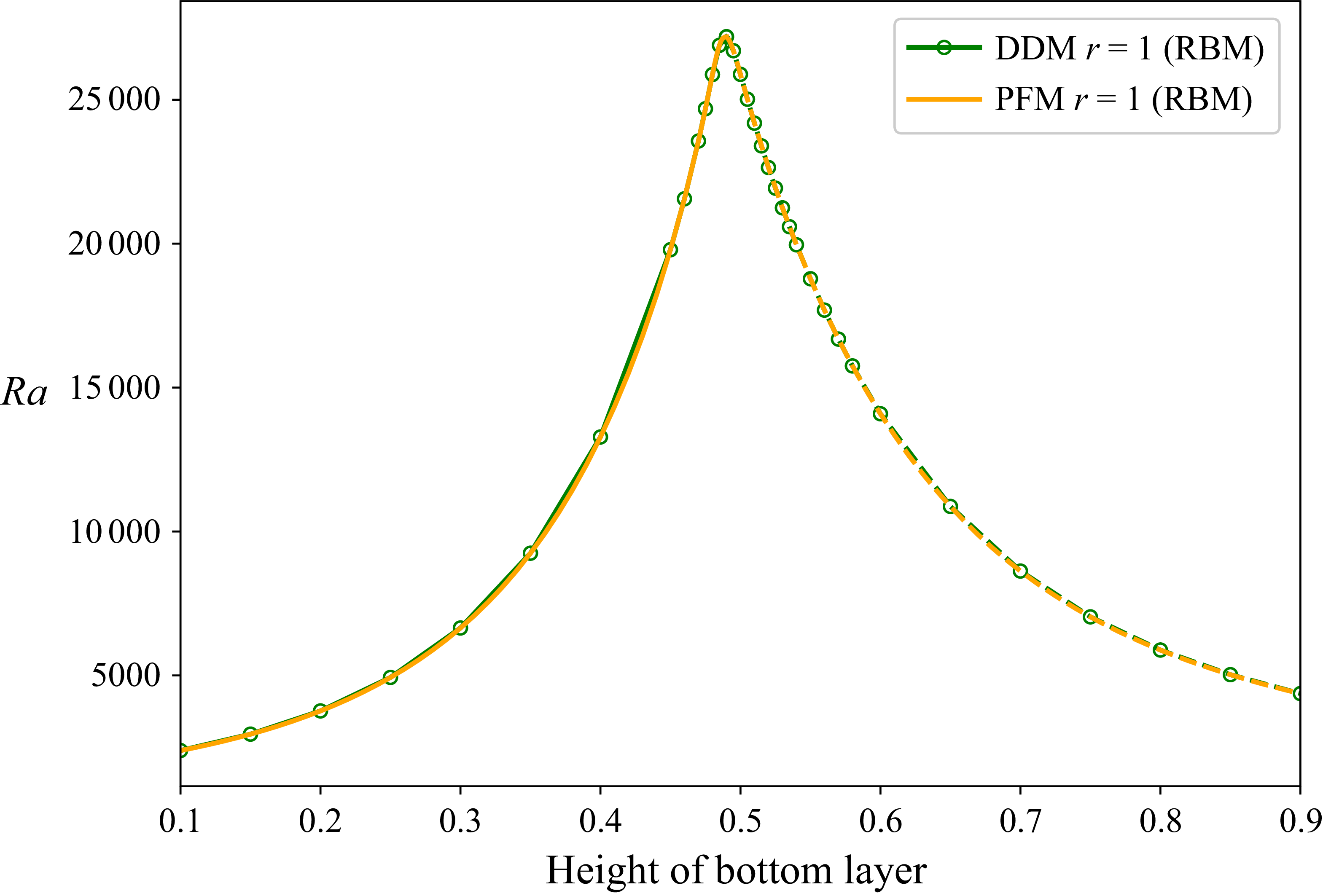
values obtained for different input wavenumbers. It is evident from the figure that an exact match is obtained between the DDM and the phase-field approaches for the prescribed conditions. The figure shows three notable regimes, whose significance will be described in the ensuing section.
A comparison between the neutral curves obtained from the DDM and the PFM for immiscible fluids.

4.3. Onset of RB convection near the UCST
Adhering to our objective of characterising RB convection onset in diffuse-interface systems, we now estimate the stability curves for different values of
 $a^*$
and
 $r$
. For the given
 $\rho \beta \alpha \, (= 0.125)$
and
 $a^*$
values, we start from a purely immiscible state, i.e.
 $r=1$
, and approach the UCST of the binary fluid combination by reducing
 $r$
to a value as low as
 $0.005$
. The results of the former have already been presented in figure 6 wherein three distinct modes have been identified at different interfacial heights. These modes are marked as TOP, BOT and OSC, respectively. The part marked as TOP corresponds to the `upper dragging mode’ wherein there is an active buoyancy-driven convection in the top layer owing to its larger thickness. The bottom layer is passively driven by the continuity of velocity and shear stress at the interface. The BOT curve represents the opposite case, wherein the bottom layer is the driver, and the top layer is driven. At intermediate heights ranging between
 $0.483$
and
 $0.53$
, the system manifests oscillatory (OSC) modes, wherein it transiently alters between a mechanically coupled state and a thermally coupled state. Here, both layers have equal propensities for primary excitation, and the system responds by oscillating between the two possible modes of coupling between the layers. In fact, on either side of this oscillatory range, the system exhibits stationary MC and TC modes depending on the properties chosen. The occurrence of oscillatory convection in a two-layer system is not always guaranteed. As mentioned earlier, a favourable combination of property ratios such as
 $\rho \beta \alpha$
being far from unity and
 $a^{*}$
being closer to unity is essential for the manifestation of oscillatory excitation.
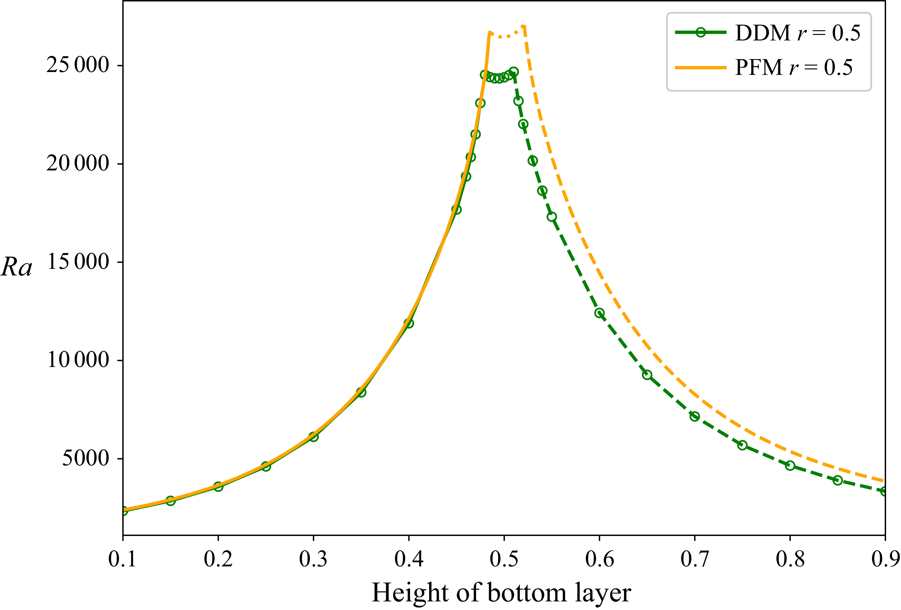
Before performing the analysis for the other values of
 $r$
, we shall briefly assess the necessity of using the phase-field formulation for the current problem. Figure 6 showed an excellent match of results between the present model and the sharp-interface approach, modelled via DDM. Taking a cue from this exact match, one might be tempted to use DDM in the binary fluid context wherein the layer properties are obtained from the equilibrium composition ((3.1)) at different temperatures. After all, the diffuse-interface thickness is much smaller than the layer heights for the range of
 $r$
considered in the present analysis. Fortunately, the answer to this dilemma is evident from figure 7, where
 $r$
is
 $0.5$
. The figure compares the phase-field model results with those of DDM, wherein the properties have been modified according to the equilibrium composition. The value of
 $r$
being
 $0.5$
implies that the fluid system is still far away from its consolute point, and yet, we see a noticeable difference between the neutral curves of PFM and DDM. The latter approach underpredicts the critical behaviour since the diffuse nature of the interface has been ignored. By correctly accounting for the dissipative effects in the small diffuse region, the PFM provides a more realistic picture of the onset behaviour. Thus, it becomes essential for any analysis involving multi-layer systems to first verify the value of
 $r$
before applying the sharp-interface assumption. Moving ahead, the characteristics of RB convection onset near the UCST are now analysed by reducing the value of
 $r$
.
A comparison between the marginal stability curves obtained from the DDM and the PFM for sparingly miscible fluids.

Neutral curves for different values of
 $r$
for
 $(\rho \beta \alpha ) = 0.125, a^{*} = 1.0$
.

Figure 8 shows the variation of the critical Rayleigh number with interfacial height for different values of
 $r$
for the fluid system with
 $\rho \beta \alpha =0.125$
and
 $a^{*}=1.0$
. In this figure, the solid, dashed and dotted lines correspond to the upper dragging, lower dragging and oscillatory modes, respectively. Note that the same convention has been followed in all the subsequent figures. It is evident from figure 8 that with the increased miscibility of fluids, the peaks of the marginal stability curves shift downward and the window for oscillatory onset becomes narrow. This shrinkage can be attributed to the change in the equilibrium composition of the two layers that increases the apparent
 $\tilde {\rho }\tilde {\beta }\tilde {\alpha }$
value, which approaches one as
 $r \rightarrow 0$
. In other words, the reduction in the contrasts of thermal expansion coefficient and viscosity between the layers does not sufficiently amplify the perturbations necessary for transitions from the MC state to the TC state and vice versa. Hence, the propensity for oscillatory convection decreases as the system approaches its consolute point. It is also evident from figure 8 that the change in equilibrium composition has different influences on the TOP and BOT modes. Recall that for the present fluid system, the values of the relevant property ratios in the immiscible limit are
 $\nu =0.5$
,
 $\beta =0.125$
,
 $\alpha =0.5$
. Thus, an increase in the system’s temperature alters these ratios such that the thermal expansivity coefficient of the bottom layer increases, and so do the kinematic viscosity and thermal diffusivity. However, the increase in the former coefficient is significant compared with the latter dissipative effects, making the bottom layer more vulnerable to perturbations. Hence, there is an effective reduction in the critical
 $Ra$
value for the BOT mode. Interestingly, the modified layer properties also lead to a marginal destabilisation of the top layer, and we observe a reduction in the peak values of the critical
 $Ra$
, which settle around
 $y_I = 0.5$
.
Figure 9 shows the critical
 $Ra$
plots for the second system of present consideration, i.e. that with
 $\rho \beta \alpha =0.125$
and
 $a^{*}=0.667$
. Here, the peaks of the marginal curves shift leftward with an increase in base temperature, i.e. with a reducing
 $r$
. Note that for the present system, in the immiscible limit, the kinematic viscosity ratio is
 $2.53$
, and any change in composition brought by the (base) temperature increase makes the bottom layer less dissipative. This, coupled with the increased thermal expansivity in the bottom layer, significantly reduces the critical
 $Ra$
for the BOT mode, as it becomes easier to establish convection there. At the same time, the change in composition stabilises the TOP layer. Nonetheless, we observe a similar reduction in the window of the oscillatory convection, and the peak value settles around the interfacial height of
 $0.5$
.
Neutral curves for different values of
 $r$
for
 $(\rho \beta \alpha ) = 0.125, a^{*} = 0.667$
.

Neutral curves for different values of
 $r$
for
 $(\rho \beta \alpha ) = 0.125, a^{*} = 1.5$
.

Lastly, we analyse the behaviour of the two-layer system with property ratio combinations,
 $\rho \beta \alpha =0.125$
and
 $a^{*}=1.5$
. Note that the kinematic viscosity ratio of the system,
 $\nu$
, is approximately 0.09875. Figure 10 shows the marginal stability curves for different values of
 $r$
. Interestingly, the curves undergo a rightward shift accompanied by a decrease in the window for oscillatory excitation in the system. The latter behaviour again relates to the increase in the apparent
 $\tilde {\rho }\tilde {\beta }\tilde {\alpha }$
value that makes the occurrence of oscillatory excitation less probable. The rightward shift essentially occurs due to the large initial disparity in the kinematic viscosities of the two layers. The change in equilibrium composition due to the base temperature increases the viscosity of the bottom layer significantly, overwhelming the influence brought in by the increase in the thermal expansion coefficient. Consequently, the BOT mode becomes more stable, requiring a larger temperature gradient to provoke instability in the system. The composition change reveals an opposite behaviour for the TOP mode making the peak
 ${Ra}$
settle close to the interfacial height of
 $0.5$
.
From the analyses of these three systems, it is evident that the propensity of a system to exhibit oscillatory convection decreases as it approaches the UCST. The equilibrium composition at these states would have a lesser disparity in the property ratios. Notably, the combination
 $\tilde {\rho }\tilde {\beta }\tilde {\alpha }$
approaches unity, and as shown by Renardy (Reference Renardy1996), such systems would become devoid of any oscillatory convection. Of course, each system comes with its own drift pattern in the stability curves, essentially determined by the thermo-physical/transport properties of the fluids.
5. Combined role of buoyancy and thermocapillarity
Following the characterisation of RB convection, we now analyse the influence of added thermocapillarity on the onset of convection in binary fluid systems. In this regard, we revert to the complete set of perturbation equations, i.e. from (3.13) to (3.17), along with the associated boundary conditions mentioned in (3.18). Despite the inclusion of Marangoni effects, the current GEP still quantifies the criticality in terms of the Rayleigh number. This is on account of
 $ {Ra}$
and
 $ {Ma}$
being linked with each other through the additional input parameter,
 $\zeta \;(= \sigma _\theta /(g\rho _2\beta _2 H^2))$
. Consequently, the fluid combinations for the present analysis are characterised by four property groups: (i) the
 $\rho \beta \alpha$
combination, which is still maintained at 0.125, (ii) the critical height ratio,
 $a^*$
, (iii) the miscibility transition parameter,
 $r$
, that is varied between 1.0 and 0.005 and (iv)
 $\zeta$
, which ranges between zero and 0.1. Before characterising the influence of the new parameter,
 $\zeta$
, we will briefly check the consistency of the Marangoni formulation.
5.1. Consistency check
A comparison between the curves of marginal stability for the RBM convection obtained from the DDM and the PFM.

Repeating the analysis performed for the RB case, we now check the ability of the current diffuse RBM formulation to mimic the sharp-interface behaviour in the immiscible limit. The comparison is once again carried out against the DDM implementation of Diwakar et al. (Reference Diwakar, Tiwari, Das and Sundararajan2014). The property combinations associated with the fluid system are
 $\rho \beta \alpha = 0.125$
,
 $r = 1.0$
,
 $a^* = 1.0$
and
 $\zeta =0.01$
. The value of
 $\epsilon /H$
is specified as
 $2 \times 10^{-4}$
to mimic the sharp-interface behaviour. Figure 11 shows an exact match between the results of the current phase-field model in the sharp-interface limit and the DDM implementation. Interestingly, the manifestation of oscillatory onset, as observed for the intermediate height range in figure 6, vanishes with the inclusion of the Marangoni effect. The reason for this behaviour is discussed in the ensuing subsection.
5.2. Rayleigh–Bénard–Marangoni convection in the immiscible limit
Schematic of interaction between buoyancy and thermocapillarity. (a) Buoyancy-driven convection in the bottom layer. (b) Buoyancy-driven convection in the top layer. Here,
 $T_C$
and
 $T_H$
are the temperatures of the cold and hot plates, respectively.

A comparison between neutral curves between RB and RBM convections. The magnitude of
 $\zeta$
corresponds to the strength of the surface tension gradients.

Apart from the favourability of property ratios such as
 $\rho \beta \alpha$
and
 $a^*$
, the Marangoni effect also plays an important role in the occurrence of oscillatory convection in immiscible two-layer systems. Nepomnyashchy & Simanovskii (Reference Nepomnyashchy and Simanovskii2004) demonstrated this influence using the silicone oil–water combination, wherein they observed an enlargement of the window for oscillatory convection with the addition of thermocapillary effects. To understand the reason behind this manifestation, we delve into the two modes of interactions between the buoyancy and thermocapillary-driven convection in a typical two-layer system. The corresponding schematics are shown in figure 12. Here, when the convection in the bottom layer is dominant, the hot plume rising in the layer creates temperature inhomogeneity along the fluid interface. Particularly, it leads to the formation of hot spots on the interface. Since the Marangoni effect drives fluid away from a hot spot, it aids the underlying buoyancy-driven convection. The system thus becomes easily destabilised, resulting in lower criticality. The scenario is exactly the opposite when the convection is dominant in the top layer. The convection rolls bring down heavier (colder) fluid from the vicinity of the top wall towards the interface, thereby making the interfacial temperature non-uniform once again. However, the Marangoni flow originating due to such cold spots opposes the bulk motion of the convection rolls in the top layer, and the corresponding critical values are higher than those observed for the pure buoyancy-driven case where
 $Ma = 0$
(Zeren & Reynolds Reference Zeren and Reynolds1972). These diverse roles of the Marangoni effect, i.e. aiding convection sometimes and inhibiting it at other times, have their signature on the oscillatory onset of convection in the system. To understand them, we now gradually increase the magnitude of the thermocapillary effect by increasing the
 $\zeta$
value of a fluid combination with property ratios
 $\rho \beta \alpha =0.125$
,
 $a^{*}=1.0$
and
 $r=1$
. Figure 13 shows the neutral curves obtained from the analysis, and it is interesting to note that the thermocapillarity does not always increase the parametric window for oscillatory onset. Evidently, the window for oscillatory convection shrinks with the increase of
 $\zeta$
from zero and mostly vanishes at around
 $\zeta =0.01$
. With a further increase in the
 $\zeta$
value, the range for oscillatory onset broadens once again. The reasons for this behaviour can be understood by extending the analysis of Renardy (Reference Renardy1996) to include the Marangoni effect. The details of the steps involved are shown in Appendix B, and for the sake of brevity, only the final equation is written as follows:
 \begin{align} \lambda ^{*} \Bigg [ \int _0^I \frac {1}{\alpha } |\hat {\theta }_1|^2 {{\rm d}y} + \int _I^1 \frac {1}{\kappa } |\hat {\theta }_2|^2 {{\rm d}y} \Bigg ] = & - \int _0^I \left ( k^2 |\hat {\theta }_1|^2 + \left | \frac {{{\rm d}}\hat {\theta }_1}{{{\rm d}y}} \right |^2 \right ) {{\rm d}y}\nonumber\\&- \int _I^1 \frac {1}{\kappa } \left ( k^2 |\hat {\theta }_2|^2 + \left | \frac {{{\rm d}}\hat {\theta }_2}{{{\rm d}y}} \right |^2 \right ) {{\rm d}y} \nonumber \\&- \frac {\lambda }{Pr_2} \frac {\varLambda _1}{k^2 Ra} \Bigg [ \int _0^I \frac {1}{\beta \alpha } \left ( k^2 |\hat {v}_1|^2 + \left | \frac {{{\rm d}}\hat {v}_1}{{{\rm d}y}} \right |^2 \right ) {{\rm d}y} \nonumber \\&+ \int _I^1 \left ( k^2 \left |\hat {v}_2\right |^2 + \left | \frac {{\rm d}\hat {v}_2} {{{\rm d}y}} \right |^2 \right ) {\mathrm{dy}} \Bigg ] \nonumber \\&- \frac {\varLambda _1}{k^2 Ra} \bigg [ \!\int _0^I\! \frac {\eta }{(\rho \beta \alpha )} \big | {\nabla^{2}\hat{v}_1} \big |^2 \!{{\rm d}y} +\! \int _I^1 \big | {\nabla^{2}\hat{v}_2} \big |^2 {{\rm d}y} \bigg ] \nonumber \\&+ \frac {\varLambda _1}{k^2 Ra} \left ( \frac {1}{\rho \beta \alpha } - 1 \right ) \frac {{{\rm d}}{\hat {v}^*}_2}{{{\rm d}y}} \frac {{\rm d}^2\hat {v}_2}{{{\rm d}y}^2}\bigg |_{y=I} \nonumber \\&- \varLambda _1 \frac {1}{(\rho \beta \alpha )} \zeta \hat {\theta }_2 \frac {{{\rm d}}{\hat {v}^*}_2}{{{\rm d}y}}\bigg |_{y=I}. \end{align}
At this juncture, it is worth remembering that the leading eigenvalue of the system need not be complex if it is non-self-adjoint. Conversely, if the eigenvalue is complex, the system has to be non-self-adjoint. Hence, the criteria of
 $\rho \beta \alpha \gg 1.0$
or
 $\rho \beta \alpha \ll 1.0$
provided by Renardy (Reference Renardy1996) for non-self-adjointness of an RB system form a necessary, but not a sufficient, condition for the occurrence of oscillatory onset (Diwakar et al. Reference Diwakar, Tiwari, Das and Sundararajan2014). In a similar sense, the present discussions focus on the additional impact of Marangoni effects on the necessary condition for oscillations. It is evident that the last two terms containing velocity derivatives at the interface in (5.1) contribute to the non-self-adjointness. Correspondingly, one can infer that when
 $\rho \beta \alpha$
is unity and when the thermocapillarity is absent, the system will exhibit a non-oscillatory (steady) onset of convection. It is also understandable that the present system (figure 13) would be non-self-adjoint simply by the virtue of favourable
 $\rho \beta \alpha$
( = 0.125), when the value of
 $\zeta$
is zero. However, for a non-trivial value of
 $\zeta$
, which is approximately
 $0.01$
in the current case, the thermocapillarity appears to nullify the
 $\rho \beta \alpha$
influence. This results in the manifestation of a stationary onset at all interfacial heights, as observed in figure 11. When
 $\zeta$
deviates from this value, the system has the propensity to exhibit oscillatory convection.
A manifestation of these attributes can be observed in the experimental investigation of Degen et al. (Reference Degen, Colovas and Andereck1998). Their trials on the Fluorinert FC70–47v10 silicone oil combination, with
 $\rho \beta \alpha =0.776$
and
 $\zeta \approx 0.031$
, did not show any oscillatory onset of convection. However, the linear stability study by Renardy & Stoltz (Reference Renardy and Stoltz2000) on the same fluid pair predicted the time-dependent behaviour when they considered Marangoni effects to be negligible (i.e.
 $\zeta =0$
). Interestingly, in the same work of Degen et al. (Reference Degen, Colovas and Andereck1998), the second fluid pair consisting of silicone oil 47v2–water (
 $\rho \beta \alpha =0.375$
), whose
 $\zeta$
is approximately
 $0.069$
, showed the oscillatory behaviour at the convection onset. Nepomnyashchy & Simanovskii (Reference Nepomnyashchy and Simanovskii2004), through their linear analysis, attributed the oscillatory onset to the presence of the Marangoni effect. Thus, the dual role of Marangoni effects in suppressing the oscillatory onset at times and enhancing it at other times is clearly evident.
Marginal stability curves for different values of
 $r$
for
 $\zeta =0.01$
,
 $(\rho \beta \alpha )=0.125$
. A decrease in the value of
 $r$
represents more soluble mixtures.

5.3. Rayleigh–Bénard–Marangoni convection in the binary fluid system
Moving away from the immiscible consideration, we will now discuss the onset characteristics of RBM convection in binary fluids. Understandably, both the coefficient of surface tension and its gradient with respect to temperature reduce to zero when the system’s base temperature approaches the UCST (
 $r\to 0$
). Despite this behaviour, the Marangoni effect still influences the flow onset pattern in the system, at least for moderate values of
 $r$
. In order to understand these influences, the Marangoni effect is modelled presently by considering the mixing energy to be a linear function of temperature, i.e.
 $\varLambda = \varLambda _0 + (\partial \varLambda / \partial \theta ) \theta$
. The decrease in the magnitude of the mixing energy with the increase in interfacial thickness, i.e. with reducing
 $r$
, suitably models the dwindling behaviour of the Marangoni effect near the UCST.
It is worth recalling that in the case of RB convection, the window of oscillatory instability invariably shrinks with the decrease in
 $r$
value. With the inclusion of the Marangoni effect, we will now see a completely different manifestation. Figures 14 and 15 show the neutral curves for different values of
 $r$
at two constant
 $\zeta$
values. Note that the first system (figure 14) with
 $\rho \beta \alpha =0.125$
,
 $a^{*}=1.0$
and
 $\zeta =0.01$
has nearly no oscillatory transition in the pure immiscible state (
 $r=1$
). With the decrease in
 $r$
, the window for oscillatory onset interestingly increases until a point. However, closer to the UCST, i.e. for very small values of
 $r$
, the oscillatory window narrows as the Marangoni effect becomes feeble. In fact, in this region, the system exhibits behaviour similar to that observed for RB convection.
The second system (figure 15) with
 $\rho \beta \alpha =0.125$
,
 $a^{*}=1.0$
and
 $\zeta =0.1$
possesses a relatively large window of oscillatory onset in the immiscible limit. The oscillatory window shrinks with the decrease in
 $r$
. In fact, it completely vanishes at
 $r=0.1$
. However, with the further reduction in
 $r$
, the oscillatory window does not reappear as the Marangoni effect dwindles for the lower values of
 $r$
.
Interestingly, these two systems with
 $\zeta =0.01$
and
 $\zeta =0.1$
have manifested different behaviours. In the first case, we see that the window for oscillatory convection first increases and then decreases with the reduction of
 $r$
. The situation in the second case leads to a monotonic reduction of the oscillatory window. The reason for this divergent behaviour can be understood by revisiting (5.1). As mentioned in the previous subsection, the onset of oscillatory convection is governed by two interfacial terms containing
 $(( {1}/({\rho \beta \alpha }))-1)$
and
 $\zeta$
, respectively. With the increase of interfacial thickness, i.e. with reducing
 $r$
, the influences of both these terms dwindle. However, the Marangoni effect weakens much faster and plays no role for small
 $r$
values. This is evident from figure 16 wherein the neutral curves for different values of
 $\zeta$
are identical with the RB case. For moderate
 $r$
values, nevertheless, the terms compete to manifest diverse behaviour. In the first case with
 $\zeta =0.01$
, the
 $(({1}/({\rho \beta \alpha }))-1)$
term and the
 $\zeta$
term seem to nullify each other at
 $r=1$
. With the reduction in
 $r$
, the increased solubility of fluids in each other reduces the disparities in the layer properties. As a result,
 $\tilde {\rho }\tilde {\beta }\tilde {\alpha }$
increases and approaches one, and its influence on the oscillatory onset of convection weakens. At the same time, the influence of the
 $\zeta$
term is also modified as it is multiplied by
 ${1}/({\rho \beta \alpha })$
. Interestingly, the interplay between these effects still leads to the occurrence of an oscillatory onset for moderate
 $r$
values. However, at very low values of
 $r$
, the oscillatory window narrows down as the interfacial thickness increases and the mixing energy density reduces.
We can observe from these discussions that the changing solubilities of the fluids can affect the onset characteristics in both ways. It can either inhibit or expand the oscillatory regime. In order to put things under proper perspective, we now take a combination of data as shown in figure 17. Here, the system with
 $\zeta =0.01$
has almost no oscillatory onset in the immiscible limit, whereas it manifests a sizable window with the reduction of
 $r$
. On the other hand, the system with
 $\zeta =0.1$
exhibits oscillatory onset in the immiscible limit and becomes completely non-oscillatory for
 $r$
values less than
 $0.1$
.
Marginal stability curves for different values of
 $r$
for
 $\zeta =0.1$
,
 $(\rho \beta \alpha )=0.125$
. A decrease in the value of
 $r$
represents more soluble mixtures.

A comparison between the marginal stability curves for the RB and RBM convections closer to the critical temperature.

Marginal stability curves for different values of
 $\zeta$
and
 $r$
for
 $(\rho \beta \alpha )=0.125$
. The combination
 $(\zeta , r) = (0.01, 1)$
shows almost no oscillatory onset behaviour, and
 $(\zeta , r) = (0.1, 0.1)$
shows complete non-oscillatory onset.

Marginal stability curves for different values of
 $\zeta$
and
 $r$
for
 $(\rho \beta \alpha ) = 0.25, 0.5$
. For (a)
 $\rho \beta \alpha = 0.25$
, the combinations
 $(\zeta , r) = \{(0.01, 1), (0.02, 0.5), (0.1, 0.1)\}$
, and for (b)
 $\rho \beta \alpha = 0.5$
,
 $(\zeta , r) = \{(0.01, 1), (0.1, 0.1)\}$
show the non-oscillatory onset behaviour.

It is worth remembering from the previous section that the nullification of the oscillatory regime in the completely immiscible limit occurs at
 $\zeta \approx 0.01$
. However, it is premature to state that
 $r\zeta$
plays the same role as
 $\zeta$
in the pure immiscible state (
 $r=1.0$
) without developing an expression similar to (5.1) for the diffuse-interface consideration. Nevertheless, we have been able to verify this claim for other systems with
 $(\rho \beta \alpha ) =$
0.25 and 0.5, as shown in figure 18. One can observe that the onset nature of the system becomes completely time-independent when
 $r\zeta \approx 10^{-2}$
.
6. Conclusion
The analysis of the onset of RBM convection in binary fluids closer to the UCST via a diffuse-interface approach reveals interesting features. Firstly, it is evident that the phase-field approach is potent enough to reveal the sharp-interface features in the truly immiscible limit exactly. Secondly, the analysis reveals that the effect of the actual diffused nature of the interface is too significant and cannot be ignored in the vicinity of the critical point. Thirdly, the propensity of the system to exhibit oscillatory convection decreases as it approaches the UCST. The equilibrium composition at these states would have a lesser disparity in the property ratios. Particularly, the combination
 $\tilde {\rho }\tilde {\beta }\tilde {\alpha }$
approaches unity, and as shown by Renardy (Reference Renardy1996), such systems would become devoid of any oscillatory convection. Of course, each system would come with its own drift pattern in the stability curves, essentially determined by the thermo-physical/transport properties of the fluids. The current analysis of a two-layer RBM convection with a diffuse-interface model provides some interesting information. In the pure immiscible limit, the Marangoni effect plays the dual role of suppressing the oscillatory convection in some range and enhancing it elsewhere. This is essentially due to the contribution played by two boundary terms, one involving
 $ (({1}/({\rho \beta \alpha })) - 1 )$
and the other involving the non-dimensional surface tension gradient (
 $\zeta$
). The interplay between these terms can make the system non-self-adjoint and possibly make it exhibit oscillatory excitation. The role of solubility is quite intriguing as it acts in unison with the interfacial tension term to make the system either self-adjoint or non-self-adjoint. Thus, it comes with its own dual role, a behaviour not particularly evident for the RB instability. These interesting facets can be further explored in the future with the help of full non-linear simulations that would employ the present phase-field formulation.
Supplementary material
Supplementary material is available at https://doi.org/10.1017/jfm.2026.11206.
Declaration of interests
The authors report no conflict of interest.
Appendix A. Recalculating spatial derivatives
 $g(y)$
is the mapping function and
 $\Xi$
is the any pertinent dependent variable.
 \begin{align} \frac {\mathrm{d} \varXi }{\mathrm{d}\tilde {y}} &= \frac {1}{g^{\prime }} \frac {\mathrm{d}\varXi }{\mathrm{d} y}\nonumber\\ \frac {{\rm d}^2 \varXi }{\mathrm{d}\tilde {y}^2} &= \frac {1}{(g^{\prime })^2} \frac {{\rm d}^2 \varXi }{\mathrm{d}y^2} - \frac {g^{\prime \prime }}{(g^{\prime })^3} \frac {\mathrm{d}\varXi }{\mathrm{d} y}\nonumber\\ \frac {{\rm d}^3 \varXi }{\mathrm{d}\tilde {y}^3} &= \frac {1}{(g^{\prime })^3} \frac {{\rm d}^3 \varXi }{\mathrm{d} y^3} - \frac {3g^{\prime \prime }}{(g^{\prime })^4} \frac {{\rm d}^2 \varXi }{\mathrm{d} y^2} - \frac {g^{\prime } g^{\prime \prime \prime } - 3(g^{\prime \prime })^2}{(g^{\prime })^5} \frac {\mathrm{d}\varXi }{\mathrm{d} y}\nonumber\\ \frac {{\rm d}^4\varXi }{\mathrm{d}\tilde {y}^4} &= \frac {1}{(g^{\prime })^4} \frac {{\rm d}^4 \varXi }{\mathrm{d} y^4} - \frac {6g^{\prime \prime }}{(g^{\prime })^5} \frac {{\rm d}^3 \varXi }{\mathrm{d} y^3} - \frac {4g^{\prime } g^{\prime \prime \prime } - 15(g^{\prime \prime })^2}{(g^{\prime })^6} \frac {{\rm d}^2 \varXi }{\mathrm{d} y^2}\nonumber \\ & - \frac {(g^{\prime})^2 g^{\prime \prime \prime \prime } - 10g^{\prime}g^{\prime \prime }g^{\prime \prime \prime } + 15(g^{\prime \prime })^3}{(g^{\prime })^7} \frac {\mathrm{d}\varXi }{\mathrm{d}y}\end{align}
Appendix B. Revisiting the theory to predict oscillatory onset in RBM convection
The equations governing the evolution of the perturbations, in dimensionless form, are
 \begin{align} \frac {\partial \boldsymbol{u}^{\prime }_1}{\partial t} &= -\frac {1}{\rho } Pr_2 \boldsymbol{\nabla } p^{\prime }_1 + Ra Pr_2 \beta \theta ^{\prime }_1 \boldsymbol{1}_y + Pr_2\nu {\nabla }{^2}\boldsymbol{u}^{\prime }_1, \\[-10pt] \nonumber \end{align}
 \begin{align} \frac {\partial \boldsymbol{u}^{\prime }_2}{\partial t} &= -Pr_2 \boldsymbol{\nabla } p^{\prime }_2 + Ra Pr_2 \theta ^{\prime }_2 \boldsymbol{1}_y + Pr_2{\nabla }{^2} \boldsymbol{u}^{\prime }_2, \\[-10pt] \nonumber \end{align}
 \begin{align} \frac {\partial \theta ^{\prime }_1}{\partial t} &= -v^{\prime }_1\varLambda _1 + \alpha {\nabla }{^2} \theta ^{\prime }_1, \\[-10pt] \nonumber \end{align}
 \begin{align} \frac {\partial \theta ^{\prime }_2}{\partial t} &= -v^{\prime }_2\varLambda _2 + {\nabla }{^2}\theta ^{\prime }_2, \\[9pt] \nonumber \end{align}
where we have chosen the same scales as before to non-dimensionlise the equations. Operating with
 $\boldsymbol{1}_y \boldsymbol{\cdot }\boldsymbol{\nabla } \times \boldsymbol{\nabla } \times$
, the momentum equations take the following form:
 \begin{align} \frac {\partial }{\partial t} \big ({\nabla }{^2} v^{\prime }_1\big ) &= Ra Pr_2\beta \frac {\partial ^2\theta ^{\prime }_1}{\partial x^2} + Pr_2\nu {\nabla }{^4} v^{\prime }_1, \\[-10pt] \nonumber \end{align}
 \begin{align} \frac {\partial }{\partial t} \big ({\nabla }{^2} v^{\prime }_2\big ) &= Ra Pr_2 \frac {\partial ^2\theta ^{\prime }_2}{\partial x^2} + Pr_2{\nabla }{^4} v^{\prime }_2. \end{align}
Following the standard normal mode expansion, i.e. the perturbations being proportional to
 $\exp (\lambda t + \mathrm{i}kx)$
, as mentioned in (3.12), the set of governing equations can be written as
 \begin{align} \frac {\lambda }{Pr_2} \left (-k^2+\frac {{\rm d}^2}{\mathrm{d}y^2}\right ) \hat {v}_1 &= -k^2 Ra\beta \hat {\theta }_1 + \nu \left (-k^2+\frac {{\rm d}^2}{\mathrm{d}y^2}\right )^2 \hat {v}_1, \end{align}
 \begin{align} \frac {\lambda }{Pr_2} \left (-k^2+\frac {{\rm d}^2}{\mathrm{d}y^2}\right ) \hat {v}_2 &= -k^2 Ra \hat {\theta }_2 + \left (-k^2+\frac {{\rm d}^2}{\mathrm{d}y^2}\right )^2 \hat {v}_2, \end{align}
 \begin{align} \lambda \hat {\theta }_1 &= - \hat {v}_1\varLambda {_1} + \alpha \left (-k^2+\frac {{\rm d}^2}{\mathrm{d}y^2}\right ) \hat {\theta }_1, \end{align}
 \begin{align} \lambda \hat {\theta }_2 &= - \hat {v}_2 \varLambda _2 + \left (-k^2+\frac {{\rm d}^2}{\mathrm{d}y^2}\right ) \hat {\theta }_2. \end{align}
We now multiply (B9) and (B10) with
 $ {\hat {\theta }^{*}_1}/{\alpha }$
and
 ${\hat {\theta }^{*}_2}/{\kappa }$
, respectively, where
 $\hat {\theta }^{*}_1$
and
 $\hat {\theta }^{*}_2$
are the complex conjugates of
 $\hat {\theta }_1$
and
 $\hat {\theta }_2$
. Subsequently, we add the complex conjugates of the resulting equations and obtain the following relationship:
 \begin{align} \lambda ^{*} \left [\int _0^I \frac {1}{\alpha } |\hat {\theta }_1|^2 \mathrm{d}y + \int _I^1 \frac {1}{\kappa } |\hat {\theta }_2|^2 \mathrm{d}y \right ] &= \int _0^I \hat {\theta }_1 \left (-k^2+\frac {{\rm d}^2}{\mathrm{d}y^2}\right ) {\hat {\theta }^*}_1 \mathrm{d}y\nonumber\\& \quad + \int _I^1 \frac {1}{\kappa } \hat {\theta }_2 \left (-k^2+\frac {{\rm d}^2}{\mathrm{d}y^2}\right ) {\hat {\theta }^*}_2 \mathrm{d}y \nonumber \\& \quad - \int _0^I \frac {1}{\alpha }\varLambda _1 {\hat {v}^*}_1\hat {\theta }_1 \mathrm{d}y - \int _I^1 \varLambda _1 {\hat {v}^*}_2\hat {\theta }_2 \mathrm{d}y, \end{align}
where
 $\varLambda _1={\varLambda _2}/{\kappa }$
.
In a similar way, we multiply (B7) and (B8) with
 ${\varLambda _1 \hat {v}_1^{*}}/{\alpha }$
and
 $\varLambda _1\hat {v}_2^{*}$
, respectively, where
 $\hat {v}^{*}_1$
and
 $\hat {v}^{*}_2$
are the complex conjugates of
 $\hat {v}_1$
and
 $\hat {v}_2$
. After eliminating the cross products such as
 $\hat {v}_1^{*}\hat {\theta }_1$
and
 $\hat {v}_2^{*}\hat {\theta }_2$
from the momentum and energy equations, we obtain
 \begin{align} \lambda ^{*} \Bigg [ \int _0^I \frac {1}{\alpha } |\hat {\theta }_1|^2 {{\rm d}y} + \int _I^1 \frac {1}{\kappa } |\hat {\theta }_2|^2 {{\rm d}y} \Bigg ] = & - \int _0^I \left ( k^2 |\hat {\theta }_1|^2 + \left | \frac {{\rm d}\hat {\theta }_1}{{{\rm d}y}} \right |^2 \right ) {{\rm d}y}\nonumber\\&- \int _I^1 \frac {1}{\kappa } \left ( k^2 |\hat {\theta }_2|^2 + \left | \frac {{\rm d}\hat {\theta }_2}{{{\rm d}y}} \right |^2 \right ) {{\rm d}y} \nonumber \\&- \frac {\lambda }{Pr_2} \frac {\varLambda _1}{k^2 Ra} \Bigg [ \int _0^I \frac {1}{\beta \alpha } \left ( k^2 |\hat {v}_1|^2 + \left | \frac {{\rm d}\hat {v}_1}{{{\rm d}y}} \right |^2 \right ) {{\rm d}y} \nonumber \\&+ \int _I^1 \left ( k^2 \left |\hat {v}_2\right |^2 + \left | \frac {{\rm d}\hat {v}_2} {{{\rm d}y}} \right |^2 \right ) {{{\rm d}y}} \Bigg ] \nonumber \\&- \frac {\varLambda _1}{k^2 Ra} \bigg [\! \int _0^I \!\frac {\eta }{(\rho \beta \alpha )} \big | {\nabla^{2}\hat{v}_1} \big |^2 {{\rm d}y} \!+\! \int _I^1 \big | {\nabla^{2}\hat{v}_2} \big |^2 {{\rm d}y} \bigg ] \nonumber \\&+ \frac {\varLambda _1}{k^2 Ra} \left ( \frac {1}{\rho \beta \alpha } - 1 \right ) \frac {{\rm d}{\hat {v}^*}_2}{{{\rm d}y}} \frac {{\rm d}^2\hat {v}_2}{{{\rm d}y}^2}\bigg |_{y=I} \nonumber \\&- \varLambda _1 \frac {1}{(\rho \beta \alpha )} \zeta \hat {\theta }_2 \frac {{\rm d}{\hat {v}^*}_2}{{{\rm d}y}}\bigg |_{y=I}. \end{align}
The boundary conditions that arise from the integration-by-parts with respect to
 $y$
are (i)
 $\hat {v}_1 = \hat {v}_2 = 0$
(non-deformable interface), (ii)
 ${{\rm d} \hat {v}_1}/{{{\rm d}y}} = {{\rm d} \hat {v}_2}/{{{\rm d}y}}$
(derived from continuity of tangential velocity), (iii)
 $\eta ( {{\rm d}^2 \hat {v}_1}/{{{\rm d}y}^2}) = ( {{\rm d}^2 \hat {v}_2}/{{{\rm d}y}^2}) - k^2 Ma \hat {\theta }_1$
(continuity of shear stress), (iv)
 $\hat {\theta }_1 = \hat {\theta }_2$
(continuity of temperature) and (v)
 $\kappa ({{{\rm d}} \hat {\theta }_1}/{{{\rm d}y}}) = {{{\rm d}} \hat {\theta }_2}/{{{\rm d}y}}$
(continuity of heat flux at the interface).