



1. Introduction
Boundary slip is critical for the interfacial flow and transport phenomena in micro-/nanofluidics (Sparreboom et al. Reference Sparreboom, Van Den Berg and Eijkel2009; Qin et al. Reference Qin, Yuan, Zhao, Xie and Liu2011; Secchi et al. Reference Secchi, Marbach, Niguès, Stein, Siria and Bocquet2016; Cai et al. Reference Cai, Li and Bian2025), and has been widely used in drag reduction (Huang et al. Reference Huang, Lv and Duan2019; Li et al. Reference Li, Ji, Duan, Lan, Zhang and Lv2020b
; Wang et al. Reference Wang, Wang and Liu2022), energy harvesting (Rankin & Huang Reference Rankin and Huang2016; Long et al. Reference Long, Zhao, Kuang, Liu and Liu2020) and efficient lubrication (Aurelian et al. Reference Aurelian, Patrick and Mohamed2011; Yan et al. Reference Yan, Song, Zheng, Cui, Wang and Xu2024). The observation of boundary slip can be traced back to the time of Leonardo da Vinci (Xia Reference Xia2024), and Navier introduced the slip length
 $b$
to quantitatively describe the slippage (Navier Reference Navier1822).
Apparent boundary slip has been observed on hydrophobic surfaces (Feuillebois et al. Reference Feuillebois, Bazant and Vinogradova2009; Rothstein Reference Rothstein2010), where the slip length correlates with the contact angle of the solid surface (Ou et al. Reference Ou, Perot and Rothstein2004; Davies et al. Reference Davies, Maynes, Webb and Woolford2006; Huang et al. Reference Huang, Sendner, Horinek, Netz and Bocquet2008; Bouzigues et al. Reference Bouzigues, Tabeling and Bocquet2008; Lee & Kim Reference Lee and Kim2014). The obvious slip at the hydrophobic surfaces has been attributed to the presence of surface bubbles, which strongly reduce the solid–liquid (SL) friction since the gas phase is shear-free due to the negligible viscosity of air (Tyrrell & Attard Reference Tyrrell and Attard2001; Lauga & Stone Reference Lauga and Stone2003; Haase et al. Reference Haase, Wood, Lammertink and Snoeijer2016). Interfaces covered by surface bubbles have considerable potential for surface cleaning (Liu & Craig Reference Liu and Craig2009), flotation (Wu et al. Reference Wu, Nesset, Masliyah and Xu2012) and nanomaterial engineering (Berkelaar et al. Reference Berkelaar, Zandvliet and Lohse2013). Another widely used approach is to trap air pockets within microstructured surfaces on hydrophobic surfaces (Choi et al. Reference Choi, Ulmanella, Kim, Ho and Kim2006; Ming et al. Reference Ming, Jian, Chunxia, Xiaokang and Lan2011). These gas cavities, stabilised by Laplace pressure, form macroscale liquid–gas (LG) interfaces that significantly reduce drag and promote interfacial transport (Feuillebois et al. Reference Feuillebois, Bazant and Vinogradova2009; Karatay et al. Reference Karatay, Haase, Visser, Sun, Lohse, Tsai and Lammertink2013; Lee et al. Reference Lee, Charrault and Neto2014b ).
Thus, maximising the bubble area at a surface could help to enhance the flow and transport phenomena in confinement according to previous studies. Besides, precise measurement of the LG interface slippage is crucial to understanding the relevant transport phenomena. Over the past few decades, various experimental techniques have been developed to characterise the slip properties of LG interfaces (Lee et al. Reference Lee, Choi and Kim2016), including particle image velocimetry (Bouzigues et al. Reference Bouzigues, Tabeling and Bocquet2008; Li et al. Reference Li, Li, Tan, Wang, Huang, Xiang, Lv and Duan2020a
), atomic force microscopy (Nizkaya et al. Reference Nizkaya, Dubov, Mourran and Vinogradova2016), capillary techniques (Lohse & Zhang Reference Lohse and Zhang2015) and rheometry (Choi & Kim Reference Choi and Kim2006; Truesdell et al. Reference Truesdell, Mammoli, Vorobieff, van Swol and Brinker2006; Lee et al. Reference Lee, Choi and Kim2008). However, device-to-device differences often result in large variations in the measured slip length. For instance, the flow profile in a hydrophobic microchannel shows an apparent slip velocity at the solid boundary, with micro-particle image velocimetry measurements indicating slip lengths of the order of tens of nanometres (Bouzigues et al. Reference Bouzigues, Tabeling and Bocquet2008), while Lee et al. reported a giant slip length of 185
 ${\unicode[Arial]{x03BC}} \mathrm{m}$
by controlling the pitch and gas fraction on a hydrophobic surface using a rheometer system (Lee et al. Reference Lee, Choi and Kim2008).
These inconsistencies arise from two primary challenges. First, the stochastic formation of surface bubbles is difficult to control (Zhang et al. Reference Zhang, Chan, Wang and Maeda2013; Lohse & Zhang Reference Lohse and Zhang2015), resulting in variations of experimental results in interfacial properties such as contact angle, surface roughness and curvature-dependent surface tension (Seddon & Lohse Reference Seddon and Lohse2011; An et al. Reference An, Liu and Craig2015). This heterogeneity in surface chemistry causes uncertainties in slip length measurements and hinders reliable electrokinetic analysis (Haase et al. Reference Haase, Wood, Lammertink and Snoeijer2016; Li et al. Reference Li, Jing, Pan, Bhushan and Zhao2016; Verschoof et al. Reference Verschoof, van der Veen, Sun and Lohse2016). Haase et al. (Reference Haase, Wood, Lammertink and Snoeijer2016) found that the effective slip length over a bubble mattress reaches a maximum at a small protrusion angle (
 $\sim$
9
 $^\circ$
), while Li et al. (Reference Li, Jing, Pan, Bhushan and Zhao2016) reported that the slip length increased from 8 to 512 nm as the nanobubble coverage increased from
 $1.7\,\%$
to
 $50.8\,\%$
, while contact angle decreased from 42.8
 $^\circ$
to 16.6
 $^\circ$
.
Second, for trapped air pockets in micro- and nanoscale surface structures, boundary slip is highly sensitive to the geometry and physicochemical properties of the SL interface, including surface topography (Ou et al. Reference Ou, Perot and Rothstein2004; Davies et al. Reference Davies, Maynes, Webb and Woolford2006), wettability (Wang et al. Reference Wang, Bhushan and Maali2009; Lee & Kim Reference Lee and Kim2014) and the gas fraction retained in surface features (Lee et al. Reference Lee, Choi and Kim2008; Hu et al. Reference Hu, Wang, Ren, Bao, Priezjev and Wen2018). In addition, external perturbations such as pressure (Lv et al. Reference Lv, Xue, Shi, Lin and Duan2014), air diffusion (Bobji et al. Reference Bobji, Kumar, Asthana and Govardhan2009; Poetes et al. Reference Poetes, Holtzmann, Franze and Steiner2010) and evaporation (Reyssat et al. Reference Reyssat, Yeomans and Quéré2008; Tsai et al. Reference Tsai, Lammertink, Wessling and Lohse2010) can destabilise the LG interface by overcoming the energy barrier, thereby degrading the slip effect (Lv et al. Reference Lv, Xue and Duan2016). For instance, Karatay et al. used microcavities in a microfluidic channel to trap microbubbles and found that the effective slip length reached a maximum at an optimal protrusion angle around 10
 $^\circ$
, leading to drag reduction of up to
 $23\,\%$
. However, beyond a critical angle (
 $\sim$
62
 $^\circ$
), the slip length became negative, indicating increased flow resistance (Karatay et al. Reference Karatay, Haase, Visser, Sun, Lohse, Tsai and Lammertink2013). Lee & Kim (Reference Lee and Kim2014) also showed that significant slip only occurred on surfaces with short, sparsely distributed and strongly hydrophobic protrusions. Moreover, Lv et al. (Reference Lv, Xue, Shi, Lin and Duan2014) demonstrated that shear stress could deform air pockets and alter their stability, and that high operating pressures tend to collapse the pockets and suppress interfacial slip. These findings highlight the necessity for a platform that can characterise the intrinsic slip behaviour of LG interfaces under shear-free, stable and reproducible conditions.
In this work, we investigate the ionic diffusion currents through a static bubble thin liquid film with a solid–liquid–gas interface, uncovering the slip-amplified effective surface charge density and intrinsic slip length at the LG interface under the influence of ionic surfactants. Unlike pressure-driven flow, the liquid-film thickness remains constant under diffusio-osmosis, with a known and reproducible LG interface. We introduced a single microbubble in a circular glass capillary, forming a thin liquid film between the bubble and the capillary wall (Ma et al. Reference Ma, Sun, Duan, Van Den, Albert, Jan and Xie2020; Niu et al. Reference Niu, Ma and Xie2024). Under a wide range of salt concentration gradients across the bubble in various surfactant concentrations, we measured the conductance and diffusion currents.
Our results show the effective surface charge density at the LG interface increases with surfactant concentration and reaches a maximum near
 $10^{-1}$
mM, then decreases at higher concentrations. We attribute the initial increase to enhanced intrinsic surface charge from adsorbed surfactants, and the subsequent decrease to increased interfacial friction at high adsorption density, consistent with our theoretical analysis and prior molecular simulations (Joly et al. Reference Joly, Detcheverry and Biance2014; Yan et al. Reference Yan, Niu, Sun and Xie2025).
We develop an analytical model based on adsorption isotherms and Marangoni stress to quantify surfactant-induced variations in slip length at the LG interface. The model captures diffusion currents under osmotic driving and enables extraction of the intrinsic slip length as a function of surfactant concentration. The slip length remains approximately
 $3 \ {\unicode[Arial]{x03BC}} \mathrm{m}$
below
 $10^{-2}$
mM and decreases sharply at higher concentrations. By maximising the LG interfacial area using a confined bubble, we significantly enhance flow and mass transport within the film nanochannel. This configuration increases osmotic energy conversion compared with non-slipping solid interfaces and provides a strategy to exploit soft, slipping boundaries to boost nanoscale transport.
2. Experimental set-up
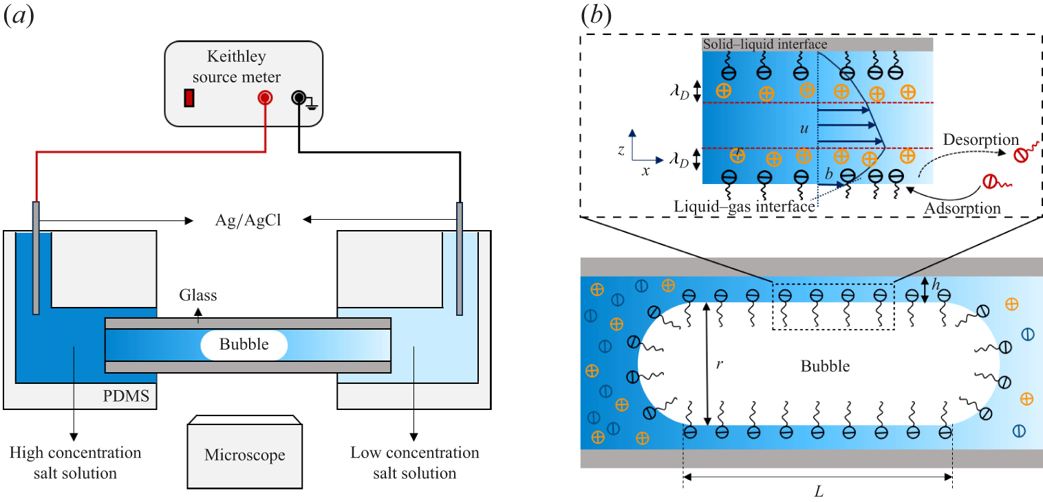
Figure 1(a) illustrates the experimental set-up. A circular glass capillary is embedded in a polydimethylsiloxane (PDMS) microfluidic chip fabricated by standard photolithography. A rectangular PDMS microchannel (200 μm wide, 400 μm high) serves as both a loading chamber and a connection port, enabling gas and electrolyte injection, inserting two Ag/AgCl electrodes, and rapid solution exchange to establish the salt concentration gradient across the bubble. We manually generated a single microbubble by injecting nitrogen gas (99.99 %) into the microchannels by using a syringe pump. Consequently, we guided the bubble into the circular glass capillary (300 μm inner diameter). The microbubble occupies most of the capillary cross-section, leaving a thin liquid film between the bubble and the capillary wall (figure 1 b).
Schematic of the experimental set-up. (a) Experimental set-up includes a bubble control system, microscope optical imaging system and electrical measurement system. (b) Geometry in the region of the LG interface in detail.

The bubble size remains constant over 12 h, due to the low solubility of nitrogen gas in water. As previously reported (Ma et al. Reference Ma, Sun, Duan, Van Den, Albert, Jan and Xie2020), the film thickness in equilibrium state is governed by the balance between the Laplace pressure of the bubble meniscus and the disjoining pressure of the thin liquid film, considering van der Waals force, electrostatic repulsion between interfaces and surface wettability. We pretreated the glass capillary by sequentially injecting 30 % hydrogen peroxide and 100 mM sodium hydroxide for 30 and 60 minutes, respectively. We then rinsed the capillary with NaCl solution for at least 30 minutes. To measure the ionic diffusion current, we established a salt concentration gradient across the bubble. First, we filled the microchannels and generated a bubble using a low-concentration solution (
 $C_{\textit{min}} = 1$
mM). We then injected a high-concentration solution (
 $C_{\textit{max}}$
) from the left-hand side to push the bubble into the capillary and establish the concentration gradient. We varied
 $C_{\textit{max}}$
from 10 to 200 mM for current measurements.
We measured the conductance of the bubble liquid film using both triangular voltage sweeps and electrochemical impedance spectroscopy (EIS) (Li et al. Reference Li2025), enabling us to infer the film thickness from its conductance in NaCl solution. We applied a triangular voltage sweep (
 $\pm 0.5$
V) within the electrochemical window to avoid concentration polarisation and limiting-current effects (Schoch et al. Reference Schoch, Han and Renaud2008). A Keithley 6430 source meter generated the waveform at a quasi-static scan frequency of
 $\sim 0.435$
Hz. The measured response remained in the resistive regime below
 $\sim$
100 Hz, thus avoiding the capacitive effects as indicated by EIS results.
The EIS was performed with a CH Instruments 600E electrochemical workstation. Two Ag/AgCl electrodes were inserted into side ports of the PDMS chip (figure 1
a) to complete the measurement circuit. We first characterised the electrical resistance of the system without a bubble (
 $R_{nb}$
), and then measured the resistance after introducing a bubble (
 $R_{b}$
). This resistance change enabled us to derive the electrical resistance of the film nanochannel as
 $R_{f}=R_{b}-R_{nb}$
. The resistance of the bubble meniscus is much smaller than that of the bubble liquid film; thus, we could estimate the liquid film resistance from the resistance deviation with and without the bubble in the above approach (Ma et al. Reference Ma, Sun, Duan, Van Den, Albert, Jan and Xie2020).
To evaluate surfactant effects, we changed the sodium dodecylsulphate (SDS) concentration,
 $C_{\textit{SDS}}$
, from 0 to 1 mM. At each
 $C_{\textit{SDS}}$
, we measured the diffusion current under a series of NaCl concentration gradients across the bubble. Because the diffusion current scales linearly with the logarithm of the concentration ratio,
 $\mathrm{ln}(C_{\textit{max}}/C_{\textit{min}})$
, we extracted the effective surface charge density from the slope. In all measurements, we fixed the right-hand reservoir at
 $C_{\textit{min}} = 1$
mM and varied the left-hand reservoir concentration
 $C_{\textit{max}}$
. After each run, we flushed the device sequentially with
 $\mathrm{H_2O_2}$
, NaOH and NaCl solutions to remove residual surfactants and ions. All experiments were conducted at pH 9 using freshly prepared solutions with ultrapure water (
 $18.2\,\mathrm{M} \Omega \,\mathrm{cm}$
).
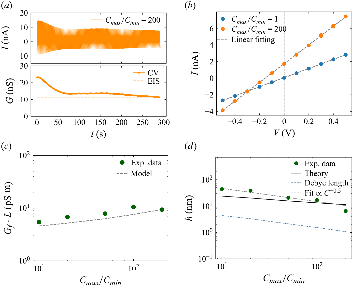
The electrical characterisation of the film nanochannel. (a) The CV measurements at a salt concentration ratio of 200 show time-dependent decay of nanochannel conductance magnitude (top). System conductance evolution from CV (solid curves) converges towards EIS baseline values (dashed) over time (bottom). (b) Typical I–V curves at the saturated states at salt concentration ratios of 1 (blue circles) and 200 (orange circles) show the Ohmic behaviour of the system. The dashed line represents a linear fit. (c) Nanochannel conductance per unit length across tested conditions (green circles), with theoretical predictions (black dashed line). (d) Normalised conductance-derived film thickness (green circles) versus salt concentration ratio at pH 9. The solid line shows the theoretical value of film thickness. The blue dashed line is the Debye length and the black dashed line shows the scaling law for the film thickness.

3. Experimental results
3.1. Ionic conduction
Typical results for the bubble film under a sweeping voltage are shown in figure 2(a, top), with 200 mM NaCl solution on the left and 1 mM NaCl solution on the right-hand side of the bubble. By linear fitting of the
 $I{-}V$
curves, we obtained the system conductance decreasing gradually over successive scanning cycles (figure 2
a, bottom), and finally reaching a saturated value. We could observe such a reduction in all of our electrical measurements for the beginning scanning cycles. We attribute the initial reduction and saturation of the bubble film conductance to the drainage of trapped water within the film. As the electro-osmotic flow induced by the scanning voltage drains this excess water trapped in the film, the film thins until it stabilises at a constant equilibrium thickness. This thickness is determined by the balance between capillary and disjoining pressures (Ma et al. Reference Ma, Sun, Duan, Van Den, Albert, Jan and Xie2020; Niu & Xie Reference Niu and Xie2025). The results show that the saturated conductance obtained by EIS is in agreement with that determined by cyclic voltammetry (CV) (figure 2
a, bottom).
We analysed the saturated conductance extracted from the
 $I{-}V$
curves (figure 2
b). Blue data points in figure 2(b) represent the results under symmetric (1 mM NaCl) concentration electrolyte solution filled on both sides, while the orange points were obtained under asymmetric concentration conditions with 1 mM NaCl filled in the right and 200 mM in the left reservoir. By linear fitting (dashed lines), we determined the film conductance in both conditions. A net current was found at
 $V = 0$
under a concentration gradient confirming a diffusion current across the bubble film, with the average value over the last ten consecutive cycles after the system reached a steady state.
To eliminate the variations of bubble length in each measurement, we evaluated the length-corrected conductance from the
 $I$
–
 $V$
slopes (figure 2
c). The corrected conductance (
 $G_{\!f} L$
, with
 $L$
denoting the bubble length) increased with the salt concentration ratio but decreased at the highest ratio, likely due to film thinning at high ionic strength.
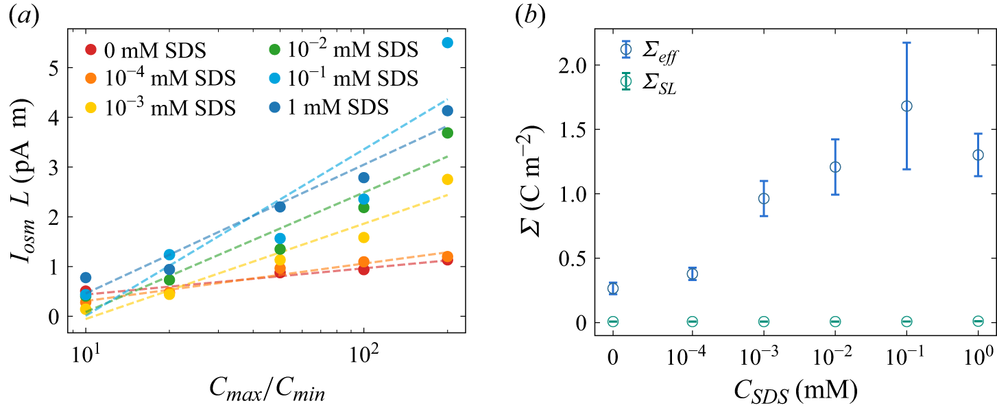
(a) Diffusion current per unit length at different SDS concentrations. (b) The effective charge density at the gas–solid–liquid interface (blue open circles) from diffusion current measurements at a salt concentration of 1 mM, and at the SL interface (green open circles) from electrokinetic current measurements.

Figure 3. Long description
Panel A: A line graph shows the diffusion current per unit length at different SDS concentrations. The x-axis represents the ratio of maximum to minimum concentration (Cmax/Cmin) on a logarithmic scale, while the y-axis represents the diffusion current per unit length (IosmL) in picoamperes per centimeter (pA cm). Different colored dots and dashed lines represent various SDS concentrations ranging from 0 mM to 1 mM. The graph indicates an increasing trend in diffusion current with higher SDS concentrations. Panel B: Another line graph displays the effective charge density at the gas-solid-liquid interface (blue open circles) and at the solid-liquid interface (green open circles). The x-axis represents the SDS concentration (CSDS) in millimolar (mM) on a logarithmic scale, and the y-axis represents the effective charge density (Σ) in coulombs per square meter (C m^-2). The blue open circles show an increasing trend in effective charge density with higher SDS concentrations, while the green open circles remain relatively constant.
3.2. Diffusion current measurement
Introducing a higher salt concentration on the left-hand side of the capillary than that on the right-hand side (1 mM NaCl) produced a net current at zero bias (
 $V = 0$
), driven by a chemical potential gradient across the bubble (Fair & Osterle Reference Fair and Osterle1971). This diffusion current reflects ion selectivity within the electric double layers (EDLs) at the LG and SL interfaces. Counterions dominate both the charge transport and the diffusio-osmotic flow within the bubble film.
We fixed the salt concentration in the right-hand reservoir (
 $C_{\textit{min}}=1$
mM) and varied the left-side concentration (
 $C_{\textit{max}}$
) from 10 to 200 mM to probe the effect of the salt gradient on diffusion current and conductance. Similar to the conductance, to account for variations in bubble length, we normalised the measured diffusion current by the film length (
 $I_{\textit{sys}} L$
), enabling consistent comparison across experiments. As shown in figure 3(a), the normalised diffusion current (red circles) increases linearly with
 $\mathrm{ln}(C_{\textit{max}}/C_{\textit{min}})$
.
Surfactants play a crucial role in determining the slip length at the LG interface and the zeta potential (Joly et al. Reference Joly, Detcheverry and Biance2014), significantly affecting electrokinetic phenomena, even at trace amounts (Peaudecerf et al. Reference Peaudecerf, Landel, Goldstein and Luzzatto-Fegiz2017; Landel et al. Reference Landel, Peaudecerf, Temprano-Coleto, Gibou, Goldstein and Luzzatto-Fegiz2020). Therefore, investigating the impact of surfactant concentration on zeta potential and slip boundaries via diffusion current is important. Here, we gradually changed the SDS concentration (
 $ C_{\textit{SDS}}$
) from 0 to 1 mM, while keeping the concentration gradient of NaCl solution across the bubble as a constant (
 $C=1 \,\mathrm{mM}$
). As shown in figure 3(a), the normalised diffusion current remains proportional to
 $\mathrm{ln}(C_{\textit{max}}/C_{\textit{min}})$
, in different slopes as
 $ C_{\textit{SDS}}$
varies. This change is likely due to the variation in surface charge density caused by the adsorption of ionic surfactants (SDS), which we analyse below.
4. Theoretical analysis
In this section, we analytically calculate the effective surface charge density and effective slip length at the LG interface. We first determine the film thickness from conduction which we found is larger than the Debye length, as shown in figure 2(d), which indicates the diffusion current can be calculated within the Debye length, instead of film thickness. Then, we derive an effective surface charge density of the liquid-film system (
 ${\varSigma }_{\textit{eff}}={\varSigma }_{\textit{LG}}^{\textit{eff}}+{\varSigma }_{\textit{SL}}$
) from the measured diffusion current, including the contribution from LG and SL interfaces. By streaming current measurements, we characterised the surface charge density at the SL interface
 ${\varSigma }_{\textit{SL}}$
. Therefore, we can derive the effective surface charge density at the LG interface
 ${\varSigma }_{\textit{LG}}^{\textit{eff}}$
by deduction of
 ${\varSigma }_{\textit{SL}}$
from the liquid-film system (§§ 2 and 3). Finally, we could estimate the slip length at the LG interface using the isotherm adsorption of surfactants, in various surfactant concentrations (§ 4).
4.1. Ionic conduction and film thickness
The effective film thickness
 $h$
is calculated from conduction measurements. Under a salt-concentration gradient, we treat the liquid resistance as series connection of infinitesimal resistors. Thus, the resistance can be expressed by
 \begin{equation} R_{\!f}=\frac {1}{G_{\!f}}={\int _0^L\frac {\text{d}x}{2\pi r h\left [k_b\!\left (C(x)\right )+k_s\!\left (C(x)\right )\right ]}} ,\end{equation}
where
 $r$
is the bubble radius of the glass capillary. Here, the thickness obtained from (4.1) is interpreted as an effective film thickness derived from the measured conductance, rather than a local thickness profile
 $h(x)$
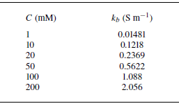
. The bulk conductivity of electrolytes solution (Appendix C, table 2) is a function of axis position
 $C(x)$
considering the salt gradient. To describe the axial salt transport in the film under finite advection, we consider the one-dimensional steady advection–diffusion equation with averaged velocity
 $u$
and diffusivity
 $D$
. The axial concentration field then satisfies the diffusion–convection equation (Lee et al. Reference Lee, Cottin-Bizonne, Biance, Joseph, Bocquet and Ybert2014a
)
 \begin{equation} D\frac {\text{d}^2C}{\text{d}x^2}-u\frac {\text{d}C}{\text{d}x}=0 .\end{equation}
With boundary condition of
 $C(0)=C_{\textit{max}}$
and
 $C(L)=C_{\textit{min}}$
, we obtain
 \begin{equation} C(x)=C_{\textit{max}}+(C_{\textit{min}}-C_{\textit{max}})\frac {\mathrm{exp}(\textit{Pe}\boldsymbol{\cdot }x/L)-1}{\mathrm{exp}(\textit{Pe})-1}, \end{equation}
where
 $\textit{Pe}=\textit{uL}/D$
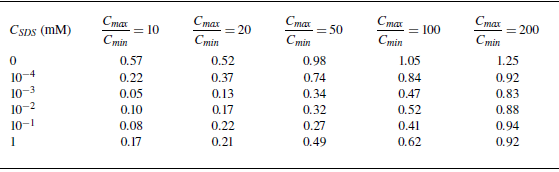
. The Péclet numbers in our experiments are listed in table 3 of Appendix C and range from
 $0.05$
to
 $1.25$
, where the maximum value occurs in the surfactant-free conditions at the largest salinity gradient. The concentration profile comes to the linear distribution when limit
 $\textit{Pe} \ll 1$
.
Considering the surface conductivity arising from the EDLs at both LG and SL interfaces, we have (Levine et al. Reference Levine, Marriott and Robinson1975)
 \begin{equation} k_s(C)=\frac {\mu \left (\mathit{\varSigma _{\textit{LG}}}(C)+\mathit{\varSigma _{\textit{SL}}}(C)\right )}{h}\left (1+\frac {e}{2\pi \ell _B\mu \eta }\right )\!, \end{equation}
where
 $\mu$
,
 $\ell _B$
,
 $e$
and
 $\eta$
are the counterion mobility, Bjerrum length, elementary charge and viscosity, respectively.
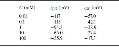
We fitted the zeta potential at various salt concentrations (see Appendix C, table 4) for surfactant-free LG interface (
 $\zeta _{\textit{LG}}$
) and SL interface (
 $\zeta _{\textit{SL}}$
) based on our previous experimental data (Ma et al. Reference Ma, Sun, Duan, Van Den, Albert, Jan and Xie2020), obtaining
 \begin{equation} \zeta _{\textit{LG}}(C)=4.34\,\ln (C-0.0019)-45.2 \quad \text{(mV)} ,\end{equation}
 \begin{equation} \zeta _{\textit{SL}}(C)=14.9\,\ln (C+0.420)-104 \quad \text{(mV)}. \end{equation}
We take the Grahame relation to connect the surface potential to surface charge densities, which are later used in the surface conduction term in (4.4). Here, the LG zeta potential
 $\zeta _{\textit{LG}}$
denotes the zeta potential at the LG interface that is used for film thickness calculation. The effective film thickness can be obtained by substituting the bulk conductivity and surface conductivity equation (4.4) into (4.1).
Given the measured
 $G_{\!f}$
, we solve (4.1) numerically and obtain a thickness
 $h$
across a broad range of salt concentrations (green circles in figure 2
d). The results show that the film thickness
 $h\propto C^{-0.5}$
(dashed line in figure 2
d), consistent with our previous studies (Ma et al. Reference Ma, Sun, Duan, Van Den, Albert, Jan and Xie2020).
The conductance-based film thickness obtained from (4.1)–(4.6) is shown as the circles in figure 2(d). We examine the film thickness by force balance between capillary pressure
 $p_c$
and disjoining pressure
 $\varPi _d$
under the salt-gradient conditions, for which theoretical film thickness changes with salt concentration. In a surfactant-free NaCl solution system, we use the DLVO description and consider the disjoining pressure
 $\varPi _d$
including the contribution from the van der Waals term
 $\varPi _{vdW}$
and the electrostatic term
 $\varPi _{el}$
. Since the salt concentration changes along the film axis, the electrostatic term was averaged along the axial direction of the film. The force balance
 $p_c =\varPi _d$
is therefore written as follows:
 \begin{equation} p_c =\varPi _{vdW}(h) + \frac {1}{L}\int _0^L \varPi _{el} \,\text{d}x. \end{equation}
Capillary pressure of the bubble meniscus is given by
 $p_c = 2{\mathit{\gamma } \cos \alpha }/{r}$
, where
 $\mathit{\gamma }$
and
 $\mathit{\alpha }$
are the interfacial tension and apparent wetting angle of the bubble, respectively. Here, we have approximated the curvature radius as the capillary radius
 $r$
, since the film thickness
 $h$
is negligible compared with the capillary radius. The apparent wetting angle of the bubble was optically measured in the capillary using image analysis software (drop shape analysis), yielding a value of
 $15^\circ$
. The van der Waals pressure is
 $\varPi _{vdW} = {-A}/{6\pi h^3}$
, where
 $A$
is the Hamaker constant for the fused silica–water–air system, reported as
 $A=-1.03 \times 10^{-20} \ \mathrm{J}$
(Hough & White Reference Hough and White1980). The electrostatic repulsion is
 $\varPi _{el}(C(x)) = 64k_BTn_{\infty }\mathit{\varGamma }_1(C(x))\mathit{\varGamma }_2(C(x)) \exp (-h/\lambda _D )$
(Ma et al. Reference Ma, Sun, Duan, Van Den, Albert, Jan and Xie2020), where
 $\mathit{\varGamma }_1$
and
 $\mathit{\varGamma }_2$
are the dimensionless surface potentials at the LG and SL interfaces. These surface potentials
 $\varGamma _i$
are related to the corresponding zeta potentials
 $\zeta _i$
by
 $\varGamma _i=\tanh ( {ze\zeta _i}/{4k_{\textit{B}}T} )$
, where
 $i=1,2$
. Here
 $z$
,
 $k_B$
,
 $T$
and
 $n_{\infty }$
are the ion valence, Boltzmann constant, temperature and bulk number density of the electrolyte ions, respectively, and
 $\lambda _D$
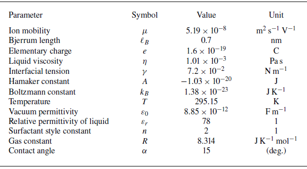
represents the Debye length. The physical constants used in the calculations are listed in table 1 of Appendix C.
Due to the force balance between Laplace pressure and disjoining pressure, we determine the theoretical film thickness numerically under the salt-gradient conditions (black solid line in figure 2
d). The corresponding Debye length, defined as the axial average of the local Debye length
 $\lambda _D$
, is shown by the dashed line in figure 2(d), where we have
 $h/\lambda _D\approx 3{-} 5.75$
in all probed concentrations, resulting in a thin EDL approximation. The surface potential drops to less than
 $5\,\%$
at the centre of the liquid film.
4.2. Diffusion current
The osmotic pressure drives the diffusion of counterions, as well as the diffusio-osmotic flow within the EDLs, generating an electric current, which has been known since the work of Fair & Osterle (Reference Fair and Osterle1971). The diffusion term can be written as
 $I_D = 2\pi r \int _{0}^{h} \text{d}z \, e (j_{D,+} - j_{D,-})$
, where
 $j_{D,\pm } = -D_s \boldsymbol{\nabla }C_{\pm }$
denotes the diffusive flux of cations/anions. For a symmetric electrolyte (assuming
 $D_+ \approx D_-=D_s$
), the net diffusion current across the channel can be approximated as
 $I_D=2\pi rD_s\partial _{x}{\varSigma }\approx 2\pi rD_s({\varSigma }(C_{\textit{max}})-{\varSigma }(C_{\textit{min}}))/L$
(Siria et al. Reference Siria, Poncharal, Biance, Fulcrand, Blase, Purcell and Bocquet2013). Since the surface charge density may be changed by the salt concentration (Najafi et al. Reference Najafi, Drelich, Yeung, Xu and Masliyah2007), here we estimate the diffusion term. Under the largest salt concentration gradient (200 mM−1 mM), we found that the diffusion term caused by surface charge density gradient has only
 $2\,\%$
contribution in the system, by taking
 ${\varSigma }(C_{\textit{max}} )=-0.0234 \ \mathrm{C\,m}^{-2}$
,
 ${\varSigma }(C_{\textit{min}} )=-0.0037 \ \mathrm{C\,m}^{-2}$
,
 $L=656\,{\unicode[Arial]{x03BC}} \mathrm{m}$
and
 $D_s=1.33\times 10^{-9}\ \mathrm{m^2\,s}^{-1}$
in the above calculation. Thus, the small contribution from the diffusion term arises from small surface charge density gradient, enabling us to make a constant charge density assumption along the axis of the liquid film for simplicity.
As a result, the measured diffusion current
 $I_{\textit{sys}}$
arises from the diffusio-osmotic flow which drives counterion diffusion within the EDL of both SL (
 $I_{\textit{SL}}$
) and LG (
 $I_{\textit{LG}}$
) interfaces. We define the diffusion current
 $I_i$
at either interface
 $i$
(SL or LG) as
 \begin{equation} I_{i} = 2\pi r \int _{\textit{film}} e (C_+ - C_-) u_i(z) \, \text{d}z .\end{equation}
To evaluate integral (4.8), we must derive the expression of flow velocity
 $u_i(z)$
at both LG and SL interfaces.
4.3. Diffusio-osmotic flow
Our liquid-film channel is considered as a two-dimensional slit system with a (upper) SL and (lower) LG interface, as shown in figure 2(b). The LG interface is treated as a Navier slip boundary with slip velocity
 $u_{\textit{slip}}=b(\partial u/\partial z) |_{z=0}$
, while the SL interface at the capillary wall is treated as a no-slip boundary (
 $u|_{z=h}= 0$
).
Moreover, even if a weak diffusio-osmotic convection exists, it still has a minor effect on the ion distribution compared with the EDL within the liquid film. In our experiments, the bubble length (
 $\sim$
1 mm scale) is much larger than the liquid film thickness (
 $h\sim 10$
nm range). Thus, the axial potential caused by external bias is much weaker than the transverse one caused by the EDL (
 $\partial ^2 \phi /\partial x^2 \ll \partial ^2 \phi /\partial z^2$
). Therefore, we still can approximate the counterion distribution by classical EDL theories, and the convection only provides a higher-order (minor) correction to the axial profile
 $C(x)$
(Prieve et al. Reference Prieve, Anderson, Ebel and Lowell1984):
 \begin{equation} C_\pm (x,z)=C_\infty (x)\exp(\mp \varPhi (z)), \end{equation}
where
 $C_+(x,z)$
and
 $C_-(x,z)$
denote the density of positive and negative ions near the charged surface, respectively, and
 $\varPhi ={e\phi }/{k_{\textit{B}}T}$
is the surface potential
 $\phi$
normalised by thermal energy
 $k_{\textit{B}}T$
.
The diffusio-osmotic velocity in the liquid film
 $\boldsymbol{u}$
is determined by the Stokes equation:
 \begin{equation} \eta \boldsymbol{\nabla} ^2 \boldsymbol{u} - \boldsymbol{\nabla }P + e (C_+ - C_-)(- \boldsymbol{\nabla }\psi )= 0, \end{equation}
where
 $ P$
is the pressures inside of the liquid film including the disjoining pressures between SL and LG interfaces as the normal vector and the osmotic pressure gradient across the bubble as the parallel factor. We may derive the pressure
 $ P$
by integrating the
 $z$
component of (4.10) using (4.9) for the ion distributions:
 \begin{equation} P(x, z) = P_\infty + 2k_{\textit{B}}T C_\infty (x) [\cosh (\varPhi (z)) - 1]. \end{equation}
Substituting (4.11) into the
 $x$
component of (4.10), the diffusio-osmotic velocity profile can be written as
 \begin{equation} \eta \frac {\text{d}^2 u}{\text{d}z^2} = 2k_{\textit{B}}T \left [ \cosh \varPhi (z) - 1 \right ] \frac {\text{d}C_\infty }{\text{d}x}. \end{equation}
In the liquid-film nanochannel, the microbubble surface is modelled as the LG interface, which defines the inner boundary of the film at
 $z=0$
, while the outer boundary at
 $z=h$
is the SL interface. We impose no-slip condition at the SL interface,
 $u(h)=0$
, and a Navier slip condition at the LG interface. We first consider the diffusion-driven flow with interfacial slip, for which the slip velocity obeys
 \begin{equation} u_{\textit{slip}}= b \frac {\partial u}{\partial z}\Big |_{z=0}, \end{equation}
where
 $b$
is the slip length and
 $u_{\textit{slip}}$
is the slip velocity at the LG interface, incorporating the influence of the Marangoni effect. By integrating (4.12) along the
 $z$
direction, and taking the boundary condition (4.13), we obtain the slip velocity at the LG interface under diffusio-osmosis:
 \begin{equation} u_{\textit{slip}} = -b \frac {2k_{\textit{B}}T}{\eta } \left [ \int _0^{h/2} \left [ \cosh \varPhi (z) - 1 \right ]\, \text{d}z \right ] \frac {\text{d}C_\infty }{\text{d}x}. \end{equation}
Using the thin EDL approximation, the integral can be evaluated analytically to leading order. Using the identity
 $\text{d}z = -\text{d}\varPhi /(\kappa \sqrt {2(\cosh \varPhi -1)})$
derived from the Poisson–Boltzmann equation, the integral term becomes (Mouterde & Bocquet Reference Mouterde and Bocquet2018)
 \begin{equation} \int _{0}^{h/2} (\cosh \varPhi - 1) \text{d}z = \frac {2}{\kappa }\left(\sqrt {1+(1/\kappa \ell _{\textit{GC}})^2}-1\right)\!. \end{equation}
Here,
 $\ell _{\textit{GC}} = (2\pi \ell _B \varSigma _n)^{-1}$
is the Gouy–Chapman length and
 $\kappa = \sqrt {8\pi \ell _B C_{\infty }}$
is the inverse Debye length.
To make the gradient term dimensionless, we use
 $\kappa ^2 = 8\pi \ell _B C_{\infty }$
:
 \begin{equation} \frac {\text{d}C_{\infty }}{\text{d}x} = C_{\infty } \frac {{\rm d} \ln C_{\infty }}{\text{d}x} = \frac {\kappa ^2(C_\infty )}{8\pi \ell _B} \boldsymbol{\nabla} _x \ln C_{\infty }. \end{equation}
Substituting the integral result (4.15) and this gradient transformation back into (4.14) yields the final expression for the diffusio-osmotic slip velocity:
 \begin{equation} u_{\textit{slip}} = \frac {k_{\textit{B}}T}{2\pi \eta \ell _B} \frac {b}{\lambda _D} \left [ \sqrt {1 + \left ( \frac {1}{\kappa \ell _{\textit{GC}}} \right )^2} - 1 \right ] (-\boldsymbol{\nabla} _x \ln C_{\infty }). \end{equation}
4.4. Current–slip relationship
Using the diffusio-osmotic velocity profile
 $u(z)$
derived in § 4.3, we now obtain the analytical expression for the diffusion current at the liquid film. The current results from the advection of the net charge density (
 $\rho _e = e(C_+ - C_-)$
) within the EDL. By integrating the product of charge density and flow velocity across the film thickness, we directly relate the macroscopic measurable current to the microscopic slip length.
According to (4.8), we have obtained the diffusion current
 $I_{\textit{LG}}$
at the LG interface as
 \begin{equation} I_{\textit{LG}} = 2\pi r \int _0^{h/2} e (C_+ - C_-) u(z) \, \text{d}z. \end{equation}
Using the Poisson equation
 $ C_+ - C_- = -{(\text{d}^2\varPhi /\text{d}z^2) }/{4\pi \ell _B}$
(Andelman Reference Andelman1995), the diffusion current (4.8) can be written as
 \begin{equation} I_{\textit{LG}} = 2\pi r \frac {e}{4\pi \ell _B} \int _0^{h/2} \left (-\frac {\text{d}^2\varPhi }{\text{d}z^2} \right ) u(z) \, \text{d}z. \end{equation}
We then integrate (4.19) twice along the zdirection and obtain
 \begin{align} I_{\textit{LG}} = \frac { e r }{2\ell _B} \left \{ \frac {\text{d}\varPhi }{\text{d}z}(0) u(0) - \varPhi (0) \frac {\text{d}u}{\text{d}z}(0) - \int _0^{h/2} \varPhi (z) \left [ \cosh \varPhi (z) - 1 \right ]\, \text{d}z \times \frac {2k_{\textit{B}}T}{\eta } \frac {\text{d}C_\infty }{\text{d}x} \right \}\!, \end{align}
where
 $u(0)=u_{\textit{slip}}$
is the slip velocity at the LG interface given by (4.17). In a thin-Debye-length limit, we have
 $\text{d}z = - {\text{d}\varPhi }/({\kappa \sqrt {2[\cosh \varPhi (z)-1]}})$
according to Mouterde & Bocquet (Reference Mouterde and Bocquet2018).
From (4.12), the Stokes equation is also used to calculate the shear rate at the LG surface:
 \begin{equation} \frac {\text{d}u}{\text{d}z}(z = 0) = - \frac {2k_{\textit{B}}T}{\eta } \int _0^{h/2} \left [ \cosh \varPhi (z) - 1 \right ]\, \text{d}z \times \frac {\text{d}C_\infty }{\text{d}x}. \end{equation}
Combining the slip velocity (4.17) and the relation
 ${\varSigma }_{\textit{LG}}={-e{\varSigma }}_n$
, we derive the diffusion current. To rigorously justify the relative gradient term in (4.23), we apply the dimensional transformation established in (4.16):
 \begin{equation} \frac {\text{d}C_{\infty }}{\text{d}x} = \frac {\kappa ^2(C_\infty )}{8\pi \ell _B} \boldsymbol{\nabla} _x \ln C_{\infty }. \end{equation}
Substituting this relation into the integrated current expression effectively normalises the osmotic driving force by the local electrostatic length scales. Consequently, the final expression for the diffusion current is obtained as
 \begin{align} I_{\textit{LG}} = 2\pi r (- {\varSigma }_{\textit{LG}}) \frac {k_{\textit{B}}T}{2\pi \eta \ell _B} \! \left [ \frac {b}{\lambda _D} \! \left ( \sqrt {1 + \left ( \frac {1}{\kappa \ell _{\textit{GC}}} \right )^2} - 1 \right ) + \left(1-\kappa \ell _{\textit{GC}}\sinh ^{-1}\frac {1}{\kappa \ell _{\textit{GC}}}\right) \right ](- \boldsymbol{\nabla} _x \ln C_\infty ). \end{align}
In our experiments,
 $\ell _{\textit{GC}} \ll \lambda _D$
and the second term in (4.23) can be neglected. The axial salt concentration is described by the steady one-dimensional advection–diffusion profile introduced above. Integrating the logarithmic driving term along the film axis gives
 $\int _0^L -\boldsymbol{\nabla} _x \ln C_\infty (x)\, \text{d}x = \Delta \ln C_\infty$
, where
 $\Delta \ln C_\infty =\ln (C_{\textit{max}}/C_{\textit{min}})$
. The corresponding average logarithmic gradient is therefore
 $\Delta \ln C_\infty /L$
. The diffusion current at the LG interface can therefore be written in the reduced form
 \begin{equation} I_{\textit{LG}} \approx \frac {2\pi r (- {\varSigma }_{\textit{LG}})}{L} \frac {k_{\textit{B}}T}{2\pi \eta \ell _B} \left [ \frac {b}{\lambda _D} \left ( \sqrt {1 + \left ( \frac {1}{\kappa \ell _{\text{GC}}} \right )^2} - 1 \right ) + 1 \right ] \Delta\!\ln (C_\infty ). \end{equation}
For the SL interface, we take no-slip boundary conditions, and their contribution to the diffusion current becomes (Siria et al. Reference Siria, Poncharal, Biance, Fulcrand, Blase, Purcell and Bocquet2013)
 \begin{equation} I_{\textit{SL}} \approx \frac {2\pi r{(-{\varSigma }}_{\textit{SL}})}{L}\frac {k_BT}{2\pi \eta \ell _B}\Delta \ln {\left (C_\infty \right )}, \end{equation}
where
 ${\varSigma }_{\textit{SL}}$
is the surface charge density of the SL interface.
Therefore, the diffusion current in the liquid film considering the LG interface (
 $I_{\textit{LG}}$
) and SL interface (
 $I_{\textit{SL}}$
) of the bubble becomes
 \begin{equation} I_{\textit{sys}}=-\frac {2\pi r}{L}\frac {k_BT}{2\pi \eta \ell _B} {\varSigma }_{\textit{eff}} \Delta \ln (C_\infty ), \end{equation}
where
 ${\varSigma }_{\textit{eff}}$
is the effective surface charge density considering the diffusion current contributed from the LG and SL interfaces.
Here we introduce an effective surface charge density of the system, considering the non-slip SL and slipping LG interfaces:
 \begin{equation} {\varSigma }_{\textit{eff}}={\varSigma }_{\textit{SL}}+{\varSigma }_{\textit{LG}}\left [\frac {b}{\lambda _D}\left (\sqrt {1+\left(\frac {1}{\kappa \ell _{\textit{GC}}} \right)^2}-1\right )+1\right ]\!. \end{equation}
As seen from (4.27), the effective surface potential (or surface charge density) can be enhanced with a boundary slip.
4.5. Slip length
To decouple the contributions of the two interfaces, we first recognise that the surface charge density at the SL interface
 ${\varSigma }_{\textit{SL}}$
is associated with a no-slip boundary, and therefore independent of the slip length. This value is measured independently via streaming current experiments (see Appendix A). By subtracting this known
 ${\varSigma }_{\textit{SL}}$
from the total system charge
 ${\varSigma }_{\textit{eff}}$
(4.27), we isolate the effective surface charge density at the LG interface, which explicitly relates to the slip length
 $b$
as
 \begin{equation} \mathit{{\varSigma }}_{\textit{LG}}^{\textit{eff}}=\mathit{{\varSigma }}_{\textit{LG}}\left [\frac {b}{\lambda _D}\left (\sqrt {1+{\left(\frac {1}{\kappa \ell _{\textit{GC}}}\right)}^2}-1\right )+1\right ]\!. \end{equation}
To estimate
 $\varSigma _{\textit{LG}}$
, we consider the surfactant adsorption dynamics at the LG interface. The adsorption of SDS is typically described by the Frumkin isotherm, which accounts for lateral interactions between adsorbed molecules (Prosser & Franses Reference Prosser and Franses2001). However, given the low surfactant concentration in our experiments (
 $C_{\textit{SDS}}\leqslant 1$
mM), the system operates in the dilute regime, where the Frumkin isotherm simplifies to the linear Henry adsorption isotherm (Sundin & Bagheri Reference Sundin and Bagheri2022):
 \begin{equation} S=k_d{\mathit{\varGamma }}_\infty \left(C_k \frac {C_{\textit{sur}}}{C_{\textit{SDS}}}- \frac {\mathit{\varGamma }}{{\mathit{\varGamma }}_\infty }\right)\!, \end{equation}
where
 $S$
is the adsorption–desorption flux of surfactants at the LG interface. Parameters
 $C_{\textit{sur}}$
and
 $\mathrm{\mathit{\varGamma }}$
are the bulk surfactant concentration within the liquid film and the surface surfactant concentration adsorbed at the LG interface.
The dimensionless bulk surfactant concentration
 $C_k=k_a C_{\textit{SDS}}/k_d$
indicates the surfactant concentration at the LG interface under the adsorption–desorption equilibrium, where
 $k_a$
is the adsorption coefficient and
 $k_d$
is the desorption coefficient. Based on the experimental parameters compiled by Prosser & Franses (Reference Prosser and Franses2001), we adopt the low-salinity limit values to approximate our 1 mM NaCl background. Specifically, we use
 $k_a/k_d=0.179\,\mathrm{m^3\, mol^{-1}}$
and the maximum concentration of SDS adsorbed at the LG interface is
 $\mathrm{\mathit{\varGamma }}_\infty =1/(2.551\times {10}^5)$
 $\mathrm{mol} \,\mathrm{m}^{-2}$
. In this dilute regime, the fraction of bound counterions is negligible (Joly et al. Reference Joly, Detcheverry and Biance2014), allowing us to assume that the adsorbed surfactant monolayer is fully dissociated.
At equilibrium state, where the amount of surfactant adsorbed and desorbed at the LG surface is balanced (
 $S \approx 0$
), the surfactant concentration within the liquid film equals the bulk surfactant concentration in electrolyte solution (
 $C_{\textit{sur}} \approx C_{\textit{SDS}}$
). Substituting
 $S=0$
and
 $C_{\textit{sur}} \approx C_{\textit{SDS}}$
into (4.29) yields the surface surfactant concentration at the LG interface,
 $\mathrm{\mathit{\varGamma }}=k_a\mathrm{\mathit{\varGamma }}_\infty C_{\textit{SDS}}/k_d$
. Thus, the surface charge density at the LG interface
 ${\varSigma }_{\textit{LG}}$
becomes
 \begin{equation} \mathrm{{\varSigma }}_{\textit{LG}}=\frac {{eN_Ak}_a\mathrm{\mathit{\varGamma }}_\infty C_{\textit{SDS}}}{k_d}+\mathrm{{\varSigma }}_{0}, \end{equation}
where
 $N_A$
is the Avogadro constant and
 ${\varSigma }_{0}=0.003716$
 $\mathrm{C}\, \mathrm{m}^{-2}$
is the surface charge density of the pure LG interface (Ma et al. Reference Ma, Sun, Duan, Van Den, Albert, Jan and Xie2020). Using (4.28), the slip length
 $b$
can be expressed as
 \begin{equation} b=\frac {\lambda _D({\varSigma }_{\textit{LG}}^{\textit{eff}}/{\varSigma }_{\textit{LG}}-1)}{\sqrt {1+( {1}/{\kappa \ell _{\textit{GC}}})^2}-1}. \end{equation}
Equation (4.31) quantitatively describes the relationship between slip length and surface charge density, enabling us to characterise the hydrodynamic slip via enhanced surface potential and electrokinetic phenomena.
5. Experimental results
5.1. Derivation of effective surface charge density
According to (4.26), the normalised diffusion current
 $I_{\textit{sys}}L$
is proportional to the osmotic pressure (
 $\sim RT\ln (C_{\textit{max}}/C_{\textit{min}})$
) in various SDS concentrations, as observed in figure 3(a). The addition of SDS surfactant significantly enhances the diffusion current within the bubble liquid film when
 $C_{\textit{SDS}} \leqslant 1$
mM, which we attributed to the joint actions of adsorbed surfactants and the slip length at the LG interface.
To quantify these effects, we determine the effective surface charge density of the liquid film system,
 ${\varSigma }_{\textit{eff}}$
, which includes contributions from both LG and SL interfaces. Following (4.26),
 ${\varSigma }_{\textit{eff}}$
is extracted from the slopes of the linear fits in figure 3(a). The results are shown as blue circles in figure 3(b), with error bars given by the standard deviation of the linear fitting. The effective surface charge density
 ${\varSigma }_{\textit{eff}}$
varies non-monotonically with surfactant concentration. Here
 ${\varSigma }_{\textit{eff}}$
increases with
 $C_{\textit{SDS}}$
, reaches a maximum near
 $C_{\textit{SDS}} \approx 10^{-1}$
mM and then decreases at higher concentrations.
To separate the contribution from the SL interface, we performed streaming current measurements (Delgado et al. Reference Delgado, González-Caballero, Hunter, Koopal and Lyklema2007) in a glass capillary without a bubble using 1 mM NaCl solutions at different SDS concentrations (Appendix A). The derived
 ${\varSigma }_{\textit{SL}}$
values (green circles) remain nearly constant at all surfactant concentrations, as shown in figure 3(b). The constant zeta potential at the SL surface could be understood as the intrinsic surface charge density of the glass surface (pH = 9), while adsorption of SDS has a limited contribution.
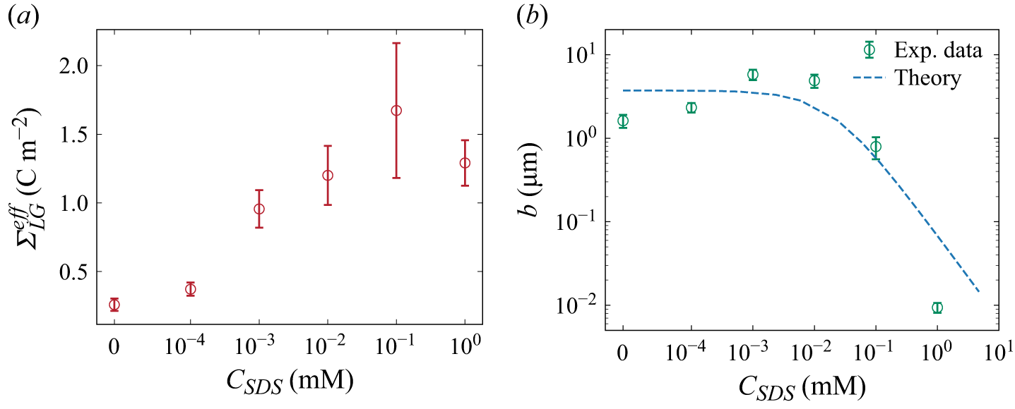
(a) Measured the effective surface charge density
 ${\varSigma }_{\textit{LG}}^{\textit{eff}}$
(red circles) versus SDS concentration
 $C_{\textit{SDS}}$
at 1 mM NaCl. (b) Interfacial slip length as a function of
 $C_{\textit{SDS}}$
, demonstrating suppression at
 $C_{\textit{SDS}} \geqslant 10^{-2}$
mM due to interfacial immobilisation.

With the characterised
 ${\varSigma }_{\textit{SL}}$
, we can derive an effective surface charge density at the LG interface
 ${\varSigma }_{\textit{LG}}^{\textit{eff}}$
from (4.27). The resulting
 ${\varSigma }_{\textit{LG}}^{\textit{eff}}$
(red circles in figure 4
a) is much larger than
 ${\varSigma }_{\textit{SL}}$
, due to the joint action of adsorbed ionic surfactants and boundary slip. Equation (4.28) describes the amplifications by hydrodynamic slip by a factor of
 $b/\lambda _D$
.
As
 $C_{\textit{SDS}}$
increases, we found that
 ${\varSigma }_{\textit{LG}}^{\textit{eff}}$
initially rises, consistent with the quantity of anionic surfactants adsorbed at the LG interface. When
 $C_{\textit{SDS}}\gt 10^{-1}$
mM,
 ${\varSigma }_{\textit{LG}}^{\textit{eff}}$
begins to plateau and eventually decreases. We attribute this non-monotonic trend to a reduction in slip length caused by surfactant adsorption at the LG interface. At sufficiently high SDS concentrations, the adsorbed layer becomes less mobile and increases interfacial friction, which suppresses slip and weakens the slip-amplification effect. At
 $C_{\textit{SDS}}=1$
mM, the slip length is strongly reduced, approaching a no-slip limit, and
 ${\varSigma }_{\textit{LG}}^{\textit{eff}}$
decreases despite the higher surfactant coverage.
5.2. Derivation of slip length at the LG interface
With the isolated zeta potential at the LG interface, we could derive the intrinsic slip length at the LG interface as a function of surfactant concentration by using (4.31). The green circles in figure 4(b) represent the derived slip length from the measured zeta potential, and the dashed lines are the theoretical predictions that were developed in this work based on our previous theoretical framework (Yan et al. Reference Yan, Niu, Sun and Xie2025) as shown in Appendix B.
When the surfactant concentration is lower than
 $10^{-2}$
mM, the slip length remains nearly constant, approaching 3
 ${\unicode[Arial]{x03BC}} \mathrm{m}$
as the intrinsic slip length at the LG interface. Our results indicate that a small amount of SDS surfactant will not clearly reduce the slip length, which is in agreement with theoretical predictions (Peaudecerf et al. Reference Peaudecerf, Landel, Goldstein and Luzzatto-Fegiz2017; Landel et al. Reference Landel, Peaudecerf, Temprano-Coleto, Gibou, Goldstein and Luzzatto-Fegiz2020; Yan et al. Reference Yan, Niu, Sun and Xie2025). However, when the surfactant concentration exceeds
 $10^{-2}$
mM, the slip length rapidly decreases, dropping by nearly two orders of magnitude at 1 mM. This dramatic reduction of slip length explains the decrease of zeta potential when surfactant concentration exceeds
 $10^{-1}$
mM in figure 4(a).
Based on the theoretical model, the reduction in slip length can be attributed to the joint actions of surfactant adsorption and Marangoni stresses. At low surfactant concentrations (
 $C_{\textit{SDS}} \lt 10^{-2}$
mM), adsorption–desorption processes at the LG interface are relatively balanced, resulting in small interfacial concentration gradients and negligible Marangoni stresses. Under such conditions, the slip length is governed primarily by the intrinsic interfacial friction of a clean surface. In contrast, at higher concentrations (
 $C_{\textit{SDS}} \gt 10^{-2}$
mM), surfactant adsorption increases markedly, amplifying the interfacial concentration gradient and enhancing Marangoni stresses. The associated rise in interfacial stress significantly reduces the slip length, which approaches a no-slip condition when
 $C_{\textit{SDS}}$
exceeds 1 mM. Thus, we could conclude that the zeta potential at surfactant-covered bubble film increases when
 $C_{\textit{SDS}} \lt 10^{-1}$
mM since the adsorbed SDS increases the charge density at the LG interface. However, the highly packed SDS molecules result in a significant increase of the friction coefficient at the LG interface, thus suppressing the slip length and zeta potential, as evident from both experimental and theoretical results.
The strongly enhanced effective surface charge density may significantly increase the electrokinetic phenomena and performance of potential applications like osmotic energy harvesting (Xu et al. Reference Xu, Yan and Xie2024). We gained electricity via net diffusion current across the bubble under osmotic pressure. The osmotic power is proportional to the square of effective surface charge density of nanochannels
 $P_{\textit{max}}=I_{\textit{sys}}^2/4G_{\!f} \propto {\varSigma }_{\textit{eff}}^2$
(Ren & Stein Reference Ren and Stein2008; Siria et al. Reference Siria, Poncharal, Biance, Fulcrand, Blase, Purcell and Bocquet2013).
In conventional solid nanochannels, the surface potential is typically of the order of tens of millivolts under no-slip boundary conditions. However, owing to interfacial slip at the LG interface, the zeta potential may be significantly enhanced to
 $\sim 100$
mV range, due to the adsorption of ionic surfactant and boundary slip. Thus, the figure of merit in osmotic energy conversion can be enhanced by an order of magnitude, while the power generation was enhanced by 2–3 orders of magnitude.
However, since the non-conductive gas bubble occupies most of the area of the microchannel, the power density is strongly limited. But, if it is possible to work with foams or bubble lattices, which have a large surface-to-volume ratio of LG interface, it will be helpful to enhance the power density. Overall, the liquid-film nanochannel framework provides a route to use soft, slipping interfaces to enhance mass transport at the nanoscale.
6. Conclusion
In this work, we investigated the diffusion current, a family of electrokinetic phenomena, across a bubble interface, where a thin liquid film forms at the interface between a gas bubble and a cylindrical glass capillary. We first measured the diffusion current and film conductance, from which the film thickness was determined. Our results showed that the diffusion current increases with the osmotic pressure, allowing us to derive an effective zeta potential of the bubble film system. The presence of surfactants strongly increases the diffusion current and effective surface charge density at the LG interface, due to the enhanced surface charge density by ionic-surfactant adsorption at the LG interface, and reaches a peak value at
 $10^{-1}$
mM. However, the effective surface charge density starts to decrease once the surfactant concentration exceeds a threshold value, which we attribute to a reduction in the slip length.
To explain this behaviour, we formulated an analytical theory based on isotherm adsorption and Marangoni stress of adsorbed surfactants, to describe the surfactant-induced change of slip length at the LG interface. Our theory can well describe the diffusion current with a slip boundary under osmotic pressure, which helps to derive the slip length at the LG interface as a function of surfactant concentration. Our calculation from experimental results showed that the slip length at the LG interface remains nearly constant (3
 ${\unicode[Arial]{x03BC}} \mathrm{m}$
) when SDS concentration is below
 $10^{-2}$
mM. However, it dramatically decreases when
 $C_{\textit{SDS}}$
exceeds
 $10^{-2}$
mM due to the joint actions of increased surfactant adsorption and Marangoni stress. Both effects increase the friction of LG interfaces, decreasing the slip length at 1 mM SDS and approaching a no-slip condition. We demonstrate that boundary slip at the LG interface can reinforce osmotic power harvesting compared with no-slip systems. Our findings provide new insights into the electrokinetic and transport behaviour at solid–liquid–gas interfaces, offering a quantitative framework for understanding mass transport and interfacial slip under electric field effects.
Funding
This work is supported by the National Natural Science Foundation of China under grant nos. 12388101 and 12550001 and the Innovation Capability Support Program of Shaanxi under grant no. 2024RS-CXTD-15.
Declaration of interests
The authors report no conflict of interest.
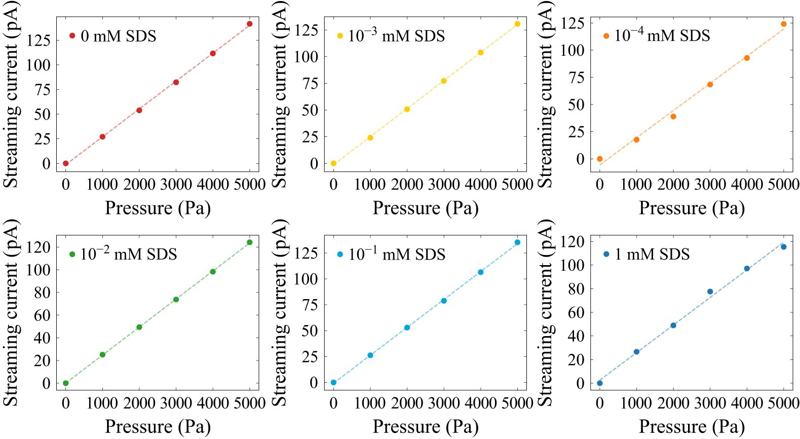
Appendix A. Zeta potential at the solid–liquid interface
We determine the zeta potential at the SL interface by measuring the streaming current in a glass capillary. When an external pressure difference
 $\Delta p$
is applied across the capillary, it induces fluid flow, which mobilises counterions in the EDL, generating a streaming current
 $I_{\textit{str}}$
. This current is related to the zeta potential
 $\zeta _{\textit{SL}}$
by the expression
 \begin{equation} I_{\textit{str}}=-\frac {\varepsilon _0\varepsilon _r\pi r_{c}^2}{\eta } \frac {\Delta p} {L_{c}} \zeta _{\textit{SL}}, \end{equation}
where
 $r_{c}=50$
 ${\unicode[Arial]{x03BC}} \mathrm{m}$
is the capillary radius and
 $L_c=1.5$
 $\mathrm{cm}$
is the capillary length.
To investigate the effect of surfactants, we use a Fluigent pressure pump to drive a 1 mM NaCl solution through the capillary while maintaining a fixed pH of 9. Ag/AgCl electrodes at both ends of the capillary, connected to a Keithley 6430 source meter, continuously record the streaming current. The SDS concentration is systematically varied from 0 to 1 mM while keeping the NaCl concentration constant at 1 mM. Figure 5 shows a linear relationship between streaming current and applied pressure difference for different SDS concentrations. By fitting the data to (A1), we extract the zeta potential
 $\zeta _{\textit{SL}}$
at the SL interface as a function of surfactant concentration. Based on the Gouy–Chapman theory, the corresponding surface charge density at the SL interface was calculated using the Grahame relation (Baldessari Reference Baldessari2008):
 \begin{equation} {\varSigma }_{\textit{SL}} = \frac {2\pi \ell _B\lambda _D}{e} \sinh \left (\frac {e\zeta _{\textit{SL}}}{2k_BT}\right )\!. \end{equation}
The streaming current exhibits a linear increase with the external pressure difference across a range of SDS concentrations.

Figure 5. Long description
The image contains six line graphs, each showing the relationship between streaming current (pA) and pressure (Pa) at different SDS concentrations. Panel A: The graph shows a red line representing 0 mM SDS. The streaming current increases linearly from 0 to 125 pA as the pressure increases from 0 to 5000 Pa. Panel B: The graph shows a yellow line representing 10^-3 mM SDS. The streaming current increases linearly from 0 to 125 pA as the pressure increases from 0 to 5000 Pa. Panel C: The graph shows an orange line representing 10^-4 mM SDS. The streaming current increases linearly from 0 to 125 pA as the pressure increases from 0 to 5000 Pa. Panel D: The graph shows a green line representing 10^-2 mM SDS. The streaming current increases linearly from 0 to 120 pA as the pressure increases from 0 to 5000 Pa. Panel E: The graph shows a blue line representing 10^-1 mM SDS. The streaming current increases linearly from 0 to 125 pA as the pressure increases from 0 to 5000 Pa. Panel F: The graph shows a dark blue line representing 1 mM SDS. The streaming current increases linearly from 0 to 120 pA as the pressure increases from 0 to 5000 Pa.
Appendix B. Slip length
To evaluate the boundary slip at the LG interface, we first calculate the friction coefficient of surfactants adsorbed at the interface. A single negatively charged surfactant molecule at the LG interface experiences friction due to the shear stress of surrounding water (first term in (B1)) and Marangoni effects (second term in (B1)). At steady state, the force on a single surfactant is balanced as
 \begin{equation} \lambda _{s}\left ( {u_{\textit{slip}} - u_{i}} \right ) - \frac {1}{N_{A}}\frac {{\textrm {d}} \mu }{{\textrm {d}} \textit {x}} = 0. \end{equation}
Here,
 $\lambda _s=3 \pi \eta r_d$
represents the friction coefficient between surfactants and the surrounding liquid (Joly et al. Reference Joly, Detcheverry and Biance2014), where
 $r_d$
denotes the hydration radius of the surfactant hydrophilic head. Parameter
 $u_i$
is the velocity of a single surfactant adsorbed at the LG interface. The term
 $\mathrm{d}\mu /{\mathrm{d}x}$
indicates the chemical potential gradient induced by non-uniform surfactant distribution. Consequently, solving (B1) gives the surfactant velocity:
 \begin{equation} u_{i} = u_{\textit{slip}} - \frac {1}{\lambda _{s}N_{A}}\frac {\mathrm{d}\mu }{\mathrm{d}x}. \end{equation}
To obtain a modified slip boundary condition in the presence of Marangoni stress, we consider the force balance on the interfacial fluid layer, consisting of the liquid and surfactants adsorbed at the LG interface as follows:
 \begin{equation} \left . {\eta \frac {{\textrm {d}} \textit {U}}{{\textrm {d}} \textit {z}}} \right |_{z = 0} -\lambda _s \varGamma\!N_A(u_{\textit{slip}}-u_i)-\lambda _0 u_{\textit{slip}} = 0. \end{equation}
Here,
 $U$
is the flow velocity within the liquid film,
 $\lambda _0$
is the friction coefficient between the liquid and a clean LG interface and
 $\varGamma$
is the surface surfactant concentration at the LG interface.
We next model the transport of surfactants along the LG interface. Surfactant accumulation downstream and depletion upstream lead to a surface tension gradient, which drives Marangoni stress. Since the liquid film thickness
 $h$
is far smaller than the bubble length
 $L$
, we derive a one-dimensional convection–diffusion equation for surfactants at the LG interface as
 \begin{equation} \frac {\partial \left ( {u_{i}\varGamma } \right )}{\partial x} = D\frac {\partial ^{2}\varGamma }{\partial x^{2}} + S, \end{equation}
where
 $D = 7.0 \times 10^{- 10}\,{\rm m}^{2}\,{\rm s}^{- 1}$
represents the diffusion coefficient of SDS surfactants, based on Peaudecerf et al. (Reference Peaudecerf, Landel, Goldstein and Luzzatto-Fegiz2017) and
 $S$
is the source term, indicating adsorption and desorption fluxes of surfactants at the LG interface.
The normal diffusive flux from the bulk to the interface is balanced by
 $S$
as follows:
 \begin{equation} D\frac {\partial c}{\partial z}|_{z = 0} = S. \end{equation}
Assuming a linear variation in surfactant concentration along the interface and uniform distribution at the bubble meniscus, we simplify the Frumkin adsorption isotherm to the Henry isotherm (Landel et al. Reference Landel, Peaudecerf, Temprano-Coleto, Gibou, Goldstein and Luzzatto-Fegiz2020), leading to a linearised form of
 $S$
:
 \begin{equation} S = k_{d}\varGamma _{\infty }\left ( {C_{k}{C_{\textit{sur}}}/{C_{\textit{SDS}}} - \theta } \right ), \end{equation}
where
 $C_k=k_aC_{\textit{SDS}}/k_d$
is the dimensionless bulk surfactant concentration,
 $C_{\textit{sur}}$
is the bulk surfactant concentration near the LG interface and
 $\theta =\varGamma /\varGamma _\infty$
is the dimensionless surface surfactant concentration at the LG interface, representing surfactant coverage. Utilising the linearised source term
 $S$
, we approximate
 $\theta =C_k$
at
 $x=0$
.
According to (B4)–(B6), and referring to the derivation process of Yan et al. (Reference Yan, Niu, Sun and Xie2025), we can obtain the surfactant reduction upstream of the bubble
 $\Delta \theta$
:
 \begin{equation} \Delta \theta = \frac {u_{\textit{slip}} C_k}{\frac {2D}{L} + \frac {L k_d}{4(1+k_a\varGamma _{\infty }h/D)}+ \frac {2\textit{nRT}}{N_A L \lambda _s}}. \end{equation}
The linearised Marangoni stress
 $f_M$
is related to this depletion
 $\Delta \theta$
as
 \begin{equation} f_M=-\textit{nRT}\varGamma _{\infty }\frac {2\Delta \theta }{L}, \end{equation}
where
 $n$
is the surfactant style constant.
From (B7) and (B8), the chemical potential gradient
 $\text{d}\mu /\text{d}x$
is expressed as
 \begin{equation} \frac {\text{d}\mu }{\text{d}x}=-\frac {f_M}{C_k \varGamma _{\infty }}=\frac {\alpha _s u_{\textit{slip}}}{C_k \varGamma _{\infty }}, \end{equation}
where the parameter
 $\alpha _s = {2\textit{nRT} \varGamma _ \infty C_k}/({2D+( {L^2 k_d}/({4(1+k_a\varGamma _{\infty }h/D)}))+ {2\textit{nRT}}/{N_A \lambda _s}})$
quantifies the strength of the Marangoni effect.
To estimate the slip length at the surfactant-covered LG interface, we derived the friction coefficient, given by
 $f=\lambda (u_{\textit{slip}} -u_i)$
. Here,
 $f$
is the stress borne by surfactants at the LG interface, which is equal to the negative value of the Newtonian shear stress, and
 $\lambda$
is the effective friction coefficient between liquid and gas considering viscous stress, electrostatic force and the Marangoni stress. Therefore, using (B1) and (B3), the total friction coefficient becomes
 \begin{equation} \lambda =\lambda _s\varGamma N_A+\frac {\lambda _0 \lambda _s N_A \varGamma _{\infty } C_k}{\alpha _s}. \end{equation}
The slip length can be derived by the Navier boundary condition
 $b=\eta /\lambda$
as
 \begin{equation} b=\frac {2\textit{nRT}\eta }{2nRT\lambda _s \varGamma _\infty N_A C_k+\lambda _0\lambda _sN_A \left[2D+\frac {L^2k_d}{4(1+k_a \varGamma _\infty h/D)}+\frac {2\textit{nRT}}{N_A \lambda _s}\right]} .\end{equation}
Equation (B11) shows that the slip length
 $b$
depends on the surfactant concentration. It can be observed that the slip length
 $b$
is related to the surfactant concentration. As the surfactant concentration approaches zero, the slip length tends towards a constant value corresponding to the clean interface. With increasing surfactant concentration, the slip length decreases and exhibits an inverse relationship, highlighting the dominant role of Marangoni-induced resistance.
Appendix C. Variables
Physical constants.

Table 1. Long description
A table listing physical constants with their symbols, values, and units. The table has 12 rows and 3 columns. The columns are labeled C (m M), ζ_LG (m V), and ζ_SL (m V). The rows list the following values: Row 1: 0.01, -117, -57.0. Row 2: 0.1, -115, -42.1. Row 3: 1, -94.3, -28.9. Row 4: 10, -65.0, -27.4. Row 5: 100, -35.9, -17.3.
Measured bulk conductivity of NaCl solutions used for calibration
 $k_b(C)$
.

Table 2. Long description
A table with 12 rows and 4 columns listing various physical parameters, their symbols, values, and units. The columns are labeled Parameter, Symbol, Value, and Unit. The parameters include ion mobility, Bjerrum length, elementary charge, liquid viscosity, interfacial tension, Hamaker constant, Boltzmann constant, temperature, vacuum permittivity, relative permittivity of liquid, surfactant style constant, gas constant, and contact angle. Each row provides the symbol, value, and unit for each parameter. For example, the ion mobility is represented by the symbol mu, has a value of 5.19 times 10 to the power of negative 8, and the unit is square meters per second per volt. The table provides a comprehensive list of physical constants and their respective measurements.
Calculated Péclet numbers
 $\textit{Pe}$
for different surfactant concentrations
 $C_{\textit{SDS}}$
and salinity gradients
 $C_{\textit{max}}/C_{\textit{min}}$
.

Table 3. Long description
A table titled ‘Calculated Pclet numbers for different surfactant concentrations and salinity gradients’. The table has two columns and six rows. The first column is labeled ‘C (mM)’ and the second column is labeled ‘kb (S m^-1)’. The rows are as follows: Row 1: C (mM), 1; kb (S m^-1), 0.01481. Row 2: C (mM), 10; kb (S m^-1), 0.1218. Row 3: C (mM), 20; kb (S m^-1), 0.2369. Row 4: C (mM), 50; kb (S m^-1), 0.5622. Row 5: C (mM), 100; kb (S m^-1), 1.088. Row 6: C (mM), 200; kb (S m^-1), 2.056.
Measured zeta potentials at the solid–liquid (
 $\zeta _{\textit{SL}}$
) and liquid–gas (
 $\zeta _{\textit{LG}}$
) interfaces in various surfactant-free NaCl concentrations (Ma et al. Reference Ma, Sun, Duan, Van Den, Albert, Jan and Xie2020).

Table 4. Long description
A table comparing zeta potentials at the solid-liquid and liquid-gas interfaces across different NaCl concentrations. The table has 6 columns and 6 rows, including headers. The columns are labeled with different ratios of C max to C min (10, 20, 50, 100, 200). The rows are labeled with varying concentrations of SDS (mM): 0, 10^-4, 10^-3, 10^-2, 10^-1, and 1. Each cell contains a numerical value representing the zeta potential. Row 1: 0, 0.57, 0.52, 0.98, 1.05, 1.25. Row 2: 10^-4, 0.22, 0.37, 0.74, 0.84, 0.92. Row 3: 10^-3, 0.05, 0.13, 0.34, 0.47, 0.83. Row 4: 10^-2, 0.10, 0.17, 0.32, 0.52, 0.88. Row 5: 10^-1, 0.08, 0.22, 0.27, 0.41, 0.94. Row 6: 1, 0.17, 0.21, 0.49, 0.62, 0.92.
 ΣLGeff
 CSDS
 CSDS
 CSDS⩾10−2
 kb(C)
 Pe
 CSDS
 Cmax/Cmin
 ζSL
 ζLG


