Introduction
The objective of modern wireless communication systems is to address the growing demand for enhanced data transmission rates and increased utilization of the available spectral resources. In order to address these issues, current and future telecommunication standards are exploring higher frequencies and more complex modulation schemes, such as Orthogonal Frequency Division Multiplexing (OFDM). These signals are characterized by Gaussian statistical properties and a high peak-to-average power ratio (PAPR) [Reference Laurent, Kahil, Quéré and Sombrin1–Reference Farsi, Draxler, Gheidi, Nauwelaers, Asbeck and Schreurs4], leading to new challenges for the modelling and characterization of the front-end of radiofrequency systems. In this regard, the power amplifier (PA) constitutes a pivotal element of the microwave emitter. Indeed, it is the component that remains the dominant consumer of energy. Consequently, the primary objective of PA designers is to optimize transistor performance for a specific operating point.
While conventional characterization methods relying on continuous wave or two-tone stimuli provide fundamental insights into large-signal performances, they fail to adequately capture the device’s behavior under realistic operating conditions involving wideband, high-PAPR signals [Reference Laurent, Kahil, Quéré and Sombrin1–Reference Farsi, Draxler, Gheidi, Nauwelaers, Asbeck and Schreurs4]. For this reason, the utilization of complex signals in the characterization of PAs has become an increasingly prevalent practice. For instance, the utilization of a multi-tone signal, characterized by bandwidth and statistical properties analogous to those of 5 G waveform standards, exemplifies this approach. The best linear approximation framework was employed to estimate the error vector magnitude (EVM) of the amplifier without IQ demodulation [Reference Angelotti, Gibiino, Florian and Santarelli5–Reference Freiberger, Enzinger and Vogel8].
The Unequally Spaced Multi-Tones (USMT) signal was selected to characterize the linearity and performance of the devices under test (DUT). Due to the statistical properties of this signal, such as the probability density function (PDF) and the complementary cumulative distribution function (CCDF), it is analogous to complex modulation signals when the number of carriers is minimal [Reference Farsi, Draxler, Gheidi, Nauwelaers, Asbeck and Schreurs4, Reference Silva dos Santos, Alleman, Reveyrand, Medrel, Chang, Sommet, Nébus, Prigent and Nallatamby9–Reference Laurent, Teyssier, Quere, Sombrin and Prigent11]. Furthermore, the non-equidistance of signal frequencies enables the discernment of the original signal’s frequencies from those of the intermodulation products, as they do not coincide with the signal carriers or other intermodulation products [Reference Farsi, Draxler, Gheidi, Nauwelaers, Asbeck and Schreurs4]. This approach enables the separate measurement of the components using the PNA-X spectrum analyzer function. Another feature is that the PAPR of the signal is independent of the phase of each of the carriers [Reference Gillet, Bouslama, Teyssier, Prigent, Nallatamby and Quéré10]. The statistical properties of USMT signals can be adjusted based on the number of signal carriers and the amplitude and phase of each carrier. These parameters are tunable, allowing the generation of a signal that accurately emulates the characteristics of the reference complex modulated waveform. However, a USMT signal with a cumulative distribution function analogous to that of the modulated signal will not invariably possess the same PAPR [Reference Farsi, Draxler, Gheidi, Nauwelaers, Asbeck and Schreurs4]. A significant challenge in this field pertains to the selection of an appropriate signal. This procedure is governed by several criteria, such as frequency spacing, amplitude, and phase of the carriers, and is contingent upon the specific requirements of the intended application. A methodology employing specific frequency tone planning as in a study by Angelotti and Gibiino [Reference Angelotti and Gibiino12] has been developed to achieve a low time-bandwidth product, thereby minimizing the time required to characterize nonlinear systems.
These signal characteristics are crucial for accurately capturing the non-linear behavior of the PA. As PAs typically achieve maximum efficiency in the saturated region, operating in this regime inherently compromises linearity. Therefore, evaluating the trade-off between efficiency and linearity specifications using realistic signals, such as USMT, is essential to ensure compliance with communication standards. To this end, the established equivalence between linearity merit factors, specifically EVM and noise power ratio (NPR), under dense, noise-like excitation conditions (typical of OFDM signals) has paved the way for advanced measurement setups. This work utilizes a measurement bench based on a PNA-X network analyzer [Reference Gillet, Bouslama, Teyssier, Prigent, Nallatamby and Quéré10, Reference Sombrin13–Reference Gillet, Teyssier, Al Hajjar, Gasmi, Kacou, Prigent and Quéré18], exploiting this equivalence to perform accurate characterization. In essence, the performance of the PA is predominantly determined by its transistors. Therefore, rigorous characterization of these components is imperative to derive valid models for effective PA design.
Power transistors are far from 50 Ω; therefore, it is necessary to transform the system impedance to source and load impedances when the transistor operates with a large signal in order to optimize power performance, such as maximum efficiency or maximum output power. The source-pull and load-pull methods play a central role in identifying these optimal impedances. By systematically varying the source and load impedances, one can observe the nonlinear behavior of transistors in relation to performance metrics such as output power, efficiency, and linearity.
It is crucial to recognize that the input and output impedances generated by impedance matching networks exhibit frequency-dependent variations in response to the applied signal. Consequently, for a broadband signal, the input and output impedances between the lower and upper edges of the signal spectrum can result in a significant impedance shift. Consequently, the design of matching networks must ensure that the impedances presented remain within the acceptable range of the desired bandwidth. It is imperative to utilize simulations and measurements to comprehend the influence of electromagnetic (EM) effects, losses, and other factors on impedance transformation, as this can lead to discrepancies between the simulated and measured performance of the PA. A combination of nonlinear simulation and EM simulation is typically employed [Reference Peng, Chen, Zhang and Zhang19, Reference Liu, Ma, Zhang and Xu20].
Expanding upon preliminary findings presented at the European Microwave Week 2025 [Reference Silva dos Santos, Alleman, Leventoux, Medrel, Chang, Sommet, Courrèges and Nallatamby21], the objective of this work is to characterize the nonlinear behavior of transistors for a USMT signal with 2 (USMT-2, which is the classical two-tone signal), 4 (USMT-4), and 6 (USMT-6) carriers. Experimental measurements were performed using a power device with input and output matching networks (OMNs) (pre-matched), supplied by the United Monolithic Semiconductors (UMSs) foundry. Subsequently, a comparison is made between the experimental results and the simulations performed using the design kit provided by the transistor manufacturer. The objective of this comparison is to evaluate the consistency between the experimental results and the simulations.
Description of the USMT signal and the linearity figures of merit
In order to characterize the intermodulation effects created by the nonlinearity of the device, it is necessary to use a multi-carrier signal. Two-tone signals do not allow observation of some effects that occur when a traditional complex signal, such as OFDM-encoded signals, is applied.
The proposed signal for characterizing the devices is the USMT signal. The most important characteristic of this signal is the absence of overlap between the intermodulation products and the signal carriers. This configuration enables the measurement of the power of each signal tone and intermodulation tone products, allowing for a discrete assessment of each signal component. Equation (1) enables the calculation of the signal’s frequencies.
 \begin{equation}{f_k} = {f_0} + \Delta f \cdot \,(k - 1) + {p_{k\,}} \cdot {f_ \in }\end{equation}
In this equation,  ${f_0}$ indicates the frequency of the first signal carrier,
 ${{{\Delta }}_f}$ is the spacing between carriers, and
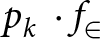 ${p_k}\, \cdot {f_ \in }$ represents extra spacing between frequencies in order to avoid frequency overlap.
 ${f_ \in }$ is the frequency resolution of the fast Fourier transform.
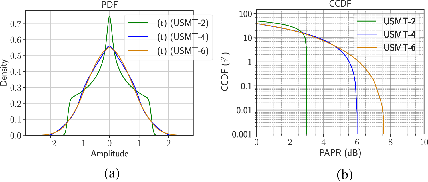
Relevant features are the statistical properties of the utilized signals, including the PDF and the CCDF. This facilitates the comparison of USMT signals with digitally modulated carriers. Figure 1 shows the PDF and CCDF of the USMT-2, USMT-4, and USMT-6 signals, which have 2, 4, and 6 frequency tones, respectively.
Statistical properties of the USMT-2 (2-Tones), USMT-4 and USMT-6 signals: (a) probability density function (PDF) of I(t); (b) complementary cumulative distribution function.

(1) Long description
PDF. The x-axis is labeled Amplitude, with tick labels at minus 2, minus 1, 0, 1 and 2. The y-axis is labeled Density, with tick labels from 0.0 to 0.7 in increments of 0.1. A legend lists I(t) (USMT-2), I(t) (USMT-4) and I(t) (USMT-6). Three smooth curves are plotted. The I(t) (USMT-2) curve has a narrow peak at amplitude 0, rising slightly above the 0.7 tick, then drops steeply; it shows visible shoulders around amplitude near minus 1 and plus 1 at a density a little above 0.2 and approaches near 0 density by about amplitude minus 1.6 and plus 1.6. The I(t) (USMT-4) curve peaks at amplitude 0 near density about 0.55, is broader than I(t) (USMT-2) and tapers toward near 0 density by about amplitude minus 2.3 and plus 2.3. The I(t) (USMT-6) curve is similar in shape to I(t) (USMT-4), with a peak at amplitude 0 near density about 0.55 and it also approaches near 0 density by about amplitude minus 2.3 and plus 2.3. CCDF. The x-axis is labeled PAPR (dB), with tick labels at 0, 2, 4, 6, 8 and 10. The y-axis is labeled CCDF (%), with tick labels at 100, 10, 1, 0.1, 0.01 and 0.001. A legend lists USMT-2, USMT-4 and USMT-6. Three curves decrease from left to right. The USMT-2 curve drops sharply around PAPR near 3 and reaches the bottom tick near 0.001 percent shortly after that. The USMT-4 curve decreases more gradually and then drops steeply around PAPR near 6, reaching near 0.001 percent around that value. The USMT-6 curve decreases more gradually than USMT-4 and extends farther right, dropping steeply between about PAPR 7 and 8 and reaching near 0.001 percent near that range.
It is shown that the more signal carriers are used, the more the PDF of the signal I(t) (in-phase) or Q(t) (in quadrature) is closer to a Gaussian distribution [Reference Silva dos Santos, Alleman, Reveyrand, Medrel, Chang, Sommet, Nébus, Prigent and Nallatamby9]. As a result, signals using the OFDM modulation scheme have a Gaussian-shaped PDF for the signals I(t) and Q(t). It is also noteworthy that CCDF facilitates the observation of the PAPR. For a USMT signal and under the assumption that all carriers have an identical amplitude, the PAPR of the signal is governed by equation (2), as illustrated in Fig. 1(b) [Reference Gillet, Bouslama, Teyssier, Prigent, Nallatamby and Quéré10, Reference Gibiino, Angelotti, Santarelli, Filicori and Traverso22].
 \begin{equation}{\text{PAPR }}{\left( {dB} \right)_{\text{ }}} = 10 \cdot {\text{log}}\left( {\text{N}} \right)\end{equation}
Consequently, the PAPR of the signal escalates with the number of signal carriers, thereby constraining the linear operating range of the transistor.
Adjacent channel power ratio (ACPR) is an important figure of merit for non-linear device characterization. It is defined as the ratio between the power of the main channel, the relevant part of the output signal, to the power in the adjacent channels due to the intermodulation products generated by the device [23]. Given the absence of overlap between the intermodulation products, as illustrated in Fig. 2, the ACPR can be calculated by measuring the power at each of the frequencies located in the adjacent channels and in the main channel (signal carriers).
Definition of ACPR using USMT-6 signal.

Figure 2 Long description
The plot illustrates power distribution across frequency bands, with the x-axis labeled Frequency in GHz and the y-axis labeled Power in decibels. The main channel bandwidth is flanked by two adjacent channel bandwidths. The reference power level, labeled P ref, is near the upper 20s decibels. Power levels in the main channel are marked by vertical bars clustering around 0 decibels, indicating a consistent power level below the reference. The adjacent channels, labeled Padj left and Padj right, show lower power levels. The plot demonstrates the adjacent channel power ratio, comparing power in the main channel to adjacent channels.
The ACPR for a USMT signal can be delineated through equation (3).
 \begin{equation}
{\text{ACPR }}{\left( {dB} \right)_{}} = 10 \cdot {\text{log}}\left( {\frac{{{{\mathop \sum}_{f \in {f_{{\text{carriers}}}}}}{P_{OUT}}\left( f \right){\text{ }}}}{{{{\mathop \sum}_{f \in {f_{{\text{adjacents}}}}}}{P_{OUT}}\left( f \right)}}} \right)\end{equation}
In this equation, 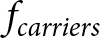 ${f_{carriers}}$ denotes the frequencies of the signal carriers, while
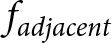 ${f_{adjacent}}$ signifies the frequencies of the intermodulation products generated in the channels adjacent to the band of the signal of interest.
Methodology
The device under test examined in this study is a pre-matched (Input/Ouput) at 29 GHz that serves as a process validation circuit 8 × 50 µm GaN HEMT on a wafer from UMSs. As shown in Figure 3, the transistor is pre-matched at the input and at the output.
Detail of the UMS GH-15 pre-matched transistor.

Figure 3 Long description
Layout view of the UMS GH-15 pre-matched transistor. The overall arrangement runs horizontally from left to right. On the far left, there are two rectangular contact pads positioned one above the other. These pads connect via horizontal metal traces to a central region containing two larger rectangular blocks arranged side by side. From the central blocks, metal traces extend to the right, connecting to two further rectangular contact pads, again arranged one above the other on the far right. Between the left pads and the central blocks and between the central blocks and the right pads, there are smaller square or rectangular elements positioned along the trace paths. The layout is broadly symmetrical about a horizontal axis. A short text label is visible at the top of the layout. The label is present but illegible at this resolution. No additional numerical ratings or node labels are clearly readable within the layout.
For a class AB quiescent point, the DC drain current ( ${I_{DS0}}$) is set at approximately 150 mA/mm and the drain voltage (
 ${V_{DS0}}$) at 20 V. The operating frequency is 29 GHz.
The device was tested using various signals, including USMT-2, USMT-4, and USMT-6, to assess its performance under diverse conditions. A comparison between the simulated and measured behavior of the device is presented for each signal.
Measurement setup
To characterize the transistor depicted in Figure 3, an on-probe measurement bench was developed and is illustrated in Figure 4. The test bench consists of a PNA-X, which is employed to measure the spectrum and power of the incident and reflected waves at the input and output of the DUT. The PNA-X N5245B vector network analyzer product from Keysight Technologies was used in this investigation.
PNA-X-based measurement setup for measuring the PAE using a multi-tones signal.

Figure 4 Long description
Measurement setup for characterizing a device under test, labeled DUT, using a network analyzer NVNA PNA-X operating at 50 GHz. At the top center, a laptop is connected via LAN or GPIB. Below the laptop, the NVNA PNA-X is centrally positioned, with connections labeled R1, R2, R3 and R4 extending from it. To the left, a signal generator is connected to an amplifier, which is linked to a bias-tee. This bias-tee is connected to a 50 ohm termination. On the right side, two power supplies are shown, each connected to a bias-tee. The bias-tees are connected to the DUT through GSG probes, with the DUT reference plane marked in blue. The connections labeled b subscript 1, a subscript 1, b subscript 2 and a subscript 2 are shown extending from the DUT. The NVNA reference plane is indicated in red, highlighting the measurement points. The setup is designed to measure the spectrum and power of incident and reflected waves at the input and output of the DUT.
In order to ascertain that the input and output power measurements are in the reference plane of the device indicated in blue (Fig. 4), a short-open-load-reciprocal on-probe calibration with an additional power calibration step was performed [Reference Reveyrand, Hernandez, Mons and Ngoya24].
The Rohde & Schwarz SMW200A vector signal generator was used to create the signal under consideration. A characteristic feature of this instrument is its ability to generate signals with arbitrary waveforms at high frequencies.
USMT-2, USMT-4, and USMT-6 were the signals used to characterize the device; Table 1 lists their corresponding frequencies [Reference Teyssier, Sombrin, Quéré, Laurent and Gizard25]. The signal bandwidth ranges from 201 kHz for the USMT-2 signal to 1.081 MHz for the USMT-8 signal, which indicates a narrowband signal.
USMT signal freq. used to characterize the DUT

Table 1 Long description
USMT signal frequencies used for device characterization are listed as six labeled points in gigahertz. Values rise steadily in small steps from 29.003000 GHz through 29.003201, 29.003403, 29.003609, and 29.003827 GHz to 29.004081 GHz. All frequencies are tightly grouped within roughly one thousandth of a gigahertz, indicating a narrow test band around 29.003 to 29.004 GHz. The lowest value is 29.003000 GHz and the highest is 29.004081 GHz. No units other than gigahertz or measurement uncertainty are provided, so precision and rounding limits cannot be confirmed.
The input range power is −10 dBm to 23 dBm. The transistor can operate in both the linear and saturation zones thanks to this range. As a result, the behavior of the transistor may be seen throughout these distinct operating zones.
Simulation process
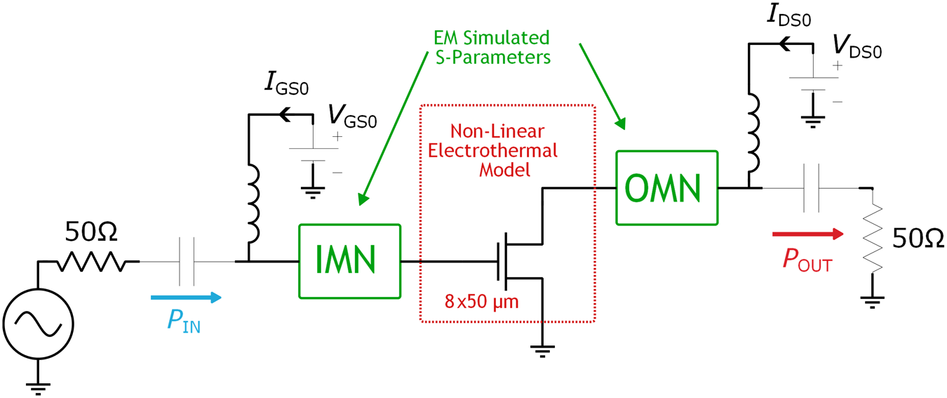
In the context of simulation, it is of paramount importance to meticulously replicate the measurement conditions within the Advanced Design System software. In order to achieve this, the transistor was simulated using the GH15 Design Kit supplied by UMS. Here, a GDS file was supplied by the foundry in order to simulate the tested device using an EM simulator. The schematic of this simulation is shown in Figure 5.
To achieve this, the input matching network (IMN) and OMN are simulated using the Momentum solver. The circuit was then simulated using the harmonic balance (HB) solver, and the nonlinear electrothermal model of the 8 × 50 µm component was updated with the S parameters of the IMN and OMN. Subsequently, the bias point was adjusted to reproduce the measurement conditions.
The S parameters of the simulated matching network were adjusted to match the results closer to the measured S parameters as a calibration step between the simulation and the measurements. In order to achieve this objective, a series of adjustments were implemented, including modifications to the active resistance of the transistor by using the spread parameters. This approach made it possible to simulate variances related to manufacturing and design processes. Another change involved modifying the electrothermal model’s component temperature, which was required due to a lack of direct thermal measurements. Finally, to model some minor manufacturing or measurements errors related to the passive circuit, transmission lines of approximately 10 µm were added.
It is essential to carry out a comprehensive study of the matching network simulations before analyzing the outcomes of the pre-matched transistor combining the transistor and the matching networks. This entails observing the matching procedures performed by these networks. In order to accomplish this objective, the S parameters of the transistor for a continuous drain current  ${I_{DS0}} = 60{\text{ }}mA$ (which corresponds to 150 mA/mm for an 8 × 50 µm transistor) and the S parameters of the matching networks were simulated, as illustrated in Figure 6 (a) for frequencies between 25 and 30 GHz.
Schematic of the electromagnetic co-simulation and circuit of the pre-matched component.

Figure 5 Long description
The circuit diagram includes a signal source connected to a 50 ohm resistor, followed by an input matching network labeled IMN. The IMN is connected to a non-linear electrothermal model with dimensions 8 times 50 micrometers. This model is connected to an output matching network labeled OMN. The circuit shows connections for current I subscript G50 and voltage V subscript G50 at both the input and output sides. The output side is connected to a 50 ohm resistor, with the output power labeled P subscript OUT. The diagram also includes labels for EM simulated S-parameters and P subscript IN at the input side.
(a) Comparison between  $S_{22}^{{\text{IMN}}}{\text{ }}$ and the conjugate of
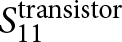 $S_{11}^{{\text{transistor}}}$. (b) Comparison between
 $S_{11}^{{\text{OMN}}}{\text{ }}$, conjugate of, and optimal impedances for PAE at 29 and 30 GHz.

Figure 6 Long description
Smith chart plots showing reflection coefficients. The horizontal axis represents normalized resistance and the vertical axis represents normalized reactance. In image A, the orange curve represents S22 for the input matching network and the green curve represents the conjugate of S11 for the transistor. In image B, the blue curve represents S11 for the output matching network and the green curve represents the conjugate of S22 for the transistor. Red and purple crosses mark the optimal gamma points for power added efficiency at 29 and 30 gigahertz, respectively. These points are located in the inductive region, indicating the desired impedance matching for optimal performance. The plots illustrate how the loci of S11 and S22 differ, with the optimal gamma points showing the target impedance for efficiency at the specified frequencies.
In the context of the IMN, impedance matching at the input stage is achieved through the presentation of the conjugate of S 11 of the transistor. Thus, it is necessary to compare the S 22 of the IMN with the conjugate of S 11 of the transistor when the drain is loaded by an OMN + 50 Ω. It can be observed that the IMN is matched with the input impedance of the transistor.
A similar approach can be used to analyze the OMN (Fig. 6(b)). It is necessary to compare the S 11 of the OMN with the conjugate of S 22 of the transistor when the gate is loaded by an IMN + 50 Ω. The latter is particularly crucial for transistor performance since load impedance affects features such as gain and efficiency.
A thorough examination of the figure indicates that the impedance presented by the OMN does not correspond to an impedance match, as the OMN’s S 11 does not equate to the conjugate of the transistor’s S 22. The OMN does not match the optimal power-added efficiency (PAE) value, according to a similar analysis of the output reflection coefficients at 29 and 30 GHz, which enable maximum PAE to be obtained.
It was thought that a load-null simulation analysis of this transistor would be significant because the device has not been matched to the load impedance and OMN prevents the achievement of maximal PAE. Consequently, the contours of the output power, gain, and PAE of this component can be observed in Figure 7.
Load-pull contours at 30 GHz (pre-matched). Optimal points:  ${P_{out}}$ (square), gain (circle), and PAE (triangle).

Figure 7 Long description
Load-Pull contours at 30 GHz (pre-matched). The image A showing a Smith chart for Pout (dBm) with reflection coefficient Gamma. The chart displays isocontours for constant output power levels, with optimal points marked: square for Pout at 31.24 dBm, circle for Gain at 31.24 dBm and triangle for PAE at 31.12 dBm. The image B showing a Smith chart for Gain (dB) with reflection coefficient Gamma. Isocontours represent constant gain levels, with optimal points marked: square for Pout at 7.42 dB, circle for Gain at 7.42 dB and triangle for PAE at 7.28 dB. The image C showing a Smith chart for PAE (%) with reflection coefficient Gamma. Isocontours indicate constant PAE levels, with optimal points marked: square for Pout at 37.48 percent, circle for Gain at 37.48 percent and triangle for PAE at 38.91 percent. The charts illustrate how the optimal points for Pout, Gain and PAE differ across the reflection coefficient plane, highlighting trade-offs between these metrics. The contours encode constant levels of Pout, Gain and PAE, showing regions of high performance and the separation of optimal points across the charts.
It is important to note that the optimal points are not located in the center of the Smith charts. However, the greatest PAE value is around 39%, whereas a transistor without matching networks simulation allows a PAE above 45%. This discrepancy can be attributed to the occurrence of losses within the matching networks, which in turn leads to a reduction in the resulting power and total gain.
The DUT under consideration is a test pattern (process control monitoring – PCM), so the impedance matching is not as precise as it would be for a PA. The gain block is employed to verify the proper functioning of the process.
Following these characterizations, a secondary simulation using the S parameters shown in Figures 7 allows for the analysis of the comprehensive circuit shown in Figure 4. Here, the HB simulation is used to incorporate third-order intermodulation products and harmonics. This simulation enables the observation of the nonlinear behavior of the device, a requirement for calculating the PAE. The simulation was executed by utilizing the USMT signals previously outlined, with a bias voltage of  ${V_{GS0}} = - 2.65{\text{ }}V$, thereby yielding a drain bias current of approximately 60 mA. The input power is measured within the range of −10 to 30 dBm, a range designed to encompass the linear and nonlinear characteristics of the device.
Results
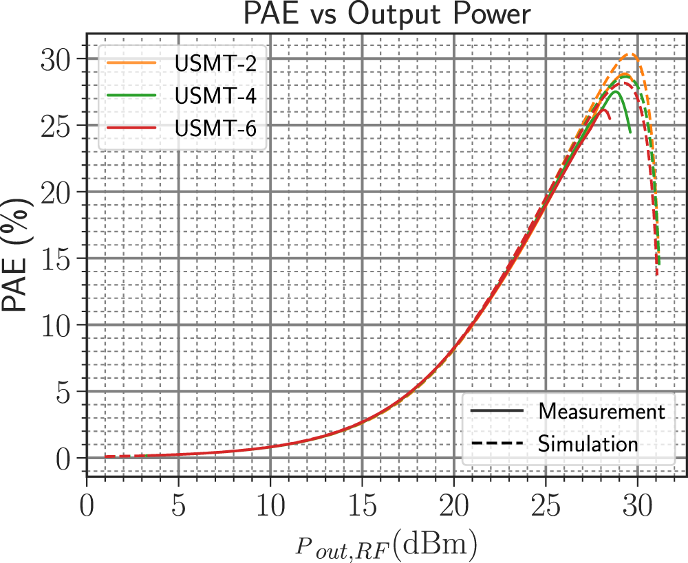
Transistors operate most efficiently when they are used close to their compression point. As illustrated in Figure 8, a comparison is made between the simulation and measurement of PAE utilizing USMT signals. The power values indicated in the following results correspond to their average values. The simulation of the USMT-2 signal demonstrates that for an output power of 29.5 dBm, a maximum PAE of 30.5% was obtained, and 29.5% for the measurement. An increase in the number of tones in the USMT signal necessarily implies a decrease in the maximum PAE value. For instance, the maximum PAE value obtained for the USMT-4 signal was 28.8% in the simulation and 28.2% in the measurement. For the USMT-6 signal, the maximum value obtained for the simulation was 28%, while the measurement yielded a maximum value of 26%.
Simulated (dashed lines) and measured (solid lines) PAE vs output power for different USMT configurations.

Figure 8 Long description
PAE vs Output Power Single line graph with a legend for USMT-2, USMT-4 and USMT-6 and a second legend showing Measurement (solid line) and Simulation (dashed line). The x-axis label is P out, RF (dBm). The x-axis shows labeled ticks at 0, 5, 10, 15, 20, 25 and 30. The y-axis label is PAE (percent). The y-axis shows labeled ticks at 0, 5, 10, 15, 20, 25 and 30. All series start near 0 percent at low output power and rise gradually up to about 15 dBm, then rise more steeply from about 15 dBm to about 28 dBm. USMT-2: The solid curve rises to about 20 percent near 25 dBm, reaches a peak near 30 dBm at about 29 to 30 percent, then drops by about 31 dBm to about 15 percent. The dashed curve follows a similar shape, peaking near 30 dBm at about 30 percent, then dropping by about 31 dBm to about 15 percent. USMT-4: The solid curve rises to about 20 percent near 25 dBm, reaches a peak near 29 to 30 dBm at about 28 percent, then drops by about 31 dBm to about 15 percent. The dashed curve peaks near 29 to 30 dBm at about 29 percent, then drops by about 31 dBm to about 15 percent. USMT-6: The solid curve rises to about 20 percent near 25 dBm, reaches a peak near 29 dBm at about 26 to 27 percent, then drops by about 31 dBm to about 14 to 15 percent. The dashed curve peaks near 29 to 30 dBm at about 28 percent, then drops by about 31 dBm to about 14 to 15 percent.
The observed discrepancies between measurement and simulation results can be attributed to the inherent challenges in reproducing the precise measurement conditions within the simulation framework. These challenges become particularly pronounced when the device operates close to its compression point, the nonlinear region under a complex modulated signal, or when dealing with a high PAPR signal.
A comparative analysis was performed using the USMT-2 (shown in orange), USMT-4 (shown in green), and USMT-6 (shown in red) signals. The device was simulated (dashed lines) and measured (solid lines) for each signal. As illustrated in Figure 9, the output power is depicted as a function of the input power.
Comparison between simulation (dashed lines) and measurements (solid lines) of the output power.

The results demonstrate that the device exhibits consistent behavior across all three signals, indicating that the gain and output power remain constant when an input power is applied during both simulation and measurement. However, a minor discrepancy emerges between the simulation and the measurement when the device operates within its linear range.
The average input power of the USMT-4 signal is constrained to a maximum value of  ${P_{in}} \approx 24{\text{ dBm}}$ and that of the USMT-6 signal is limited to
 ${P_{in}} \approx 21{\text{ dBm}}$. This is attributable to an increase in gate current (
 ${I_G}$) caused by a higher maximum instantaneous power. It is imperative to note that increasing the input power beyond this point can result in transistor damage.
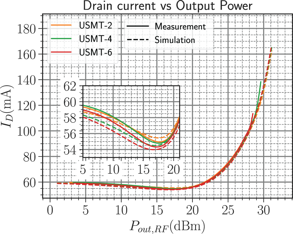
The analysis of the drain current depicted in Figure 10 reveals a degree of similarity among the various methods under consideration. In general, the drain current ( ${I_D}$) remains around 60 mA when the device operates in its linear region. However, a decrease in drain current is observable when the output power is approximately 10–20 dBm. This decay is associated with an imbalance in the capture and emission processes of the trap charges, suggesting an increase in the charge state as the input power increases. This phenomenon is attributable to the asymmetric time constant of the traps, which is proportional to the instantaneous excursion of the drain voltage [Reference Peng, Canfield and Allstot26, Reference Gibiino, Angelotti, Santarelli and Florian27].
Comparison between simulation (dashed lines) and measurements (solid lines) of the DC drain current (ID) consumption. A current drop is depicted in the inset.

Figure 10 Long description
Drain current vs Output Power Single plot with an inset. Legend entries: USMT-2, USMT-4, USMT-6, Measurement, Simulation. Measurement is shown with solid lines. Simulation is shown with dashed lines. Horizontal axis label: P out, RF (dBm). Tick labels shown at 0, 5, 10, 15, 20, 25, 30. Vertical axis label: I D (mA). Tick labels shown at 60, 80, 100, 120, 140, 160, 180. Main plot curves: USMT-2 measurement (solid): near 60 at low output power, decreases slightly to about 56 around 17 to 18, then increases; about 60 at 20, about 70 at 25, about 100 at 28 and about 165 near 31. USMT-2 simulation (dashed): closely follows the solid curve; near 60 at low output power, near 56 around 17 to 18, then rising to about 165 near 31. USMT-4 measurement (solid): near 60 at low output power, decreases to about 56 around 17 to 18, then increases; about 60 at 20, about 70 at 25, about 100 at 28 and about 165 near 31. USMT-4 simulation (dashed): closely follows the solid curve; near 60 at low output power, near 56 around 17 to 18, then rising to about 165 near 31. USMT-6 measurement (solid): near 60 at low output power, decreases to about 56 around 17 to 18, then increases; about 60 at 20, about 70 at 25, about 100 at 28 and about 165 near 31. USMT-6 simulation (dashed): closely follows the solid curve; near 60 at low output power, near 56 around 17 to 18, then rising to about 165 near 31. Inset plot: Inset horizontal axis shows tick labels 5, 10, 15, 20. Inset vertical axis shows tick labels 54, 56, 58, 60, 62. All six curves are shown again in the inset. Each curve slopes downward from about 59 to 60 near 5, reaches a minimum between about 54 and 56 around 16 to 18, then rises to about 57 to 59 near 20.
The PAPR increases as the number of signal carriers increases, which in fact causes the current excursion to climb at a certain output power. This can be attributed to the increase in recovery time that occurs in conjunction with an increase in PAPR [Reference Gibiino, Angelotti, Santarelli and Florian27]. For an output power greater than 20 dBm, the drain current increases with similar dynamics for all signals.
The device does not exhibit a pronounced decrease in DC drain current as a function of RF signal power when the signal’s PAPR is increased, because the device is a PCM whose output impedance matching does not result in load cycles with large voltage excursions. Such excursions are typically observed when the transistor operates near its efficiency optimum. Consequently, the DUT is not the optimally suitable option for demonstrating the effect of an increase in PAPR.
The existence of intermodulation products that do not overlap the signal carriers or other intermodulation products explains the use of the USMT signal in the nonlinear characterization of the transistor. The calculation of the ACPR is made by the analysis of the intermodulation products in the adjacent bands. As illustrated in Figure 11, a comparison is presented between the simulated and measured ACPR as a function of output power for various USMT signals.
Simulated (dashed lines) and measured (solid lines) ACPR (4 and 6 tones) and C/I (2 tones) vs output power for different USMT configurations.

Figure 11 Long description
ACPR vs Output Power Single line graph with two line-style categories and three labeled series. Legend at upper right: USMT-2, USMT-4, USMT-6. Legend at lower left: Measurement shown with a solid line; Simulation shown with a dashed line. Horizontal axis label: P out, RF (dBm). Tick labels shown at 16, 18, 20, 22, 24, 26, 28, 30. Left vertical axis label: ACPR (dB). Tick labels shown at 10, 15, 20, 25, 30, 35, 40, 45, 50. Right vertical axis label: C slash I (dB). Tick labels shown at 10, 15, 20, 25, 30, 35, 40, 45, 50. USMT-2 series: one solid curve and one dashed curve. The dashed curve starts near 46 dB at about 15 dBm and decreases to about 17 dB at 30 dBm. The solid curve starts near 43 dB at about 15 dBm and decreases to about 16 dB at 30 dBm, with a flatter segment around 28 dBm to 29 dBm near 21 dB. USMT-4 series: one solid curve and one dashed curve. The dashed curve starts near 41 dB at about 15 dBm and decreases to about 14 dB at 30 dBm. The solid curve starts near 40 dB at about 15 dBm and decreases to about 15 dB at 30 dBm. USMT-6 series: one solid curve and one dashed curve. The dashed curve starts near 40 dB at about 15 dBm and decreases to about 15 dB at 30 dBm. The solid curve starts near 39 dB at about 15 dBm and decreases to about 15 dB at 30 dBm. Two outlined ellipses appear near x around 18 to 19 and y around 32 to 37, with one arrow pointing right and one arrow pointing left.
A thorough examination of the simulations and measurements reveals a general tendency for the USMT-4 and USMT-6 signals. However, a notable discrepancy emerges for the USMT-2 signal within the linear zone. This discrepancy can be attributed to the sensitivity of the measurement configuration, which lacks the precision to accurately quantify the difference between carriers and intermodulation products above 40 dB. For output powers below 20 dBm, the slope of the results obtained is approximately 2 dB/dB, which is consistent with the behavior of the transistor in weakly nonlinear operation.
It has been observed that the ACPR value for the USMT-4 and USMT-6 signals is lower than the C/I ratio value of the USMT-2 signal. This is due to the fact that a higher PAPR implies greater distortion. A more thorough examination can be achieved by analyzing the output spectrum at the PA output plane for the various USMT signals.
A thorough analysis of the spectrum of the USMT-2 signal at the transistor output reveals two lines corresponding to the two signal tones and two lines corresponding to the two third-order intermodulation products. In order to ensure that all signals possess equivalent power, it is imperative to calibrate the amplitudes of each carrier. To illustrate, to have the same power as a USMT-2 signal, the amplitudes of the USMT-4 signal’s carriers must be reduced.
This adjustment ensures that four carriers of the USMT-4 signal attain the same power as two carriers of the USMT-2 signal. In a similar manner, the power of four third-order intermodulation products of the type 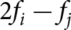 $2{f_i} - {f_j}$ generated by a USMT-4 signal is equivalent to the power of two intermodulation products of the type
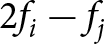 $2{f_i} - {f_j}$ generated by a USMT-2 signal. A USMT-6 signal can be analyzed using the same approach.
The increased number of tones indicates an increase in the number of third-order intermodulation products of the type 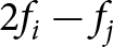 $2{f_i} - {f_j}$ in the adjacent bands, in addition to the additional intermodulation products of the type
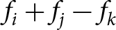 ${f_i} + {f_j} - {f_k}$, which have one-quarter of the power of the IMs in the adjacent bands of the type
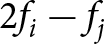 $2{f_i} - {f_j}$. Therefore, the relationship between the power of the
 ${\text{I}}{{\text{M}}_{\text{3}}}$s of a USMT-N signal and the power of the
 ${\text{I}}{{\text{M}}_{\text{3}}}$s of a USMT-2 signal can be calculated using equation (4). In this equation, N denotes the number of tones in the signal, R denotes the number of IMs of type
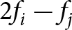 $2{f_i} - {f_j}$, and S represents the number of IMs of type
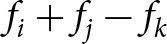 ${f_i} + {f_j} - {f_k}$. The quantities R and S depend on the number of signal carriers and the vector
 ${p_k}$ [Reference Silva Dos Santos28, Reference Gillet29].
 \begin{equation}{\frac{{{P_{I{M_3}}}\left( {{\text{USMT - N}}} \right)}}{{{P_{I{M_3}}}\left( {{\text{USMT - 2}}} \right)}}_{\text{ }}}\left( {{\text{dB}}} \right) = 10 \cdot \log \left( {\frac{{R + \frac{1}{4}S}}{N}} \right)\end{equation}
The increase in the number of tones does not result in a significant compression of the intended signal at the output, which may be neglected since the transistor operates within its linear region.
Consequently, an increase in the number of signal tones can be interpreted as an increase in the total power of the  $I{M_3}$ in the adjacent bands, while the output power of the signal remains constant. This indicates that, as the number of tones in the signal increases, ACPR decreases within the device’s linear zone, as illustrated in Figure 11. Equation (5) outlines how the ACPR of a USMT-N signal is determined based on this assumption.
In this equation, 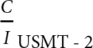 ${\frac{C}{I}_{{\text{USMT - 2}}}}$ is the
 $\frac{C}{I}$ ratio of the USMT-2 signal, IIP3 is the third-order input intercept point, and
 ${P_{in}}$ is the average input power.
 \begin{align}
{\text{ACPR }}\left({{\text{dB}}}\right) & = {\frac{C}{I}_{{\text{USMT - 2}}}} - 10 \cdot \log \left( {\frac{{R + \frac{1}{4}S}}{N}} \right)\nonumber\\
& = 2\left( {{\text{IIP3}} - {P_{in}}} \right) - 10 \cdot \log \left( {\frac{{R + \frac{1}{4}S}}{N}} \right)
\end{align}
As illustrated in Table 2, a comparative analysis has been conducted between the ACPR for the USMT-4 and USMT-6 signals and the C/I for the USMT-2 signal. This analysis has been performed using equation (5) and the simulated values. As previously mentioned, because of the bench’s sensitivity, the measured values were not used for comparison criteria.
Number of IM3 located in the adjacent bands of the signal, ratio between the power of the  ${\text{I}}{{\text{M}}_{\text{3}}}$ of the USMT-N signal in relation to the USMT-2 signal, and the calculated and simulated ACPR values for an output power of 15 dBm

Table 2 Long description
Adjacent-band third-order intermodulation results are listed for three USMT offsets at 15 dBm output power, including counts of products in two adjacent-band groupings, a power ratio relative to USMT minus 2, and calculated versus simulated ACPR or carrier-to-interference. USMT minus 2 has 2 products in the first grouping and 0 in the second, with a 0 dB power ratio and ACPR of 47 dB calculated versus 46.7 dB simulated. USMT minus 4 increases to 9 and 7 products, a 4.293 dB power ratio, and ACPR of 42.7 dB calculated versus 41.8 dB simulated. USMT minus 6 shows 20 and 30 products, a 6.612 dB power ratio, and ACPR of 40.4 dB calculated versus 40.6 dB simulated. Overall, more intermodulation products and higher relative intermodulation power correspond to lower ACPR, indicating worse adjacent-channel performance. Calculated and simulated ACPR values are close for all rows, differing by about 0.2 to 0.9 dB.
The minor discrepancy between the calculated and measured values can be attributed to the presence of compression in the output signal and intermodulation products, which contribute to increase the ACPR value. In the nonlinear region, signal compression becomes more relevant, and the ACPR no longer follows equation (5), as can be seen in Figure 11, where the ACPR curves for the USMT-4 and USMT-6 signals converge from Pout = 19 dBm.
Conclusion
The study entailed the characterization of a pre-matched HEMT transistor utilizing USMT-2, USMT-4, and USMT-6 signals around 29 GHz. This was achieved by comparing the results obtained with measurements and simulations of figures of merit, including output power, DC drain current, PAE, and ACPR. This approach was employed to characterize the linearity of the device. The findings suggest that the device demonstrates a more pronounced decline in drain current when a USMT signal with a higher number of frequencies is applied. This phenomenon can be attributed to the effects of traps and variations in signal dynamics. A decrease in the maximum PAE value was observed with an increase in the number of tones, a phenomenon that was confirmed through both measurements and simulations. The discrepancies observed between the simulation and the measurement, such as a lower PAE value for the measurement, are attributable to the challenges in reproducing the same conditions in the simulation as in the measurement, specifically at harmonic values. The measured values are also lower than those found when characterizing the transistor alone using load-pull because the matching networks have inherent losses and are not designed to obtain maximum PAE. An analysis of the ACPR reveals a high degree of concordance between the simulation and the measurement. One noteworthy finding is that the ACPR value decreases as the number of frequencies increases. This phenomenon is caused by signal dynamics; when the signal envelope’s maximum power increases, waveform distortion increases as well. Consequently, there is an increase in the number of intermodulation products in the adjacent bands.
Subsequent lines of research will entail the utilization of the USMT-8 signal for simulating the device, an examination of the NPR, and a mathematical analysis to ascertain the ACPR as a function of the number of tones in the nonlinear region. This approach will facilitate the development of a more comprehensive model. A salient point that merits attention is the necessity of conducting this comparative study using an unmatched device in accordance with the load-pull method.
Acknowledgements
The authors express their profound gratitude to United Monolithic Semiconductors for supplying the transistors that underwent characterization, as well as to the Direction Générale de l’Armement and the Centre National de la Recherche Scientifique (CNRS) for providing financial support under the GREAT Project. The experiments were carried out at the PLATINOM test facility of XLIM, a member of the CNRS RF-Net network (ANR-22-PEFT-0011).
Competing interests
The authors report no conflict of interest.

José Anderson Silva dos Santos received his Engineer Degree in Electrical Engineering in 2020 from the Federal Institute of Education, Science and Technology of Paraiba in João Pessoa, Brazil, and his Ph.D. degree in electronics from University of Limoges, France in 2024. He has been a teaching assistant at the University of Limoges since 2025. His research interests encompass RF microelectronics, instrumentation, data processing, digital communications, and microwaves.

Julien Alleman received the Engineering degree in Electrical Engineering from Toulouse INP-ENSEEIHT, France, in 2022. He received the Ph.D. degree in High-Frequency Electronics from the University of Limoges, France, in 2025. He conducted his doctoral research at the XLIM Institute. His research interests focus on the application of Artificial Intelligence to RF electronics, specifically utilizing deep neural networks for the modeling and reconstruction of load-pull measurement data for GaN HEMTs.

Margot Leventoux received the Engineering degree in Electrical Engineering in 2023 from ENSEA, Cergy, France. She is currently pursuing the Ph.D. degree in High-Frequency Electronics at the University of Limoges, France, since 2024. She conducts her doctoral research at the XLIM Institute. Her research interests include passive and active load-pull transistor measurements, as well as instrumentation and data processing.

Pierre Medrel received the Ph.D. degree in electronics from the University of Limoges, France, in 2014. From 2014 to 2015, he was a postdoctoral Scientist at the IMS laboratory, Bordeaux, France. He is now an associate professor with the XLIM institute, Limoges. His main field of interest is high-efficiency microwave PA architectures and non-linear device characterization.

Christophe Chang received the Ph.D. degree, under the Joint Doctoral Degree Program, from the XLIM Laboratory, University of Limoges, Limoges, France, and Thales Airborne Systems, Trappes, France. In 2004, he joined the XLIM Laboratory, University of Limoges, as a Post-Doctoral Researcher. He was involved in the characterization and the nonlinear modeling of the UMS GaInP/GaAs bipolar transistor. In 2005, he joined UMS SAS, where he is currently a Senior Modeling Engineer supporting the development of AsGa-based pHEMT power technologies such as PPH25X and PPH15X (technology support, characterization, and modeling). Since 2007, he has been involved in the support of the development of UMS GaN based technologies (characterization and nonlinear model building). He has participated in the development and the qualification of the 0.25 µm GH25 technology. Since 2014, he has been involved in the 0.15 µm GH15 technology development.

Fabien Courrèges received the B.S. degree in fundamental physics of the University of Orleans (France) in 1999, the M.S. degree in robotics of the University of Poitiers (France) in 2000 and the PhD degree in signal processing, robotics, and control at the University of Orl´eans in 2003. He is tenured assistant professor with the Intelligent Systems and Networks department of the XLIM research institute from the University of Limoges (France) since 2007. His main research concern is about systems and data modeling and processing for enabling design and control of smart and autonomous plants and systems.

Raphaël Sommet received the French aggregation degree in applied physics and the Ph.D. degree from the University of Limoges, Limoges, France, in 1991 and 1996, respectively. Since 1997, he has been a Permanent Researcher at XLIM, Institut de Recherche, Unités Mixtes de Recherche Centre National de la Recherche Scientifique 6172, Faculté des Sciences et Techniques, Université de Limoges, in the C2S2 team “Nonlinear Microwave Circuits and Subsystems.” His research interests concern heterojunction-bipolar-transistor device simulation, 3-D thermal finite element simulation, model order reduction, microwave circuit simulation, and generally the coupling of all physics-based simulation with circuit simulation.

Jean-Christophe Nallatamby received the Ph.D. degree in electronics from the University of Limoges, Limoges, France, in 1992. He is currently a Professor with the University of Limoges. His current research interests include the microwave, low-frequency noise characterization and modeling of high-speed semiconductor devices, characterization of charge-trapping effects in GaN HEMTs, and understanding its physical behavior using TCAD-based device simulation.