The interaction of gravity currents in a porous layer with a finite edge

Zhong Zheng

doi:10.1017/jfm.2023.638

The interaction of gravity currents in a porous layer with a finite edge

Published online by Cambridge University Press: 04 September 2023

Zhong Zheng

Show author details

Zhong Zheng*: Affiliation:
State Key Laboratory of Ocean Engineering, School of Naval Architecture, Ocean and Civil Engineering, Shanghai Jiao Tong University, Shanghai 200240, PR ChinaMOE Key Laboratory of Hydrodynamics, School of Naval Architecture, Ocean and Civil Engineering, Shanghai Jiao Tong University, Shanghai 200240, PR China
*: †Email addresses for correspondence: zzheng@alumni.princeton.edu, zhongzheng@sjtu.edu.cn

Article contents

Abstract
Introduction
Theoretical model
Time transition towards quasi-steady solutions
Summary and final remarks
Funding
Declaration of interests
References

Rights & Permissions

Abstract

The interactions of upper (lighter) and lower (heavier) gravity currents are closely related to fluid-phase resource recovery in porous layers and cleaning of confined spaces. The addition of a second current increases the sweep efficiency of fluid displacement. In this paper, we first derive two ordinary differential equations to describe the interaction of gravity currents in the quasi-steady regime. Two asymptotic regimes are identified, characterised by whether or not the two currents attach to each other, depending on whether the source fluxes are large enough. In the attached regime, a symmetry condition is also identified that describes whether or not the pumping and buoyancy forces balance each other. The model also leads to analytical solutions for the interface shape of the interacting currents in both the detached and attached regimes and for both symmetric and asymmetric currents. For symmetric currents, analytical solutions can also be obtained for the pressure distribution along cap rocks and the sweep efficiency of flooding processes. A particularly interesting aspect is that the displaced fluid remains quiescent at any steady state, regardless of whether the currents attach to each other. Correspondingly, the interface shape of the currents can be described by relatively simple equations and solutions, as if the currents propagate independently in unconfined porous layers. Time transition towards quasi-steady solutions is provided, employing time-dependent numerical solutions of two coupled partial differential equations for dynamic current interaction.

JFM classification

Low-Reynolds-number flows: Lubrication theory Geophysical and Geological Flows: Gravity currents

Information

Type: JFM Papers
Information: Journal of Fluid Mechanics , Volume 970 , 10 September 2023, A37
DOI: https://doi.org/10.1017/jfm.2023.638 [Opens in a new window]
Copyright: © The Author(s), 2023. Published by Cambridge University Press

1. Introduction

Gravity-driven flow in porous layers is of both fundamental and practical interest and finds many applications in nature and industry. For example, the invasion of a fluid layer into another one with distinct density is a typical situation when a gravity current is generated in a porous layer. Such a situation occurs when water invades into soils and sands in drainage and irrigation projects, when supercritical ${\rm CO}_2$ is injected into saline aquifer layers for permanent storage, when steam and water are pumped into rock formations for fluid-phase resource production and when acid gas and waste water are disposed into subsurface rock layers. The fundamentals of the gravity current spreading problem is the focus of a series of earlier studies that account for, for example, the influence of fluid drainage due to incompleteness of cap rocks (e.g. Acton, Huppert & Worster Reference Acton, Huppert and Worster2001; Pritchard, Woods & Hogg Reference Pritchard, Woods and Hogg2001; Farcas & Woods Reference Farcas and Woods2009; Woods & Farcas Reference Woods and Farcas2009; Liu, Zheng & Stone Reference Liu, Zheng and Stone2017) or existence of edges, geological faults and leaky wells (e.g. Boussinesq Reference Boussinesq1904; King & Woods Reference King and Woods2003; Neufeld, Vella & Huppert Reference Neufeld, Vella and Huppert2009; Hesse & Woods Reference Hesse and Woods2010; Gunn & Woods Reference Gunn and Woods2012; Zheng et al. Reference Zheng, Soh, Huppert and Stone2013; Kang et al. Reference Kang, Nordbotten, Doster and Celia2014; Cowton et al. Reference Cowton, Neufeld, White, Bickle, White and Chadwick2016; Momen et al. Reference Momen, Zheng, Bou-Zeid and Stone2017; Yu, Zheng & Stone Reference Yu, Zheng and Stone2017), the influence of flow confinement due to the finite thickness of a porous layer (e.g. Huppert & Woods Reference Huppert and Woods1995; Nordbotten & Celia Reference Nordbotten and Celia2006; Hesse et al. Reference Hesse, Tchelepi, Cantwell and Orr2007; MacMinn, Szulczewski & Juanes Reference MacMinn, Szulczewski and Juanes2010; Pegler, Huppert & Neufeld Reference Pegler, Huppert and Neufeld2014; Zheng et al. Reference Zheng, Guo, Christov, Celia and Stone2015; Hinton & Woods Reference Hinton and Woods2018; Zheng & Neufeld Reference Zheng and Neufeld2019; Zheng Reference Zheng2023), the influence of wetting and capillary forces as a current becomes unsaturated (e.g. Golding et al. Reference Golding, Neufeld, Hesse and Huppert2011; Zheng & Neufeld Reference Zheng and Neufeld2019; Zheng Reference Zheng2022), the influence of radially spreading configuration for fluid injection through vertical wells (e.g. Pattle Reference Pattle1959; Kochina, Mikhailov & Filinov Reference Kochina, Mikhailov and Filinov1983; Lyle et al. Reference Lyle, Huppert, Hallworth, Bickle and Chadwick2005; Nordbotten & Celia Reference Nordbotten and Celia2006; Guo et al. Reference Guo, Zheng, Bandilla, Celia and Stone2016; Hinton Reference Hinton2020; Hutchinson, Gusinow & Worster Reference Hutchinson, Gusinow and Worster2023) and the influence of a lubricating fluid layer that is related to the grounding line dynamics between marine ice sheets and shelves (e.g. Pegler & Worster Reference Pegler and Worster2013; Pegler et al. Reference Pegler, Kowal, Hasenclever and Worster2013; Kowal & Worster Reference Kowal and Worster2015, Reference Kowal and Worster2019a,Reference Kowal and Worsterb, Reference Kowal and Worster2020). A recent review is also available with a focus on the influence of boundaries on the flow of gravity currents (Zheng & Stone Reference Zheng and Stone2022). Another report is available on the influence of inertia (Linden Reference Linden2012), when the propagation of a current is typically controlled by a Fr condition at the front. Another typical situation is when laminar plumes are generated with equally important horizontal and vertical advective flows. Such flow patterns also broadly appear in near-field regions of heating sources in geothermal formations and near-field regions of injection points and geological faults during the disposal and leakage of buoyant fluids (e.g. Wooding Reference Wooding1963; Hewitt, Peng & Lister Reference Hewitt, Peng and Lister2020).

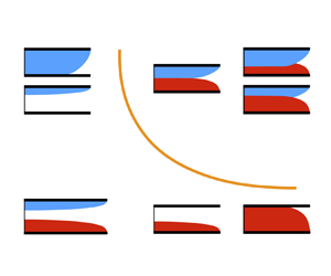
Among the very many interesting and important topics of gravity-driven flow in porous layers, we study the interaction of two gravity currents in this paper, as sketched in figure 1. Such a situation is closely related to the practice of cleaning confined spaces and enhanced recovery of fluid-phase resources. By introducing a second current, either heavier or lighter, compared with the ambient fluid, the sweep efficiency (defined later in (2.38)) of the flooding flow is expected to increase. We are particularly interested in characterising the interface shape of the two currents and assessing the degree of increase in sweep efficiency by introducing a second current. Meanwhile, in a broader context, study of the interaction and coalescence of thin capillary films (e.g. Ristenpart et al. Reference Ristenpart, McCalla, Roy and Stone2006; Hernandez-Sanchez et al. Reference Hernandez-Sanchez, Lubbers, Eddi and Snoeijer2012; Zheng et al. Reference Zheng, Fontelos, Shin, Dallaston, Tseluiko, Kalliadasis and Stone2018; Kaneelil et al. Reference Kaneelil, Pahlavan, Xue and Stone2022) and hydraulic fractures (e.g. O'Keeffe et al. Reference O'Keeffe, Zheng, Huppert and Linden2018) has also made promising progresses in recent years.

Figure 1.

The interaction of gravity currents generated by simultaneous injection of two fluids of distinct density into a porous layer of permeability $k$, porosity $\phi$, length $x_e$ and thickness $h_0$. A steady state is reached when the rate of injection equals that of drainage at the edge. Two regimes of quasi-steady interaction naturally appear: (a) ‘detached’ currents and (b) ‘attached’ currents, including both symmetric and asymmetric currents. (c) A heavier current of shape $h_1(x)$ is injected at area rate $q_1$ and drains also at the same rate $q_1$ at an edge ($x=x_e$), while a lighter current of shape $h_2(x)$ is injected at rate $q_2$ and drains also at rate $q_2$ at $x=x_e$. The density, viscosity and pressure of the three fluids are denoted by $\rho _i$, $\mu _i$ and $p_i(x,z)$, respectively, with $i=\{1,2,3\}$. At higher injection rates, a detaching location $x=x_d$ appears, leading to an attached region ($x \in [0,x_d]$) and a detached region ($x \in (x_d, x_e]$).

We are aware of a previous work in which two immiscible gravity currents are injected into an unconfined porous medium, displacing a third ambient fluid (e.g. air) that is lighter than either of the injected fluids (Woods & Mason Reference Woods and Mason2000). The current work, nevertheless, investigates a different situation of gravity current interaction, as shown in figure 1. Some novel aspects of the current work are highlighted as follows:

(i) The two currents are both heavier than the ambient fluid in the earlier work of Woods & Mason (Reference Woods and Mason2000). In the current work, the density of the ambient fluid lies between that of the two injected fluids, such that a heavier current is generated and spreads along the base, while another lighter current is generated and spreads along the top. This is consistent with the practice of enhancing oil recovery, for example, when water and ${\rm CO}_2$ (or steam) currents are injected into a rock formation to displace oil, simultaneously or alternately, as the density of oil lies between that of ${\rm CO}_2$ and water at reservoir conditions, i.e. $\rho _{\text {CO2}} < \rho _{{oil}} < \rho _{{water}}$ (e.g. Lake Reference Lake1989).
(ii) The porous layer is assumed to be infinitely long in Woods & Mason (Reference Woods and Mason2000), so the two currents interact while continuing to propagate. In the current work, the porous layer has a finite length, such that both the heavier and lighter currents reach an edge at a finite location, which mimics the existence of a production well or geological fault (e.g. Golding et al. Reference Golding, Neufeld, Hesse and Huppert2011; Zheng et al. Reference Zheng, Soh, Huppert and Stone2013; Yu et al. Reference Yu, Zheng and Stone2017). Accordingly, the flow becomes quasi-steady, when the rate of injection equals the rate of drainage. This configuration also mimics the core-flooding experimental set-up and can possibly provide insights into the fundamentals of multi-phase Darcy flow in co-flooding situations.
(iii) The porous layer is assumed to be infinitely deep in the model problem of Woods & Mason (Reference Woods and Mason2000), so the propagation of the two currents always remains unconfined. In the current work, however, the porous layer takes a finite thickness. This is consistent with many flow situations in sedimentary formations, which naturally exhibit layered patterns with significant permeability contrasts across layers. Accordingly, the flow becomes confined, when the currents attach to both the top and base of the porous layer (e.g. Huppert & Woods Reference Huppert and Woods1995; Pegler et al. Reference Pegler, Huppert and Neufeld2014; Zheng et al. Reference Zheng, Guo, Christov, Celia and Stone2015). At higher injection rates, the currents can also attach to each other and interact.
(iv) The model and solutions turn out to be clean and simple. In the sharp-interface regime, analytical solutions can be obtained for the interface shape of the interacting currents, the background pressure distribution along the cap rock and the sweep efficiency in cleaning and resource recovery applications. This is mainly due to the fact that the motion of the ambient fluid can still be neglected in these quasi-steady flow situations, even when the heavier and lighter gravity currents are both confined in a porous layer with finite thickness.

This paper is structured as follows. A theoretical model is first proposed in § 2 to describe the profile shape of the interacting currents, based on the assumption of quasi-steady sharp-interface flows. Asymptotic solutions are then provided for the profile shape of the two currents in both the detached and attached regimes and for both symmetric and asymmetric currents. For symmetric currents, analytical solutions are also provided for the background pressure distribution and sweep efficiency of co-flooding flows. Then in § 3, time transition towards quasi-steady solutions is provided, employing time-dependent numerical solutions of two coupled partial differential equations (PDEs) for dynamic current interaction. We close the paper in § 4 with a brief summary and remarks on model assumptions and potential implications.

2. Theoretical model

2.1. Governing equations

The model problem is sketched in figure 1: two gravity currents are generated in a porous layer of finite thickness $h_0$, with the heavier one spreading along the base and lighter one spreading along the top. A steady state is reached when the rate of fluid injection equals that of drainage at a finite edge $x=x_e$ for both the heavier and lighter gravity currents. The porous layer is assumed to be horizontal, homogeneous and isotropic, with permeability and porosity denoted by $k$ and $\phi$, respectively. The viscosity and density of the injecting fluids 1 and 2 are denoted by $\mu _1$, $\mu _2$, $\rho _1$ and $\rho _2$, respectively, and for the displaced/ambient fluid 3, they are denoted by $\mu _3$ and $\rho _3$. It is assumed that $\rho _1 > \rho _3 > \rho _2$, such that a heavier current is generated between fluids 1 and 3, while a lighter one is generated between fluids 2 and 3, as shown in figure 1. The propagation of the currents is driven by buoyancy, due to the density difference between the injecting and displaced fluids. We only consider the Cartesian configuration in this work, recognising that the concept also applies for flow in the radial configuration.

We focus on the interaction of the heavier and lighter gravity currents. We expect that they remain separated from each other at lower injection rates, as shown in figure 1(a). At higher injection rates, in contrast, they attach to each other, when the displaced fluid 3 is completely pushed downstream towards the edge, as shown in figure 1(b). We are particularly interested in the shape of the fluid–fluid interfaces, which remains an open question for the theory of gravity-driven flows. It is also of interest to evaluate the amount of fluid 3 that can be swept out of the porous layer, which is related to the sweep efficiency in the practice of fluid-phase resource recovery and cleaning of confined spaces.

It is also assumed that both currents are long and thin, such that the vertical component of the Darcy velocity is negligible compared with the horizontal component. This is a typical situation of flow in shallow layers of soils, sands and porous rocks, and is closely related to the practice of oil and gas recovery, pollutant migration, geological sequestration of ${\rm CO}_2$ and drainage and irrigation. This assumption has been employed in earlier studies of the flow of a single gravity current and verified experimentally based on time-dependent measurement of the profile shape and frontal location in both Hele-Shaw cells (e.g. Huppert & Woods Reference Huppert and Woods1995; Woods & Mason Reference Woods and Mason2000; King & Woods Reference King and Woods2003; Neufeld et al. Reference Neufeld, Vella and Huppert2009; Hesse & Woods Reference Hesse and Woods2010; Zheng et al. Reference Zheng, Soh, Huppert and Stone2013; Zheng, Christov & Stone Reference Zheng, Christov and Stone2014; Pegler et al. Reference Pegler, Bain, Huppert and Neufeld2015; Zheng, Ghodgaonkar & Christov Reference Zheng, Ghodgaonkar and Christov2021) and packed-bead systems (e.g. Pegler et al. Reference Pegler, Huppert and Neufeld2014).

Finally, the influence of interfacial tension and fluid mixing is neglected in the current work, assuming that sharp interfaces are created and maintained between the different fluids. This assumption has also been verified experimentally in the aforementioned studies. It is of interest to note that wetting and capillary forces can significantly alter the behaviour of gravity current flows and lead to gradual change of fluid saturations rather than to sudden change across sharp interfaces (e.g. Golding et al. Reference Golding, Neufeld, Hesse and Huppert2011; Zheng & Neufeld Reference Zheng and Neufeld2019). Fluid mixing can also alter the behaviour of miscible currents (e.g. Nijjer, Hewitt & Neufeld Reference Nijjer, Hewitt and Neufeld2022), which can be of interest for future investigations.

Under the assumption of quasi-steady one-dimensional sharp-interface flow, the pressure distribution within the three fluid layers is hydrostatic and follows

(2.1a)

\begin{gather} p_1(x,z) = p_0(x) - \rho_1 g z, \quad\mbox{for}\ 0 \leq z < h_1(x), \end{gather}

(2.1b)

\begin{gather}p_3(x,z) = p_0(x) - \Delta \rho_1 g h_1 - \rho_3 g z, \quad\mbox{for}\ h_1(x) \leq z < h_0-h_2(x), \end{gather}

(2.1c)

\begin{gather}p_2(x,z) = p_0(x) - \Delta \rho_1 g h_1 - \Delta \rho_2 g (h_0 - h_2) - \rho_2 g z, \quad \mbox{for}\ h_0-h_2(x) \leq z \leq h_0, \end{gather}

where $p_0(x)$ denotes the distribution of the background pressure along the base $z=0$ and the density differences are defined as $\Delta \rho _1 \equiv \rho _1 - \rho _3 > 0$ and $\Delta \rho _2 \equiv \rho _3 - \rho _2 > 0$. The horizontal velocity of the fluids within each layer can then be estimated based on Darcy's law:

(2.2a)

\begin{gather} u_1(x) ={-}\frac{k}{\mu_1} \frac{\partial p_1}{\partial x} ={-}\frac{k}{\mu_1} \frac{{\rm d}p_0}{{\rm d}x}, \end{gather}

(2.2b)

\begin{gather}u_3(x) ={-}\frac{k}{\mu_3} \frac{\partial p_3}{\partial x} ={-}\frac{k}{\mu_3} \left(\frac{{\rm d}p_0}{{\rm d}x} - \Delta \rho_1 g \frac{{\rm d}h_1}{{\rm d}x}\right), \end{gather}

(2.2c)

\begin{gather}u_2(x) ={-}\frac{k}{\mu_2} \frac{\partial p_2}{\partial x} ={-}\frac{k}{\mu_2} \left(\frac{{\rm d}p_0}{{\rm d}x} - \Delta \rho_1 g \frac{{\rm d}h_1}{{\rm d}x} + \Delta \rho_2 g \frac{{\rm d}h_2}{{\rm d}x}\right). \end{gather}

Meanwhile, at any steady state, local continuity requires that

(2.3a,b)

\begin{equation} h_1 u_1 = q_1 \quad\mbox{and}\quad h_2 u_2 = q_2, \end{equation}

at any location $x$, where $q_1$ and $q_2$ denote the (area) rate of accumulation of the heavier and lighter fluids into the porous layer, respectively. Conservation of volume, in addition, requires that

(2.4)

\begin{equation} h_1 u_1 + h_2 u_2 + (h_0 - h_1 - h_2) u_3 =q_1+q_2, \end{equation}

for any $x$. Based on (2.3) and (2.4), we then arrive at

(2.5)

\begin{equation} (h_0 - h_1 - h_2) u_3 = 0. \end{equation}

Physically, (2.5) indicates that the flux of the ambient fluid is zero at steady state, which also leads to two solution branches of the quasi-steady flow, depending on the profile shape of the currents:

(i) Branch (i): $h_0 - h_1 - h_2 > 0$, when the heavier and lighter currents remain detached, separated by an ambient layer of finite thickness.
(ii) Branch (ii): $h_0 - h_1 - h_2 = 0$, when the heavier and lighter currents attach to each other, with the ambient fluid being squeezed downstream during the time transition (towards quasi-steady states).

2.1.1. Detached region

When the currents are separated ($h_0 - h_1 - h_2 > 0$), we immediately obtain

(2.6)

\begin{equation} u_3 = 0 \end{equation}

in a detached region where $h_1+h_2 < h_0$. This can occur when the currents remain completely separated within the entire domain at lower injection rates. This can also occur only in a local region close to the edge of drainage at higher injection rates (while the currents remain attached in a region close to the inlet). Equation (2.6) is an interesting and important result, which indicates that the ambient fluid 3 remains quiescent within the entire domain for these quasi-steady sharp-interface flows. Physically, this is a consequence when fluid injection and drainage balance each other.

In addition, with (2.2b) and (2.6), the gradient of the background pressure becomes available as

(2.7)

\begin{equation} \frac{{\rm d}p_0}{{\rm d}x} = \Delta \rho_1 g \frac{{\rm d}h_1}{{\rm d}x}, \end{equation}

which can be substituted back into (2.2) for the Darcy velocities $u_1(x)$ and $u_2(x)$:

(2.8a)

\begin{gather} u_1 (x) ={-}\frac{\Delta \rho_1 g k}{\mu_1} \frac{{\rm d}h_1}{{\rm d}x}, \end{gather}

(2.8b)

\begin{gather}u_2 (x) ={-}\frac{\Delta \rho_2 g k}{\mu_2} \frac{{\rm d}h_2}{{\rm d}x}. \end{gather}

Equations (2.8a,b) can then be substituted into (2.3a,b) for the interface shape $h_1(x)$ and $h_2(x)$ as

(2.9a)

\begin{gather} -\frac{\Delta \rho_1 g k}{\mu_1} h_1 \frac{{\rm d}h_1}{{\rm d}x} = q_1, \end{gather}

(2.9b)

\begin{gather}- \frac{\Delta \rho_2 g k}{\mu_2} h_2\frac{{\rm d}h_2}{{\rm d}x} = q_2. \end{gather}

The ordinary differential equations (ODEs) (2.9a,b) can then be solved, together with appropriate boundary conditions at the location of the edge for both the heavier and lighter currents, e.g. the zero-thickness condition:

(2.10a,b)

\begin{equation} h_1 (x_e) = 0 \quad \mbox{and}\quad h_2 (x_e) = 0. \end{equation}

It is suggested based on (2.9a,b) and (2.10a,b) that the interface shape of the heavier current $h_1(x)$ and that of the lighter current $h_2(x)$ are independent of each other. Physically, this is due to the fact that the ambient fluid remains quiescent for such quasi-steady flows, as indicated by (2.6).

2.1.2. Attached region

When the currents attach to each other ($h_0 - h_1 - h_2 = 0$), (2.4) reduces to

(2.11)

\begin{equation} h_1 u_1 + h_2 u_2 = q_1+q_2. \end{equation}

Substituting (2.2a,c) into (2.11), we obtain the pressure gradient along the base as

(2.12)

\begin{equation} \frac{{\rm d}p_0}{{\rm d}x} = \frac{\dfrac{\Delta \rho g k}{\mu_2} (h_0-h_1)\dfrac{{\rm d}h_1}{{\rm d} x} - (q_1+q_2)}{\dfrac{k}{\mu_1}h_1 + \dfrac{k}{\mu_2}(h_0-h_1)}, \end{equation}

where $\Delta \rho \equiv \Delta \rho _1 + \Delta \rho _2 = \rho _1 - \rho _2 >0$. Equation (2.12) is then substituted back into (2.2a) and (2.3a) to provide

(2.13)

\begin{equation} \frac{\Delta \rho g k}{\mu_2} h_1(h_0-h_1) \frac{{\rm d}h_1}{{\rm d} x} + q_1M(h_0-h_1) - q_2h_1 = 0, \end{equation}

where $M \equiv \mu _1/\mu _2$ is the viscosity ratio of the two currents. The ODE (2.13) can then be solved subject to

(2.14)

\begin{equation} h_1(x_d) = h_d, \end{equation}

for the profile shape of the heavier current $h_1(x)$ in the attached region, with $(x_d, h_d)$ denoting the location where the three fluids meet and can be obtained by studying the detached solutions for $x \in [x_d,x_e]$ at higher injection rates (as we show later for the rescaled system). Once $h_1(x)$ is known, the profile shape $h_2(x) = h_0 - h_1(x)$ can also be obtained for the lighter current in the attached region. We have thus completed the model for the profile shape of the interacting currents in both the detached and attached regions.

2.2. Non-dimensionalisation

It is standard first to non-dimensionalise the governing equations and conditions before discussing the solutions. We first study the the detached region ($h_1+h_2 < h_0$) and rescale ODEs (2.9a,b) and boundary conditions (2.10a,b) for the profile shape of the detached currents. The dimensionless length and height are defined as

(2.15a–c)

\begin{equation} \bar{x} \equiv x/x_e, \quad\bar{h}_1 \equiv h_1/h_0 \quad \mbox{and}\quad \bar{h}_2 \equiv h_2/h_0, \end{equation}

with characteristic length and height scales chosen as $x_e$ and $h_0$, the length and thickness of the porous layer. Using these scalings, we arrive at the following dimensionless form of ODEs (2.9a,b):

(2.16a)

\begin{gather} - \bar{h}_1 \frac{{\rm d} \bar{h}_1}{{\rm d} \bar{x}} = \bar{q}_1, \end{gather}

(2.16b)

\begin{gather}- \bar{h}_2\frac{{\rm d}\bar{h}_2}{{\rm d} \bar{x}} = \bar{q}_2, \end{gather}

where two dimensionless injection rates $\bar {q}_1$ and $\bar {q}_2$ are found to be essential and defined as

(2.17a,b)

\begin{equation} \bar{q}_1 \equiv \frac{q_1 \mu_1 x_e}{\Delta \rho_1 g k h_0^2} \quad \mbox{and}\quad \bar{q}_2 \equiv \frac{q_2 \mu_2 x_e}{\Delta \rho_2 g k h_0^2}. \end{equation}

Physically, $\bar {q}_1$ and $\bar {q}_2$ also measure the competition between injection-driven and buoyancy-driven flows in determining the interface shape of the quasi-steady currents.

The dimensionless boundary conditions, meanwhile, can be obtained as

(2.18a,b)

\begin{equation} \bar{h}_1 (1) = 0 \quad \mbox{and}\quad \bar{h}_2 (1) = 0. \end{equation}

We are now ready to discuss the solutions for the interface shape of the heavier and lighter gravity currents $\bar {h}_1(\bar {x})$ and $\bar {h}_2(\bar {x})$ by solving (2.16a,b), subject to (2.18a,b). The solutions are under the influence of two dimensionless parameters $\bar {q}_1$ and $\bar {q}_2$, as defined in (2.17a,b) and summarised in table 1. In particular, we expect that the heavier and lighter currents remain separated at lower injection rates (to be quantified later), while they approach and attach to each other at higher injection rates.

Table 1.

Definition and physical description of the dimensionless parameters $\bar {q}_1$, $\bar {q}_2$, $G$ and $\delta$ for the interaction of heavier and lighter gravity currents that also drain at a finite edge.

Similarly, we can also non-dimensionalise ODEs (2.13) and boundary conditions (2.14) in the attached region ($h_1+h_2 = h_0$) to provide

(2.19)

\begin{equation} \left(1+\frac{1}{G}\right) \frac{1}{\bar{q}_2} \bar{h}_1(1 - \bar{h}_1) \frac{{\rm d}\bar{h}_1}{{\rm d} \bar{x}} + \frac{1}{G}\frac{\bar{q}_1}{\bar{q}_2}(1-\bar{h}_1) - \bar{h}_1 = 0 \end{equation}

and

(2.20)

\begin{equation} \bar{h}_1(\bar{x}_d) = \bar{h}_{d}, \end{equation}

where $\bar {x}_d \equiv x_d/x_e \in [0,1]$ and $\bar {h}_{d} \equiv h_{d}/h_0 \in [0,1]$. We expect that $(\bar {x}_d, \bar {h}_d)$ only depends on $\bar {q}_1$ and $\bar {q}_2$ based on solutions to ODEs (2.16a,b) in the detached region. Meanwhile, an extra dimensionless parameter $G$ is identified in (2.19), defined as

(2.21)

\begin{equation} G \equiv \frac{\Delta \rho_2}{\Delta \rho_1} = \frac{\rho_3 - \rho_2}{\rho_1 - \rho_3}. \end{equation}

Physically, $G$ represents the buoyancy ratio of the two currents. It is indicated that solutions for the profile shape $\bar {h}_1(\bar {x})$ and $\bar {h}_2(\bar {x})$ are under the influence of three dimensionless parameters, $\bar {q}_1$, $\bar {q}_2$ and $G$, the physical meanings of which are summarised in table 1. The aspect ratio $\delta \equiv h_0/x_e$ of the porous layer is also included in table 1, which is related to the applicability of the one-dimensional flow assumption, as we remark in § 4.1.

2.3. The ‘detached’ and ‘attached’ regimes

We next discuss in detail the asymptotic solutions for the shape of the interacting gravity currents. Both the ‘detached’ and ‘attached’ regimes are addressed, defined based on whether the heavier and lighter currents remain separated or attach to each other within the domain of the porous layer.

2.3.1. The ‘detached’ regime

At lower injection rates, defined by $(\bar {h}_1 + \bar {h}_2)|_{\bar {x} = 0} < 1$, the heavier and lighter gravity currents remain separated from each other, which leads to a ‘detached’ regime. Analytical solutions can be obtained for the shape of the heavier and lighter gravity currents by solving ODEs (2.16a,b), subject to (2.18a,b), which provides

(2.22a)

\begin{gather} \bar{h}_1(\bar{x}) = \left[2\bar{q}_1 (1-\bar{x})\right]^{1/2}, \end{gather}

(2.22b)

\begin{gather}\bar{h}_2(\bar{x}) = \left[2\bar{q}_2 (1-\bar{x})\right]^{1/2}. \end{gather}

An equivalent version of this parabolic solution has been derived previously for a single current that drains at a finite edge and verified experimentally (e.g. Hesse & Woods Reference Hesse and Woods2010; Golding et al. Reference Golding, Neufeld, Hesse and Huppert2011). Correspondingly, the thicknesses of the heavier and lighter currents at the entrance ($\bar {x} = 0$) of the porous layer are

(2.23a,b)

\begin{equation} \bar{h}_1(0) = (2\bar{q}_1)^{1/2}\quad \mbox{and}\quad \bar{h}_2(0) = (2\bar{q}_2)^{1/2}, \end{equation}

respectively.

It is also necessary to verify the requirement of $(\bar {h}_1 + \bar {h}_2)|_{\bar {x} = 0} < 1$ for this detached regime based on (2.23), which leads to

(2.24)

\begin{equation} \bar{q}_1^{1/2} + \bar{q}_2^{1/2} < 2^{{-}1/2}. \end{equation}

Physically, (2.24) suggests that the detached regime is obtained when the injection rates are small enough and provides an quantitative description. This regime is allocated in a regime diagram of figure 2.

Figure 2.

The regime diagram of detached and attached currents, including symmetric and asymmetric currents, separated by a curve $\bar {q}_1^{1/2} + \bar {q}_2^{1/2} = 2^{-1/2}$ of the injection rates of the heavier and lighter currents. The corresponding regimes for unconfined and confined single currents are also depicted along the horizontal and vertical axes as $\bar {q}_1 \to 0^+$ or as $\bar {q}_2 \to 0^+$.

2.3.2. The ‘attached’ regime

At higher injection rates, when $(\bar {h}_1 + \bar {h}_2)|_{\bar {x} = 0} = 1$, the heavier and lighter currents attach to each other within the porous layer, corresponding to an ‘attached’ regime. The region of attachment ($\bar {x} \in [0, \bar {x}_d]$), as defined by where $\bar {h}_1(\bar {x}) + \bar {h}_2(\bar {x}) = 1$, starts from the location of the entrance ($\bar {x} = 0$) and ends at a detaching point ($\bar {x} = \bar {x}_d \in (0,1)$). Correspondingly, the thicknesses of the heavier and lighter currents at the detaching point $\bar {x} = \bar {x}_d$ are given by

(2.25a)

\begin{gather} \bar{h}_1(\bar{x}_d) = \left[2\bar{q}_1 (1-\bar{x}_d)\right]^{1/2}, \end{gather}

(2.25b)

\begin{gather}\bar{h}_2(\bar{x}_d) = 1 - \left[2\bar{q}_1 (1-\bar{x}_d)\right]^{1/2}, \end{gather}

and, by definition, $\bar {h}_d \equiv \bar {h}_1(\bar {x}_d)$.

Within the detached region $\bar {x} \in (\bar {x}_d,1]$, in contrast, the heavier and lighter gravity currents remain separated, as sketched in figure 1(b). The shape of the interface $h_1(x)$ and $h_2(x)$ can still be described by (2.9a,b), assuming that the location of detachment $x=x_d$ is sufficiently far away from the edge $x=x_e$ and the flow is still one-dimensional. It can be shown that the shape of the heavier and lighter currents in the detached region ($\bar {x} \in [\bar {x}_d,1]$) can still be described by (2.22); see Appendix A. Correspondingly, the thicknesses of the heavier and lighter currents at the detaching point $\bar {x} = \bar {x}_d$ become

(2.26a)

\begin{gather} \bar{h}_{1}(\bar{x}_d) = \left[2\bar{q}_1 (1-\bar{x}_d)\right]^{1/2}, \end{gather}

(2.26b)

\begin{gather}\bar{h}_{2}(\bar{x}_d) = \left[2\bar{q}_2 (1-\bar{x}_d)\right]^{1/2}. \end{gather}

Based on (2.25b) and (2.26b), the location of detachment $\bar {x} = \bar {x}_{d}$ can then be determined by solving

(2.27)

\begin{equation} 1 - \left[2\bar{q}_1 (1-\bar{x}_d)\right]^{1/2} = \left[2\bar{q}_2 (1-\bar{x}_d) \right]^{1/2}, \end{equation}

which provides

(2.28)

\begin{equation} \bar{x}_d = 1 - 1\left/2\left(\bar{q}_1^{1/2} + \bar{q}_2^{1/2}\right)^2.\right. \end{equation}

The thickness of the currents $\bar {h}_{1}(\bar {x}_d)$ and $\bar {h}_{2}(\bar {x}_d)$ at the detaching point $\bar {x} = \bar {x}_d$ can also be calculated from (2.25a,b) or (2.26a,b) as

(2.29a)

\begin{gather} \bar{h}_1(\bar{x}_d) = \bar{q}_1^{1/2}\left/\left(\bar{q}_1^{1/2} + \bar{q}_2^{1/2}\right), \right. \end{gather}

(2.29b)

\begin{gather}\bar{h}_2(\bar{x}_d) = \bar{q}_2^{1/2}\left/\left(\bar{q}_1^{1/2} + \bar{q}_2^{1/2}\right).\right. \end{gather}

The location of the detaching/attaching point $(\bar {x}_d, \bar {h}_d)$ hence becomes available, which also serves as the boundary condition (2.20) to calculate the profile shape of the currents in the attached region.

Within the attached region $\bar {x} \in [0, \bar {x}_d]$, we need to solve ODE (2.19) subject to (2.20) to determine the profile shape. For convenience, we denote

(2.30a,b)

\begin{equation} C_1 \equiv \left(1+\frac{1}{G}\right) \frac{1}{\bar{q}_2}\quad \mbox{and}\quad C_2 \equiv \frac{1}{G}\frac{\bar{q}_1}{\bar{q}_2}, \end{equation}

and ODE (2.19) can be rearranged to provide

(2.31)

\begin{equation} \frac{{\rm d} \bar{h}_1}{{\rm d} \bar{x}} ={-} \frac{(1+C_2)\bar{h}_1 - C_2}{C_1 \bar{h}_1(\bar{h}_1 - 1)}, \end{equation}

neglecting two irrelevant branches of $\bar {h}_1(\bar {x}) = 0$ and $\bar {h}_1(\bar {x}) = 1$ in the present context of current interaction (which represents quasi-steady single currents). Further, the form of ODE (2.31) indicates that two solution branches exist for the profile shape $\bar {h}_1(\bar {x})$ (and hence $\bar {h}_2(\bar {x})$):

(i) Solution (i). When $(1+C_2)\bar {h}_1 - C_2 = 0$, we obtain a horizontal-line solution in the form of
(2.32)\begin{equation} \bar{h}_1(\bar{x}) = \frac{C_2}{1+C_2} = \frac{\bar{q}_1}{\bar{q}_1+G \bar{q}_2}, \end{equation}
for $\bar {x} \in [0, \bar {x}_d]$.
(ii) Solution (ii). When $(1+C_2)\bar {h}_1 - C_2 \ne 0$, in contrast, an implicit expression can be obtained for the profile shape $\bar {h}_1(\bar {x})$ as
(2.33)\begin{equation} \bar{x} = \bar{x}_d -\frac{C_1}{1+C_2} \left( \frac{\bar{h}_1^2 - \bar{h}_{d}^2}{2} - \frac{\bar{h}_1 - \bar{h}_{d}}{1+C_2} - \frac{C_2}{(1+C_2)^2} \ln \left[\frac{\bar{h}_1 - C_2/(1+C_2)}{\bar{h}_{d} - C_2/(1+C_2)} \right] \right), \end{equation}
for $\bar {x} \in [0, \bar {x}_d]$, with $\bar {x}_d$ and $\bar {h}_{d} \equiv \bar {h}_1(\bar {x}_d)$ already provided in (2.28) and (2.29). In this case, the profile shape of either the heavier or lighter current no longer remains monotonic, which is completely different from the behaviour of a single current.

It is expected that the horizontal-line solution (2.32) applies only when (2.32) and (2.29a) provide the same prediction, which leads to

(2.34)

\begin{equation} G = \left(\bar{q}_1/\bar{q}_2 \right)^{1/2}. \end{equation}

Equation (2.34) is named the ‘symmetry condition’ in this work for quasi-steady ‘symmetric’ heavier and lighter currents to appear. Physically, (2.34) indicates a balance between injection-driven and buoyancy-driven flows. In addition, when the attached region is a horizontal line under the symmetry condition (2.34), the partition of the inlet heights can also be determined as

(2.35)

\begin{equation} \bar{h}_1(0)/\bar{h}_2(0) = \bar{h}_{1}(\bar{x}_d)/\bar{h}_{2}(\bar{x}_d) = (\bar{q}_1/\bar{q}_2)^{1/2}. \end{equation}

In fact, $\bar {h}_{1}(\bar {x})/\bar {h}_{2}(\bar {x}) = (\bar {q}_1/\bar {q}_2)^{1/2}$ applies for any location $\bar {x} \in [0, \bar {x}_d]$ in the attached region based on solution (2.32).

It is also of interest to note that, to obtain this attached regime, it is required that the injection rates are large enough such that $(\bar {h}_1 + \bar {h}_2)|_{\bar {x} = 0} = 1$, i.e.

(2.36)

\begin{equation} \bar{q}_1^{1/2} + \bar{q}_2^{1/2} \geq 2^{{-}1/2}. \end{equation}

Condition (2.36) is consistent with (2.24) and is not dependent on whether or not the profile shape in the attached region is a horizontal line. This attached regime is also allocated in figure 2. It is easy to verify that when (2.36) applies, the location of the detaching point satisfies $\bar {x}_d \geq 0$, which is consistent with the physical picture of heavier and lighter currents that attach to each other, as depicted in figure 1(b).

Finally, it is good to note that the attached regime of heavier and lighter currents also degenerates into confined regimes of single gravity currents, i.e. as $\bar {q}_1 \to 0^+$ for a regime of confined lighter currents, and as $\bar {q}_2 \to 0^+$ for another regime of confined heavier currents. The phrase ‘confined’ is employed to describe that the single current attaches to both the top and bottom boundaries of the porous layer, consistent with a series of earlier studies (e.g. Huppert & Woods Reference Huppert and Woods1995; Gunn & Woods Reference Gunn and Woods2012; Pegler et al. Reference Pegler, Huppert and Neufeld2014; Zheng et al. Reference Zheng, Guo, Christov, Celia and Stone2015; Hinton & Woods Reference Hinton and Woods2018; Zheng & Neufeld Reference Zheng and Neufeld2019). Such a feature, nevertheless, has not been recognised in earlier studies of quasi-steady gravity currents (e.g. Hesse & Woods Reference Hesse and Woods2010; Golding et al. Reference Golding, Neufeld, Hesse and Huppert2011). The asymptotic regimes of confined single currents are also depicted in figure 2.

2.3.3. The regime diagram

To summarise, (2.24) and (2.36) lead to a diagram of both detached and attached regimes of interacting gravity currents, as shown in figure 2, depending on the dimensionless injection rates $\bar {q}_1$ and $\bar {q}_2$. The two distinct flow regimes are separated by a curve

(2.37)

\begin{equation} \bar{q}_1^{1/2} + \bar{q}_2^{1/2} = 2^{{-}1/2}, \end{equation}

the condition when the inlet heights satisfy $(\bar {h}_1 + \bar {h}_2)|_{\bar {x}=0} = 1$ at the inlet of the porous layer. The attached regime of heavier and lighter currents also reduces to two (previously overlooked) confined regimes of single gravity current flows, i.e. a regime for confined heavier currents as $\bar {q}_2 \to 0^+$ and another regime for confined lighter currents as $\bar {q}_1 \to 0^+$. Meanwhile, in the attached region, depending on the symmetry condition (2.34), two sub-regimes of attached currents can also be defined as (i) symmetric attached currents of profile shape (2.32) and (ii) asymmetric attached currents of profile shape (2.33). Finally, the assumption of one-dimensional flow in either the detached or attached regimes of gravity current interaction is briefly discussed in § 4.1.

2.4. Some key features of symmetric currents

We provide more descriptions of some key features of quasi-steady interacting currents, such as the sweep efficiency and the distribution of background pressure. We only discuss symmetric currents in this section that satisfy condition (2.34), when the profile shape remains a horizontal line in the attached region according to (2.32). In this case, analytical solutions can be obtained to provide more insights. Similar analysis can also be provided on asymmetric currents when the profile shape in the attached region is described by an implicit solution (2.33). Numerical integration will typically be required to obtain the sweep efficiency of each current in this case and we do not repeat the calculations here. We do provide a numerical example (case 4 in Appendix B), when we discuss potential implications in a ${\rm CO}_2$–water co-flooding project for oil recovery and ${\rm CO}_2$ sequestration at the same time.

2.4.1. The sweep efficiency

It is of interest to introduce the ‘sweep efficiency’ ($\psi$), which is widely employed in the practice of fluid-phase resource recovery and cleaning processes of confined spaces. For the sharp-interface gravity current flows considered in the current work, the sweep efficiency is defined by

(2.38)

\begin{equation} \psi \equiv \frac{A_1+A_2}{A_1+A_2+A_3} = \frac{\bar{A}_1+\bar{A}_2}{\bar{A}_1+\bar{A}_2+\bar{A}_3} = \bar{A}_1 + \bar{A}_2, \end{equation}

where $A_1$, $A_2$ and $A_3$ are the area covered by fluids 1, 2 and 3, $\bar {A}_1$, $\bar {A}_2$ and $\bar {A}_3$ are the rescaled area based on the total area ($A_1+A_2+A_3$) and, by definition, $\bar {A}_1+\bar {A}_2+\bar {A}_3 = 1$. The contribution of the heavier current is $\bar {A}_1$, while the contribution of the lighter current is $\bar {A}_2$. Clearly, the addition of a second current, either heavier or lighter, leads to an increase in sweep efficiency $\psi$. We next provide more quantitative descriptions for the sweep efficiency $\psi$ in the detached and attached regimes. We constrain our efforts to the symmetric currents in this section, when analytical solutions can be obtained to provide more insights.

In the detached regime at lower injection rates, i.e. $\bar {q}_1^{1/2} + \bar {q}_2^{1/2} < 2^{-1/2}$, it can be shown that

(2.39a)

\begin{gather} \bar{A}_1 \equiv \int_0^1 \bar{h}_1(\bar{x})\, {\rm d}\bar{x} = \frac{2^{3/2}}{3} \bar{q}_1^{1/2}, \end{gather}

(2.39b)

\begin{gather}\bar{A}_2 \equiv \int_0^1 \bar{h}_2(\bar{x})\, {\rm d}\bar{x} = \frac{2^{3/2}}{3} \bar{q}_2^{1/2}, \end{gather}

based on solution (2.22) for the profile shape of the heavier and lighter currents. Therefore, the sweep efficiency is

(2.40)

\begin{equation} \psi = \frac{2^{3/2}}{3} \left(\bar{q}_1^{1/2} + \bar{q}_2^{1/2}\right) \in (0,2/3), \end{equation}

which is shown in figure 3. The upper limit $\psi = 2/3$ is reached when the heavier and lighter currents right attach to each other at the inlet of the porous layer, when the injection rate $\bar {q}_1$ or $\bar {q}_2$ increases such that $\bar {q}_1^{1/2} + \bar {q}_2^{1/2} \to 2^{-1/2}$.

Figure 3.

The sweep efficiency $\psi$ as a function of $\bar {q}_1^{1/2}+\bar {q}_2^{1/2}$ according to (2.40) and (2.42), when injection rates vary. The value $\bar {q}_1^{1/2} + \bar {q}_2^{1/2} = 2^{-1/2}$ distinguishes the detached and attached regimes for the interaction of heavier and lighter currents, when the sweep efficiency is $\psi = 2/3$.

In contrast, in the attached regime at higher injection rates, i.e. $\bar {q}_1^{1/2} + \bar {q}_2^{1/2} \geq 2^{-1/2}$, $\bar {A}_1$ and $\bar {A}_2$ are calculated based on different profile shapes in the attached ($\bar {x} \in [0, \bar {x}_d]$) and detached ($\bar {x} \in (\bar {x}_d, 1]$) regions. It can be shown that for symmetric currents

(2.41a)

\begin{gather} \bar{A}_1 = \frac{\bar{q}_1^{1/2}}{\bar{q}_1^{1/2} + \bar{q}_2^{1/2}} - \frac{\bar{q}_1^{1/2}}{6\left(\bar{q}_1^{1/2} + \bar{q}_2^{1/2}\right)^3} , \end{gather}

(2.41b)

\begin{gather}\bar{A}_2 = \frac{\bar{q}_2^{1/2}}{\bar{q}_1^{1/2} + \bar{q}_2^{1/2}} - \frac{\bar{q}_2^{1/2}}{6\left(\bar{q}_1^{1/2} + \bar{q}_2^{1/2}\right)^3}, \end{gather}

for the contribution of the heavier and lighter currents, and, correspondingly, the sweep efficiency becomes

(2.42)

\begin{equation} \psi = 1 - \tfrac{1}{6} \left(\bar{q}_1^{1/2} + \bar{q}_2^{1/2}\right)^{{-}2} \in [2/3, 1), \end{equation}

which is also shown in figure 3. The lower limit $\psi = 2/3$ is reached when the heavier and lighter currents right detach from each other at the inlet of the porous layer, when the injection rate $\bar {q}_1$ or $\bar {q}_2$ decreases such that $\bar {q}_1^{1/2} + \bar {q}_2^{1/2} \to 2^{-1/2}$. In fact, it is convenient to show that (2.42) applies for both symmetric and asymmetric currents.

2.4.2. The background pressure

We can also briefly remark on the background pressure $p_0(x)$ along the base of the porous layer (i.e. the cap rock along $z=0$), which might find applications for monitoring purposes in the field, in particular. Based on (2.7), once the profile shape of the heavier current $h_1(x)$ is known, the pressure distribution $p_0(x)$ can be obtained after an integration. Specifically, if we define dimensionless pressure $\bar {p}_0(\bar {x}) \equiv p_0(x)/\Delta \rho _1 g h_0$, (2.7) leads to

(2.43)

\begin{equation} \frac{{\rm d}\bar{p}_0}{{\rm d}\bar{x}} = \frac{{\rm d} \bar{h}_1}{{\rm d} \bar{x}}. \end{equation}

The pressure drop $\Delta p_0(x) \equiv p_0(0) - p_0(x) \geq 0$ between the injection point $x=0$ and any downstream location $x$ of interest can then be estimated, providing $\bar {h}_1(\bar {x})$. In particular, in the detached regime ($\bar {q}_1^{1/2} + \bar {q}_2^{1/2} < 2^{-1/2}$), we obtain

(2.44)

\begin{equation} \frac{\Delta \bar{p}_0(\bar{x})}{(2\bar{q}_1)^{1/2}} = 1- (1-\bar{x})^{1/2} , \end{equation}

for $0 \leq \bar {x} \leq 1$. In the attached regime ($\bar {q}_1^{1/2} + \bar {q}_2^{1/2} \geq 2^{-1/2}$), in contrast, we obtain

(2.45)

\begin{equation} \frac{\Delta \bar{p}_0(\bar{x})}{(2\bar{q}_1)^{1/2}} = \left\{\begin{array}{@{}ll} 0, & 0 \leq \bar{x} \leq \bar{x}_d, \\ \left[2^{1/2}\left(\bar{q}_1^{1/2}+\bar{q}_2^{1/2}\right)\right]^{{-}1} - (1-\bar{x})^{1/2}, & \bar{x}_d < \bar{x} \leq 1, \end{array} \right.\quad\quad \end{equation}

where the location of detachment $\bar {x}_d = 1 - 1\left /2(\bar {q}_1^{1/2} + \bar {q}_2^{1/2})^2 \in [0,1)\right.$, already given by (2.28). Meanwhile, solution (2.45) reduces to (2.44) when $\bar {q}_1^{1/2} + \bar {q}_2^{1/2} = 2^{-1/2}$. Solutions (2.44) and (2.45) are both nonlinear in $\bar {x}$, and the (dimensionless) pressure drop $\Delta \bar {p}_0(\bar {x})$ is plotted in figure 4 for both the detached and attached regimes.

Figure 4.

The background pressure drop $\Delta \bar {p}_0(\bar {x})$ along the cap rock $z=0$ in both the detached and attached regimes of gravity current interaction. The solid curve is based on (2.44) for the detached regime, while the dashed curve is based on (2.45) for the attached regime. We have imposed $\bar {q}_1^{1/2} + \bar {q}_2^{1/2} = 1$ in (2.45) for the dashed curve in this example, such that $\bar {x}_d = 1/2$.

We also note that, based on (2.44) and (2.45), the background pressure drop $\Delta \bar {p}_{01} \equiv \bar {p}_0(0) - \bar {p}_0(1)$ between the injection point ($\bar {x} = 0$) and the edge ($\bar {x} = 1$) becomes

(2.46)

\begin{equation} \Delta \bar{p}_{01} = \left\{\begin{array}{@{}ll} \left(2\bar{q}_1\right)^{1/2}, & \bar{q}_1^{1/2} + \bar{q}_2^{1/2} < 2^{{-}1/2}, \\ \bar{q}_1^{1/2}\left/\left(\bar{q}_1^{1/2}+\bar{q}_2^{1/2}\right),\right. & \bar{q}_1^{1/2} + \bar{q}_2^{1/2} \geq 2^{{-}1/2}. \end{array} \right. \end{equation}

Such a result can be more convenient to be compared with field data (without the requirement for additional monitoring wells).

Finally, the background pressure distribution along the top of the porous layer (i.e. the cap rock along $z=h_0$), denoted by $p_{h0}(x)$ here, can also be obtained in a similar way. Specifically, if $p_{h0}(x)$ is rescaled according to $\bar {p}_{h0}(\bar {x}) \equiv p_{h0}(x)/\Delta \rho _2 g h_0$, (2.1c) and (2.7) then lead to

(2.47)

\begin{equation} \frac{{\rm d}\bar{p}_{h0}}{{\rm d}\bar{x}} = \frac{{\rm d} \bar{h}_2}{{\rm d} \bar{x}}. \end{equation}

It is convenient to prove that, at any horizontal location $\bar {x}$ of interest, the pressure drop $\Delta \bar {p}_{h0}(\bar {x}) \equiv \bar {p}_{h0}(0) - \bar {p}_{h0}(\bar {x})$ satisfies

(2.48)

\begin{equation} \Delta \bar{p}_{h0}(\bar{x}) = (\bar{q}_2/\bar{q}_1)^{1/2}\, \Delta \bar{p}_0(\bar{x}) \end{equation}

in both the detached and attached regimes. With $\Delta \bar {p}_0(\bar {x})$ already provided by (2.44) in the detached regime and (2.45) in the attached regime, one can obtain the pressure drop $\Delta \bar {p}_{h0}(\bar {x})$ long the top of the porous layer at $z=h_0$ simply by multiplying a prefactor $(\bar {q}_2/\bar {q}_1)^{1/2}$. Finally, it is important to note that $p_{0}(x)$ and $p_{h0}(x)$ are rescaled differently on the basis of the buoyancy effects of the heavier and lighter currents, respectively.

3. Time transition towards quasi-steady solutions

We have provided a theoretical model in § 2 to describe the quasi-steady interacting currents, which led to the ‘detached’ and ‘attached’ regimes of interacting gravity currents, depending on whether or not the injection rates are high enough. The discussions also led to symmetric and asymmetric sub-regimes when the currents are attached, depending on whether or not the injection-driven and buoyancy-driven flows balance each other (such that the profile shape remains a horizontal line in the attached region). In this section, we provide brief remarks on the time transition towards the quasi-steady solutions obtained in § 2 for the interaction of heavier and lighter currents.

3.1. Time-dependent model of dynamic interaction

To illustrate the time transition towards the quasi-steady solutions, we must start from the time-dependent problem of gravity current interaction in confined porous layers of infinite length, which is the focus of a separate study (Yang & Zheng Reference Yang and Zheng2023). Compared with the problem of quasi-steady interaction due to drainage at a finite edge, dynamic interaction occurs before injection and drainage reach an equilibrium. The pressure distribution is assumed to remain hydrostatic, analogous to (2.1), and the form of horizontal velocities is also analogous to (2.2) based on Darcy's law. However, local continuity, in this case, leads to time-dependent balance

(3.1a,b)

\begin{equation} \phi \frac{\partial h_1}{\partial t} + \frac{\partial (h_1 u_1)}{\partial x} = 0 \quad \mbox{and}\quad \phi \frac{\partial h_2}{\partial t} + \frac{\partial (h_2 u_2)}{\partial x} = 0 \end{equation}

for the heavier and lighter currents, respectively, rather than the quasi-steady balance (2.3a,b). One can show, after some rearrangements, that the background pressure gradient along the cap rock $(z=0)$ is given by

(3.2)

\begin{equation} \frac{\partial p_0}{\partial x} = \frac{-\dfrac{\mu_1}{k}q + \Delta \rho_1 g\left[N(h_0-h_1-h_2)+Mh_2\right]\dfrac{\partial h_1}{\partial x} - \Delta \rho_2 g M h_2 \dfrac{\partial h_2}{\partial x}}{h_1 + N(h_0-h_1-h_2)+Mh_2}, \end{equation}

and the time evolution of the profile shapes $h_1(x,t)$ and $h_2(x,t)$ is governed by two coupled PDEs:

(3.3a)

\begin{gather} \phi \frac{\partial h_1}{\partial t} + \frac{\partial}{\partial x} \left[\frac{q h_1 - \dfrac{\Delta \rho_1 g k}{\mu_1}[ N(h_0-h_1-h_2)+M h_2]h_1 \dfrac{\partial h_1}{\partial x} + \dfrac{\Delta \rho_2 g k}{\mu_2} h_1 h_2 \dfrac{\partial h_2}{\partial x} }{h_1+N(h_0-h_1-h_2)+Mh_2} \right] = 0, \end{gather}

(3.3b)

\begin{gather}\phi \frac{\partial h_2}{\partial t} + \frac{\partial}{\partial x} \left[\frac{M q h_2 + \dfrac{\Delta \rho_1 g k}{\mu_1} M h_1 h_2 \dfrac{\partial h_1}{\partial x} - \dfrac{\Delta \rho_2 g k}{\mu_2}[N(h_0-h_1-h_2)+h_1] h_2 \dfrac{\partial h_2}{\partial x}}{h_1+N(h_0-h_1-h_2)+M h_2}\right] = 0, \end{gather}

where $q \equiv q_1 + q_2$ denotes the total area injection rate and $M \equiv \mu _1/\mu _2$ and $N \equiv \mu _1/\mu _3$ denote the viscosity ratios between the injecting and displaced fluids, reorganised based on the notation of the current paper, as shown in figure 1, which is slightly different from the notation in Yang & Zheng (Reference Yang and Zheng2023). In particular, $h_2(x,t)$ is denoted by $\hat h_2(x,t)$, $M$ is denoted by $M_3$ and $N$ is denoted by $M_2$ in Yang & Zheng (Reference Yang and Zheng2023).

The form of the coupled PDEs (3.3a,b) indicates that the profile shape evolution of the interacting currents is under the influence of three types of flow: (i) injection-driven flow due to pumping ($\propto q$), (ii) buoyancy-driven flow of the heavier current $(\propto \Delta \rho _1 g)$ and (iii) buoyancy-driven flow of the lighter current $(\propto \Delta \rho _2 g)$. Accordingly, the motion of the ambient/displaced fluid cannot be neglected during dynamic interaction, which is completely different from that during quasi-steady interaction, when the ambient fluid always remains quiescent (i.e. $u_2 = 0$, always).

The PDEs (3.3a,b) are ready to be solved subject to appropriate initial and boundary conditions:

(3.4a,b)

\begin{equation} h_1 (x,0) = 0,\quad h_2 (x,0) = 0 \end{equation}

and

(3.5a)

\begin{gather} h_1 (x_{f1}(t),t) = 0, \end{gather}

(3.5b)

\begin{gather}h_2 (x_{f2}(t),t) = 0, \end{gather}

(3.5c)

\begin{gather}\left.\dfrac{q h_1 - \dfrac{\Delta \rho_1 g k}{\mu_1}[N(h_0-h_1-h_2)+M h_2]h_1 \dfrac{{\rm d} h_1}{{\rm d} x} + \dfrac{\Delta \rho_2 g k}{\mu_2} h_1 h_2 \dfrac{{\rm d} h_2}{{\rm d} x} }{h_1+N(h_0-h_1-h_2)+M h_2} \right|_{x=0} = q_1, \end{gather}

(3.5d)

\begin{gather}\left.\dfrac{M q h_2 + \dfrac{\Delta \rho_1 g k}{\mu_1}M h_1 h_2 \dfrac{{\rm d} h_1}{{\rm d} x} - \dfrac{\Delta \rho_2 g k}{\mu_2}[N(h_0-h_1-h_2)+h_1] h_2 \dfrac{{\rm d} h_2}{{\rm d} x}}{h_1+N(h_0-h_1-h_2)+M h_2} \right|_{x=0} = q_2. \end{gather}

In boundary conditions (3.5a,b), frontal conditions are employed at the location of the propagating front $x=x_{f1}(t)$ for the heavier current and $x=x_{f2}(t)$ for the lighter current. In boundary conditions (3.5c,d), flux conditions are employed at the inlet of the porous layer $x=0$, and it is also assumed that injection proceeds at constant area rates $q_1$ and $q_2$ in this example, similar to what we assumed in § 2.

It is important to note that when the currents arrive at the edge $x=x_e$ and start to drain, the frontal conditions (3.5a,b) should be modified appropriately, for example, to flux conditions at the edge, which is completely different from the propagation problem studied in Yang & Zheng (Reference Yang and Zheng2023) in infinitely long porous layers. In this work, we assume that the following flux conditions apply:

(3.6a)

\begin{gather} \left.\frac{q h_1 - \dfrac{\Delta \rho_1 g k}{\mu_1}[ N(h_0-h_1-h_2)+M h_2]h_1 \dfrac{{\rm d} h_1}{{\rm d} x} + \dfrac{\Delta \rho_2 g k}{\mu_2} h_1 h_2 \dfrac{{\rm d} h_2}{{\rm d} x} }{h_1+N(h_0-h_1-h_2)+M h_2} \right|_{x=x_e} = q_1, \end{gather}

(3.6b)

\begin{gather}\left.\frac{M q h_2 + \dfrac{\Delta \rho_1 g k}{\mu_1} M h_1 h_2 \dfrac{{\rm d} h_1}{{\rm d} x} - \dfrac{\Delta \rho_2 g k}{\mu_2}[ N(h_0-h_1-h_2)+h_1] h_2 \dfrac{{\rm d} h_2}{{\rm d} x}}{h_1+N(h_0-h_1-h_2)+M h_2} \right|_{x=x_e} = q_2, \end{gather}

once the current arrives at the edge and drainage starts. Knowing that the heavier and lighter currents can arrive at the edge at different times, the flux conditions (3.6a,b) at the edge should also be imposed at different times, accordingly. That said, one needs to track the frontal location and make justifications in a numerical scheme to solve the coupled PDEs (3.3a,b).

3.2. Dimensionless PDEs and initial and boundary conditions

An interested reader can refer to Yang & Zheng (Reference Yang and Zheng2023) for time-dependent behaviours of interacting gravity currents in an infinitely long porous layer of finite depth, which includes eight different regimes of dynamic interaction under the influence of four dimension parameters:

(3.7a–d)

\begin{equation} M \equiv \frac{\mu_1}{\mu_2},\quad N \equiv \frac{\mu_1}{\mu_3},\quad G \equiv \frac{\Delta \rho_2}{\Delta \rho_1} \quad \mbox{and}\quad Q \equiv \frac{q_1}{q_1+q_2}. \end{equation}

The physical meaning of $M$, $N$, $G$ and $Q$ is summarised in table 2. In particular, after rescaling $x$, $t$, $h_1$ and $h_2$ appropriately based on

(3.8a–d)

\begin{equation} \bar{h}_1 \equiv \frac{h_1}{h_0},\quad \bar{h}_2 \equiv \frac{{h}_2}{h_0},\quad \hat{x} \equiv \frac{\mu_1 q x}{\Delta \rho_1 gk h_0^2}\quad \mbox{and}\quad \bar{t} \equiv \frac{\mu_1 q^2 t}{\Delta \rho_1 g k h_0^3 \phi}, \end{equation}

we arrive at the dimensionless form of the coupled PDEs:

(3.9a)

\begin{gather} \frac{\partial \bar{h}_1}{\partial \bar{t}} + \frac{\partial }{\partial \hat{x}} \left[ \dfrac{\bar{h}_1-[N(1-\bar{h}_1-\bar{h}_2)+M \bar{h}_2]\bar{h}_1 \dfrac{\partial \bar{h}_1}{\partial \hat{x}}+G M \bar{h}_1\bar{h}_2 \dfrac{\partial \bar{h}_2}{\partial \hat{x}} }{\bar{h}_1+N(1-\bar{h}_1-\bar{h}_2)+M \bar{h}_2} \right] = 0, \end{gather}

(3.9b)

\begin{gather}\frac{\partial \bar{h}_2}{\partial \bar{t}} + \frac{\partial }{\partial \hat{x}} \left[\dfrac{M \bar{h}_2-[N(1- \bar{h}_1-\bar{h}_2)+\bar{h}_1]GM \bar{h}_2\dfrac{\partial \bar{h}_2}{\partial \hat{x}}+ M \bar{h}_1\bar{h}_2\dfrac{\partial \bar{h}_1}{\partial \hat{x}} }{\bar{h}_1+N(1-\bar{h}_1-\bar{h}_2)+M\bar{h}_2}\right] = 0, \end{gather}

which are ready to be solved subject to rescaled initial conditions

(3.10a,b)

\begin{equation} \bar{h}_1(\hat{x},0)=0\quad \mathrm{and}\quad \bar {h}_2(\hat{x},0)=0, \end{equation}

and rescaled boundary conditions

(3.11a)

\begin{gather} \bar{h}_1(\hat{x}_{f1}(\bar{t}),\bar{t}) = 0, \end{gather}

(3.11b)

\begin{gather}\bar{h}_2(\hat{x}_{f2}(\bar{t}),\bar{t}) = 0, \end{gather}

(3.11c)

\begin{gather}\left.\frac{\bar{h}_1-[N(1-\bar{h}_1-\bar{h}_2)+M \bar{h}_2]\bar{h}_1\dfrac{{\rm d} \bar{h}_1}{{\rm d} \hat{x}}+GM \bar{h}_1 \bar{h}_2\dfrac{{\rm d} \bar{h}_2}{{\rm d} \hat{x}} }{\bar{h}_1+N(1-\bar{h}_1-\bar{h}_2)+M \bar{h}_2} \right|_{\hat{x}=0} = Q, \end{gather}

(3.11d)

\begin{gather}\left.\frac{M\bar{h}_2-[N(1-\bar{h}_1-\bar{h}_2)+ \bar{h}_1]GM \bar{h}_2\dfrac{{\rm d} \bar{h}_2}{{\rm d} \hat{x}} + M \bar{h}_1\bar{h}_2\dfrac{{\rm d} \bar{h}_1}{{\rm d} \hat{x}} }{\bar{h}_1+N(1-\bar{h}_1-\bar{h}_2)+M \bar{h}_2} \right|_{\hat{x}=0} = 1- Q. \end{gather}

The roles of the four dimensionless control parameters are also illustrated in the form of the rescaled PDEs and initial and boundary conditions.

Table 2.

Definition and physical description of the dimensionless parameters $M$, $N$, $G$, $Q$ and $\hat {x}_e$ for the time-dependent problem during the transition towards quasi-steady solutions.

As mentioned before, for the edge drainage problem, once the currents arrive at the edge (i.e. when $\hat {x}_{f1}(\bar {t}) = \hat {x}_e$, or when $\hat {x}_{f2}(\bar {t}) = \hat {x}_e$), with

(3.12)

\begin{equation} \hat{x}_e \equiv \frac{\mu_1 q \,x_e}{\Delta \rho_1 gk h_0^2}, \end{equation}

the boundary conditions (3.11) should be modified to flux conditions:

(3.13a)

\begin{gather} \left.\frac{\bar{h}_1-[N(1-\bar{h}_1-\bar{h}_2)+M \bar{h}_2]\bar{h}_1\dfrac{{\rm d} \bar{h}_1}{{\rm d} \hat{x}}+GM \bar{h}_1 \bar{h}_2\dfrac{{\rm d} \bar{h}_2}{{\rm d} \hat{x}} }{\bar{h}_1+N(1-\bar{h}_1-\bar{h}_2)+M \bar{h}_2} \right|_{\hat{x}=\hat{x}_e} = Q, \end{gather}

(3.13b)

(3.13c)

(3.13d)

That said, the time-dependent behaviour of edge drainage, in principle, is also under the influence of the dimensionless edge location $\hat {x}_e$, as summarised in table 2. It is of interest to note that, by definition,

(3.14a,b)

\begin{equation} \bar{q}_1 = Q \hat{x}_e\quad \mbox{and}\quad \bar{q}_2 = \frac{(1-Q) \hat{x}_e}{MG}, \end{equation}

which is useful during the comparison between the time-dependent solutions of PDEs (3.9a,b) and the quasi-steady solutions (2.22a,b), (2.32) and (2.33). It is also of interest to note that when $\hat {x}_e = 1$, by definition, we must also have $\bar {x} \equiv \hat {x}/\hat {x}_e = \hat {x}$, which makes it more convenient to compare the solutions of PDEs (3.9a,b) with the quasi-steady solutions.

3.3. Example calculations and discussions

Example calculations of the coupled PDEs (3.9a,b) subject to initial conditions (3.10a,b) and boundary conditions (3.11a–d) without edge drainage, or boundary conditions (3.13a–d) with edge drainage, are provided in this section to demonstrate the time transition towards the quasi-steady states of gravity current interactions. A finite volume scheme has been employed to solve the coupled PDEs (3.9a,b), with detailed descriptions provided in the Appendix of Yang & Zheng (Reference Yang and Zheng2023) on the dynamic interaction of gravity currents. As mentioned before, compared with the spreading problem (Yang & Zheng Reference Yang and Zheng2023), one needs to track the location of the propagating fronts in a numerical scheme and make necessary justifications as to which (appropriate) boundary conditions to impose at the location of the edge. More than 1000 grids have been employed in the numerical scheme for the profile shapes we show in this paper, and it has been verified that the scheme is stable and no significant difference is observed subject to grid refinement.

3.3.1. The attached regime

We first consider the attached regime of gravity current interactions. Following the discussions in Yang & Zheng (Reference Yang and Zheng2023), there are eight (or eleven) regimes of dynamic interaction in infinitely long porous layers, depending on the viscosity ratios $M$ and $N$ between the injecting and displaced fluids, whether or not the pumping and buoyancy forces balance each other in regimes 1 and 2 (such that the currents are symmetric), and whether or not the heavier currents attach at the top boundary in regime 5. In this section, we provide PDE numerical solutions that demonstrate whether the time-dependent solutions approach the quasi-steady solutions obtained in § 2, as summarised in table 3. It is assumed that initially there is only the ambient fluid within the porous layer. It is also assumed that the dimensionless location of the edge is assigned at $\hat {x}_e = 1$ (such that $\hat {x} \equiv \bar {x}$) in all cases considered here for the attached regime. The time-dependent PDE solutions are taken at $\bar {t} = 0.0278 \times \{1-12\}$ in all figures, and, eventually, the profile shapes are no longer observed to evolve in all of the example calculations. We only need to consider the PDE solutions with $N \leq 1$, since when $N > 1$, the shapes of the currents are simply flipped (i.e. $\bar {h}_1(\bar {x}, \bar {t}) = \bar {h}_2^*(\bar {x}^*, \bar {t}^*)$ and $\bar {h}_2(\bar {x}, \bar {t}) = \bar {h}_1^*(\bar {x}^*, \bar {t}^*)$) from a corresponding situation with $N < 1$, subject to the following transform:

(3.15a–d)

\begin{equation} N^* = \frac{N}{M},\quad M^* = \frac{1}{M},\quad G^* = \frac{1}{G},\quad Q^*=1-Q \end{equation}

and

(3.16a,b)

\begin{equation} X^* = \frac{X}{GM},\quad T^* = \frac{T}{GM}. \end{equation}

See also lemma 2 in Yang & Zheng (Reference Yang and Zheng2023).

Table 3.

Example calculations of the time transition towards quasi-steady solutions in eight (or eleven) different regimes of dynamic current interactions in an infinitely long porous layer from numerically solving the coupled PDEs (3.9a,b), depending on the viscosity ratios $M$ and $N$ between the injecting and displaced fluids and whether or not the pumping and buoyancy forces balance each other, following the definition in Yang & Zheng (Reference Yang and Zheng2023). The ‘✓’ mark indicates that a quasi-steady solution is approached by the time-dependent PDE solutions, while the ‘✗’ mark indicates that a quasi-steady solution is not approached eventually.

Key observations in each of the eight/eleven regimes of dynamic interaction are summarised as follows, with an emphasis on the comparison between the PDE (numerical) solutions and ODE (analytical) solutions at quasi-steady states:

(i) Regime 1a, when $N=M=1$ and $1/Q-1/G=1$. The interacting currents are symmetric and self-similar without edge drainage at intermediate times, subject to similarity transform $\eta \equiv (\hat {x} - \bar {t})/\bar {t}^{1/2}$. With edge drainage, the time-dependent numerical solutions of the coupled PDEs (3.9a,b) eventually approach the prediction of the quasi-steady symmetric solutions (2.22a,b) and (2.32), as shown in figure 5(a), imposing $\{N,M,G,Q\} = \{1,1,2,2/3\}$ as an example.
(ii) Regime 1b, when $N=M=1$ and $1/Q-1/G\ne 1$. The currents are asymmetric and self-similar without edge drainage at late times, subject to similarity transform $\eta \equiv (\hat {x} - \bar {t})/\bar {t}^{1/2}$. As shown in figure 5(b), the time-dependent numerical solutions of the coupled PDEs (3.9a,b), in this case, approach the prediction of the quasi-steady asymmetric solutions (2.22a,b) and (2.33), imposing $\{N,M,G,Q\} = \{1,1,2,2/5\}$ as an example.
(iii) Regime 2a, when $M=1< N$ and $1/Q-1/G=1$. The currents are symmetric and self-similar without edge drainage at late times, subject to travelling-wave transform $\eta \equiv \hat {x} - \bar {t}$. With edge drainage, the time-dependent solutions of the coupled PDEs (3.9a,b) for the profile shape of the currents approach the quasi-steady symmetric solutions (2.22a,b) and (2.32), as shown in figure 5(c), imposing $\{N,M,G,Q\} = \{6/5,1,2,2/3\}$ in the example calculations.
(iv) Regime 2b, when $M=1< N$ and $1/Q-1/G\ne 1$. The currents are asymmetric and self-similar without edge drainage at late times, subject to travelling-wave transform $\eta \equiv \hat {x} - \bar {t}$. With edge drainage, the time-dependent numerical solutions of PDEs (3.9a,b) for the profile shape of the currents are also found to approach the quasi-steady asymmetric solutions (2.22a,b) and (2.33), as shown in figure 5(d), in the example calculations with $\{N,M,G,Q\} = \{6/5,1,1,2/3\}$.
(v) Regime 3, when $M<1< N$. Without drainage the currents are self-similar at late times, subject to travelling-wave transforms $\eta = \hat {x} - \bar {t}$ and $\xi = \hat {x} - [1-(1-M)Q] \bar {t}$ for shape evolution of the heavier and lighter currents, respectively. With edge drainage, numerical solutions of the coupled PDEs (3.9a,b), as shown in figure 6(a), indicate that the profile shape of the lighter current approaches the quasi-steady solution (2.22b) as time progresses. Nevertheless, the shape of the heavier current first approaches the quasi-steady solution (2.22a) before departing from it eventually. It is suggested that the shape of the heavier current approaches another quasi-steady solution with finite thickness at the edge. The parameters imposed in the example calculations are $\{N,M,G,Q\} = \{6/5,1/2,2,3/5\}$.
(vi) Regime 4, when $M< N=1$. The currents are self-similar without edge drainage at late times, subject to transforms $\eta = (\hat {x} - \bar {t})/\bar {t}^{1/2}$ and $\xi = \hat {x} - [1-(1-M)Q] \bar {t}$ for the shape evolution of the heavier and lighter currents, respectively. Similar to regime 3, with edge drainage, time-dependent numerical solutions of the coupled PDEs (3.9a,b) indicate that the shape of the lighter current eventually approaches the quasi-steady solution (2.22b), while that of the heavier current first approaches before departing from solution (2.22a), as shown in figure 6(b). It is also suggested that the shape of the heavier current eventually approaches another quasi-steady solution with finite thickness at the edge. The parameters imposed in the example calculations are $\{N,M,G,Q\} = \{1,1/2,2,3/5\}$.
(vii) Regime 5a, when $M< N<1$ and $Q < (1-N)/(1-M)$. Without edge drainage, the interacting currents are self-similar subject to transforms $\eta = \hat {x}/\bar {t}$ and $\xi = \hat {x} - [1-(1-M)Q] \bar {t}$ for the heavier and lighter currents, respectively. With edge drainage, numerical solutions of the coupled PDEs (3.9a,b) show that the time-dependent profile shapes of both currents eventually approach the prediction of the quasi-steady solutions (2.22a,b) and (2.33), as shown in figure 6(c). The parameters imposed in the example calculations are $\{N,M,G,Q\} = \{4/5,1/2,2,1/5\}$.
(viii) Regime 5b, when $M< N<1$ and $Q \geq (1-N)/(1-M)$. Without edge drainage, the currents are self-similar subject to transforms $\eta = \hat {x}/\bar {t}$ and $\xi = \hat {x} - [1-(1-M)Q] \bar {t}$ for the heavier and lighter currents, respectively. Similar to regime 5a, with edge drainage, the PDE numerical solutions indicate that the shape of the lighter current evolves towards the prediction of the quasi-steady solution (2.22b), while the shape of the heavier current first approaches before departing from the prediction of the quasi-steady solution (2.22a), as shown in figure 6(d). Similarly, the shape of the heavier current is found to approach another quasi-steady solution with finite thickness at the edge eventually. The parameters imposed in the example calculations are $\{N,M,G,Q\} = \{4/5,1/2,2,4/5\}$.
(ix) Regime 6, when $N=M<1$. The currents are self-similar at late times without edge drainage, subject to transforms $\eta = \hat {x}/\bar {t}$ and $\xi = (\hat {x} - [1-(1-M)Q] \bar {t})/\bar {t}^{1/2}$ for the heavier and lighter currents, respectively. With edge drainage, the time-dependent numerical solutions of the coupled PDEs (3.9a,b) for the profile shape of the two currents both approach the prediction of the asymmetric quasi-steady solutions (2.22a,b) and (2.33), as shown in figure 7(a). The parameters imposed in the example calculations are $\{N,M,G,Q\} = \{1/2,1/2,2,1/2\}$.
(x) Regime 7, when $N< M<1$. The currents are self-similar at late times without edge drainage, subject to similarity transform $\eta = \hat {x}/\bar {t}$. With edge drainage, similar to regime 6, the time-dependent numerical solutions of the coupled PDEs (3.9a,b) indicate that the profile shapes of both currents evolve towards the prediction of quasi-steady asymmetric solutions (2.22a,b) and (2.33), as shown in figure 7(b). The parameters imposed in the example calculations are $\{N,M,G,Q\} = \{1/2,4/5,1/5,2/5\}$.
(xi) Regime 8, when $N< M=1$. The currents are symmetric and self-similar at late times without edge drainage, subject to similarity transform $\eta = \hat {x}/\bar {t}$. With edge drainage, similar to regime 7, the time-dependent numerical solutions of the coupled PDEs (3.9a,b) indicate that the profile shapes of the heavier and lighter currents both evolve towards the prediction of the quasi-steady symmetric solutions (2.22a,b) and (2.32), as shown in figure 7(c). The parameters imposed in the example calculations are $\{N,M,G,Q\} = \{1/2,1,1/5,1/6\}$.

Figure 5.

Time transition towards the quasi-steady solutions (QSS) in regimes 1 and 2: (a) regime 1a, $\{N,M,G,Q\} = \{1,1,2,2/3\}$, (b) regime 1b, $\{N,M,G,Q\} = \{1,1,2,2/5\}$, (c) regime 2a, $\{N,M,G,Q\} = \{6/5,1,2,2/3\}$ and (d) regime 2b, $\{N,M,G,Q\} = \{6/5,1,1,2/3\}$. Here, $\hat {x}_e = 1$ is imposed. The time-dependent solutions are taken at $\bar {t} = 0.0278 \times \{1-12\}$ in all panels, which approach the (quasi-steady) analytical solutions shown as the dotted curves.

Figure 6.

Time transition towards the quasi-steady solutions (QSS) in regimes 3, 4 and 5: (a) regime 3, $\{N,M,G,Q\} = \{6/5,1/2,2,3/5\}$, (b) regime 4, $\{N,M,G,Q\} = \{1,1/2,2,3/5\}$, (c) regime 5a, $\{N,M,G,Q\} = \{4/5,1/2,2,1/5\}$ and (d) regime 5b, $\{N,M,G,Q\} = \{4/5,1/2,2,4/5\}$. Here, $\hat {x}_e = 1$ is imposed. The time-dependent solutions are taken at $\bar {t} = 0.0278 \times \{1-12\}$ in all panels, while the (quasi-steady) analytical solutions are shown as the dotted curves. Only in regime 5a do the PDE solutions approach the quasi-steady solutions eventually. In regimes 3, 4 and 5b, instead, the PDE solutions bypass the quasi-steady solutions obtained in § 2 and approach another set of quasi-steady solutions proposed in § 3.4.

Figure 7.

Time transition towards the quasi-steady solutions (QSS) in regimes 6, 7 and 8: (a) regime 6, $\{N,M,G,Q\} = \{1/2,1/2,2,1/2\}$, (b) regime 7, $\{N,M,G,Q\} = \{1/2,4/5,1/5,2/5\}$ and (c) regime 8, $\{N,M,G,Q\} = \{1/2,1,1/5,1/6\}$. Here, $\hat {x}_e = 1$ is imposed. The time-dependent solutions are taken at $\bar {t} = 0.0278 \times \{1-12\}$ in all panels, which approach the (quasi-steady) analytical solutions shown as the dotted curves.

3.3.2. The detached regime

Up till now, we have demonstrated the time transition towards quasi-steady solutions in the attached regime of gravity current interaction, imposing $\hat {x}_e = 1$ in all example calculations. To demonstrate the time transition in the detached regime, we next impose an edge location $\hat {x}_e = 1/20$, corresponding to lower injection rates of the currents (by definition), when we solve the coupled PDEs (3.3a,b) numerically. Typical results are shown in figure 8(a,b), when we impose $\{N,M,G,Q\} = \{1,1,2,2/3\}$ (corresponding to regime 1a at higher injection rates) and $\{N,M,G,Q\} = \{1/2,1,1/5,1/6\}$ (corresponding to regime 8 at higher injection rates) in the example calculations. It is observed that the prediction of the ODEs (2.9a,b) for unconfined currents at quasi-steady states is approached in both cases as time proceeds.

Figure 8.

Time transition towards the quasi-steady solutions (QSS) in the detached regime at lower injection rates, when we impose $\hat {x}_e = 1/20$: (a) $\{N,M,G,Q\} = \{1,1,2,2/3\}$, corresponding to regime 1a at higher injection rates, and (b) $\{N,M,G,Q\} = \{1/2,1,1/5,1/6\}$, corresponding to regime 8 at higher injection rates. The time-dependent solutions are taken at $\bar {t} = 0.00278 \times \{1-12\}$ in (a) and $\bar {t} = 0.0111 \times \{1-12\}$ in (b), which approach the (quasi-steady) analytical solutions shown as the dotted curves.

3.4. Remarks

3.4.1. Alternative way to derive ODEs (2.9a,b) and (2.13)

It is of interest to note that ODEs (2.9a,b) and (2.13) for the quasi-steady profile shapes $h_1(x)$ and $h_2(x)$ of the interacting currents can also be derived from PDEs (3.3a,b), starting by setting $\partial h_1/\partial t = \partial h_2/\partial t = 0$. Specifically, employing the flux boundary conditions (3.5c,d) for the heavier and lighter currents, PDEs (3.3a,b) reduce to two coupled ODEs at any quasi-steady state:

(3.17a)

\begin{gather} \frac{q h_1 - \dfrac{\Delta \rho_1 g k}{\mu_1}[N(h_0-h_1-h_2)+M h_2]h_1\dfrac{{\rm d} h_1}{{\rm d} x} + \dfrac{\Delta \rho_2 g k}{\mu_2} h_1 h_2 \dfrac{{\rm d} h_2}{{\rm d} x}}{h_1+N(h_0-h_1-h_2)+M h_2} = q_1, \end{gather}

(3.17b)

\begin{gather}\frac{M q h_2 + \dfrac{\Delta \rho_1 g k}{\mu_1} M h_1 h_2 \dfrac{{\rm d} h_1}{{\rm d} x} - \dfrac{\Delta \rho_2 g k}{\mu_2}[ N(h_0-h_1-h_2)+h_1] h_2\dfrac{{\rm d} h_2}{{\rm d} x}}{h_1+N(h_0-h_1-h_2)+M h_2} = q_2. \end{gather}

It is convenient to show that when $h_1+h_2 = h_0$, both (3.17a) and (3.17b) can be rearranged to recover ODE (2.13) for the profile shape of the currents in the attached region. When $h_1+h_2 < h_0$, in contrast, (3.17a,b) can be rearranged to recover ODEs (2.9a,b) for the profile shape of the currents in the detached region.

3.4.2. Quasi-steady solutions with finite edge thickness

The next question is how we explain the quasi-steady profile shape of the heavier current in regimes 3, 4 and 5b. Heuristically, we now impose a finite thickness $\bar {h}_e$ at the edge for the heavier current, as observed in the PDE numerical solutions. We then solve ODE (2.16a), subject to

(3.18)

\begin{equation} \bar{h}_1 (1) = \bar{h}_e, \end{equation}

rather than the zero-thickness condition (2.18a), which provides an alternative analytical solution for the quasi-steady profile shape of the heavier current in the detached region as

(3.19)

\begin{equation} \bar{h}_1(\bar{x}) = \left[\bar{h}_e^2 + 2\bar{q}_1 (1-\bar{x})\right]^{1/2}, \end{equation}

rather than (2.22a) (which is equivalent to (3.19) with $\bar {h}_e = 0$). Correspondingly, imposing the alternative solution (3.19) for the shape of the heavier current, the location of the detaching point $(\bar {x}_d, \bar {h}_d)$ now becomes

(3.20a)

\begin{gather} \bar{x}_d = 1 - \left.\left(\left[\bar{q}_1 - \left(\bar{q}_1 - \bar{q}_2\right) \bar{h}_e^2\right]^{1/2} - \bar{q}_2^{1/2}\right)^2 \right/ 2\left(\bar{q}_1 - \bar{q}_2\right)^2, \end{gather}

(3.20b)

\begin{gather}\bar{h}_d = \left[\left.\bar{h}_e^2 + 2\bar{q}_1 \left(\left[\bar{q}_1 - \left(\bar{q}_1 - \bar{q}_2\right)\bar{h}_e^2\right]^{1/2} - \bar{q}_2^{1/2}\right)^2\right/2 \left(\bar{q}_1-\bar{q}_2\right)^2 \right]^{1/2}, \end{gather}

rather than (2.28) and (2.29) (which are equivalent to (3.20a,b) with $\bar {h}_e = 0$). The profile shape in the attached region can then be obtained by feeding (3.20a,b), rather than (2.28) and (2.29), into the implicit solution (2.33).

To verify the alternative solutions obtained here, we impose the value of the edge thickness $\bar {h}_1 (1) = \bar {h}_e$ for the heavier current based on the PDE numerical solutions in regimes 3, 4 and 5b, heuristically, and very good agreement now appears with the quasi-steady profile shapes from numerically solving the coupled PDEs (3.3a,b), as shown in figure 9 and summarised in table 4. The remaining question is what determines the exact value of the finite edge thickness $\bar {h}_1(1) = \bar {h}_e$ for the heavier current. Equivalently, it remains yet to understand the departure from (or, bypass of) the quasi-steady solution (2.22a) with zero edge thickness, or, the selection criterion to approach the alternative solution (3.19) with finite edge thickness for the heavier current. A conjecture is that solution (2.22a) is unstable in the flow situations considered in regimes 3, 4 and 5b.

Figure 9.

Time transition towards the quasi-steady solutions (QSS) with finite edge thickness $\bar {h}_e$ for the heavier current in regimes 3, 4 and 5b: (a) regime 3, $\{N,M,G,Q\} = \{6/5,1/2,2,3/5\}$, (b) regime 4, $\{N,M,G,Q\} = \{1,1/2,2,3/5\}$ and (c) regime 5b, $\{N,M,G,Q\} = \{4/5,1/2,2,4/5\}$. Here, $\hat {x}_e = 1$ is imposed. The time-dependent solutions are taken at $\bar {t} = 0.0278 \times \{1-12\}$ in all panels, while the quasi-steady analytical solutions with finite edge thickness (obtained in § 3.4.2) are shown as the dotted curves.

Table 4.

Time transition towards quasi-steady solutions with finite edge thickness $\bar {h}_1(1) = \bar {h}_e > 0$ in regimes 3, 4 and 5b. The ‘✓’ mark indicates that a quasi-steady solution is approached by the time-dependent PDE solutions eventually.

4. Summary and final remarks

4.1. The one-dimensional flow assumption

It is good to remark on the assumption of one-dimensional flow in both the detached and attached regimes of interacting gravity currents. In principle, it is required that the aspect ratio of the currents is negligibly small, which is expected to be related to $\delta \equiv h_0/x_e$, the aspect ratio of the porous layer. Then, based on volume conservation for incompressible fluid flow, the vertical velocity component becomes negligible, compared with the horizontal component.

At lower injection rates $\bar {q}_1^{1/2} + \bar {q}_2^{1/2} < 2^{-1/2}$, the heavier and lighter currents remain separated from each other. It is hence required that $h_1(0)/x_e \ll 1$ and $h_2(0)/x_e \ll 1$ for the one-dimensional flow assumption to apply. Based on solution (2.23a,b) for the inlet height of the detached currents,

(4.1a,b)

\begin{equation} \delta\left(2\bar{q}_1\right)^{1/2} \ll 1 \quad \mbox{and}\quad \delta\left(2\bar{q}_2\right)^{1/2} \ll 1, \end{equation}

where $\delta$ enters conditions (4.1a,b).

In contrast, at higher injection rates $\bar {q}_1^{1/2} + \bar {q}_2^{1/2} \geq 2^{-1/2}$, the heavier and lighter currents attach to each other, and a detaching location $x=x_d$ naturally appears for the profile of the currents. We then look into the aspect ratio of the detached region $x \in (x_d,x_e)$ for both the heavier and lighter currents, and it is required that $h_1(x_d)/(x_e-x_d) \ll 1$ and $h_2(x_d)/(x_e-x_d) \ll 1$ for the assumption of one-dimensional flow to apply. Based on solutions (2.28) and (2.29), this then leads to

(4.2a,b)

\begin{equation} 2 \delta\, \bar{q}_1^{1/2}\left(\bar{q}_1^{1/2} + \bar{q}_2^{1/2}\right) \ll 1 \quad\mbox{and}\quad 2 \delta\, \bar{q}_2^{1/2}\left(\bar{q}_1^{1/2} + \bar{q}_2^{1/2}\right) \ll 1.\end{equation}

Again, the aspect ratio $\delta$ of the porous layer enters conditions (4.2a,b), which applies for both symmetric and asymmetric currents.

4.2. Summary

We have studied the interaction of heavier and lighter gravity currents in a porous layer with a finite edge. When the rate of injection equals the rate of drainage at the edge, a steady state is reached. For these quasi-steady gravity current flows, the heavier and lighter currents either attach to each other (at higher rates) or remain separated (at lower rates), which defines the ‘detached’ and ‘attached’ regimes of gravity current interaction. These two regimes are summarised in a regime diagram (figure 2), and separated by a curve of rescaled injection rates ($\bar {q}_1^{1/2} + \bar {q}_2^{1/2} = 2^{-1/2}$).

Interestingly, it has been shown in § 2 that the ambient fluid remains quiescent at any steady state. Correspondingly, the interaction of steady-state currents turns out to be rather different from the dynamic interaction of propagating currents, as described in § 3 to illustrate the time transition towards quasi-steady solutions. For example, the viscosity ratio between the injecting and displaced fluids does not enter the problem statement as a dimensionless control parameter, compared with the full dynamic problem of gravity current interaction.

The quasi-steady gravity current interaction problem is now under the influence of two dimensionless parameters $\bar {q}_1$, $\bar {q}_2$, the rescaled injection rates, in the detached region, and also a third parameter $G$, the buoyancy ratio, in the attached region, as summarised in table 1. Meanwhile, the model led to analytical solutions for the interface shape of the heavier and lighter currents in both the detached and attached regimes and in both the symmetric and asymmetric regimes. In particular, a symmetry condition (2.34) is derived that describes whether or not there is a balance between the pumping and buoyancy forces.

The model also led to analytical solutions for the sweep efficiency $\psi$ of flooding flows (figure 3) and the background pressure distribution along a cap rock (figure 4) when the currents are symmetric. The model and solutions might be of interest to the practice of fluid-phase resource recovery and cleaning of confined spaces, subject to appropriate extension to account for the influence of wetting and capillary forces and fluid mixing. The addition of a second current increases the sweep efficiency, in principle, the contribution of which can also be calculated. In the case of ${\rm CO}_2$–water co-flooding, a certain amount of ${\rm CO}_2$ is also sequestered, as briefly discussed in Appendix B.

Finally, the time transition towards the quasi-steady solutions has also been briefly addressed in § 3. This is made possible by considering the full dynamic problem of gravity current interaction, when the profile shapes of the interacting currents are described by PDEs rather than ODEs. Our example calculations (figures 5–8) indicate that, for the lighter current, the PDE numerical solutions approach the quasi-steady solution (2.9a) at late times in all eight/eleven regimes of dynamic interaction. Nevertheless, for the heavier current, in three regimes of dynamic interaction (regimes 3, 4 and 5b), the PDE solutions first approach before departing from the quasi-steady solution (2.9b) eventually. Alternative solutions with finite edge thickness are provided, which explains the collapsed PDE solutions at late times in regimes 3, 4 and 5b (figure 9).

Acknowledgements

We would like to thank H.E. Huppert, M. Kang, C.-Y. Lai, Y. Liu, M. Momen, J.A. Neufeld, B. Soh, H.A. Stone and Y.E. Yu for earlier discussions on draining currents and films. We also thank J.T. Ault, M.A. Fontelos, P.F. Linden, N.J. O'Keeffe and K. Yang for discussions on interacting currents, films and fractures.

Funding

Partial support is acknowledged from the Program for Professor of Special Appointment (Eastern Scholar, no. TP2020009) at Shanghai Institutions of Higher Learning.

Declaration of interests

The authors report no conflict of interest.

Appendix A. The detached region in the attached regime

Within the attached regime at higher injection rates, the heavier and lighter gravity currents remain detached for $x \in (x_d, x_e]$, as sketched in figure 1(b). Correspondingly, the shape of the interface $h_1(x)$ and $h_2(x)$ can still be described by (2.9a,b), assuming that the location of detachment ($x=x_d$) is sufficiently far away from the edge ($x=x_e$) and the flow remains one-dimensional. We then rescale $x$ based on characteristic length scale $(x_e - x_d)$, rather than length $x_e$ of the entire domain, and define

(A1)

\begin{equation} \tilde{x}\equiv (x-x_d)/(x_e - x_d). \end{equation}

Based on this definition, the attached region $\bar {x} \in [\bar {x}_d, 1]$ also corresponds to $\tilde {x}\in [0,1]$. In addition, one can show that $\tilde {x} = (\bar {x} - \bar {x}_d)/(1-\bar {x}_d)$ and ${\rm d}/{\rm d}\tilde {x} = (1-\bar {x}_d)\, {\rm d}/{\rm d}\bar {x}$.

Meanwhile, ODEs (2.9a,b) for the interface shape of the heavier and lighter currents can then be rearranged to provide

(A2a)

\begin{gather} \bar{h}_1 \frac{{\rm d} \bar{h}_1}{{\rm d} \tilde{x}} = \bar{q}_1 (1-\bar{x}_d), \end{gather}

(A2b)

\begin{gather}\bar{h}_2\frac{{\rm d}\bar{h}_2}{{\rm d} \tilde{x}} = \bar{q}_2 (1-\bar{x}_d). \end{gather}

The zero thickness boundary conditions at the edge (2.10a,b) remain unchanged. We then solve (A2a,b) subject to (2.10a,b) for the shape of the interface in the detached region $\bar {x} \in [\bar {x}_d,1]$, i.e. $\tilde {x} \in [0,1]$, as

(A3a)

\begin{gather} \bar{h}_1(\tilde{x}) = \left[2\bar{q}_1 (1-\bar{x}_d)(1-\tilde{x})\right]^{1/2}, \end{gather}

(A3b)

\begin{gather}\bar{h}_2(\tilde{x}) = \left[2\bar{q}_2 (1-\bar{x}_d)(1-\tilde{x})\right]^{1/2}. \end{gather}

Recalling that $\tilde {x} = (\bar {x} - \bar {x}_d)/(1-\bar {x}_d)$, solution (A3) can also be rewritten in terms of $\bar {h}(\bar {x})$ as

(A4a)

\begin{gather} \bar{h}_1(\bar{x}) = \left[2\bar{q}_1 (1-\bar{x})\right]^{1/2}, \end{gather}

(A4b)

\begin{gather}\bar{h}_2(\bar{x}) = \left[2\bar{q}_2 (1-\bar{x})\right]^{1/2}, \end{gather}

which recovers exactly solution (2.22), but now for $\bar {x} \in [\bar {x}_d,1]$. The conclusion that the interface shape $\bar {h}_1(\bar {x})$ and $\bar {h}_2(\bar {x})$ can still be described by (2.22) even in the attached regime is due to the fact that the displaced fluid 3 remains quiescent for these quasi-steady one-dimensional flows. This is not a model assumption, but rather a consequence of mass and momentum balance in the quasi-steady flow situation.

Appendix B. Potential implications

It is also of interest to briefly remark on the potential implications of this work before we close the paper. Based on the discussions in § 2.4.1, it is shown that by introducing an additional current, either heavier or lighter, the sweep efficiency can improve significantly. For example, in the practice of enhanced oil recovery, at reservoir condition (typically 1 km or more below the surface), typical densities of the fluids are $\rho _{{water}} \approx 994\ {\rm kg} {\rm m}^{-3}$, $\rho _{\text {CO2}} \approx 670\ {\rm kg}\ {\rm m}^{-3}$ and $\rho _{{oil}} \approx 818\ {\rm kg}\ {\rm m}^{-3}$ (e.g. Kane Reference Kane1979; Guo et al. Reference Guo, Zheng, Bandilla, Celia and Stone2016). Thus, on the basis of water flooding (which potentially forms a heavier current), by introducing an additional current of steam or ${\rm CO}_2$ (which is lighter than oil at reservoir condition), in principle, it is possible to increase the efficiency of oil recovery. In the case of ${\rm CO}_2$ flooding, an equal amount of ${\rm CO}_2$ is also sequestered in the rock formation at the same time, compared with the increase in oil production.

We then take the geophysical and operational data from a ${\rm CO}_2$–water enhanced oil recovery project at SACROC Unit, Kelly-Snyder Field (TX, USA) for an example calculation, as summarised in table 5. The base case only employs water flooding, and the sweep efficiency is $\psi = 40\,\%$ due to the intrusion of a single water current. By doubling the injection rate of the water current, the sweep efficiency increases from $\psi = 40\,\%$ in case 1 to $\psi = 57\,\%$ in case 2. Meanwhile, employing ${\rm CO}_2$–water co-flooding, by introducing a lighter ${\rm CO}_2$ current at the same rate, the sweep efficiency increases from $\psi = 40\,\%$ in case 1 to $\psi = 56\,\%$ in case 3. The ${\rm CO}_2$ and water currents remain detached in this case, which is consistent with condition (2.24). Finally, by doubling the injection rates of both the water and ${\rm CO}_2$ currents, the sweep efficiency further increases to $\psi = 77\,\%$ in case 4, when the ${\rm CO}_2$ and water currents attach to each other. The advantage of employing co-flooding of heavier and lighter currents is hence demonstrated, making full use of buoyancy. Meanwhile, with ${\rm CO}_2$–water co-flooding, the amount of ${\rm CO}_2$ sequestered is demonstrated by the cross-sectional area $\bar {A}_2$, covered by the lighter current of ${\rm CO}_2$. Both the time-dependent solutions from solving PDEs (3.3a,b) and the analytical solutions at quasi-steady states are also shown in figure 10(a–d) to further illustrate the flooding flows in these four cases.

Table 5.

Potential implications in ${\rm CO}_2$ enhanced oil recovery practice. Cases 1 and 2, water flooding; cases 3 and 4, ${\rm CO}_2$–water co-flooding. The geophysical and operational parameters are estimated based on earlier reports of Kane (Reference Kane1979) and Guo et al. (Reference Guo, Zheng, Bandilla, Celia and Stone2016). The area injection rates of ${\rm CO}_2$ and water are estimated based on $q=\dot {V}/d\phi$.

Figure 10.

Potential implications in ${\rm CO}_2$–water co-flooding projects: (a) case 1, water flooding, (b) case 2, water flooding, (c) case 3, ${\rm CO}_2$–water co-flooding and (d) case 4, ${\rm CO}_2$–water co-flooding. The time-dependent PDE solutions are shown as solid curves, while the (quasi-steady) analytical solutions (QSS) are shown as dotted curves. The characteristic time scales in each case are provided in table 5.

It should also be noted that in steam flooding, the flow can become significantly unsaturated, while in ${\rm CO}_2$ flooding, the influence of mixing (of ${\rm CO}_2$ and oil) can also become non-negligible (leading to variations in density and viscosity of the fluids). In both situations, the sharp-interface assumption can possibly fail, and the model developed here needs to be extended to account appropriately for influence of wetting and capillary forces and/or fluid mixing. Future investigations are hence motivated. The sweep efficiency $\psi$ in the sharp-interface regime, nevertheless, can still be understood as an important reference for the ‘recoverable’ amount of oil in a reservoir. In particular, the influence of residual oil saturation $S_{{oil}}$ can be absorbed into the definition of an effective porosity, $\phi _{{eff}} \equiv (1-S_{{oil}})\phi$.

References

Acton, J.M., Huppert, H.E. & Worster, M.G. 2001 Two-dimensional viscous gravity currents flowing over a deep porous medium. J. Fluid Mech. 440, 359–380.CrossRef Google Scholar

Boussinesq, J.V. 1904 Recherches theoretique sur l'ecoulement des nappes d'eau infiltrees dans le sol et sur le debit des sources. J. Math. Pure Appl. 10, 5–78.Google Scholar

Cowton, J.R., Neufeld, J.A., White, N.J., Bickle, M.J., White, J.C. & Chadwick, R.A. 2016 An inverse method for estimating thickness and volume with time of a thin

${\rm CO}_2$-filled layer at the Sleipner Field, North Sea. J. Geophys. Res. 121, 5068–5085.CrossRef Google Scholar

Farcas, A. & Woods, A.W. 2009 The effect of drainage on the capillary retention of

${\rm CO}_2$ in a layered permeable rock. J. Fluid Mech. 618, 349–359.CrossRef Google Scholar

Golding, M.J., Neufeld, J.A., Hesse, M.A. & Huppert, H.E. 2011 Two-phase gravity currents in porous media. J. Fluid Mech. 678, 248–270.CrossRef Google Scholar

Gunn, I. & Woods, A.W. 2012 On the flow of buoyant fluid injected into an aquifer with a background flow. J. Fluid Mech. 706, 274–294.CrossRef Google Scholar

Guo, B., Zheng, Z., Bandilla, K.W., Celia, M.A. & Stone, H.A. 2016 Flow regime analysis for geologic

${\rm CO}_2$ sequestration and other subsurface fluid injections. Intl J. Greenh. Gas Control 53, 284–291.CrossRef Google Scholar

Hernandez-Sanchez, J.F., Lubbers, L.A., Eddi, A. & Snoeijer, J.H. 2012 Symmetric and asymmetric coalescence of drops on a substrate. Phys. Rev. Lett. 109, 184502.CrossRef Google Scholar PubMed

Hesse, M.A., Tchelepi, H.A., Cantwell, B.J. & Orr, F.M. Jr. 2007 Gravity currents in horizontal porous layers: transition from early to late self-similarity. J. Fluid Mech. 577, 363–383.CrossRef Google Scholar

Hesse, M.A. & Woods, A.W. 2010 Buoyant disposal of

${\rm CO}_2$ during geological storage. Geophys. Res. Lett. 37, L01403.CrossRef Google Scholar

Hewitt, D.R., Peng, G.G. & Lister, J.R. 2020 Buoyancy-driven plumes in a layered porous medium. J. Fluid Mech. 883, A37.CrossRef Google Scholar

Hinton, E.M. & Woods, A.W. 2018 Buoyancy-driven flow in a confined aquifer with a vertical gradient of permeability. J. Fluid Mech. 848, 411–429.CrossRef Google Scholar

Hinton, E.M. 2020 Axisymmetric viscous flow between two horizontal plates. Phys. Fluids 32, 063104.CrossRef Google Scholar

Huppert, H.E. & Woods, A.W. 1995 Gravity driven flows in porous layers. J. Fluid Mech. 292, 55–69.CrossRef Google Scholar

Hutchinson, A.J., Gusinow, R.J. & Worster, M.G. 2023 The evolution of a viscous gravity current in a confined geometry. J. Fluid Mech. 959, A4.CrossRef Google Scholar

Kane, A.V. 1979 Performance review of a large-scale

${\rm CO}_2$-WAG enhanced recovery project, SACROC Unit Kelly-Snyder Field. J. Petrol. Tech. 31, 217–231.CrossRef Google Scholar

Kaneelil, P.R., Pahlavan, A.A., Xue, N. & Stone, H.A. 2022 Three-dimensional self-similarity of coalescing viscous drops in the thin-film regime. Phys. Rev. Lett. 129, 144501.CrossRef Google Scholar PubMed

Kang, M., Nordbotten, J.M., Doster, F. & Celia, M.A. 2014 Analytical solutions for two-phase subsurface flow to a leaky fault considering vertical flow effects and fault properties. Water Resour. Res. 50, 3536–3552.CrossRef Google Scholar

King, S.E. & Woods, A.W. 2003 Dipole solutions for viscous gravity currents: theory and experiments. J. Fluid Mech. 483, 91–109.CrossRef Google Scholar

Kochina, I.N., Mikhailov, N.N. & Filinov, M.V. 1983 Groundwater mound damping. Intl J. Engng Sci. 21, 413–431.CrossRef Google Scholar

Kowal, K. & Worster, M.G. 2015 Lubricated viscous gravity currents. J. Fluid Mech. 766, 626–655.CrossRef Google Scholar

Kowal, K. & Worster, M.G. 2019 a Stability of lubricated viscous gravity currents. Part 1. Internal and frontal analyses and stabilisation by horizontal shear. J. Fluid Mech. 871, 970–1006.CrossRef Google Scholar

Kowal, K. & Worster, M.G. 2019 b Stability of lubricated viscous gravity currents. Part 2. Global analysis and stabilisation by buoyancy forces. J. Fluid Mech. 871, 1007–1027.CrossRef Google Scholar

Kowal, K. & Worster, M.G. 2020 The formation of grounding zone wedges: theory and experiments. J. Fluid Mech. 898, A12.CrossRef Google Scholar

Lake, L.W. 1989 Enhanced Oil Recovery. Prentice Hall.Google Scholar

Linden, P.F. 2012 Gravity currents – theory and laboratory experiments. In Buoyancy-driven Flows. Cambridge University Press.Google Scholar

Liu, Y., Zheng, Z. & Stone, H.A. 2017 The influence of capillary effects on the drainage of a viscous gravity current into a deep porous medium. J. Fluid Mech. 817, 514–559.CrossRef Google Scholar

Lyle, S., Huppert, H.E., Hallworth, M., Bickle, M. & Chadwick, A. 2005 Axisymmetric gravity currents in a porous medium. J. Fluid Mech. 543, 293–302.CrossRef Google Scholar

MacMinn, C.W., Szulczewski, M.L. & Juanes, R. 2010

${\rm CO}_2$ migration in saline aquifers. Part 1. Capillary trapping under slope and groundwater flow. J. Fluid Mech. 662, 329–351.CrossRef Google Scholar

Momen, M., Zheng, Z., Bou-Zeid, E. & Stone, H.A. 2017 Inertial gravity currents produced by fluid drainage from an edge. J. Fluid Mech. 827, 640–663.CrossRef Google Scholar

Neufeld, J.A., Vella, D. & Huppert, H.E. 2009 The effect of a fissure on storage in a porous medium. J. Fluid Mech. 639, 239–259.CrossRef Google Scholar

Nijjer, J.S., Hewitt, D.R. & Neufeld, J.A. 2022 Horizontal miscible displacements through porous media: the interplay between viscous fingering and gravity segregation. J. Fluid Mech. 935, A14.CrossRef Google Scholar

Nordbotten, J.M. & Celia, M.A. 2006 Similarity solutions for fluid injection into confined aquifers. J. Fluid Mech. 561, 307–327.CrossRef Google Scholar

O'Keeffe, N.J., Zheng, Z., Huppert, H.E. & Linden, P.F. 2018 Symmetric coalescence of two hydraulic fractures. Proc. Natl Acad. Sci. USA 115, 10228–10232.CrossRef Google Scholar PubMed

Pattle, R.E. 1959 Diffusion from an instantaneous point source with a concentration-dependent coefficient. Q. J. Mech. Appl. Maths 12, 407–409.CrossRef Google Scholar

Pegler, S., Kowal, K.N., Hasenclever, L.Q. & Worster, M.G. 2013 Lateral controls on grounding-line dynamics. J. Fluid Mech. 722, R1.CrossRef Google Scholar

Pegler, S. & Worster, M.G. 2013 An experimental and theoretical study of the dynamics of grounding lines. J. Fluid Mech. 728, 5–28.CrossRef Google Scholar

Pegler, S.S., Bain, E.L., Huppert, H.E. & Neufeld, J.A. 2015 Fluid injection of an unsaturated leaky porous layer. J. Fluid Mech. 777, 97–121.CrossRef Google Scholar

Pegler, S.S., Huppert, H.E. & Neufeld, J.A. 2014 Fluid injection into a confined porous layer. J. Fluid Mech. 745, 592–620.CrossRef Google Scholar

Pritchard, D., Woods, A.W. & Hogg, A.W. 2001 On the slow draining of a gravity current moving through a layered permeable medium. J. Fluid Mech. 444, 23–47.CrossRef Google Scholar

Ristenpart, W.D., McCalla, P.M., Roy, R.V. & Stone, H.A. 2006 Coalescence of spreading droplets on a wettable substrate. Phys. Rev. Lett. 97, 064501.CrossRef Google Scholar PubMed

Wooding, R.A. 1963 Convection in a saturated porous medium at large Rayleigh number or Péclet number. J. Fluid Mech. 15, 527–544.CrossRef Google Scholar

Woods, A.W. & Farcas, A. 2009 Capillary entry pressure and the leakage of gravity currents through a sloping layered permeable rock. J. Fluid Mech. 618, 361–379.CrossRef Google Scholar

Woods, A.W. & Mason, R. 2000 The dynamics of two-layer gravity-driven flows in permeable rock. J. Fluid Mech. 421, 83–114.CrossRef Google Scholar

Yang, K. & Zheng, Z. 2023 The dynamic interaction of gravity currents in a confined porous layer. J. Fluid Mech. (submitted).Google Scholar

Yu, Y.E., Zheng, Z. & Stone, H.A. 2017 Flow of a gravity current in a porous medium accounting for the drainage from a permeable substrate and an edge. Phys. Rev. Fluids 2, 074101.CrossRef Google Scholar

Zheng, Z. 2022 Upscaling unsaturated flows in vertically heterogeneous porous layers. J. Fluid Mech. 950, A17.CrossRef Google Scholar

Zheng, Z. 2023 The radial slump of a gravity currents in a confined porous layer. Proc. R. Soc. Lond. A 479, 20220696.Google Scholar

Zheng, Z., Christov, I.C. & Stone, H.A. 2014 Influence of heterogeneity on second-kind self-similar solutions for viscous gravity currents. J. Fluid Mech. 747, 218–246.CrossRef Google Scholar

Zheng, Z., Fontelos, M.A., Shin, S., Dallaston, M.C., Tseluiko, D., Kalliadasis, S. & Stone, H.A. 2018 Healing capillary films. J. Fluid Mech. 838, 404–434.CrossRef Google Scholar

Zheng, Z., Ghodgaonkar, A.A. & Christov, I.C. 2021 Shape of spreading and leveling gravity currents in a Hele-Shaw cell with flow-wise width variation. Phys. Rev. Fluids 6, 094101.CrossRef Google Scholar

Zheng, Z., Guo, B., Christov, I.C., Celia, M.A. & Stone, H.A. 2015 Flow regimes for fluid injection into a confined porous medium. J. Fluid Mech. 767, 881–909.CrossRef Google Scholar

Zheng, Z. & Neufeld, J.A. 2019 Self-similar dynamics of two-phase flows injected into a confined porous layer. J. Fluid Mech. 877, 882–921.CrossRef Google Scholar

Zheng, Z., Soh, B., Huppert, H.E. & Stone, H.A. 2013 Fluid drainage from the edge of a porous reservoir. J. Fluid Mech. 718, 558–568.CrossRef Google Scholar

Zheng, Z. & Stone, H.A. 2022 The influence of boundaries on gravity currents and thin films: drainage, confinement, convergence, and deformation effects. Annu. Rev. Fluid Mech. 54, 27–56.CrossRef Google Scholar

Figure 1.The interaction of gravity currents generated by simultaneous injection of two fluids of distinct density into a porous layer of permeability $k$, porosity $\phi$, length $x_e$ and thickness $h_0$. A steady state is reached when the rate of injection equals that of drainage at the edge. Two regimes of quasi-steady interaction naturally appear: (a) ‘detached’ currents and (b) ‘attached’ currents, including both symmetric and asymmetric currents. (c) A heavier current of shape $h_1(x)$ is injected at area rate $q_1$ and drains also at the same rate $q_1$ at an edge ($x=x_e$), while a lighter current of shape $h_2(x)$ is injected at rate $q_2$ and drains also at rate $q_2$ at $x=x_e$. The density, viscosity and pressure of the three fluids are denoted by $\rho _i$, $\mu _i$ and $p_i(x,z)$, respectively, with $i=\{1,2,3\}$. At higher injection rates, a detaching location $x=x_d$ appears, leading to an attached region ($x \in [0,x_d]$) and a detached region ($x \in (x_d, x_e]$).

Table 1.Definition and physical description of the dimensionless parameters $\bar {q}_1$, $\bar {q}_2$, $G$ and $\delta$ for the interaction of heavier and lighter gravity currents that also drain at a finite edge.

Figure 2.The regime diagram of detached and attached currents, including symmetric and asymmetric currents, separated by a curve $\bar {q}_1^{1/2} + \bar {q}_2^{1/2} = 2^{-1/2}$ of the injection rates of the heavier and lighter currents. The corresponding regimes for unconfined and confined single currents are also depicted along the horizontal and vertical axes as $\bar {q}_1 \to 0^+$ or as $\bar {q}_2 \to 0^+$.

Figure 3.The sweep efficiency $\psi$ as a function of $\bar {q}_1^{1/2}+\bar {q}_2^{1/2}$ according to (2.40) and (2.42), when injection rates vary. The value $\bar {q}_1^{1/2} + \bar {q}_2^{1/2} = 2^{-1/2}$ distinguishes the detached and attached regimes for the interaction of heavier and lighter currents, when the sweep efficiency is $\psi = 2/3$.

Figure 4.The background pressure drop $\Delta \bar {p}_0(\bar {x})$ along the cap rock $z=0$ in both the detached and attached regimes of gravity current interaction. The solid curve is based on (2.44) for the detached regime, while the dashed curve is based on (2.45) for the attached regime. We have imposed $\bar {q}_1^{1/2} + \bar {q}_2^{1/2} = 1$ in (2.45) for the dashed curve in this example, such that $\bar {x}_d = 1/2$.

Table 2.Definition and physical description of the dimensionless parameters $M$, $N$, $G$, $Q$ and $\hat {x}_e$ for the time-dependent problem during the transition towards quasi-steady solutions.

Table 3.Example calculations of the time transition towards quasi-steady solutions in eight (or eleven) different regimes of dynamic current interactions in an infinitely long porous layer from numerically solving the coupled PDEs (3.9a,b), depending on the viscosity ratios $M$ and $N$ between the injecting and displaced fluids and whether or not the pumping and buoyancy forces balance each other, following the definition in Yang & Zheng (2023). The ‘✓’ mark indicates that a quasi-steady solution is approached by the time-dependent PDE solutions, while the ‘✗’ mark indicates that a quasi-steady solution is not approached eventually.

Figure 5.Time transition towards the quasi-steady solutions (QSS) in regimes 1 and 2: (a) regime 1a, $\{N,M,G,Q\} = \{1,1,2,2/3\}$, (b) regime 1b, $\{N,M,G,Q\} = \{1,1,2,2/5\}$, (c) regime 2a, $\{N,M,G,Q\} = \{6/5,1,2,2/3\}$ and (d) regime 2b, $\{N,M,G,Q\} = \{6/5,1,1,2/3\}$. Here, $\hat {x}_e = 1$ is imposed. The time-dependent solutions are taken at $\bar {t} = 0.0278 \times \{1-12\}$ in all panels, which approach the (quasi-steady) analytical solutions shown as the dotted curves.

Figure 6.Time transition towards the quasi-steady solutions (QSS) in regimes 3, 4 and 5: (a) regime 3, $\{N,M,G,Q\} = \{6/5,1/2,2,3/5\}$, (b) regime 4, $\{N,M,G,Q\} = \{1,1/2,2,3/5\}$, (c) regime 5a, $\{N,M,G,Q\} = \{4/5,1/2,2,1/5\}$ and (d) regime 5b, $\{N,M,G,Q\} = \{4/5,1/2,2,4/5\}$. Here, $\hat {x}_e = 1$ is imposed. The time-dependent solutions are taken at $\bar {t} = 0.0278 \times \{1-12\}$ in all panels, while the (quasi-steady) analytical solutions are shown as the dotted curves. Only in regime 5a do the PDE solutions approach the quasi-steady solutions eventually. In regimes 3, 4 and 5b, instead, the PDE solutions bypass the quasi-steady solutions obtained in § 2 and approach another set of quasi-steady solutions proposed in § 3.4.

Figure 7.Time transition towards the quasi-steady solutions (QSS) in regimes 6, 7 and 8: (a) regime 6, $\{N,M,G,Q\} = \{1/2,1/2,2,1/2\}$, (b) regime 7, $\{N,M,G,Q\} = \{1/2,4/5,1/5,2/5\}$ and (c) regime 8, $\{N,M,G,Q\} = \{1/2,1,1/5,1/6\}$. Here, $\hat {x}_e = 1$ is imposed. The time-dependent solutions are taken at $\bar {t} = 0.0278 \times \{1-12\}$ in all panels, which approach the (quasi-steady) analytical solutions shown as the dotted curves.

Figure 8.Time transition towards the quasi-steady solutions (QSS) in the detached regime at lower injection rates, when we impose $\hat {x}_e = 1/20$: (a) $\{N,M,G,Q\} = \{1,1,2,2/3\}$, corresponding to regime 1a at higher injection rates, and (b) $\{N,M,G,Q\} = \{1/2,1,1/5,1/6\}$, corresponding to regime 8 at higher injection rates. The time-dependent solutions are taken at $\bar {t} = 0.00278 \times \{1-12\}$ in (a) and $\bar {t} = 0.0111 \times \{1-12\}$ in (b), which approach the (quasi-steady) analytical solutions shown as the dotted curves.

Figure 9.Time transition towards the quasi-steady solutions (QSS) with finite edge thickness $\bar {h}_e$ for the heavier current in regimes 3, 4 and 5b: (a) regime 3, $\{N,M,G,Q\} = \{6/5,1/2,2,3/5\}$, (b) regime 4, $\{N,M,G,Q\} = \{1,1/2,2,3/5\}$ and (c) regime 5b, $\{N,M,G,Q\} = \{4/5,1/2,2,4/5\}$. Here, $\hat {x}_e = 1$ is imposed. The time-dependent solutions are taken at $\bar {t} = 0.0278 \times \{1-12\}$ in all panels, while the quasi-steady analytical solutions with finite edge thickness (obtained in § 3.4.2) are shown as the dotted curves.

Table 4.Time transition towards quasi-steady solutions with finite edge thickness $\bar {h}_1(1) = \bar {h}_e > 0$ in regimes 3, 4 and 5b. The ‘✓’ mark indicates that a quasi-steady solution is approached by the time-dependent PDE solutions eventually.

Table 5.Potential implications in ${\rm CO}_2$ enhanced oil recovery practice. Cases 1 and 2, water flooding; cases 3 and 4, ${\rm CO}_2$–water co-flooding. The geophysical and operational parameters are estimated based on earlier reports of Kane (1979) and Guo et al. (2016). The area injection rates of ${\rm CO}_2$ and water are estimated based on $q=\dot {V}/d\phi$.

Figure 10.Potential implications in ${\rm CO}_2$–water co-flooding projects: (a) case 1, water flooding, (b) case 2, water flooding, (c) case 3, ${\rm CO}_2$–water co-flooding and (d) case 4, ${\rm CO}_2$–water co-flooding. The time-dependent PDE solutions are shown as solid curves, while the (quasi-steady) analytical solutions (QSS) are shown as dotted curves. The characteristic time scales in each case are provided in table 5.

Article contents

The interaction of gravity currents in a porous layer with a finite edge

Abstract

JFM classification

Information

1. Introduction

2. Theoretical model

2.1. Governing equations

2.1.1. Detached region

2.1.2. Attached region

2.2. Non-dimensionalisation

2.3. The ‘detached’ and ‘attached’ regimes

2.3.1. The ‘detached’ regime

2.3.2. The ‘attached’ regime

2.3.3. The regime diagram

2.4. Some key features of symmetric currents

2.4.1. The sweep efficiency

2.4.2. The background pressure

3. Time transition towards quasi-steady solutions

3.1. Time-dependent model of dynamic interaction

3.2. Dimensionless PDEs and initial and boundary conditions

3.3. Example calculations and discussions

3.3.1. The attached regime

3.3.2. The detached regime

3.4. Remarks

3.4.1. Alternative way to derive ODEs (2.9a,b) and (2.13)

3.4.2. Quasi-steady solutions with finite edge thickness

4. Summary and final remarks

4.1. The one-dimensional flow assumption

4.2. Summary

Acknowledgements

Funding

Declaration of interests

Appendix A. The detached region in the attached regime

Appendix B. Potential implications

References

Save article to Kindle

Save article to Dropbox

Save article to Google Drive

Reply to: Submit a response

Your details

You have entered the maximum number of contributors

Conflicting interests