Nomenclature

$M$

interceptor

$T$

intercept target

$R$

relative distance

${V_{M,sap}},{\rm{\;}}{V_{T,sap}}$

the velocity of longitudinal plane interceptor and target, respectively

${a_{M,sap}},{\rm{\;}}{a_{T,sap}}$

the acceleration of longitudinal plane interceptor and target, respectively

${F_g}$

thrust of orbit control engine

${a_{M,tap}},{\rm{\;\;}}{a_{T,tap}}$

the acceleration of transverse plane interceptor and target, respectively

${k_{1q}}$

line of sight angle controller parameter

${e_1}$

the line-of-sight tracking error

${F_{tg}}$

rail controlled engine thrust

${l_1},{\rm{\;}}{l_2}$

observer CFO coefficients

${z_1},{\rm{\;}}{z_2},{\rm{\;}}{z_3}$

observer CFO status variables

${S_T}$

target area

${T_c}$

terminal guidance time

${P_{{T_0}}}$

centre point of target area

Greek symbol

${q_\theta }$

the line-of-sight angle of the longitudinal plane

${\theta _M},{\rm{\;\;}}{\theta _T}$

the ballistic inclination of interceptor and target, respectively

$\vartheta $

interceptor pitch angle

${q_{\theta b}}$

interceptor stereoline angle

${\psi _M},{\rm{\;\;}}{\psi _T}$

the horizontal plane interceptor and the target

${q_\psi }$

the line-of-sight angle of the longitudinal plane

$\psi $

definition text definition text

${\omega _z}$

interceptor pitch angular velocity

${q_{{\theta _r}}}$

expected line-of-sight angle

${\ddot q_{\theta r}}$

expected line-of-sight angular acceleration

2.0 Missile target relative model

The interceptor is controlled by attitude and trajectory control engines as input, and the attitude and orbit control engines are installed perpendicular to the longitudinal axis of the projectile. The trajectory control engine is installed at the interceptor centroid to provide force control quantity and adjust its flight trajectory by changing acceleration; The attitude control engine is installed at the rear of the interceptor and both force and torque control are provided. The torque control is primarily used for attitude correction. By controlling the orbit control engine to strike the target accurately, and controlling the attitude control engine to make the seeker side window observe the target.

Figure 1.

Relative position of longitudinal plane.

Taking the longitudinal plane as an example, the geometric relationship between the relative motion of the interceptor and the target is shown in Fig. 1. $M$ stands for interceptors; $T$ is intercept target; $R$ represents relative distance; ${q_\theta }$ is the line of sight angle of the longitudinal plane, ${V_{M,sap}},{\rm{\;\;}}{V_{T,sap}}$ represent the velocity of longitudinal plane interceptor and target, respectively, ${\theta _M},{\rm{\;\;}}{\theta _T}$ represent the ballistic inclination of interceptor and target, respectively, ${x_b}$ coincides with the interceptor longitudinal axis and points to the interceptor head; $\vartheta $ is interceptor pitch angle and ${q_{\theta b}}$ stands for interceptor stereoline angle.

According to the relative geometric relationship between the interceptor target and target in Fig. 1, the kinematic model of the near space kinetic energy interceptor in the longitudinal plane can be established as

(1) \begin{align} & \dot R = {V_{T,sap}}{\rm{cos}}\!\left( {{q_\theta } - {\theta _T}} \right) - {V_{M,sap}}{\rm{cos}}\!\left( {{q_\theta } - {\theta _M}} \right) \nonumber\\[3pt] & R{{\dot q}_\theta } = {V_{M,sap}}{\rm{sin}}\!\left( {{q_\theta } - {\theta _M}} \right) - {V_{T,sap}}{\rm{sin}}\!\left( {{q_\theta } - {\theta _T}} \right) \nonumber \\[3pt] & {{\dot \theta }_{M,sap}} = \frac{{{a_{M,sap}}}}{{{V_{M,sap}}}}\end{align}

therefore

(2) \begin{align} {{\ddot q}_\theta } = - \frac{{2\dot R}}{R}{{\dot q}_\theta } - \frac{{{a_{M,sap}}{\rm{cos}}\!\left( {{q_\theta } - {\theta _M}} \right)}}{R} - \frac{{{a_{T,sap}}{\rm{sin}}\!\left( {{q_\theta } - {\theta _T}} \right)}}{R} \end{align}

where ${a_{M,sap}} = \frac{{{F_g}}}{m}$ , ${F_g}$ represents thrust of orbit control engine, $m$ is interceptor mass and ${a_{T,sap}}$ is estimated by CFO and is fed back to the controller. Similarly, the transverse plane motion model can be obtained as

(3) \begin{align} {{\ddot q}_\psi } = - \frac{{2\dot R}}{R}{{\dot q}_\psi } - \frac{{{a_{M,tap}}{\rm{cos}}\!\left( {{q_\psi } - {\psi _M}} \right)}}{R} - \frac{{{a_{T,tap}}{\rm{sin}}\!\left( {{q_\psi } - {\psi _T}} \right)}}{R} \end{align}

where ${a_{M,tap}},{\rm{\;\;}}{a_{T,tap}}$ represent the acceleration of the transverse plane interceptor and the target, respectively, ${\psi _M},{\rm{\;\;}}{\psi _T}$ respectively, stand for the ballistic deflection angle between the horizontal plane interceptor and the target; ${q_\psi }$ is the line of sight angle of the longitudinal plane.

Since the kinetic energy interceptor adopts the full strapdown seeker, the relationship between the stereoscopic line angle of the kinetic energy interceptor and the azimuth angle of the target line and the elevation angle of the interceptor is as follows

(4) \begin{align} {q_{\theta b}} = {q_\theta } - \vartheta \end{align}

where $\dot \vartheta = {\omega _z}$ .

Considering the field of view limitation of the full strapdown seeker, ${q_{\theta b}}$ needs to satisfy the following constraints

(5) \begin{align} {\varepsilon _{{\rm{min}}}} \lt {q_{\theta b}} \lt {\varepsilon _{{\rm{max}}}} \end{align}

where ${\varepsilon _{{\rm{min}}}}$ and ${\varepsilon _{{\rm{max}}}}$ represent the maximum and minimum field of view angles of the seeker, respectively, both of which are constants.

3.0 Design and stability analysis of the target manoeuver compensation guidance law

This chapter is divided into two sections. The first section covers the design of a three-dimensional guidance law for target manoeuver compensation. It begins by presenting the missile-target relative model and deriving the control rate for the trajectory control engine. Due to limitations on the seeker’s line-of-sight angle, a pitch channel model for the interceptor missile is developed to design the control rate for the attitude control engine. The second section applies the Hurwitz stability criterion to verify the stability of the proposed guidance law.

3.1 Guiding principle design

For example, in the longitudinal plane, it can be simplified as

(6) \begin{align} {{\ddot q}_\theta } = {f_0} + {f_d} + {b_1}{u_1} \end{align}

where ${f_0} = - \frac{{2\dot R}}{R}{\dot q_\theta } - \frac{{{a_{{T_0}}}{\rm{sin}}\!\left( {{q_\theta } - {\theta _T}} \right)}}{R}$ , ${f_d} = - \frac{{{a_{Td}}{\rm{sin}}\!\left( {{q_\theta } - {\theta _T}} \right)}}{R}$ , ${b_1} = - \frac{{{F_{tg}}{\rm{cos}}\!\left( {{q_\theta } - {\theta _M}} \right)}}{{mR}}$ , ${u_1} = {\tau _g}$ .

Assuming the desired line-of-sight angle is ${q_{\theta r}}$ , set the tracking error as ${e_{1q}} = {q_{\theta r}} - {q_\theta }$ . The tracking error equation is

(7) \begin{align} {{\dot e}_{1q}} = - {k_{1q}}{e_{1q}} + \left( {{k_{1q}}{e_{1q}} + {{\ddot q}_{\theta r}} - \left( {{f_0} + {f_d} + {b_1}{u_1}} \right)} \right) \end{align}

let $_{1q}{e_{1q}} + {\ddot q_{\theta r}} - \left( {{f_0} + {f_d} + {b_1}{u_1}} \right) = 0$ . Thus, the nonlinear controller that ensures the exponential asymptotic stability of the closed-loop system is given by

(8) \begin{align} {u_1} = \frac{1}{{{b_1}}}\left( {{k_{1q}}{e_{1q}} + {{\ddot q}_{\theta r}} + \frac{{2\dot R}}{R}{{\dot q}_\theta } + \frac{{{a_{{T_0}}}{\rm{sin}}\!\left( {{q_\theta } - {\theta _T}} \right)}}{R} + {f_d}} \right) \end{align}

where ${f_d}$ can be obtained from the CFO designed by Qi et al. [Reference Qi, Li and Chen29]. ${k_{1q}}$ can be determined through pole placement. ${\ddot q_{\theta r}}$ can be extracted from the HOD in Ref. [Reference Qi, Chen and Yuan30].

The pitch channel model of the interceptor can be simplified to

(9) \begin{align} \ddot \vartheta = {f_d} + {b_2}{u_2} \end{align}

where ${f_d}$ represents unknown disturbances and unmodeled components, ${b_2} = - \frac{1}{{{J_z}}}{F_{tz}}L$ , ${u_2} = {\tau _z}$ . Define the tracking error as ${e_{1\vartheta }} = {\vartheta _r} - \vartheta $ and ${e_{2\vartheta }} = {\dot \vartheta _r} - \dot \vartheta $ . Thus, the tracking error is

(10) \begin{align} \begin{cases}{{\dot e}_{1\vartheta }} = {e_{2\vartheta }}\\[3pt] {{\dot e}_{2\vartheta }} = - {k_{2\vartheta }}{e_{1\vartheta }} - {k_{1\vartheta }}{e_{2\vartheta }} + \left( {{k_{2\vartheta }}{e_{1\vartheta }} + {k_{1\vartheta }}{e_{2\vartheta }} + {{\ddot \vartheta }_r} - \left( {{f_d} + {b_2}{u_2}} \right)} \right) \end{cases}\end{align}

let ${k_{2\vartheta }}{e_{1\vartheta }} + {k_{1\vartheta }}{e_{2\vartheta }} + {\ddot q_{\theta r}} - \left( {{f_d} + {b_2}{u_2}} \right) = 0$ , the nonlinear controller that ensures the closed-loop system is exponentially asymptotically stable is defined as

(11) \begin{align} {u_2} = \frac{1}{{{b_2}}}\left( {{k_{2\vartheta }}{e_{1\vartheta }} + {k_{1\vartheta }}{e_{2\vartheta }} + {{\ddot \vartheta }_r} - {f_d}} \right) \end{align}

3.2 Guiding law stability analysis

Theorem 1. For missile target relative model (6), the trajectory control engine controller (8) is used to control the line-of-sight angle. When the controller gain ${k_{1q}} \gt 0$ , the characteristic polynomial is Hurwitz polynomial, the system is asymptotically stable, and the Los tracking error converges asymptotically.

Lemma 1. Qi et al. [Reference Qi, Li and Chen29] demonstrated in their study that the CFO exhibits exponential stability under the condition of $\lambda l_1^2 + {l_1}{l_2} - {l_2} \gt 0$ . Assuming $f$ is a third-order infinitesimal, then $\mathop {lim}\limits_{t \to \infty } \hat f = {f_d}$ .

The third-order CFO model is

(12) \begin{align} {{\dot z}_1} &= {z_2} \nonumber \\[3pt] {{\dot z}_2} &= Le + {z_3} + bu \nonumber \\[3pt] {{\dot z}_3} &= \lambda Le \nonumber \\[3pt] \hat f &= Le + {z_3} \end{align}

where $L = \left[ \begin{array}{l@{\quad}l}{{l_2}} & {}{{l_1}}\end{array} \right]$ , $e = {\left[ \begin{array}{l@{\quad}l}{{e_1}} {}& {{e_2}}\end{array} \right]^T}$ . According to Lemma 1, the Equation (12) is asymptotically stable under the condition $\lambda l_1^2 + {l_1}{l_2} - \lambda {l_2} \gt 0$ . Under the assumption that $f$ is a third-order infinitesimal, the observed state $\hat f$ converges to the unknown function ${f_d}$ , and the steady-state error is zero.

Proof. The missile-target relative model is given by

(13) \begin{align} {{\ddot q}_\theta } = - \frac{{2\dot R}}{R}{{\dot q}_\theta } - \frac{{{a_{{T_0}}}{\rm{sin}}\!\left( {{q_\theta } - {\theta _T}} \right)}}{R} - {f_d} - \frac{{{F_{tg}}{\rm{cos}}\!\left( {{q_\theta } - {\theta _M}} \right)}}{{mR}}{\tau _g} \end{align}

Define the tracking error as ${e_1} = {q_{\theta r}} - {q_\theta }$ , From Equation (13), the tracking error equation is

(14) \begin{align} {\dot e_1} = - {k_{1q}}{e_{1q}} + \left( {{k_{1q}}{e_{1q}} + {{\ddot q}_{\theta r}} + \frac{{2\dot R}}{R}{{\dot q}_\theta } + \frac{{{a_{{T_0}}}{\rm{sin}}\!\left( {{q_\theta } - {\theta _T}} \right)}}{R} + {f_d} + \frac{{{F_{tg}}{\rm{cos}}\!\left( {{q_\theta } - {\theta _M}} \right)}}{{mR}}{\tau _g}} \right)\end{align}

Let $_{1q}{e_{1q}} + {\ddot q_{\theta r}} + \frac{{2\dot R}}{R}{\dot q_\theta } + \frac{{{a_{{T_0}}}{\rm{sin}}\!\left( {{q_\theta } - {\theta _T}} \right)}}{R} + {f_d} + \frac{{{F_{tg}}{\rm{cos}}\!\left( {{q_\theta } - {\theta _M}} \right)}}{{mR}}{\tau _g} = 0$ , the available line of sight angle controller is

(15) \begin{align} {\tau _g} = - \frac{{mR}}{{{F_{tg}}{\rm{cos}}\!\left( {{q_\theta } - {\theta _M}} \right)}}\left( {{k_{1q}}{e_{1q}} + {{\ddot q}_{\theta r}} + \frac{{2\dot R}}{R}{{\dot q}_\theta } + \frac{{{a_{{T_0}}}{\rm{sin}}\!\left( {{q_\theta } - {\theta _T}} \right)}}{R} + {f_d}} \right)\end{align}

then the tracking error equation becomes

(16) \begin{align} {\dot e_1} = - {k_{1q}}{e_{1q}}\end{align}

When ${k_{1q}} \gt 0$ , it can be seen from the Hurwitz criterion that the parameter polynomial qualifies as a Hurwitz polynomial, indicating that the system is stable.

(17) \begin{align} \mathop {{\rm{lim}}}\limits_{t \to \infty } {q_\theta } = {q_{\theta r}} \end{align}

Therefore, the interceptor line of sight angle ${q_\theta }$ converges to the desired angle ${q_{\theta r}}$ with zero steady-state error.

The proof is completed.

4.0 Terminal guidance handover region

Missile interception is divided into two phases: the midcourse guidance phase and the terminal guidance phase. The handover region is the area where the missile transitions from midcourse guidance to terminal guidance. Due to the uncertainties in target manoeuvering during the terminal guidance phase and various environmental interferences, the actual trajectory of the target often deviates from the predicted trajectory. This deviation can result in the target’s final position being located within a region known as the target area. Therefore, it is necessary to identify a location within this region for terminal guidance so that the interceptor missile can engage all possible positions within the target area. In this paper, the set of positions from which the missile can effectively engage all locations within the target area is referred to as the terminal guidance handover region.

4.1 Problem description

1. (1) Target area

2. The target area is defined as the region consisting of all possible positions of the target after a certain time, taking into account target manoeuverability and environmental effects. Due to the uncertainty in defining this area, a circular approximation is used in this paper, though the method is applicable to target areas of any shape.

3. (2) Handover region

4. The handover region is defined as the area consisting of all points within the space that can be reached under certain time and speed constraints. In other words, this is the region where the interceptor missile transitions to terminal guidance, ensuring that the missile is capable of hitting the enemy missile within the target area during the terminal guidance phase.

Define the target area as ${S_T}$ , the initial speed of the missile during the terminal guidance phase is ${v_0}$ , axial average speed is

(18) \begin{align} {v_ \bot } = \bar Vn{\rm{\;}},{\rm{\;}}n = \left( {I - {{{v_0}v_0^T} \over {{v_0}^2}}} \right){x \over x}{\rm{\;}},{\rm{\;}}x \in {R^3} \end{align}

where ${v_ \bot }$ is the axial average speed. If the missile’s axial speed eventually accelerates to ${V_{{\rm{max}}}}$ , the magnitude of the average speed is $\bar V$ , and $n$ is a unit vector perpendicular to the initial speed ${v_0}$ .

Considering the missile as a point mass, the motion model can be represented as

(19) \begin{align} \dot p = v \end{align}

where $p$ is the missile’s position and $v$ is the missile’s velocity. Assume the terminal guidance time is ${T_c}$ . If the target is hit, then $p\left( {{T_c}} \right) \in {S_T}$ . Find the set of $p\left( 0 \right)$ for which

(20) \begin{align} {p\left( T \right) = p\left( 0 \right) + \mathop \smallint \nolimits_0^{{T_c}} v\left( s \right)ds} \end{align}

therefore

(21) \begin{align} {p\left( 0 \right)} & { = p\left( {{T_c}} \right) - \mathop \smallint \nolimits_0^{{T_c}} v\left( s \right)ds} \nonumber\\[3pt] & { = p\left( {{T_c}} \right) - {v_0}{T_c} - \bar V\left( {I - {{{v_0}v_0^T} \over {{v_0}^2}}} \right){x \over x}{T_c}} \end{align}

Solution of the handover region:

Give ${v_0}$ and $\forall {p_T} \in {S_T}$ , investigate the existence of $0 \le {T_c} \le {T_{{\rm{max}}}}$ where a missile starting from $p\left( 0 \right)$ will satisfy $p\left( {{T_c}} \right) = {p_T}$ at time ${T_c}$ . The set of such $p\left( 0 \right)$ forms a region called the handover region.

4.2 Design concept

In investigating the transition region, it is necessary to determine every transition point $p\left( 0 \right)$ in space and verify whether $p\left( 0 \right)$ can reach all positions within the target region ${S_T}$ . Due to variations in these initial values, this leads to significant redundant calculations. This paper transforms the problem and explores a solution method that significantly reduces the computational load.

Take a point ${p_{{T_0}}} \in {S_T}$ (often the centre point) in ${S_T}$ , the starting point is $p\left( 0 \right)$ , and the vector from $\forall p\left( T \right) \in {S_T}$ , $p\left( 0 \right)$ to $p\left( {{T_c}} \right)$ is called ${L_{11}} = p\left( {{T_c}} \right) - p\left( 0 \right)$ . There is a point ${p_0}$ in space, and the vector from ${p_0}$ to ${p_{{T_0}}}$ is ${L_{12}} = {p_{{T_0}}} - {p_0}$ , so that ${L_{11}} = {L_{12}}$ , then

(22) \begin{align} & {p_0} - p\left( 0 \right) \nonumber \\[3pt] & = {p_0} - {p_{{T_0}}} + {p_{{T_0}}} - p\left( {{T_c}} \right) + p\left( {{T_c}} \right) - p\left( 0 \right)\nonumber \\[3pt] & = p\left( 0 \right) - p\left( {{T_c}} \right) + {p_{{T_0}}} - p\left( {{T_c}} \right) - p\left( 0 \right)\nonumber \\[3pt] & = {p_{{T_0}}} - p\left( {{T_c}} \right) \end{align}

That is, the vector from ${p_0}$ to $p\left( 0 \right)$ is equal to the vector from ${p_{{T_0}}}$ to $p\left( {{T_c}} \right)$ , as shown in Fig. 2.

Figure 2.

Vector substitution.

Similarly, the vector ${L_{n1}}$ of $\forall p\left( T \right) \in {S_T}$ and $p\left( 0 \right)$ corresponds to the vector ${L_{n2}}$ of ${p_0}$ and ${p_{{T_0}}}$ , and the region ${S_T}$ centred on ${p_{{T_0}}}$ also corresponds to the region ${S_M}$ centred on $p\left( 0 \right)$ . As shown in Fig. 3.

Figure 3.

Regional substitution.

Figure 3 shows the initial conversion of the solution target, which explores whether a specific point can reach all positions within the target area. It involves transforming all points in a spatial area with the same shape as the target area to converge at the centre of the target area, where the centre point serves as the feasible point for shift handover.

Given ${v_0}$ , $\forall {p_0} \in {S_M}$ , calculate the ${T_c}$ time from ${p_0}$ so that $p\left( {{T_c}} \right) = {p_{{T_0}}}$ under the conditions of $0 \le {T_c} \le {T_{{\rm{max}}}}$ . Such ${p_0}$ is the feasible point for shift handover, and all ${p_0}$ constitute a set. Refer to Fig. 4 for details.

Figure 4.

Central area.

Set ${S_0}$ is the red area in Fig. 4, in which the centre of the target area can be reached. In the set ${S_0}$ , we find that ${S_M} \subset {S_0}$ is satisfied, so the midpoint $p\left( 0 \right)$ of ${S_M}$ can reach any area of the target. The central point $p\left( 0 \right)$ of these sets ${S_M}$ forms a new set ${S_c}$ , which is the feasible area of shift handover. As depicted in Fig. 5.

4.3 Design method

First, all positions in the solution space that can reach the centre of the target area are optimised. The optimisation objective is to minimise the position error at the intercept time. Constraints need to be added during the solution process, which can be expressed as follows:

(23) \begin{align} & \mathop {{\rm{min}}}\limits_{{a_m},{t_h},{T_c}} \big\Vert {p_0} + {v_0}{T_c} + \frac{1}{2}a{T_c}^2 - {p_{{T_0}}} \big\Vert \nonumber\\[3pt] & {s.t.}\nonumber\\[3pt] & || a || \le 20{\rm{m}}/{{\rm{s}}^2}\nonumber\\[3pt] & 0s \le {T_c} \le 10{\rm{s}}\nonumber\\[3pt] & a{T_c} \cdot {v_0} = 0 \end{align}

where $a$ is the missile’s acceleration, ${T_c}$ is the terminal guidance time, and ${p_{{T_0}}}$ is the target area centre position.

Table 1.

Target motion parameters

Figure 5.

Transition region.

Then explore the placement of the target area within the region. Given the midpoint of the target area, judge whether the contour of the area is in the target area at the same time one by one. If it is true, the point is the handover point. The judgement method is as follows:

(24) \begin{align} {\rm{\Delta }}{P_t} = {\left[ {\begin{array}{*{20}{l}}{{\rm{\Delta }}{x_t}}\\[3pt] {{\rm{\Delta }}{y_t}}\\[3pt] {{\rm{\Delta }}{z_t}}\end{array}} \right]^T} = r\left[ {\begin{array}{*{20}{c}}{{\rm{sin}}\theta {\rm{\;\;sin}}\varphi }\\[3pt] {{\rm{sin}}\theta {\rm{\;\;cos}}\varphi }\\[3pt] {{\rm{cos}}\theta }\end{array}} \right] \end{align}

among them, the radius of the circle in the target area is $r$ , the centre of the circle is ${P_{t0}} = \left[ \begin{array}{c@{\quad}c@{\quad}c}{{x_{t0}}} & {}{{y_{t0}}} & {}{{z_{t0}}}\end{array} \right]$ , and the judgement position is ${P_t} = {\rm{\Delta }}{P_t} + {P_{t0}}$ . Changing $\theta {\rm{\;}},{\rm{\;}}\varphi $ can change the ${P_t}$ position, and uniformly sample $\theta {\rm{\;}},{\rm{\;}}\varphi $ . If these sampling points are included in the interceptable set, it is considered that the shift handover area can intercept any target area point.

5.0 Simulation verification

First, the handover area of terminal guidance is calculated, and then the feasibility of the handover area is verified by the guidance law proposed in this paper. Table 1 shows the initial parameter settings for calculating the shift handover area.

The area from the space to the centre of the target presents a cone as a whole in Fig. 6, and the centre line of the cone is the ideal path without control. The closer the missile is to the target, the smaller the handover region becomes. This is due to the reduced terminal guidance time, which makes it more difficult for the missile to adjust its trajectory in time to strike the target.

Table 2.

Verification of transition region parameter settings

Figure 6.

Shift handover area calculation.

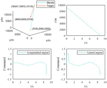
After determining the transition region, simulation verification is performed using the guidance law proposed in this paper. Since the actual guidance model cannot strictly follow the planned path and is affected by internal forces in the spatial environment, boundary points are avoided in the transition region during verification. Verification is completed by randomly selecting points in both the target region and the transition region. The initial parameter settings are shown in Table 2.

As shown in Fig. 7, arbitrary points selected from the calculated transition region and target region set can successfully complete the guidance control task. Although the missile acceleration was set as a constant value during planning, external force disturbances and the use of guidance laws instead of direct planning result in some deviation between the actual and planned paths. However, this does not affect its interceptability.

As depicted in Fig. 8(a), a comparison between the TMCC based on a compensator-observer and the traditional PN method indicates that TMCC has a shorter capture time and higher capture accuracy compared to the PN method. Figure 8(b) shows that a comparison between TMCC and PN trajectory control engine commands indicates that TMCC requires lower control input, thereby reducing energy consumption during the interception process. Use $\left| {\smallint {F_g}{\tau _g}dt} \right|$ to calculate the energy consumed.

Table 3.

Interception results

Figure 7.

Guidance simulation verification.

Figure 8.

Interception comparison chart.

It can be seen from Table 3 that TMCC has shorter intercept time and higher intercept accuracy than PN, because TMCC uses the acceleration information estimated by CFO to compensate the target acceleration into the controller, which uses more information than traditional PN and has higher accuracy. Compared with PN method, TMCC has smaller energy loss.

As there are certain requirements for the terminal guidance speed, there is a probability that interception may not be achievable. The following 6,000 groups are made to change the initial speed of the missile in the terminal guidance. Other parameter settings are the same as those in Table 2. If the miss distance is less than 1m, the interception will be considered successful, as shown in Fig. 9.

Figure 9.

Influence of interceptor initial velocity on interception.

Figure 9 shows the initial speed of the missile in three directions and the interception. Blue represents the success of interception, and red represents the miss distance greater than 1m. It can be clearly seen that the success rate of interception is very high in the range of $1,000\sim 1,600m/s$ and $1,000\sim 1,180m/s$ . The interception success rate is high at $3,000\sim 3,200m/s$ , and the interception accuracy is a little lower when the speed exceeds 3,200m/s. Among the 6,000 groups of simulations, only 268 groups missed more than 1m. The guidance method designed in this paper has a high success rate in this scenario.

6.0 Conclusion

This paper presents a three-dimensional target manoeuver compensation guidance law based on CFO and a method for calculating the midcourse-to-terminal handover region. An observer-based CFO is employed to estimate the target’s manoeuvering state and integrate this compensation into the guidance law. Additionally, a calculation method for the terminal guidance handover region is provided. When the target area is represented as a spherical shape, a conical-shaped handover region is derived. Finally, simulation validation is conducted in two parts. The first part involves simulating the midcourse-to-terminal handover region and validating it with the proposed guidance law, demonstrating that the computed handover region successfully completes the guidance control task. The second part compares the proposed guidance law with traditional proportional guidance. Due to the use of CFO to estimate the target’s motion information and feed it back into the controller, the TMCC interception accuracy is higher and energy loss is lower compared to the PN method.