1 Introduction
Central to biosphere–atmospheric exchanges, a scalar advected by a turbulent flow in the atmospheric surface layer, the so-called scalar turbulence, has been the subject of increasing research interest at the frontiers of different disciplines of the geosciences and the environmental sciences, including meteorology, climatology, hydrology, oceanography and ecology (Sreenivasan Reference Sreenivasan1991; Katul et al. Reference Katul, Cavac, Siqueria and Poggi2013). In particular, scalar turbulence at the vegetation canopy–atmosphere interface has attracted a great deal of attention in the past decades (Finnigan Reference Finnigan2000; Harman & Finnigan Reference Harman and Finnigan2008; Belcher, Harman & Finnigan Reference Belcher, Harman and Finnigan2012), as it explains heat and mass exchanges between the canopy and the above atmosphere.
Compared to surface boundary-layer flow, canopy flow (velocity) shows some similarities with a plane mixing-layer flow resulting from the interaction between a slower and a faster flow, within and above the canopy, respectively, where Kelvin–Helmholtz instabilities develop, reducing the flow anisotropy (Raupach, Finnigan & Brunet Reference Raupach, Finnigan and Brunet1996; Katul & Chang Reference Katul and Chang1999). Hence, canopy turbulence is a combination of mixing-layer-type coherent structures scaling with the vorticity thickness at the canopy top, surface-layer-type coherent structures whose length scales vary with distance from the surface and residual small wake eddies developing behind canopy elements (Poggi et al. Reference Poggi, Porporato, Ridolfi, Albertson and Katul2004; Dupont & Patton Reference Dupont and Patton2012). Near the canopy top, velocity fluctuations exhibit scale invariance from scales smaller than the mixing-layer-type coherent structures where turbulence is produced, to scales larger than the dissipation scale; while deeper within the canopy, this scale invariance is often weakened by the presence of specific-scale wake eddies developing behind canopy geometries with a dominant length scale such as a tree trunk diameter (Poggi et al. Reference Poggi, Porporato, Ridolfi, Albertson and Katul2004; Cava & Katul Reference Cava and Katul2008; Dupont et al. Reference Dupont, Irvine, Bonnefond, Lamaud and Brunet2012). With thermal instability, the canopy-top wind shear is weakened, and the shear-driven eddies are progressively replaced by buoyantly driven eddies in unstable conditions or damped in stable stratification (Dupont & Patton Reference Dupont and Patton2012).
Similar to scalar turbulence in common turbulent flows, the time series of active and passive scalar fields collected near the canopy top (e.g. temperature, particle or chemical species concentration, etc.) show both a larger intermittency at fine scales as compared to the longitudinal wind velocity (Schmitt et al. Reference Schmitt, Schertzer, Lovejoy and Brunet1996), and the ubiquitous presence of ramp–cliff patterns (Paw U et al. Reference Paw U, Brunet, Collineau, Shaw, Maitani, Qiu and Hipps1992; Katul et al. Reference Katul, Porporato, Cava and Siqueira2006, Reference Katul, Cavac, Siqueria and Poggi2013). The larger intermittency manifests itself by more intense and sporadic scalar fluctuations at small scales, leading statistically to a larger spectrum of singularities (multifractals), therefore contradicting the famous Kolmogorov (Kolmogorov Reference Kolmogorov1941)–Obukhov (Obukhov Reference Obukhov1949)–Corrsin (Corrsin Reference Corrsin1951) (KOC) universal scaling of scalar fluctuations at high moment order  $q$, i.e. for large fluctuations. The ramp–cliff patterns refer to gradual rises (respectively decreases) with weak scalar fluctuations over scales commensurate with the canopy height, followed by relatively sharp drops (respectively jumps) depending on whether the canopy is a source (respectively a sink) of the scalar under consideration. These structures have been the subject of intensive research due to their significant contribution to scalar turbulent fluxes (Gao, Shaw & Paw U Reference Gao, Shaw and Paw U1989; Katul et al. Reference Katul, Cavac, Siqueria and Poggi2013). Initially interpreted as the signature of convective plumes (Taylor Reference Taylor1958), these ramp–cliff patterns have been systematically observed from field and numerical experiments irrespective of the sign of the thermal stability, and whether the canopy is a source or a sink of the scalar (Gao et al. Reference Gao, Shaw and Paw U1989; Paw U et al. Reference Paw U, Brunet, Collineau, Shaw, Maitani, Qiu and Hipps1992; Fitzmaurice et al. Reference Fitzmaurice, Shaw, Paw U and Patton2004). These patterns appear related to the coherent structures developing at the canopy top, corresponding to the anisotropic forcing of scalar fluctuations. By analogy with the surface renewal theory (Higbie Reference Higbie1935), a ramp–cliff pattern observed in scalar time series is interpreted as the result of a parcel of fluid coming from the above bulk fluid that remains in contact with the canopy top where scalar sources (sinks) are located, increasing (decreasing) progressively the amount of scalar in the fluid parcel, before being replaced by another fluid parcel (Paw U et al. Reference Paw U, Qiu, Su, Watanabe and Brunet1995; Katul et al. Reference Katul, Porporato, Cava and Siqueira2006).
These ramp–cliff patterns are usually invoked as the possible cause of the larger fine-scale intermittency of scalar turbulence (Sreenivasan Reference Sreenivasan1991; Sreenivasan & Antonia Reference Sreenivasan and Antonia1997; Shraiman & Siggia Reference Shraiman and Siggia2000; Warhaft Reference Warhaft2000; Falkovich, Gawedzki & Vergassola Reference Falkovich, Gawedzki and Vergassola2001; Katul et al. Reference Katul, Angelini, De Canditiis, Amato, Vidakovic and Alberston2003; Zorzetto, Bragg & Katul Reference Zorzetto, Bragg and Katul2018), and thus the breakdown of the KOC scaling law of scalar fluctuations. Direct numerical simulations (Frisch, Mazzino & Vergassola Reference Frisch, Mazzino and Vergassola1998; Celani et al. Reference Celani, Lanotte, Mazzino and Vergassola2000; Celani, Mazzino & Vergassola Reference Celani, Mazzino and Vergassola2001; Iyer et al. Reference Iyer, Schumacher, Sreenivasan and Yeung2018) and laboratory experiments (Warhaft Reference Warhaft2000; Moisy et al. Reference Moisy, Willaime, Andersen and Tabeling2001) have further evidenced the role of cliff structures in saturating the scaling exponent of scalar fluctuations to a constant value for high moment order  $q$, the so-called phenomenon of intermittency saturation. Hence, conversely to the traditional picture of the scale by scale cascade of energy from the large-scale anisotropic forcing (integral scale) to the viscous dissipation scale, with a rapid loss of the forcing anisotropic character during the process, in the presence of ramp–cliff structures, it is often suggested that the cascading process may be short circuited with some coupling between large and small scales, the latter still carrying some signature from the forcing scale (Katul et al. Reference Katul, Angelini, De Canditiis, Amato, Vidakovic and Alberston2003; Zorzetto et al. Reference Zorzetto, Bragg and Katul2018).
Despite considerable theoretical (Lvov, Procaccia & Fairhall Reference Lvov, Procaccia and Fairhall1994; Chertkov Reference Chertkov1997; Pumir, Shraiman & Siggia Reference Pumir, Shraiman and Siggia1997; Yakhot Reference Yakhot1997; Balkovsky & Lebedev Reference Balkovsky and Lebedev1998; Falkovich et al. Reference Falkovich, Gawedzki and Vergassola2001), numerical (Meneveau, Lund & Cabot Reference Meneveau, Lund and Cabot1996; Higgins, Parlange & Meneveau Reference Higgins, Parlange and Meneveau2003; Watanabe & Gotoh Reference Watanabe and Gotoh2004; Xu et al. Reference Xu, Pumir, Falkovich, Bodenschatz, Shats, Xia, Francois and Boffetta2014) and experimental efforts (Sreenivasan Reference Sreenivasan1991; Frisch Reference Frisch1995; Sreenivasan & Antonia Reference Sreenivasan and Antonia1997; Pope Reference Pope2000; Warhaft Reference Warhaft2000; Moisy et al. Reference Moisy, Willaime, Andersen and Tabeling2001), some debate remains concerning the statistical contribution of the ramp–cliff structures to the scalar intermittency at fine scales. In particular, an important issue left open is, to which extent these coherent structures indeed contribute to the larger deviation from the KOC universal scaling of the structure function exponent of scalars compared to that of the longitudinal velocity, larger deviation indicating a more intermittent scalar bulk turbulence field. In other words, does the presence of ramp–cliff patterns in scalar signals explain the larger intermittency at fine scales of the scalar fluctuations compared to that of the longitudinal velocity fluctuations?
Here, the impact of ramp–cliff structures on the fine-scale intermittency of scalar fluctuations is experimentally investigated using a high-frequency air temperature ( $\unicode[STIX]{x1D703}$) measured at the top of a forest canopy for different thermal stratifications, and compared with the intermittency of the longitudinal velocity fluctuations (
 $u$) recorded at the same location. To that purpose, a multifractal analysis of the
 $\unicode[STIX]{x1D703}$ and
 $u$ signals is performed in order to characterize the scaling properties of
 $\unicode[STIX]{x1D703}$ and
 $u$ fluctuations according to the magnitude of the fluctuations (moment order), and to highlight the strength of the strongest singularities (cliff) across scales. The signal singularities are located using a wavelet transform and the statistical singularity strengths are deduced from the slopes of the local maxima of the wavelet transform modulus across scales using the wavelet transform modulus maxima (WTMM) method.
The structure of the paper is as follows. In § 2, the measurements and multifractal analysis are described. In § 3, the multifractal characteristics (scaling exponents, singularity spectra) of the air temperature ( $\unicode[STIX]{x1D703}$) and longitudinal velocity (
 $u$) at canopy top are compared for different stability regimes, with observation of the saturation of the scaling exponent of
 $\unicode[STIX]{x1D703}$ for high moment order and non-neutral conditions. Then, in § 4, we discuss this saturation behaviour in regards to the presence of cliff singularities in the signal, suggesting an analogy with an ordered–disordered phase transition at a critical moment order, where the ordered phase is dominated by ‘cliff’ singularities and the disordered phase by a large spectrum of singularity strengths. The absence of saturation in near-neutral conditions while
 $\unicode[STIX]{x1D703}$ fluctuations are still more intermittent than
 $u$ fluctuations leads us to conclude that the statistical contribution of the ‘cliffs’ is not significant enough to explain the stronger intermittency of
 $\unicode[STIX]{x1D703}$ fluctuations. Finally, in § 5 the outcomes of the study are summarized and concluding remarks presented.
2 Material and method
2.1 Measurements
The air temperature and the three wind velocity components were measured during the summer 2016 within the atmospheric surface layer, near the top of a maritime pine forest ( $z=9.85~\text{m}$), using a three-dimensional sonic anemometer (Gill R3) sampling at 20 Hz. The forest plot was located at the Salles Integrated Carbon Observation Station (ICOS) (
 $44^{\circ }29^{\prime }~\text{N}$,
 $0^{\circ }57^{\prime }~\text{W}$), in Les Landes region, in southwestern France. The forest was characterized by a mean tree height of
 $h=8.4~\text{m}$ and a leaf area index of approximately 3.2. This latter parameter indicates a canopy sufficiently dense to induce a mixing-layer-type flow at its top. The ground surface was flat in all directions, and the forest was wide enough to have negligible fetch effect in all wind directions. The recorded wind velocity components were rotated horizontally so that the longitudinal velocity (
 $u$) represents the horizontal component along the mean wind direction. To account for a possible error in the vertical orientation of the sonic anemometer, a second rotation was performed around the transverse axis to ensure a zero mean vertical velocity (
 $w$). The air temperature (
 $\unicode[STIX]{x1D703}$) was deduced from the sonic anemometer speed of sound.
Following standard quality controls, a total of 27 time series (runs), of 217 data points each (∼109 min), were selected for both  $\unicode[STIX]{x1D703}$ and
 $u$. These runs covered different thermal stratifications, also referred to as stability regimes, ranging from unstable, near neutral to stable conditions, where the stability was defined from the stability parameter
 $\unicode[STIX]{x1D701}=z/L$ at the canopy top, as commonly used in atmospheric surface-layer studies. Here,
 $L$ is the Obukhov length (Obukhov Reference Obukhov1946) defined as
 $L=-u_{\ast }^{3}T/(\unicode[STIX]{x1D705}g\overline{w^{\prime }T^{\prime }})$, where
 $u_{\ast }$ is the friction velocity characterizing the momentum absorbed by the vegetated surface,
 $T$ is the air temperature,
 $g$ the gravitational acceleration and
 $\overline{w^{\prime }T^{\prime }}$ the kinematic sensible heat flux;
 $L$ characterizes the height above which buoyant production (or destruction) of turbulent kinetic energy dominates the mechanical production. The sign of
 $L$ reflects the direction of the heat flux, positive for daily unstable conditions with an upward heat flux, and negative for nocturnal stable conditions with a downward heat flux. In near-neutral conditions, the thermal stratification of the atmosphere is negligible and
 $|L|\rightarrow \infty$, leading to
 $|\unicode[STIX]{x1D701}|\rightarrow 0$. For the range of stability conditions considered here, the mechanical production of turbulence is expected to always dominate the buoyant production or destruction.
To both investigate high-order moments and preserve turbulence stationarity, a time series length compromise of ∼109 min was reached. The time series included approximately 200 to 1400 integral scales of  $u$ and
 $\unicode[STIX]{x1D703}$ (
 $L_{u}$ and
 $L_{\unicode[STIX]{x1D703}}$, respectively) and 2300 to 7000 integral scales of
 $w$ (
 $L_{w}$), varying with the stability. The wavelet transform of the signals was performed with the third derivative of the Gaussian wavelet, as described further, to remove the signal large-scale trends (third-order polynomial trends). To further ensure the similarity of turbulent eddies along the time series and their stationarity, we only kept those with a small variability of
 $\unicode[STIX]{x1D701}$. Unstable and stable runs were also selected under clear sky conditions and at the same time during the day, around midday and early night, respectively, to keep close radiation forcing and atmospheric boundary-layer conditions for runs of the same stability.
The Taylor hypothesis of frozen turbulence is usually applied to local point measurements to convert temporal to spatial scales (Kaimal & Finnigan Reference Kaimal and Finnigan1994), assuming that velocity fluctuations are much smaller than the mean velocity of the main eddies ( $U_{c}$), i.e.
 $\unicode[STIX]{x1D70E}_{u}^{2}/U_{c}^{2}<<1$ with
 $\unicode[STIX]{x1D70E}_{u}$ the standard deviation of the longitudinal velocity (Lin Reference Lin1953). Even if the well-known mixing-layer-type flow prevailing at the canopy top leads to velocity fluctuations of the same order as the mean wind velocity (
 $U_{h}$), the mean convection velocity of the main eddies (
 $U_{c}$) is larger than
 $U_{h}$,
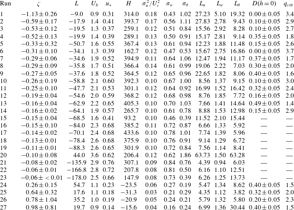
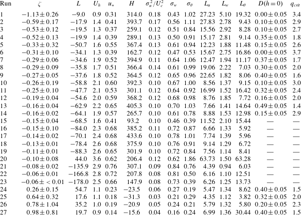
 $U_{c}\approx 1.8\;U_{h}$ (Raupach et al. Reference Raupach, Finnigan and Brunet1996), which extends the validity the Taylor hypothesis at the canopy top (Kaimal & Finnigan Reference Kaimal and Finnigan1994). The squared turbulence intensity relative to the squared convection velocity varies from 0.04 in stable conditions up to 0.18 for the most unstable runs (table 1), reaching the limit of applicability of the Taylor hypothesis for these latter runs. To overcome this limitation, we normalized the time scale with
 $L_{w}$ (the integral scale of the vertical velocity
 $w$) (Zorzetto et al. Reference Zorzetto, Bragg and Katul2018), assuming that the distortion of the main advected eddies impacted similarly the time scale and
 $L_{w}$,
 $L_{w}$ being much smaller than
 $L_{u}$ (table 1).
Main characteristics of the selected runs: the atmospheric stability parameter  $\unicode[STIX]{x1D701}$, the Obukhov length
 $L$ (m), the mean wind speed at canopy top
 $U_{h}$ (
 $\text{m}~\text{s}^{-1}$), the friction velocity
 $u_{\ast }$ (
 $\text{m}~\text{s}^{-1}$), the sensible heat flux (
 $\text{W}~\text{m}^{-2}$), the turbulent intensity
 $\unicode[STIX]{x1D70E}_{u}/U_{c}$ (where
 $\unicode[STIX]{x1D70E}_{u}$ is the standard deviation of the longitudinal velocity and
 $U_{c}$ the eddy convection velocity), the vertical velocity standard deviation
 $\unicode[STIX]{x1D70E}_{w}$ (
 $\text{m}~\text{s}^{-1}$), the air temperature standard deviation
 $\unicode[STIX]{x1D70E}_{\unicode[STIX]{x1D703}}$ (K), the integral time scale of the longitudinal velocity
 $L_{u}$ (s), the integral time scale of the vertical velocity
 $L_{w}$ (s), the integral time scale of the air temperature
 $L_{\unicode[STIX]{x1D703}}$ (s), the fractal dimension of the strong cliff singularities (
 $D(h=0)$) and the critical value of
 $q$ at the phase transition (
 $q_{crit}$).
The ratio between the integral scales of  $u$ and
 $w$ (
 $L_{u}/L_{w}$) is approximately 7.5, exhibiting the anisotropy of the large-scale wind motions at the canopy top, and is intermediate between the expected values in surface-layer and mixing-layer flows (Katul & Chang Reference Katul and Chang1999). This value of 7.5 is close to the ratio observed by Katul & Chang (Reference Katul and Chang1999) for a pine forest, showing the generality of our canopy flow.
2.2 Multifractal analysis
The WTMM method was used to perform the multifractal analysis. This method has proved very efficient in estimating scaling exponents and singularity spectra of complex non-stationary time series related to various research areas, including fully developed turbulence (Muzy, Bacry & Arneodo Reference Muzy, Bacry and Arneodo1994; Arneodo, Manneville & Muzy Reference Arneodo, Manneville and Muzy1998c; Arneodo, Muzy & Sornette Reference Arneodo, Muzy and Sornette1998d; Delour, Muzy & Arneodo Reference Delour, Muzy and Arneodo2001; Arneodo et al. Reference Arneodo, Audit, Decoster, Muzy and Vaillant2002; Audit et al. Reference Audit, Bacry, Muzy and Arneodo2002; Arneodo et al. Reference Arneodo, Decoster, Kestener and Roux2003; Khalil et al. Reference Khalil, Joncas, Nekka, Kestener and Arneodo2006; Arneodo et al. Reference Arneodo, Audit, Kestener and Roux2008; Roland et al. Reference Roland, Khalil, Tanenbaum, Berguiga, Delichere, Bonneviot, Elezgaray, Arneodo and Argoul2009; Roux et al. Reference Roux, Venugopal, Fienberg, Arneodo and Foufoula-Georgiou2009; Arneodo et al. Reference Arneodo, Vaillant, Audit, Argoul, d’Aubenton Carafa and Thermes2011). Compared to the structure function method, the WTMM method allows one to extract the entire range of non-oscillating singularities (cusp type) present in the signal provided that the wavelet is sufficiently smooth and localized in time and frequency, and with a sufficient number of vanishing moments (Muzy, Bacry & Arneodo Reference Muzy, Bacry and Arneodo1993). Oscillating singularities (chirp type) are not expected or are negligible in our turbulence data as confirmed by Lashermes et al. (Reference Lashermes, Roux, Abry and Jaffard2008) and Abry, Roux & Jaffard (Reference Abry, Roux and Jaffard2011) on wind-tunnel turbulence data.
The strengths of the singularities of the wind velocity and air temperature signals  $f$ were computed from their wavelet transform (WT). The WT can be compared to a mathematical microscope (Muzy, Bacry & Arneodo Reference Muzy, Bacry and Arneodo1991; Muzy et al. Reference Muzy, Bacry and Arneodo1994; Arneodo, Bacry & Muzy Reference Arneodo, Bacry and Muzy1995) whose lenses are a family of wavelets
 $\unicode[STIX]{x1D713}$ with different zooming factors, characterized by the scale parameter
 $a$, which are shifted along the signal with a translation parameter
 $b$. The WT is well suited for the analysis of complex non-stationary time series such as those found in the atmosphere. The continuous wavelet transform of the function
 $f(t)$ is defined as
 $$\begin{eqnarray}T_{\unicode[STIX]{x1D713}}[f](b,a)={\displaystyle \frac{1}{|a|}}\int f(t)\overline{\unicode[STIX]{x1D713}}\left({\displaystyle \frac{t-b}{a}}\right)\,\text{d}t,\end{eqnarray}$$
where  $f$ is here either
 $u$ or
 $\unicode[STIX]{x1D703}$,
 $T_{\unicode[STIX]{x1D713}}[f](b,a)$ is the wavelet coefficient that characterizes the degree of correlation between the signal
 $f$ and the wavelet at the location
 $b$ and for the wavelet scale
 $a$;
 $\overline{\unicode[STIX]{x1D713}}$ denotes the complex conjugate of
 $\unicode[STIX]{x1D713}$. In our study, a third derivative of the Gaussian function was chosen as the wavelet (in which case the complex conjugate of
 $\unicode[STIX]{x1D713}$ identifies to
 $\unicode[STIX]{x1D713}$). This wavelet is well localized in both space and frequency and is well suited to detecting discontinuities like cliffs in signals, as demonstrated by its extensive use with geophysical or medical signals (e.g. Muzy et al. Reference Muzy, Bacry and Arneodo1994; Arneodo et al. Reference Arneodo, Bacry and Muzy1995; Venugopal et al. Reference Venugopal, Roux, Foufoula-Georgiou and Arneodo2006; Gerasimova et al. Reference Gerasimova, Audit, Roux, Khalil, Gileva, Argoul, Naimark and Arneodo2014; Attuel et al. Reference Attuel, Gerasimova-Chechkina, Argoul, Yahia and Arneodo2018). More importantly, this wavelet allows us to remove polynomial trends of order less than or equal to three from the function
 $f(t)$, which is important when dealing with long meteorological time series.
The singularities of the signal  $f$ are then localized from the maximum lines of the wavelet transform modulus
 $|T_{\unicode[STIX]{x1D713}}[f](t,a)|$ of
 $f$, connected across scales
 $a$ at time
 $t$ as
 $a\rightarrow 0^{+}$. The strength of these singularities, also called local Hölder exponents
 $h(t)$ (Mallat & Hwang Reference Mallat and Hwang1992), are precisely the scaling exponents of the WTMM line pointing at the singularity. These lines define the wavelet transform skeleton
 ${\mathcal{L}}(a)$.
Under the canonical multifractal formalism, the distribution of  $h$ values given by the singularity spectrum
 $D(h)$ characterizes the set of singularities, and hence the fractal properties of the signal;
 $D(h)$ is computed through a Legendre transformation (2.2) of the scaling exponent
 $\unicode[STIX]{x1D70F}(q)$ of the partition functions
 $Z(q,a)$ (2.3) restricted to the subset of points of the WTMM skeleton
 ${\mathcal{L}}(a)$ at each scale
 $a$
 $$\begin{eqnarray}\displaystyle & \displaystyle D(h)=\min _{q}[qh-\unicode[STIX]{x1D70F}(q)], & \displaystyle\end{eqnarray}$$
 $$\begin{eqnarray}\displaystyle & \displaystyle Z(q,a)=\mathop{\sum }_{l\in {\mathcal{L}}(a)}\left[\sup _{(t,a^{\prime })\in l,a^{\prime }\leqslant a}|T_{\unicode[STIX]{x1D713}}[f](t,a^{\prime })|\right]^{q}\sim a^{\unicode[STIX]{x1D70F}(q)}, & \displaystyle\end{eqnarray}$$
where  $q\in \mathbb{R}$ is the moment order. To avoid numerical instabilities inherent to the Legendre transform, the expectation values
 $h(q,a)=\unicode[STIX]{x2202}[\ln (Z(q,a))]/\unicode[STIX]{x2202}q$ and
 $D(q,a)=q\unicode[STIX]{x2202}[\ln (Z(q,a))]/\unicode[STIX]{x2202}q-\ln (Z(q,a))$ were computed first (Arneodo et al. Reference Arneodo, Bacry and Muzy1995). Then, the slopes of
 $h(q,a)$ and
 $D(q,a)$ versus
 $\ln a$ gave
 $h(q)$ and
 $D(q)$, and therefore the
 $D(h)$ singularity spectrum as a curve parametrized by
 $q$.
The maximum moment order  $q$ chosen in our analysis was based on (i) the convergence of the moments of the wavelet coefficients along the time series for scales within the scaling regime, and (ii) the quality of the scaling of the partition function
 $\log _{2}(Z(q,a))$ versus the normalized scale
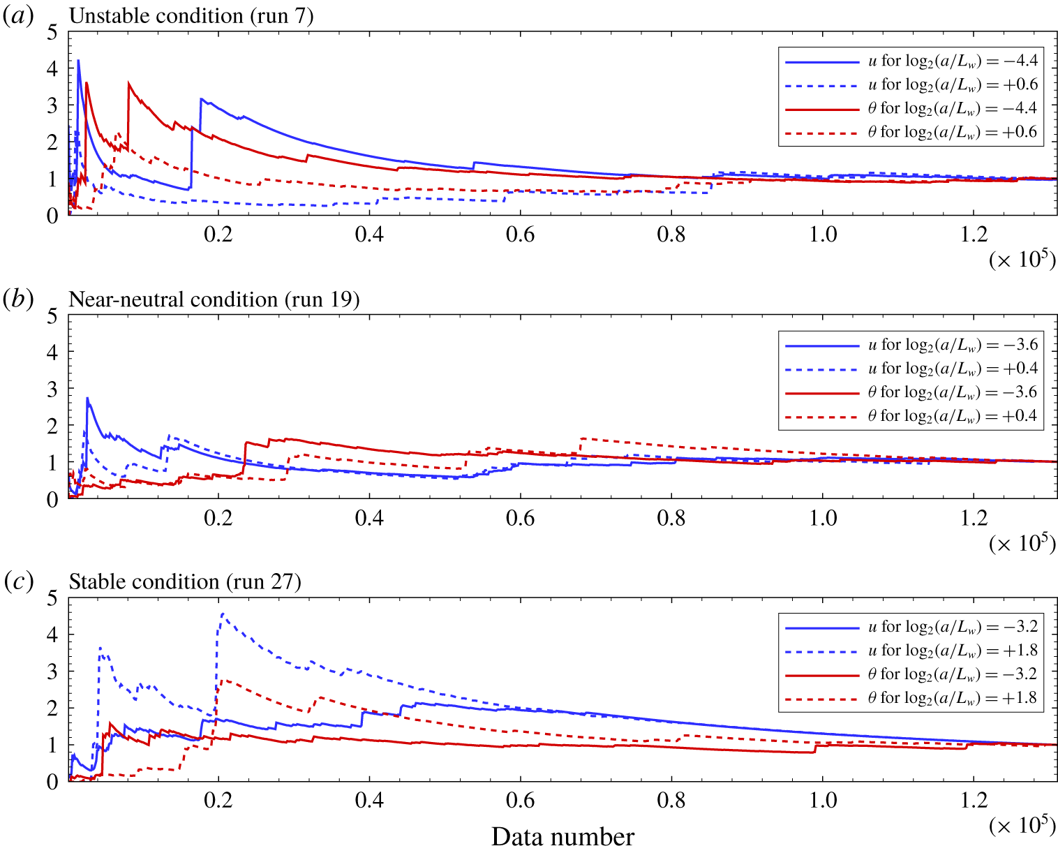
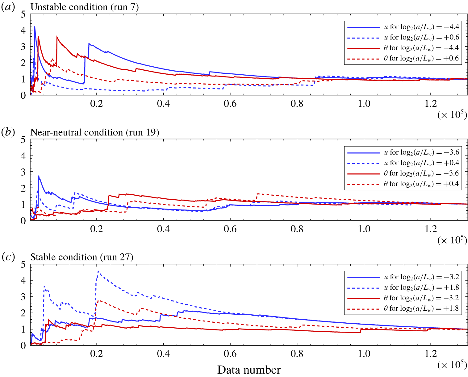
 $\log _{2}(a/L_{w})$. Figure 1 shows an example of convergence with time of the moment of order 6 of the
 $u$ and
 $\unicode[STIX]{x1D703}$ wavelet coefficients at two scales delimiting the scaling regime, for an unstable, near neutral and stable run. The convergence appears relatively well attained during the last 10 % of the time series, with variations lower than ±10 % of the final value. This accuracy validation of the choice of the moment order is similar to the convergence method proposed by Anselmet et al. (Reference Anselmet, Gagne, Hopfinger and Antonia1984). Analysing the scaling of the partition functions for moment order
 $q$ up to 8 demonstrated that the range of scales for a valid estimation of the scaling exponent was drastically shortened for
 $q$ larger than 6. The maximum moment order
 $q$ was fixed to 6.
Convergence with time of the moment order 6 of the  $u$ and
 $\unicode[STIX]{x1D703}$ wavelet coefficients at two scales delimiting the scaling regime, for an unstable (a), near neutral (b) and stable (c) run.
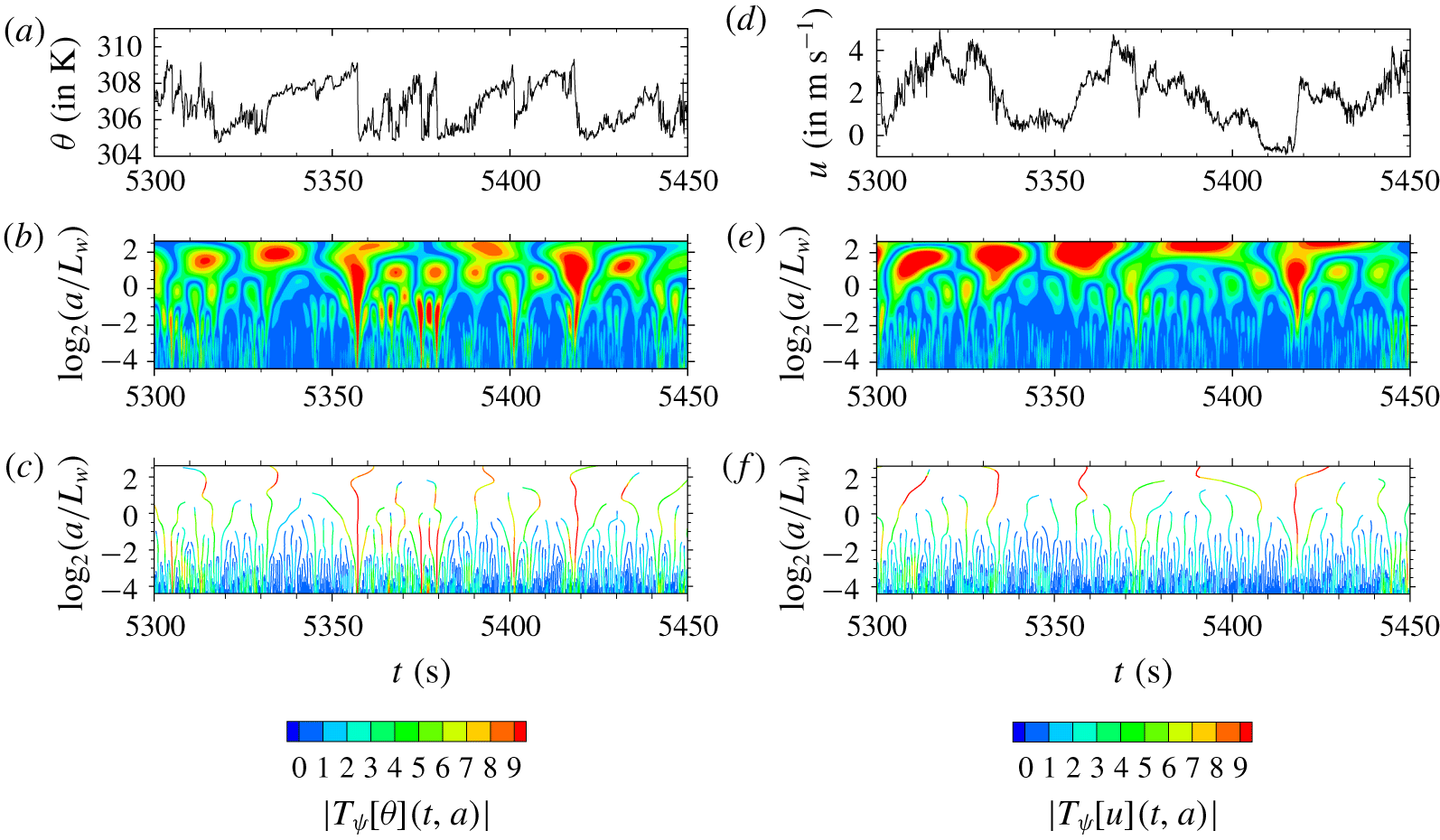
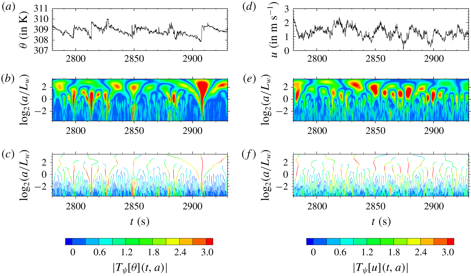
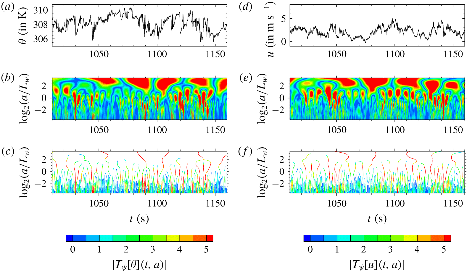
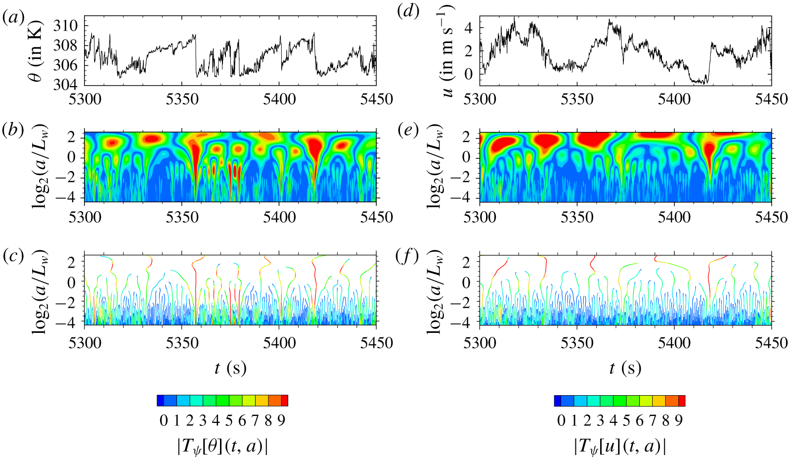
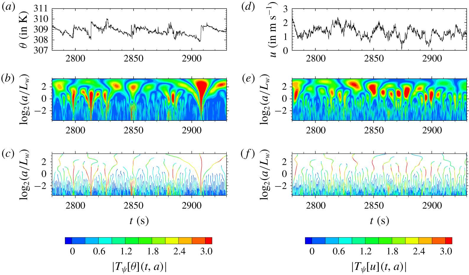
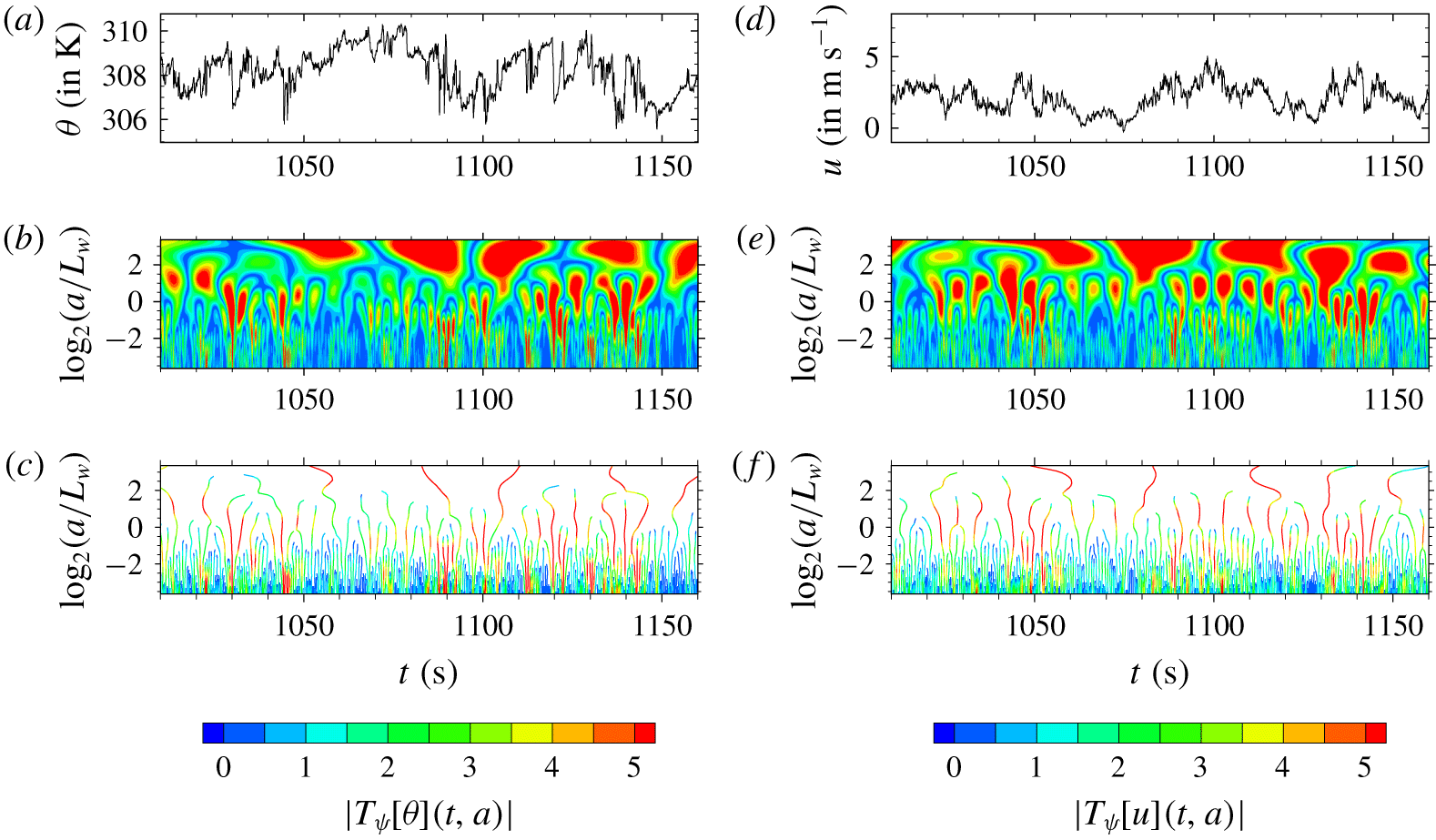
Finally, figures 2 to 4 illustrate the wavelet transform analysis of portions of the  $\unicode[STIX]{x1D703}$ and
 $u$ time series at the top of the canopy for an unstable, a near neutral and a stable case, runs 7, 19 and 27, respectively. Unlike the
 $u$ signal, the
 $\unicode[STIX]{x1D703}$ signal exhibits ramp–cliff structures in non-neutral cases. In the unstable case, these structures correspond to gradual rise of air temperature with weak scalar fluctuations over scales commensurate with the integral scale, followed by a relatively sharp drop. As expected, in the stable case, these ramp–cliff patterns in the
 $\unicode[STIX]{x1D703}$ signal are inverted due to the inversion of the temperature vertical gradient. In the near-neutral case, the ramp–cliff structures are not as well defined for this transitional regime between uprising and decreasing ramps. The maximum lines of the wavelet transform modulus define the wavelet transform skeleton (figures 2–4c). The cliff singularities appear on the wavelet transform modulus as cone-like structures pointing toward the signal discontinuities or singularities at the smallest scales, while the ramp structures give a smaller and smoother wavelet transform modulus (weaker singularities) (figures 2–4b). The strongest cliff singularities visible on the non-neutral cases have the longest maximum lines, crossing all scales, with a slow decrease of the modulus
 $|T_{\unicode[STIX]{x1D713}}[\unicode[STIX]{x1D703}](t,a)|$ along their maximum lines as
 $a\rightarrow 0^{+}$, leading to near-zero Hölder exponents. Interestingly, the time-scale distributions of the wavelet transform modulus of both the
 $\unicode[STIX]{x1D703}$ and
 $u$ signals show some branching structures, starting from large scales where eddies divide asymmetrically into smaller ones, and so on, as depicted in figures 2(b–e) and 3(b–e) through the imbrication of cone-like structures related to abrupt changes in the signals at different scales. This hierarchical distribution of the wavelet transform modulus is similar to the branching structure obtained from a non-homogeneous Cantor set, resulting from deterministic hierarchical construction rules (see figure 1 in Argoul et al. (Reference Argoul, Arneodo, Grasseau, Gagne, Hopfinger and Frisch1989)). This represents a visual evidence that the singularities appear hierarchically distributed on a ‘Cantor-like’ set, suggesting the presence of a multiplicative cascading process, as previously reported by Argoul et al. (Reference Argoul, Arneodo, Grasseau, Gagne, Hopfinger and Frisch1989) from a velocity field of wind-tunnel turbulence at very high Reynolds numbers.
Wavelet transform analysis of an air temperature time series ( $\unicode[STIX]{x1D703}(t)$) and a longitudinal wind velocity time series (
 $u(t)$) of length
 ${\sim}24$ integral scales, measured at the canopy top in an unstable atmospheric regime (run 7 in table 1). (a,d)
 $\unicode[STIX]{x1D703}$ and
 $u$ time series on a 150 s interval, the ramp–cliff patterns are visible in
 $\unicode[STIX]{x1D703}(t)$. (b,e) Moduli
 $|T_{\unicode[STIX]{x1D713}}[\unicode[STIX]{x1D703}](t,a)|$ and
 $|T_{\unicode[STIX]{x1D713}}[u](t,a)|$ of the wavelet transforms of
 $\unicode[STIX]{x1D703}(t)$ and
 $u(t)$, respectively. (c,f) Wavelet transform skeleton defined by the WTMM lines. The colour of the maximum lines corresponds to
 $|T_{\unicode[STIX]{x1D713}}|$. Panels (b,c,e,f) have the same colour map coding. The scale
 $a$ is normalized by the integral scale of the vertical velocity (
 $L_{w}$).


3 Results
3.1 Multifractal characteristics of  $\unicode[STIX]{x1D703}$ and $u$


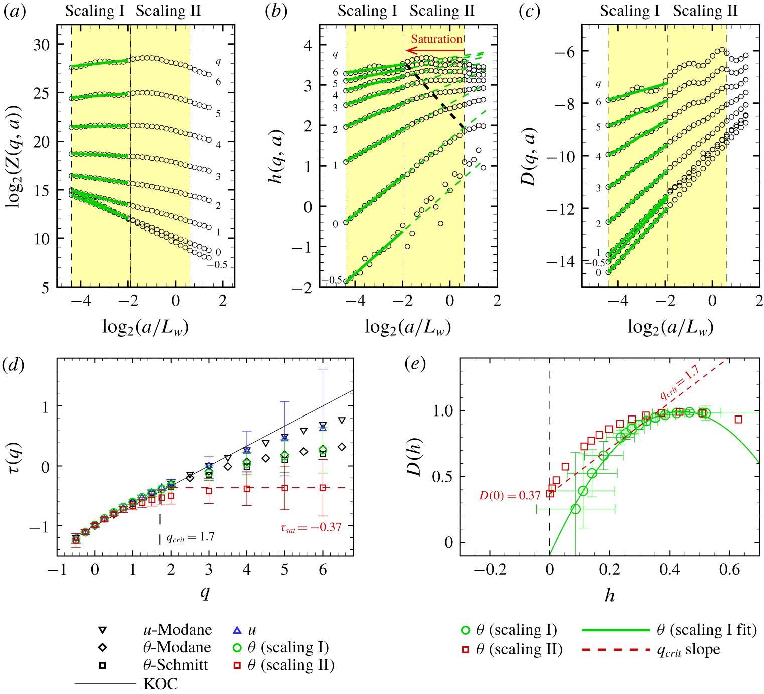
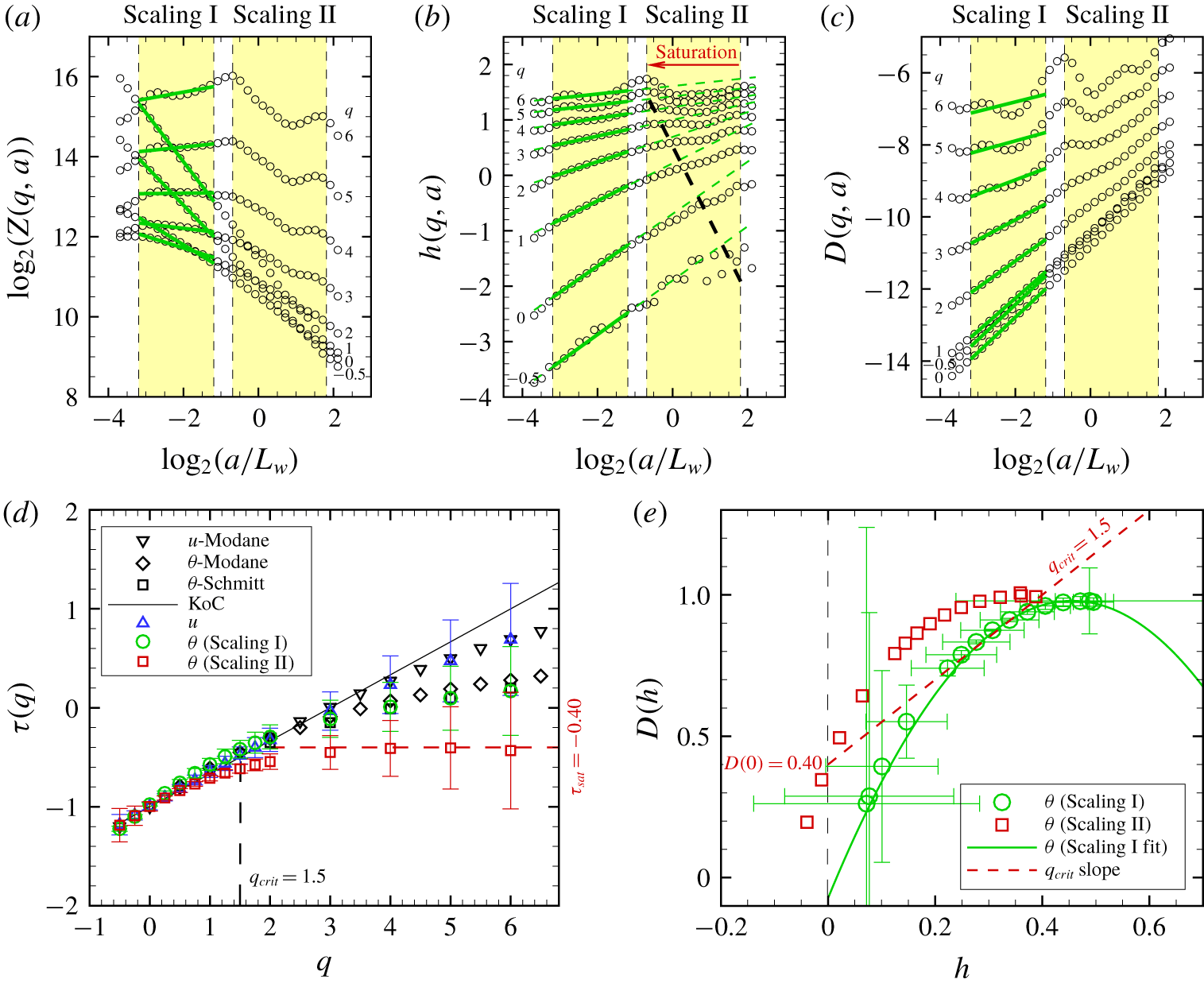
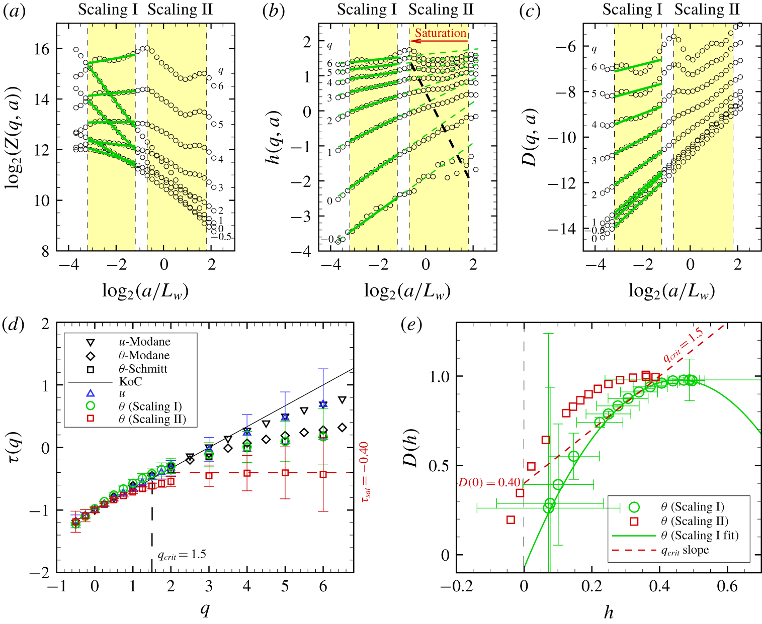
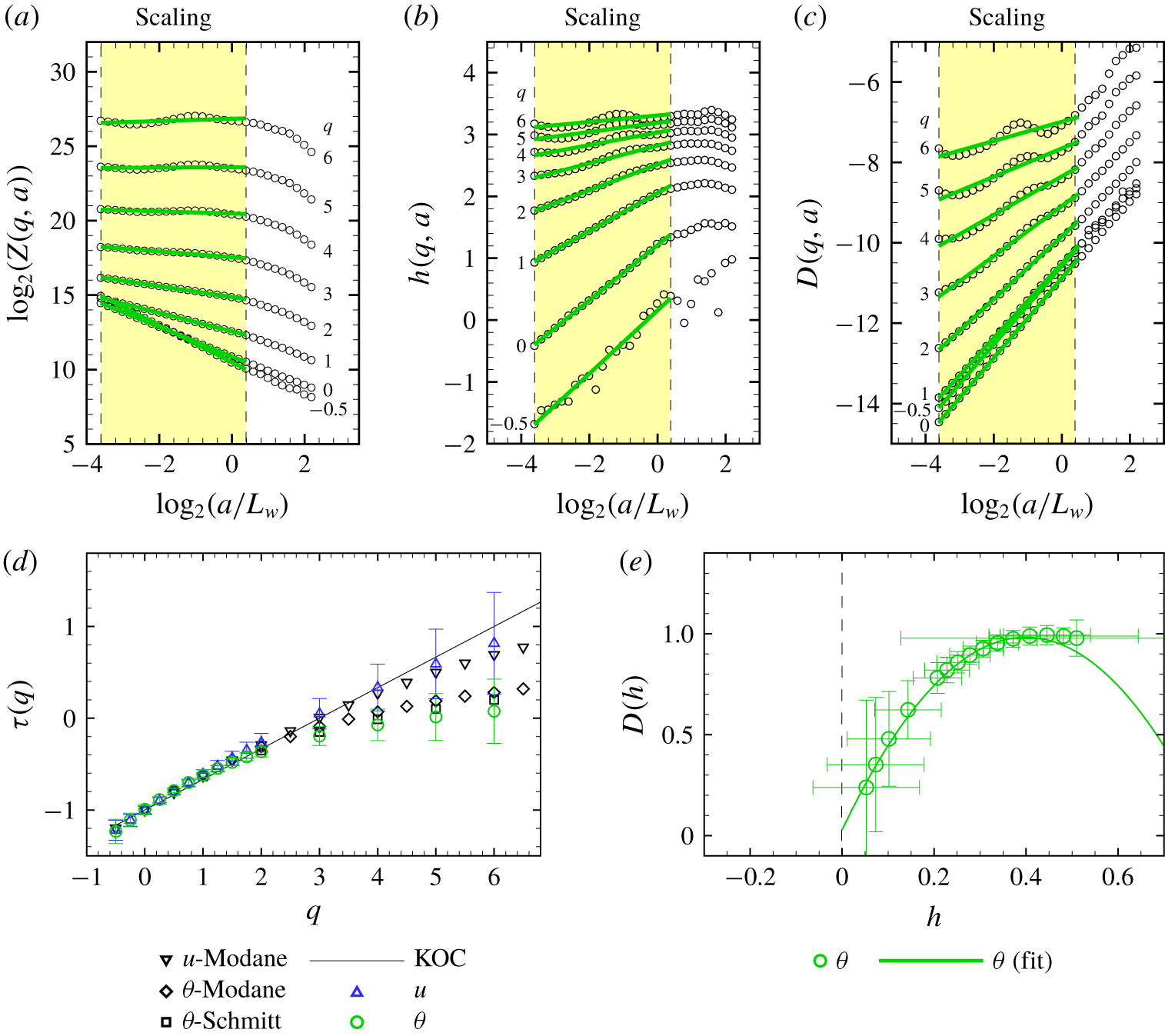
The WTMM analysis of the air temperature time series is illustrated in figure 5 for the unstable run 7. It reveals two scaling regimes over two successive ranges of scales within the inertial convective subrange ( $a<L_{\unicode[STIX]{x1D703}}$), for
 $q=-0.5$ to 6 (figure 5a–c). This is visible from the log–log plot of the partition function
 $Z(q,a)$ as a function of the scale
 $a$. The first scaling regime occurs at scales smaller than
 $L_{w}$, while the second scaling regime extends up to
 $L_{w}$. Hereafter, these regimes are referred to as scaling I and II.
Multifractal analysis of the canopy-top air temperature under an unstable atmospheric regime (run 7 in table 1) using the WTMM method. (a) Partition function  $\log _{2}(Z(q,a))$ versus
 $\log _{2}(a/L_{w})$. (b)
 $\log _{2}(h(q,a))$ versus
 $\log _{2}(a/L_{w})$. The black dashed line delimits the progressive invaded scaling regime II toward smaller scales with increasing
 $q$. (c)
 $\log _{2}(D(q,a))$ versus
 $\log _{2}(a/L_{w})$. (d) The scaling functions
 $\unicode[STIX]{x1D70F}(q)$ versus the moment order
 $q$ estimated by linear regression fit of
 $\log _{2}(Z(q,a))$ versus
 $\log _{2}(a)$ for both scaling regions, and compared with
 $\unicode[STIX]{x1D70F}(q)$ of the isotropic–homogeneous turbulent flows of Modane, compiled experiments (Schmitt Reference Schmitt2005) and prediction from KOC turbulence theory. The scaling function
 $\unicode[STIX]{x1D70F}(q)$ obtained for the longitudinal wind velocity (
 $u$) is also presented and compared with the Modane values. (e) The singularity spectra
 $D(h)$ versus the singularity strength
 $h$ obtained from linear regression fits of
 $\log _{2}(h(q,a))$ and
 $\log _{2}(D(q,a))$ versus
 $\log _{2}(a)$. The red dashed line represents the linear extension of
 $D_{II}(h)$ fall off towards + 0. 37 for
 $h=0$ (
 $D_{II}(h=0)=-\unicode[STIX]{x1D70F}_{sat}$) with a slope equal to
 $q_{crit}$. For clarity, error bars on
 $D(h)$ are partially represented. In (a–c), the two yellow boxes delimit the two scaling regimes I and II. The green solid lines represent the linear fit for the scaling regime I. The dashed green lines in (b) extend the linear fit obtained for the scaling regime I into the scaling regime II to highlight the saturation propagation due to ‘cliff’ singularities with decreasing scale and increasing
 $q$.
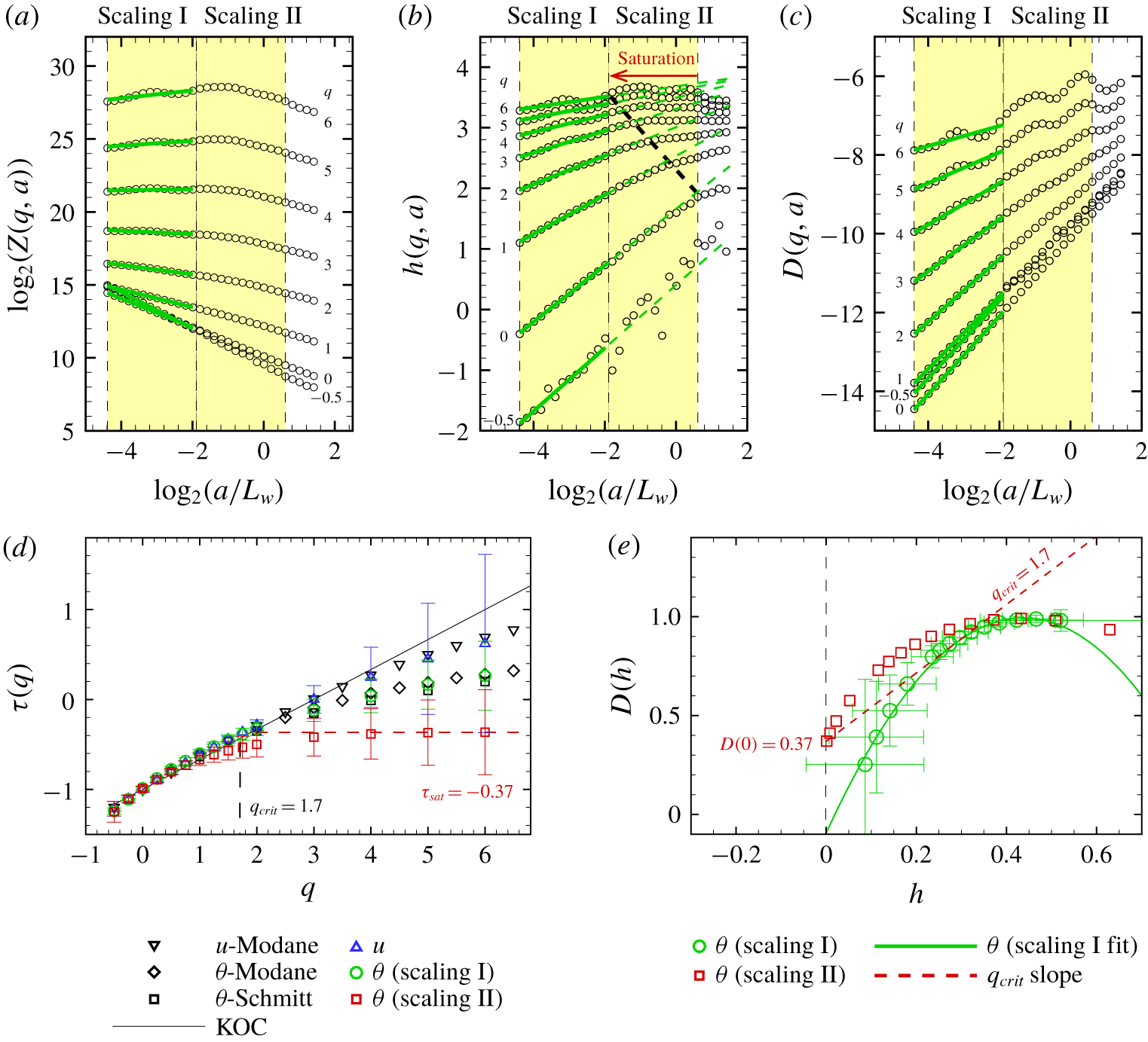
The scaling exponent  $\unicode[STIX]{x1D70F}_{I}(q)$ obtained for the scaling regime I from the linear regression fit of
 $\log _{2}(Z(q,a))$ versus
 $\log _{2}(a)$, has a nonlinear convex increasing form. This form is well approximated by a quadratic spectrum
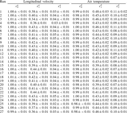
 $\unicode[STIX]{x1D70F}_{I}(q)=-c_{0}^{\unicode[STIX]{x1D703}}+c_{1}^{\unicode[STIX]{x1D703}}q-c_{2}^{\unicode[STIX]{x1D703}}q^{2}/2!$ (figure 5d), where
 $c_{0}^{\unicode[STIX]{x1D703}}$,
 $c_{1}^{\unicode[STIX]{x1D703}}$, and
 $c_{2}^{\unicode[STIX]{x1D703}}$ are fitting coefficients (table 2). This spectrum
 $\unicode[STIX]{x1D70F}_{I}(q)$ fits well with that obtained for temperature in homogeneous and isotropic flows of the Modane wind tunnel and other experiments (Schmitt Reference Schmitt2005). The nonlinear form of
 $\unicode[STIX]{x1D70F}_{I}(q)$ is corroborated by the dependence of the scaling behaviour of
 $h(q,a)$ versus
 $q$, suggesting a range of singularity exponents (
 $h$) in the signal. Hence, the singularity spectrum
 $D_{I}(h)$ exhibits a single humped shape over a finite range of Hölder exponents, varying from
 $h_{min}=0.1$ to
 $h_{max}=0.5$ for
 $q$ decreasing from 6 to - 0. 5 (figure 5e). This represents the signature of the multifractality of the temporal fluctuations of
 $\unicode[STIX]{x1D703}(t)$.
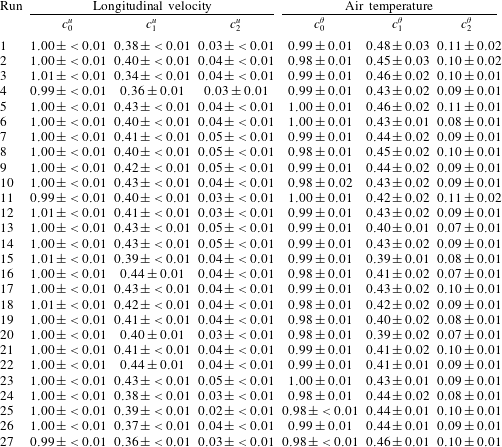
Coefficients  $c_{0}$,
 $c_{1}$ and
 $c_{2}$ of the polynomial expansion of
 $\unicode[STIX]{x1D70F}(q)$ (
 $\unicode[STIX]{x1D70F}(q)=-c_{0}+c_{1}q-c_{2}q^{2}/2!$) obtained from the WTMM multifractal analysis of the longitudinal velocity
 $u$ and air temperature
 $\unicode[STIX]{x1D703}$ (scaling I), for the 27 selected runs (table 1).
The scaling regime II exhibits a saturation of  $\unicode[STIX]{x1D70F}_{II}(q)$ for high
 $q$ values:
 $\unicode[STIX]{x1D70F}_{sat}\sim -0.37$ (figure 5d). Interestingly,
 $\unicode[STIX]{x1D70F}_{II}(q)$ and
 $D_{II}(h)$ spectra are similar to
 $\unicode[STIX]{x1D70F}_{I}(q)$ and
 $D_{I}(h)$ spectra for low
 $q$ values, respectively (figure 5d–e). Looking closer, the slopes of
 $\log _{2}(Z_{II}(q,a))$,
 $h_{II}(q,a)$ and
 $D_{II}(q,a)$ versus
 $\log _{2}(a/L_{w})$ at low
 $q$ values appear as the continuation of the slopes of the scaling regime I (figure 5a–c). Interestingly, the cross-over of
 $h(q,a)$ between the scaling regimes I and II evolves with
 $q$, the slope of
 $h(q,a)$ decreases from the larger scale of the scaling regime II, and invades progressively the smaller scales with increasing
 $q$, reflecting the dominance of strong singularities (
 $h=0$) for high
 $q$ values (figure 5b). These strong singularities are the signature of the cliff patterns observed in figure 2. Concomitantly,
 $D_{II}(h)$ extends toward smaller
 $h$ than
 $D_{I}(h)$ as the strong cliff singularities become statistically significant for this scale range.
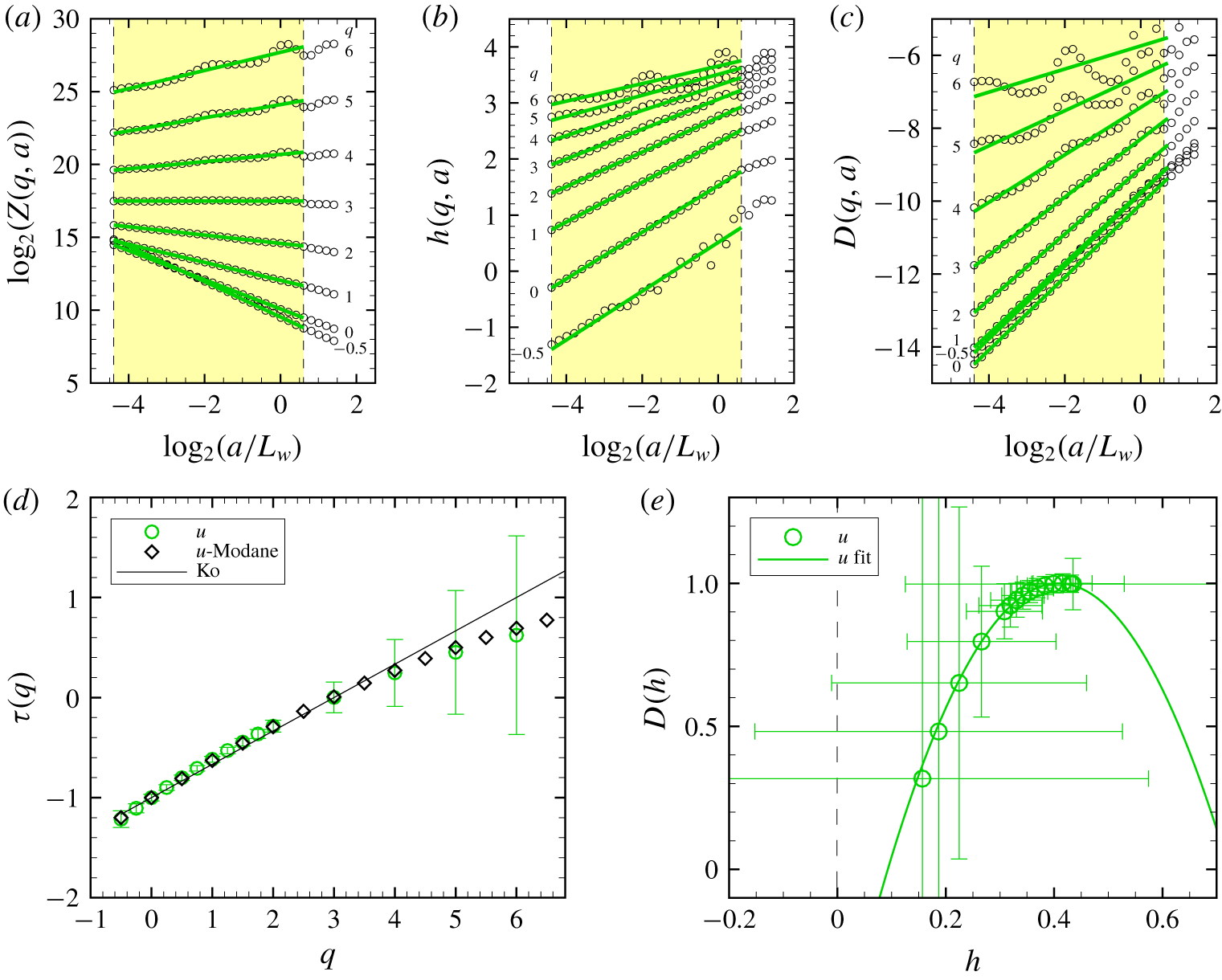
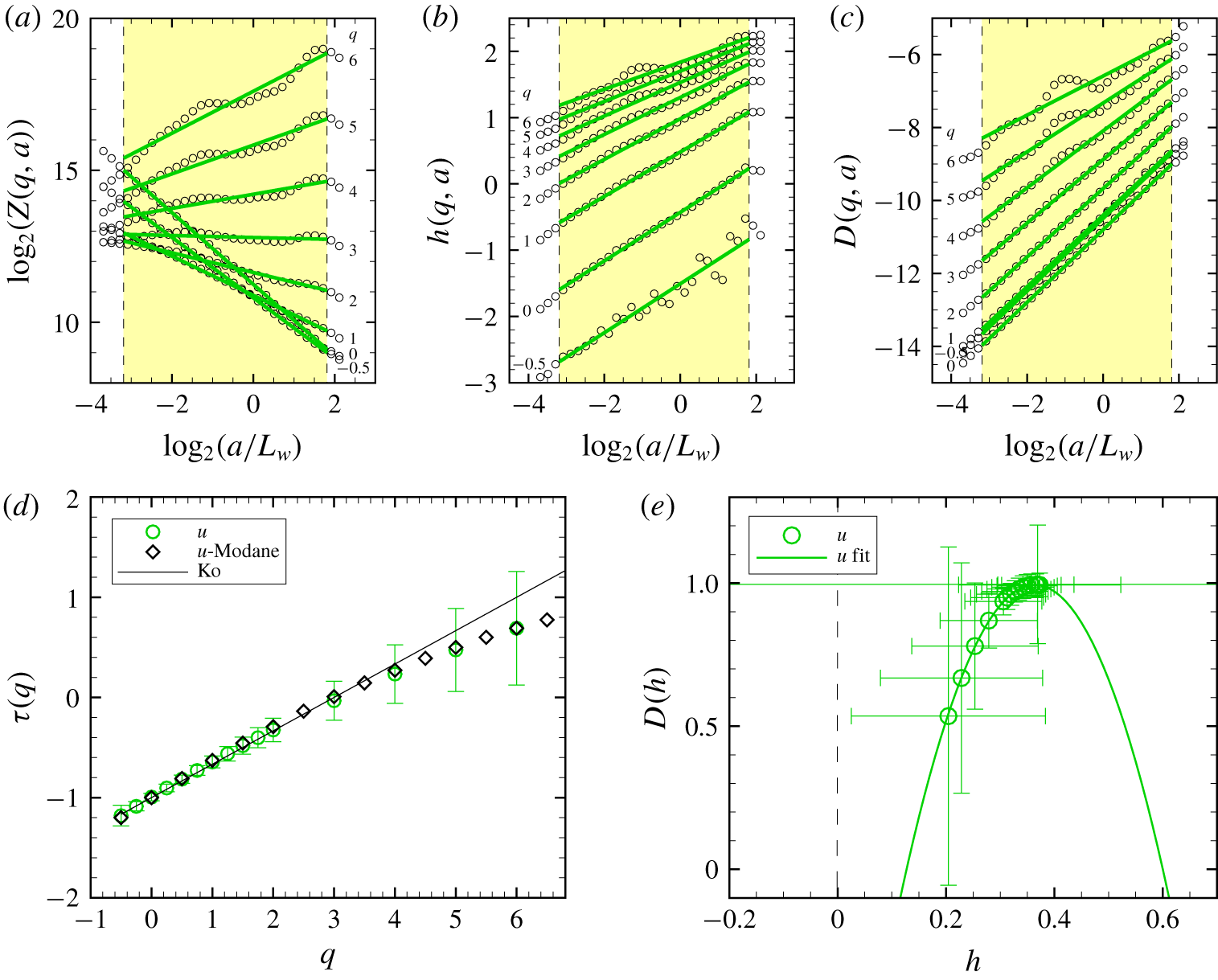
Unlike  $\unicode[STIX]{x1D703}$, the WTMM analysis of
 $u$ for run 7 reveals only one scaling regime covering the two scaling regimes I and II of
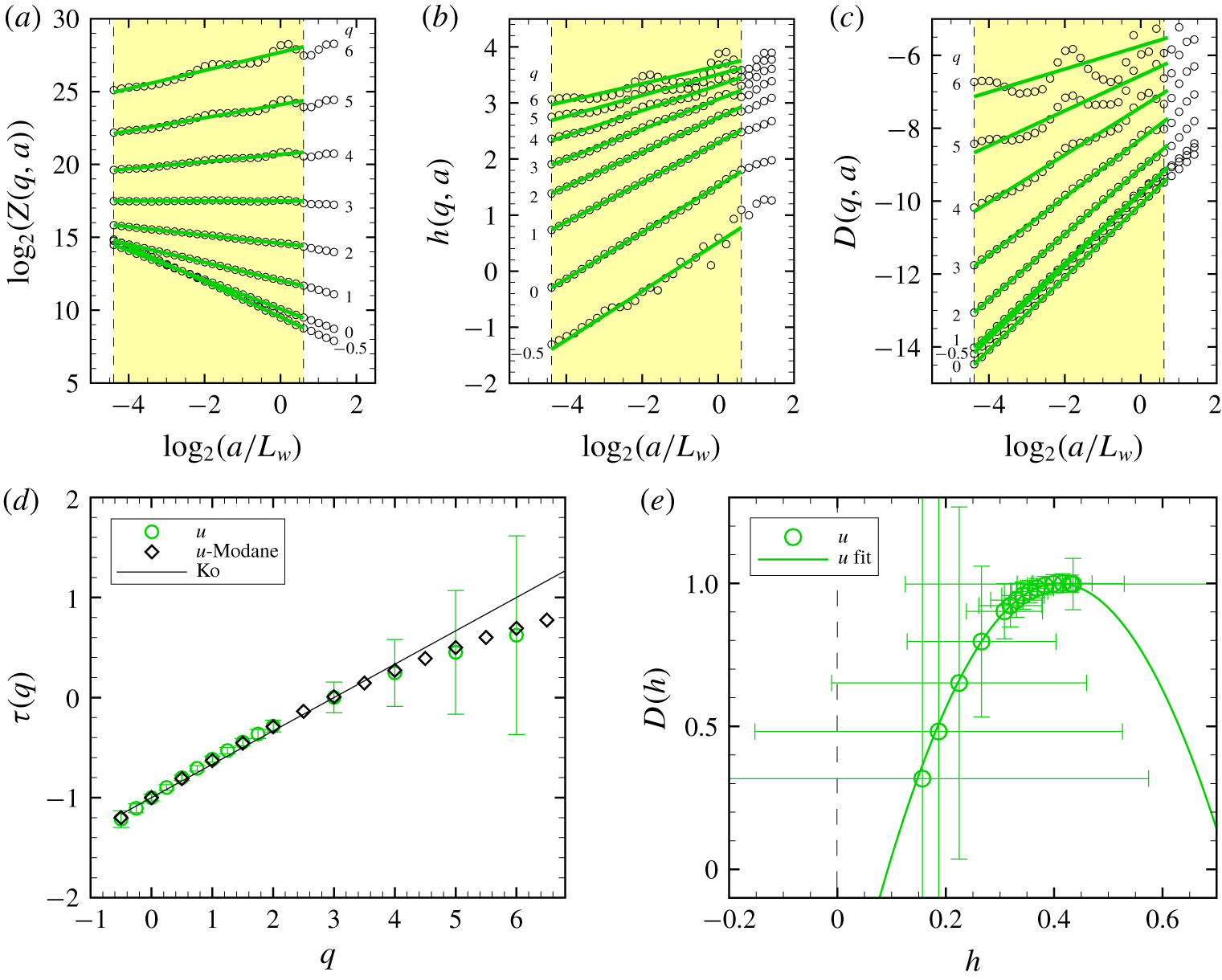
 $\unicode[STIX]{x1D703}$ (figure 6). The
 $\unicode[STIX]{x1D70F}(q)$ spectrum of
 $u$ fits well with that observed for
 $u$ in the Modane wind-tunnel experiment, with no sign of saturation. Importantly, as in Modane and in Antonia et al. (Reference Antonia, Hopfinger, Gagne and Anselmet1984),
 $u$ fluctuations exhibit a lower intermittency coefficient (
 $c_{2}^{u}=0.04\,\pm <0.01$ on average) than
 $\unicode[STIX]{x1D703}$ fluctuations (
 $c_{2}^{\unicode[STIX]{x1D703}}=0.09\pm 0.01$ on average) (table 2).
Multifractal analysis of the canopy-top longitudinal velocity under an unstable atmospheric regime (run 7 in table 1) using the WTMM method. (a) Partition function  $\log _{2}(Z(q,a))$ versus
 $\log _{2}(a/L_{w})$. (b)
 $\log _{2}(h(q,a))$ versus
 $\log _{2}(a/L_{w})$. (c)
 $\log _{2}(D(q,a))$ versus
 $\log _{2}(a/L_{w})$. (d) The scaling function
 $\unicode[STIX]{x1D70F}(q)$ versus the moment order
 $q$ estimated by linear regression fit of
 $\log _{2}(Z(q,a))$ versus
 $\log _{2}(a)$, and compared with
 $\unicode[STIX]{x1D70F}(q)$ for the isotropic–homogeneous turbulent flows of Modane and prediction from Kolmogorov (Ko) turbulence theory. (e) The singularity spectrum
 $D(h)$ versus the singularity strength
 $h$ obtained from linear regression fits of
 $\log _{2}(h(q,a))$ and
 $\log _{2}(D(q,a))$ versus
 $\log _{2}(a)$. In (a–c), the yellow box delimits the scaling regimes. The green solid lines represent the linear fit for the scaling regime.
These behaviours of the multifractal spectra of  $\unicode[STIX]{x1D703}$ and
 $u$ fluctuations have been systematically observed in all our runs under unstable conditions (
 $\unicode[STIX]{x1D701}\leqslant -0.15$). The same analyses performed only on the half-length of the signals exhibited the same behaviours, showing that the saturation of the
 $\unicode[STIX]{x1D70F}(q)$ spectrum of
 $\unicode[STIX]{x1D703}$ is not an artefact of the finite length of the signals (result not shown). In stable conditions (
 $\unicode[STIX]{x1D701}\geqslant 0.26$), similar behaviours were also observed although the ramp–cliff patterns in the
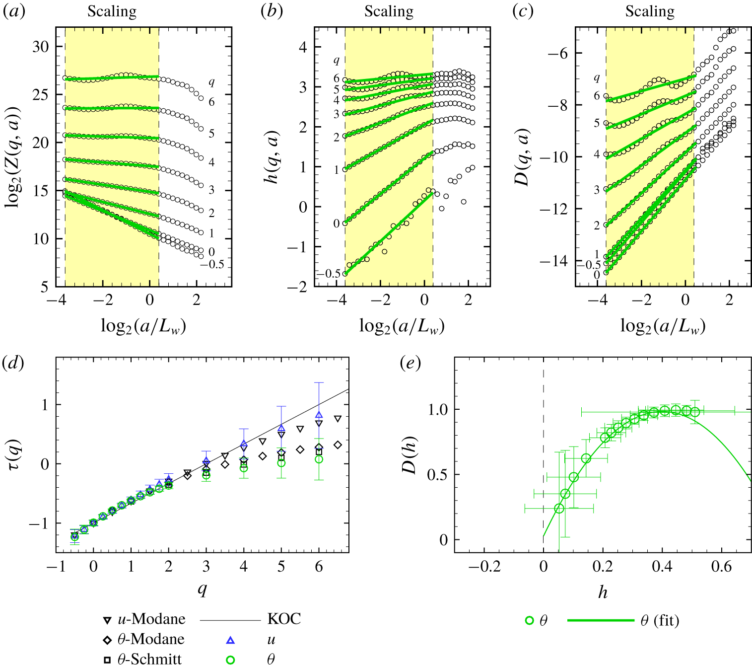
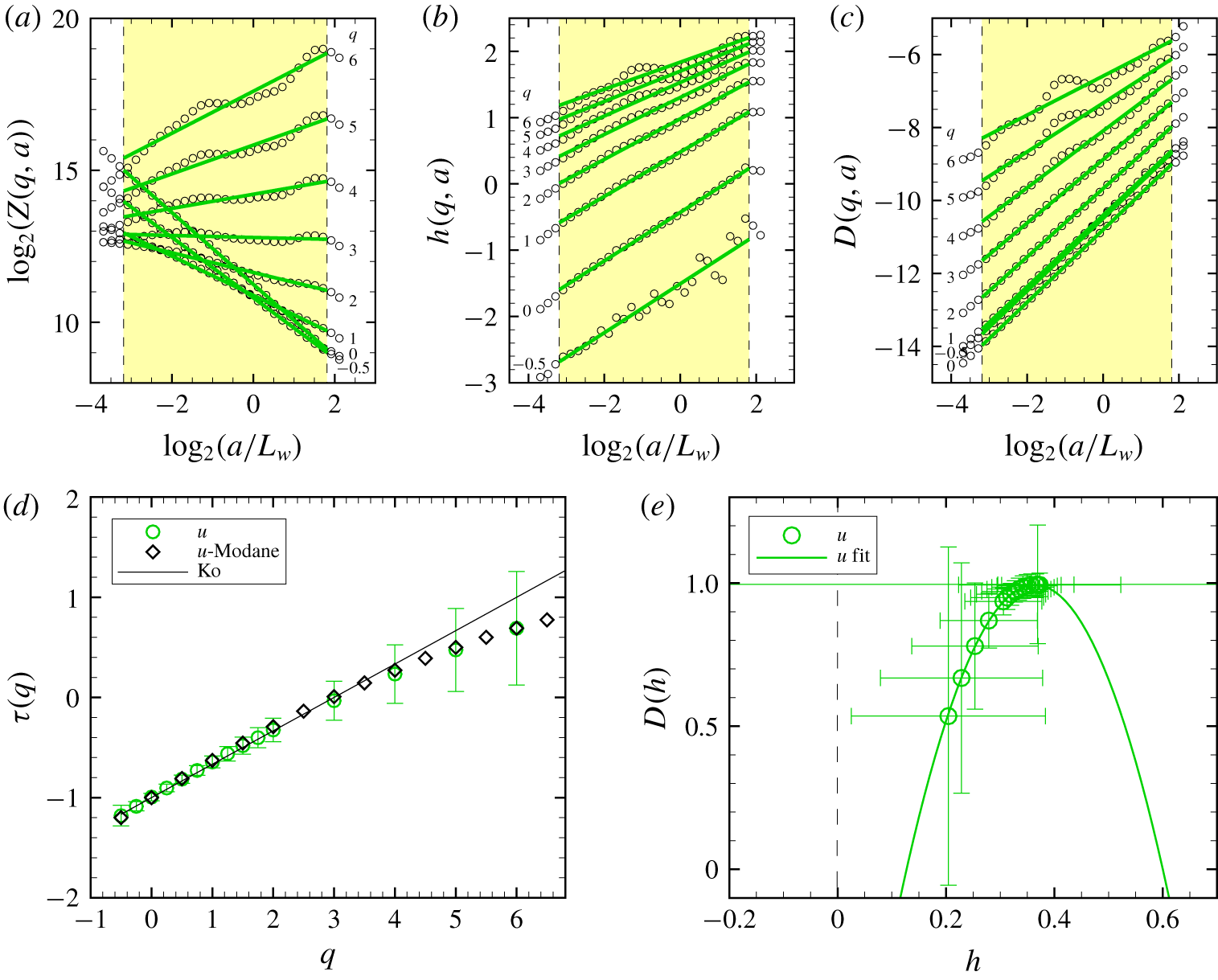
 $\unicode[STIX]{x1D703}$ signal were inverted (see figures 7 and 8 for the run 27). However, in near-neutral conditions, the temperature multifractal spectra exhibit only one scaling regime up to
 $L_{w}$, as for
 $u$, without sign of saturation of
 $\unicode[STIX]{x1D70F}(q)$ (see figure 8 for run 19). The spectra
 $\unicode[STIX]{x1D70F}(q)$ of
 $\unicode[STIX]{x1D703}$ and
 $u$ are both in agreement with those obtained from the Modane wind-tunnel experiment (figure 9d). Importantly,
 $\unicode[STIX]{x1D703}$ fluctuations are still more intermittent than
 $u$ fluctuations (table 2).
Compared to  $\unicode[STIX]{x1D703}$ and
 $u$, the scaling of the partition function of the vertical velocity component
 $w$ was not as well defined at high-order moments. This is probably related to the much smaller integral scale of
 $w$ (table 1). Consequently, the scaling functions
 $\unicode[STIX]{x1D70F}(q)$ and the singularity spectra
 $D(h)$ obtained for
 $w$ are compared with those from
 $\unicode[STIX]{x1D703}$ and
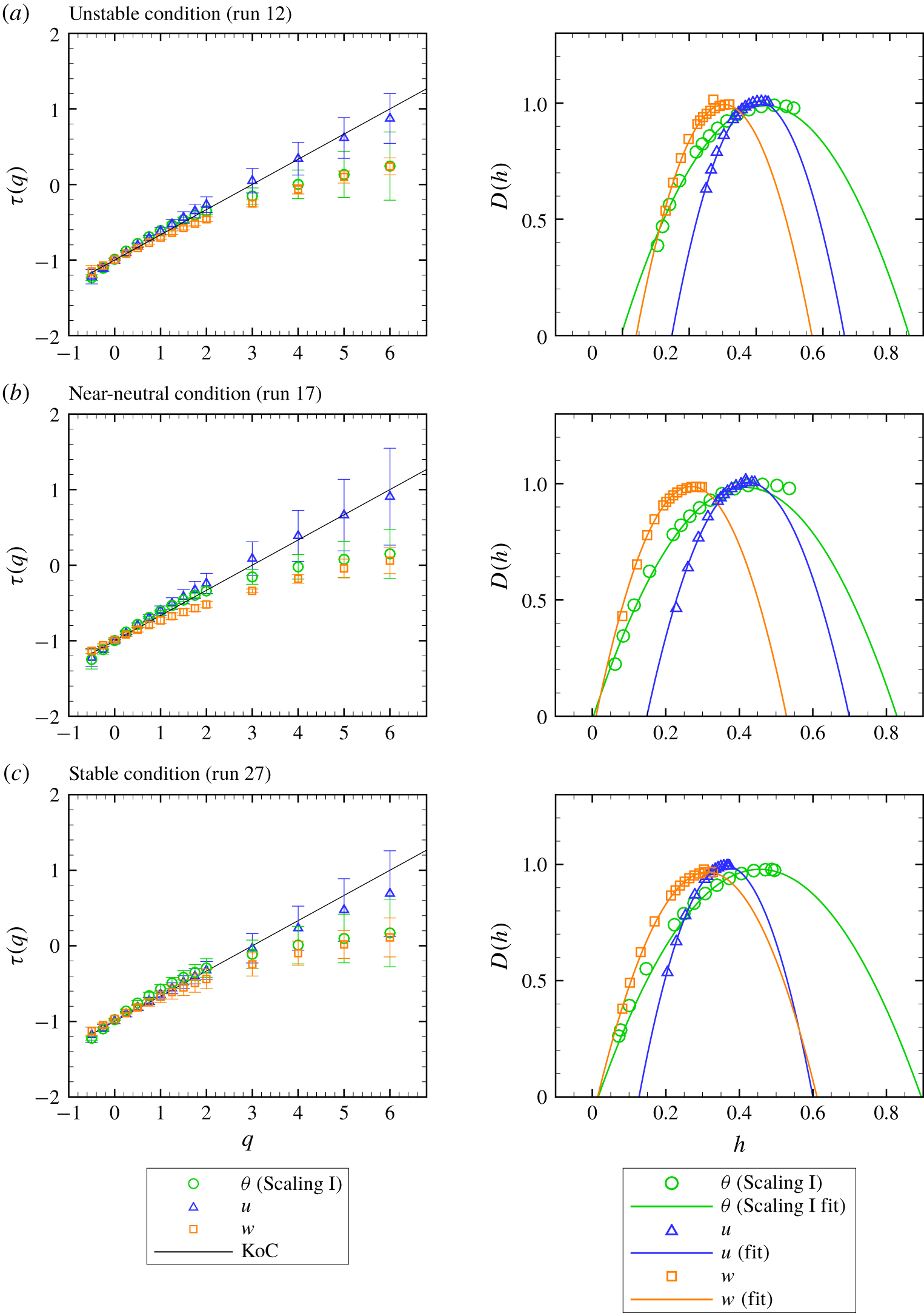
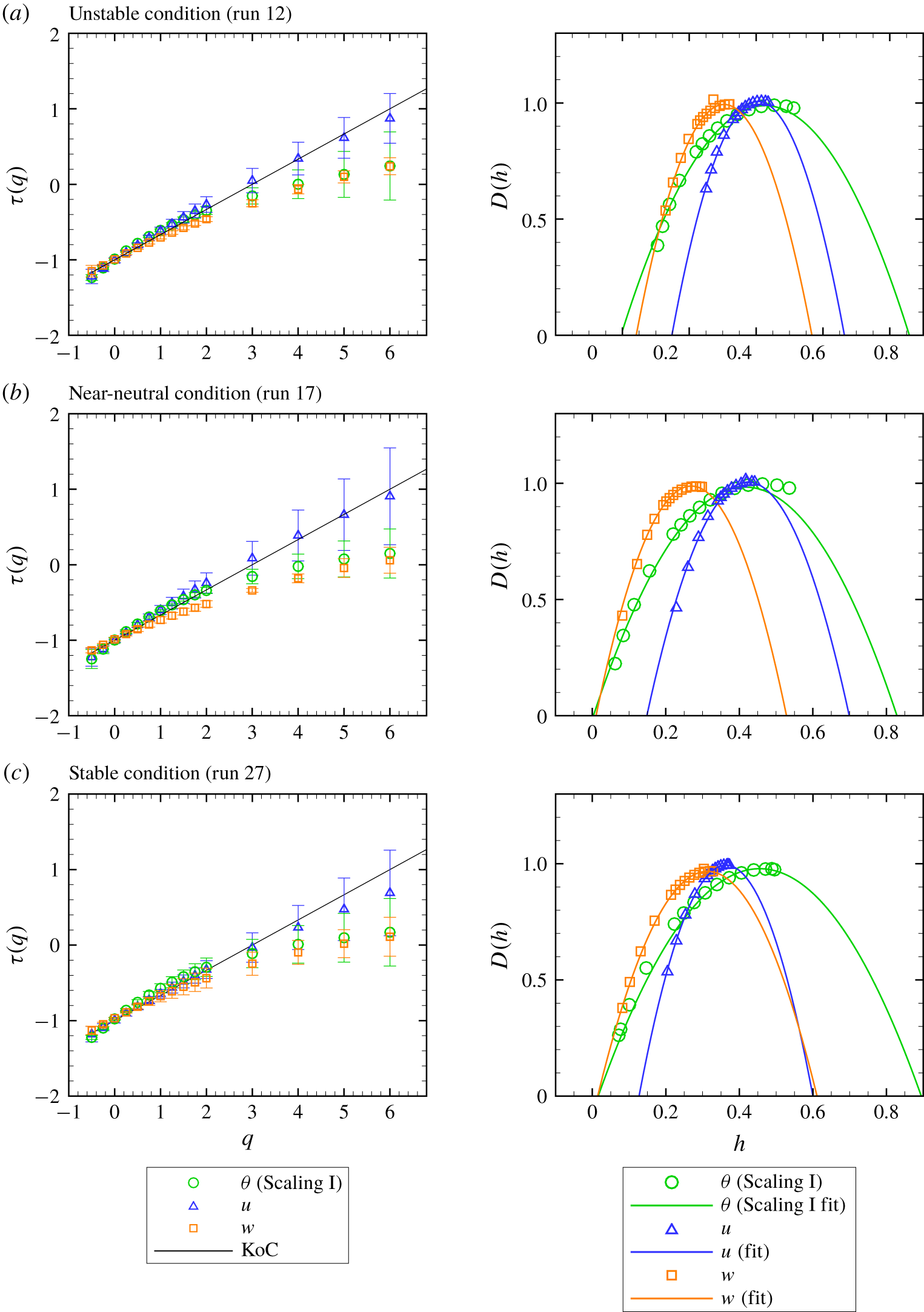
 $u$ for only runs 12 (unstable condition), 17 (near-neutral condition) and 27 (stable condition), at small scales within the inertial convective subrange (figure 10). For larger scales,
 $w$ fluctuations show no scaling regime due to their lower integral scale as compared to those of
 $u$ and
 $\unicode[STIX]{x1D703}$ (table 1). Overall, at fine scales,
 $\unicode[STIX]{x1D70F}(q)$ and
 $D(h)$ exhibit small differences between stability conditions. The scaling exponent
 $\unicode[STIX]{x1D70F}(q)$ of
 $w$ fluctuations appears lower than that of
 $u$ fluctuations, which is consistent with observations from Katul, Porporato & Poggi (Reference Katul, Porporato and Poggi2009), and close to that of
 $\unicode[STIX]{x1D703}$ fluctuations, although the intermittency of
 $w$ (
 $c_{2}$ coefficient) is lower than the one of
 $\unicode[STIX]{x1D703}$ and slightly larger than the one of
 $u$. This is visible from the narrower singularity spectra
 $D(h)$ of
 $w$ as compared to the singularity spectra of
 $\unicode[STIX]{x1D703}$. The mean strength of the singularities of
 $w$ (
 $c_{1}$ coefficient or the maximum of the singularity spectra) is stronger (lower
 $c_{1}$ coefficient) than the mean strength of
 $\unicode[STIX]{x1D703}$ singularities. This means that the fluctuations of
 $w$ are on average sharper than those of
 $\unicode[STIX]{x1D703}$, although the strongest fluctuations reach a similar strength in both signals (
 $h=0$).
Comparison of the scaling functions  $\unicode[STIX]{x1D70F}(q)$ (left panels) and singularity spectra
 $D(h)$ (right panels) obtained for
 $u$,
 $w$ and
 $\unicode[STIX]{x1D703}$ in the first scaling regime, for an unstable (a), near neutral (b) and stable (c) regime.
3.2 Wavelet skewness and flatness factors of $\unicode[STIX]{x1D703}$ and $u$


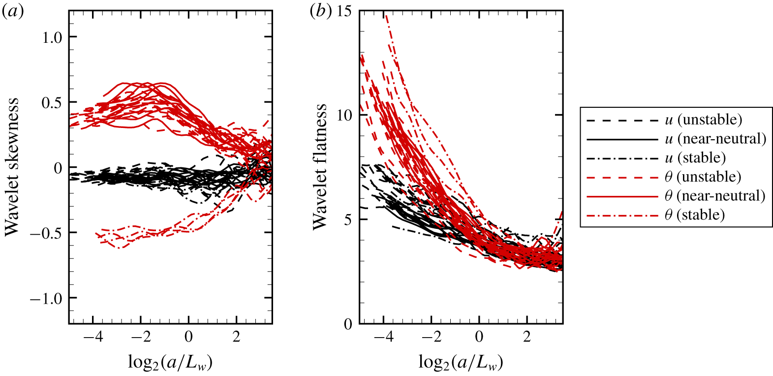
To confirm previous results on the larger intermittency of  $\unicode[STIX]{x1D703}$ fluctuations than
 $u$ fluctuations independently of the thermal stratification, the wavelet skewness factor (SF) and flatness factor (FF), i.e. skewness and flatness of the wavelet coefficients, of
 $u$ and
 $\unicode[STIX]{x1D703}$ are presented in figure 11 for different stability regimes. Both factors were defined as follows:
 $$\begin{eqnarray}\text{SF}_{f}(a)=\langle T_{\unicode[STIX]{x1D713}}[f]{(t,a)^{\prime }}^{3}\rangle /\langle T_{\unicode[STIX]{x1D713}}[f]{(t,a)^{\prime }}^{2}\rangle ^{3/2},\end{eqnarray}$$
and
 $$\begin{eqnarray}\text{FF}_{f}(a)=\langle T_{\unicode[STIX]{x1D713}}[f]{(t,a)^{\prime }}^{4}\rangle /\langle T_{\unicode[STIX]{x1D713}}[f]{(t,a)^{\prime }}^{2}\rangle ^{4/2},\end{eqnarray}$$
where  $f$ is either
 $u$ or
 $\unicode[STIX]{x1D703}$, the brackets refer to time average and
 $T_{\unicode[STIX]{x1D713}}[f](t,a)^{\prime }=T_{\unicode[STIX]{x1D713}}[f](t,a)-\langle T_{\unicode[STIX]{x1D713}}[f](t,a)\rangle$;
 $\langle T_{\unicode[STIX]{x1D713}}[f]{(t,a)^{\prime }}^{2}\rangle$ is the variance of the wavelet transform of
 $f$,
 $\langle T_{\unicode[STIX]{x1D713}}[f]{(t,a)^{\prime }}^{3}\rangle$ its moment of order 3 and
 $\langle T_{\unicode[STIX]{x1D713}}[f]{(t,a)^{\prime }}^{4}\rangle$ is its fourth-order moment.
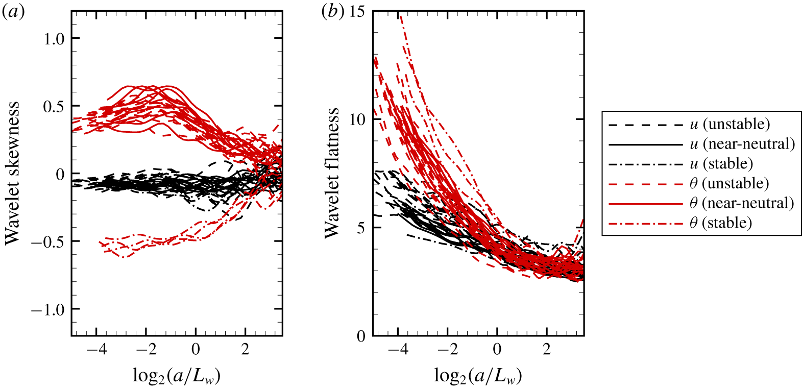
Overall,  $u$ fluctuations appear in near-isotropic state with near-zero SF values, around - 0. 1 to - 0. 2, independently of the stability (figure 11a). This is consistent with the observed similarity at small scales (
 $a<L_{w}$) between the multifractal characteristics of
 $u$ and those observed in homogeneous–isotropic turbulence (Modane, figure 5). The SF values of
 $u$ obtained here for the mixing-layer-type flow prevailing at the canopy top are smaller than the values reported in atmospheric shear flows (Katul & Parlange Reference Katul and Parlange1994; Basu et al. Reference Basu, Foufoula-Georgiou, Lashermes and Arnéodo2007). The SF values of
 $\unicode[STIX]{x1D703}$ are larger in magnitude, with negative values (- 0. 5) in stable conditions and positive values (+ 0. 5) in unstable conditions, reflecting the well-known anisotropic state of scalar turbulence at small scales (Sreenivasan Reference Sreenivasan1991). The sign difference of
 $\text{SF}_{\unicode[STIX]{x1D703}}$ between unstable and stable conditions is consistent with previous observations (Katul & Parlange Reference Katul and Parlange1994, Reference Katul and Parlange1995), and was suspected to be related to the type of turbulence regime: isolated shear-overturning events in the stable condition and updraft–downdraft events in the unstable regime (Mahrt & Gamage Reference Mahrt and Gamage1987).
The flatness factors increase with decreasing scale, starting with Gaussian values (+ 3) near the integral scale (figure 11b). As expected, this increase is stronger for  $\unicode[STIX]{x1D703}$ leading to larger FF values at smaller scales. This is consistent with the larger fine-scale intermittency of
 $\unicode[STIX]{x1D703}$ compared to
 $u$ obtained from our multifractal analysis. This difference between
 $\text{FF}_{\unicode[STIX]{x1D703}}$ and
 $\text{FF}_{u}$ is also in agreement with observations from Katul & Parlange (Reference Katul and Parlange1994, Reference Katul and Parlange1995). Overall, the flatness factors appear weakly dependent on the stability. Only the
 $\unicode[STIX]{x1D703}$ flatness factors seem larger in stable conditions.
The small differences of SF and FF between non-neutral and near-neutral conditions do not permit us to distinguish an effect related to the presence or absence of saturation of the scaling exponent of  $\unicode[STIX]{x1D703}$ observed in the previous section.
4 Discussion
Our multifractal analysis suggested a substantial similarity at small scales ( $a<L_{w}/4$) between the multifractal characteristics of canopy-top
 $u$ and
 $\unicode[STIX]{x1D703}$ fluctuations and those observed in homogenous–isotropic turbulence, for at least moment order
 $q$ of up to 6. This was observed from the agreement of the scaling exponents
 $\unicode[STIX]{x1D70F}(q)$ of
 $u$ and
 $\unicode[STIX]{x1D703}$ in the scaling regime I with the well-known multifractal properties of isotropic–homogeneous turbulence (Arneodo et al. Reference Arneodo, Bacry and Muzy1995; Schmitt Reference Schmitt2005). This similarity is probably explained by the canopy-top mixing-layer-type flow weakening the anisotropy and inhomogeneity of the above atmospheric surface-layer shear flow. In near-neutral conditions, this similarity extends up to
 $L_{w}$. To our knowledge, this represents the first demonstration of the analogy between the fine-scale turbulence at the canopy top and that in an isotropic–homogeneous flow.
Under thermal stratification conditions (unstable or stable), steep cliffs (fronts) of large temperature gradients start to contaminate and saturate the multifractal spectra of  $\unicode[STIX]{x1D703}$ fluctuations from high moment orders
 $q$, while the multifractal spectrum of
 $u$ fluctuations remains similar to that in near-neutral conditions. This saturation due to cliff singularities was demonstrated for run 7 by the equivalence between the value of the scaling exponent at saturation (
 $\unicode[STIX]{x1D70F}_{sat}=-0.37$ in figure 5d) and the value of the singularity spectrum for cliff singularities
 $D_{II}(h=0)=0.37$. This is further illustrated in figures 2(c) and 3(c) where cliffs dominate the WTMM lines for the scale range of the scaling regime II, while at smaller scales (regime I), the cliff singularities become embedded by numerous singularities of lower intensities. This saturation of the
 $\unicode[STIX]{x1D703}$ scaling exponent due to cliff structures was observed in all non-neutral runs and is consistent with previous modelling and laboratory measurements of scalar multifractal spectra (Celani et al. Reference Celani, Lanotte, Mazzino and Vergassola2000; Moisy et al. Reference Moisy, Willaime, Andersen and Tabeling2001; Iyer et al. Reference Iyer, Schumacher, Sreenivasan and Yeung2018).
Wavelet skewness (a) and flatness (b) factors of  $u$ and
 $\unicode[STIX]{x1D703}$, as a function of
 $\log _{2}(a/L_{w})$ for the 27 runs, with distinction between unstable, near-neutral and stable conditions.
We argue that this saturation of  $\unicode[STIX]{x1D70F}(q)$ in scaling regime II may reflect an ordered–disordered phase transition in signal singularities with decreasing moment order
 $q$. At high moment orders, strong cliff singularities dominate (ordered phase,
 $h=0$) while at low moment orders, a large range of singularity strengths coexists (disordered phase, large range of
 $h$ values). Such analogy between multifractal formalism and statistical thermodynamics has been demonstrated previously (Jensen, Kadanoff & Procaccia Reference Jensen, Kadanoff and Procaccia1987; Katzen & Procaccia Reference Katzen and Procaccia1987; Arneodo et al. Reference Arneodo, Bacry and Muzy1995), where
 $q$ and
 $\unicode[STIX]{x1D70F}(q)$ play the same role as the inverse temperature and the free energy. In particular, the non-analyticity of
 $\unicode[STIX]{x1D70F}(q)$ has been interpreted as a phase transition occurring at a critical moment order
 $q_{crit}$ (e.g. Barkley & Cumming Reference Barkley and Cumming1990; Schertzer & Lovejoy Reference Schertzer and Lovejoy1992). Hence, this multifractal phase transition is analogous to a phase transition in condensed-matter physics, where systems show regular orientation of atoms with long-range correlation under the low-temperature phase and a random orientation of atoms with no long-range correlation under the high-temperature phase.
To verify this analogy between the saturation of  $\unicode[STIX]{x1D70F}(q)$ and a phase transition, we use the same approach as Arneodo et al. (Reference Arneodo, Bacry and Muzy1995). We assume that
 $\unicode[STIX]{x1D703}$ in scaling regime II is the superposition of two signals, one with the multifractal characteristics of the scaling regime I and the other one corresponding to large-scale ramp–cliff patterns. The partition function of this signal can be then split into two parts:
 $Z_{II}(q,a)=Z_{I}(q,a)+Z_{cliff}(q,a)\sim a^{\unicode[STIX]{x1D70F}_{I}(q)}+a^{\unicode[STIX]{x1D70F}_{sat}}$, where
 $Z_{I}$ and
 $Z_{cliff}$ are the sum of partition functions over the maximum lines created by the first and second signals, corresponding to the scaling laws
 $a^{\unicode[STIX]{x1D70F}_{I}(q)}$ and
 $a^{\unicode[STIX]{x1D70F}_{sat}}$, respectively, in the limit
 $a\rightarrow 0^{+}$. In such conditions, a
 $q$ critical value should exist such that
 $$\begin{eqnarray}\unicode[STIX]{x1D70F}_{II}(q)=\left\{\begin{array}{@{}ll@{}}\unicode[STIX]{x1D70F}_{I}(q), & q<q_{crit}\\ \unicode[STIX]{x1D70F}_{sat}, & q\geqslant q_{crit}.\end{array}\right.\end{eqnarray}$$
At the critical point,  $\unicode[STIX]{x1D70F}_{sat}=\unicode[STIX]{x1D70F}_{I}(q_{crit})\approx -c_{0}^{\unicode[STIX]{x1D703}}+c_{1}^{\unicode[STIX]{x1D703}}q_{crit}-c_{2}^{\unicode[STIX]{x1D703}}q_{crit}^{2}/2!$, which leads to
 $$\begin{eqnarray}q_{crit}=\frac{c_{1}^{\unicode[STIX]{x1D703}}}{c_{2}^{\unicode[STIX]{x1D703}}}-\sqrt{\left(\frac{c_{1}^{\unicode[STIX]{x1D703}}}{c_{2}^{\unicode[STIX]{x1D703}}}\right)^{2}+\frac{2}{c_{2}^{\unicode[STIX]{x1D703}}}(-\unicode[STIX]{x1D70F}_{sat}-c_{0}^{\unicode[STIX]{x1D703}})}.\end{eqnarray}$$
For the temperature time series of figure 5, we obtained  $q_{crit}=1.7$. The saturation of
 $\unicode[STIX]{x1D70F}_{II}(q)$ near
 $-0.37$ for
 $q\geqslant q_{crit}$ is in excellent agreement with the
 $D_{II}(h)$ fall off towards + 0. 37 for
 $h=0$ (
 $D_{II}(h=0)=-\unicode[STIX]{x1D70F}_{sat}$). Furthermore, the linear extension of this fall off is tangent to the
 $D_{I}(h)$ spectrum with a slope equal to
 $q_{crit}$ (figure 5e). This last feature is the signature of a phase transition phenomenon. The change of slope of
 $\unicode[STIX]{x1D70F}_{II}(q)$ around
 $q_{crit}$ suggests a first-order phase transition, but this cannot be concluded with certainty. Indeed, the
 $D_{II}(h)$ fall off is not perfectly linear for
 $q$ values surrounding
 $q_{crit}$, and the non-analyticity of
 $\unicode[STIX]{x1D70F}_{II}(q)$ is not perfect around
 $q_{crit}$. This is due to the shifting of the cross-over with
 $q$ between regime I and the saturation regime, weakening the scaling regime II in this transition region (see
 $h(q,a)$ for
 $q$ around 2 and 3 in figure 5b).
For unstable and stable conditions,  $q_{crit}$ ranges between 1.4 and 3.7 and the fractal dimension of the stronger cliffs (
 $h=0$) varies from
 $D(h=0)=0.0$ to 0.40. Both
 $q_{crit}$ and
 $D(h=0)$ do not show a clear trend according to the stability intensity
 $\unicode[STIX]{x1D701}$ (see table 1), which could be due to the varying large-scale meteorological conditions, even for similar stability levels. However, all runs in these stability conditions exhibited a saturation of
 $\unicode[STIX]{x1D70F}(q)$ and the conditions of a phase transition, which demonstrates the robustness of our results.
One striking result from our multifractal analysis is the absence of saturation in the temperature multifractal spectra under near-neutral conditions. This was observed for the 9 near-neutral runs (table 1). This suggests a negligible impact of cliff singularities ( $h=0$) on the statistics of the
 $\unicode[STIX]{x1D703}$ signal. However,
 $\unicode[STIX]{x1D703}$ fluctuations still appear more intermittent than
 $u$ fluctuations (see the
 $c_{2}^{\unicode[STIX]{x1D703}}$ and
 $c_{2}^{u}$ coefficients in table 2), with the same level of intermittency in both unstable and stable conditions. This larger intermittency of
 $\unicode[STIX]{x1D703}$ fluctuations compared to
 $u$ ones, independently of the stability conditions, was further confirmed by the larger increase of the
 $\unicode[STIX]{x1D703}$ wavelet flatness factor than the
 $u$ one with decreasing scale (figure 11). This result is a strong indication that the statistical contribution of the ‘cliffs’ is not important enough (
 $D(h=0)=0$) to account for the stronger intermittency of
 $\unicode[STIX]{x1D703}$ fluctuations when compared to corresponding
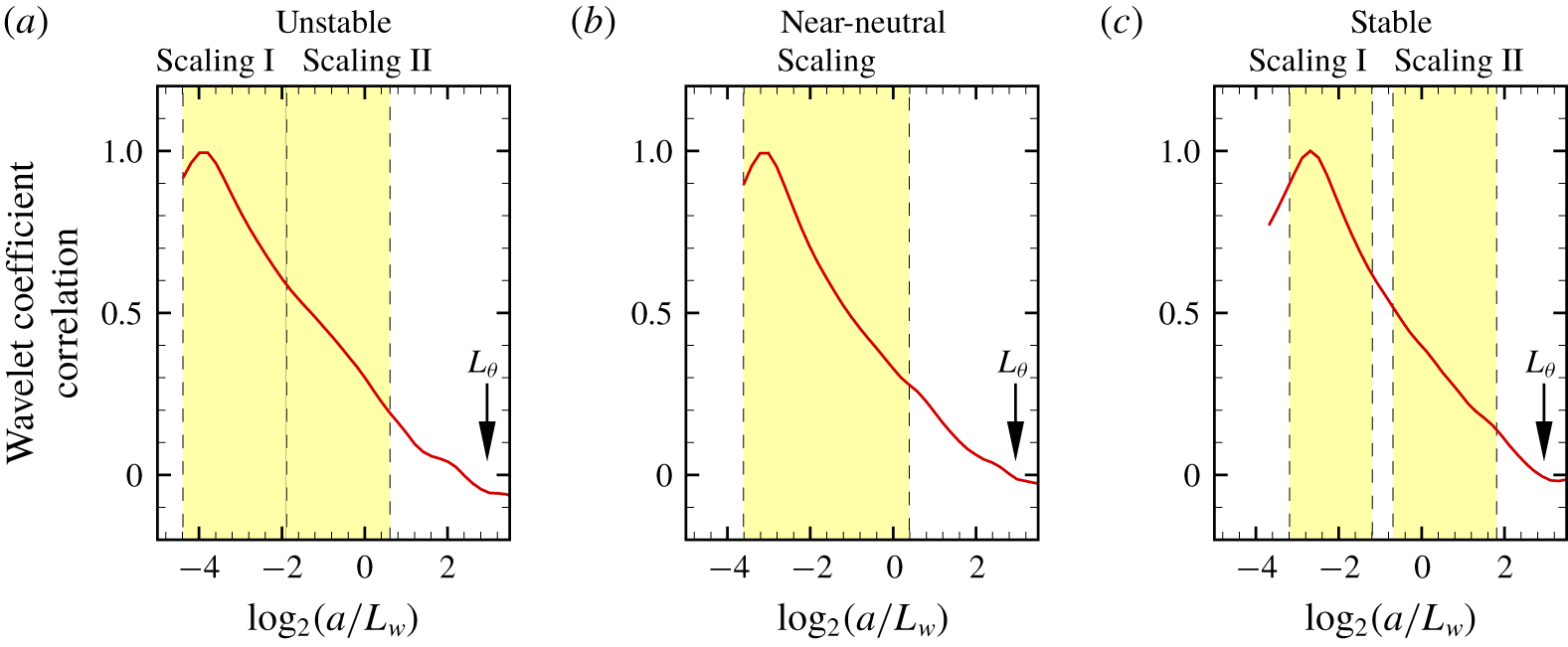
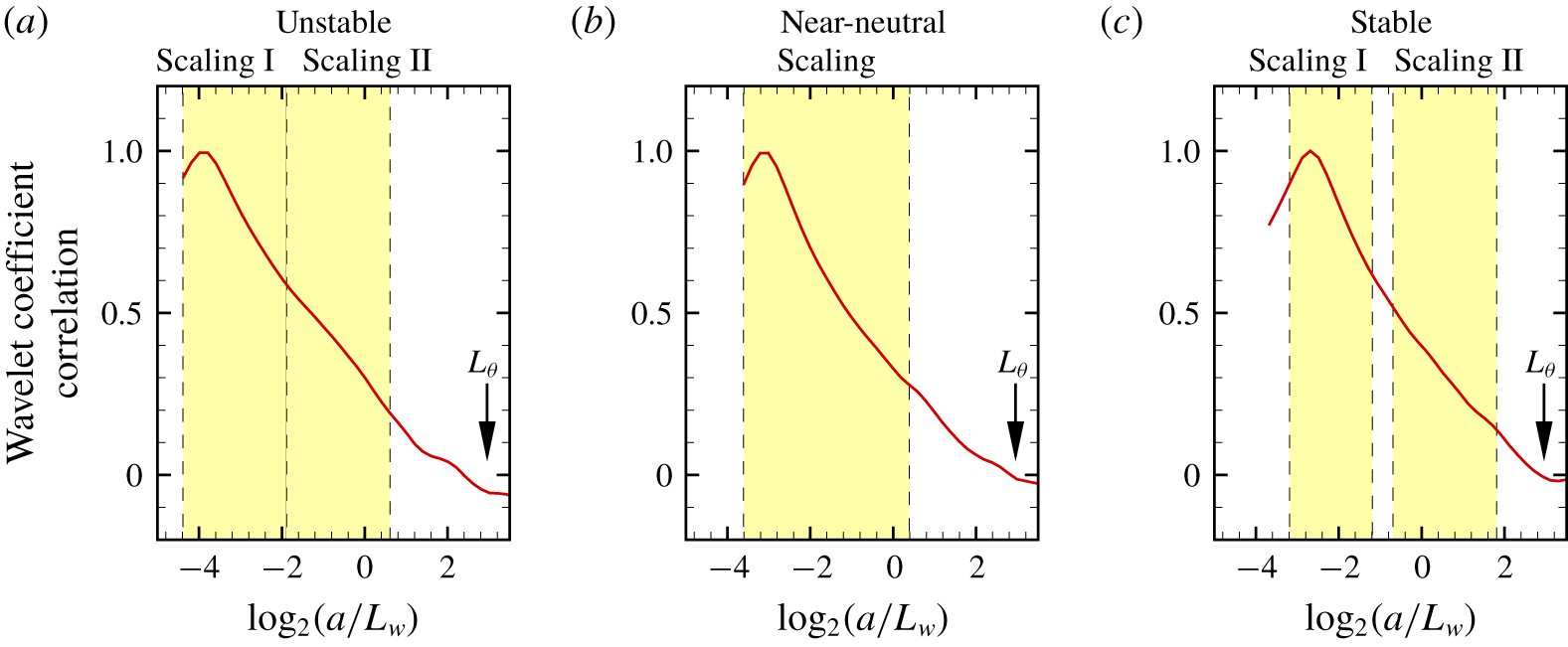
 $u$ fluctuations. This is also confirmed by the poor correlation of the fine-scale
 $\unicode[STIX]{x1D703}$ wavelet coefficients with the near-integral-scale ones, as illustrated in figure 12 for runs 7, 19 and 27 (unstable, near-neutral and stable cases). We suspect that the progressively invaded influence of the strongest singularities (cliffs) with increasing moment order
 $q$, from large to small scales, might lead to the saturation as well of the scalar scaling exponent at small scales (scaling regime I) for
 $q$ values larger than the maximum
 $q$ value considered in this study (
 $q=6$), however, these rare and extreme singularities should be statistically insignificant and could not explain the larger intermittency of scalar fluctuations.
Correlation between the fine-scale modulus of the temperature wavelet transform (within the first scaling regime) and the equivalent larger-scale modulus for an unstable (run 7), near-neutral (run 19) and stable (run 27) regimes. The yellow boxes delimit the scaling regimes. The black arrows indicate the position of the integral scale. This figure confirms for all stability conditions the negligible correlation between  $|T_{\unicode[STIX]{x1D713}}[\unicode[STIX]{x1D703}]|$ within the scaling regime I and
 $|T_{\unicode[STIX]{x1D713}}[\unicode[STIX]{x1D703}]|$ near the integral scale of
 $\unicode[STIX]{x1D703}$ fluctuations (
 $L_{\unicode[STIX]{x1D703}}$). This means that fine-scale
 $\unicode[STIX]{x1D703}$ fluctuations are weakly impacted by large-scale ramp–cliff structures.
This statistically limited contribution of cliff structures to the intermittency of scalar fluctuations contrasts with the Zorzetto et al. (Reference Zorzetto, Bragg and Katul2018) findings on the persistence of the signature of integral-scale ramp–cliff structures on  $\unicode[STIX]{x1D703}$ fluctuations, well within the inertial convective subrange, explaining the larger intermittency of
 $\unicode[STIX]{x1D703}$ fluctuations. We suspect that the mixing-layer-type flow prevailing at the top of our canopy dampens the memory of the integral-scale eddy structures as opposed to shear-layer flow located far above surface roughness elements of Zorzetto et al. (Reference Zorzetto, Bragg and Katul2018).
Our findings suggest that the scalar intermittency at fine scales has more of an internal origin, built from the fluctuation dissipation rate, than an external one, coming from large-scale external forcing (cliffs). Interestingly, the values of the intermittency coefficients  $c_{2}^{\unicode[STIX]{x1D703}}$ (0. 09 ± 0. 01 on average) are close to those observed for Lagrangian velocity fluctuations in turbulent flows (0. 08 ± 0. 01 (Chevillard et al. Reference Chevillard, Roux, Leveque, Mordant, Pinton and Arneodo2003)). Hence, the dynamic of scalar fluctuations appear closer to the dynamic of Lagrangian velocity fluctuations than to that of Eulerian velocity fluctuations. This might be considered for explaining the larger intermittency of scalar fluctuations.
5 Summary
Under unstable and stable conditions, i.e. daily warming and nocturnal cooling conditions, our analysis revealed a saturation of the scaling exponent of the canopy-top air temperature ( $\unicode[STIX]{x1D703}$) fluctuations above a critical moment order, unlike that of the longitudinal wind velocity (
 $u$) fluctuations. This saturation is related to the sharp temperature fronts bordering the ramp–cliff patterns present in the
 $\unicode[STIX]{x1D703}$ signal. This suggests an ordered–disordered phase transition occurring at this critical moment order. Under near-neutral conditions, no such phase transition was observed while
 $\unicode[STIX]{x1D703}$ fluctuations are still more intermittent at fine scales than
 $u$ fluctuations. Hence, conversely to previous studies that suggested large-scale ramp–cliff structures as responsible for the larger intermittency of scalar turbulence at fine scales than that of velocity fluctuations, our multifractal analysis applied to canopy-top mixing-layer-type flow shows that the statistical contribution of the ‘cliffs’ is not significant enough to explain the stronger intermittency of
 $\unicode[STIX]{x1D703}$ fluctuations. Our findings open a new avenue on scalar turbulence intermittency, with an analogy to a phase transition of the invaded influence of the strongest singularities (cliffs) with increasing moment order, from large to small scales.
Acknowledgements
We would like to thank (i) E. Lamaud, J.-M. Bonnefond and D. Garrigou for their contribution to the field data collection, and (ii) C. Chipeaux and D. Loustau for their help with our experiment set-up at the Salles ICOS station. Financial support from the Department ‘Environnement et Agronomie’ of INRA is gratefully acknowledged. Finally, we thank the three anonymous reviewers for their helpful comments.
Declaration of interests
The authors report no conflict of interest.