1. Introduction and summary

An old question in economics is this: is it right to think of the stance and effects of monetary policy in terms of interest rates and asset prices—or are these things better measured by the size and growth of banks’ balance sheets, whether that of the central bank (‘narrow money’) or commercial banks (‘broad money’Footnote ¹)?

Old it may be, but this question throws up a couple of others that are relevant today.

First, is the inflation we are experiencing mainly the result of the growth in broad money in 2020—and were both the ‘inevitable’ result of the QE conducted that year, as some have said?

Second, how does the MPC take account of asset sales (‘QT’) in its economic forecasts—does that not require an additional and explicit estimate of its impact on activity and inflation?

Given the extraordinarily high inflation, we have been experiencing in the past couple of years, and the use of ‘unconventional’ policy over the past decade or so, these are important and legitimate questions. That is my excuse, at least, for the inordinate length of this speech (for which I apologise). I have attempted to summarise the main points in this introduction.

In some ways, the opening question—should we think of the effects of monetary disturbances in terms of prices (interest rates and asset prices) or quantities (monetary aggregates)—draws the contrast between the two a little too starkly. They are not mutually exclusive. In the so-called ‘IS-LM’ model, through which many people are introduced to macro-economics, a rise in the supply of money does eventually lead to a proportionate rise in consumer prices. It is just that it operates via interest rates. That is because, as long as people are free to borrow and lend, demand in these models is fully pinned down by current and (expected) future real interest rates. The expansionary effect of an injection of money therefore relies on its first depressing the yield curve, and the stance of policy is fully captured by the prevailing level of interest rates (relative to some underlying, ‘neutral’ level).

If this core theory appears to favour prices over quantities, then the data too would seem to lean in that direction—or, at least, to caution against too crude an interpretation of the monetary aggregates. History demonstrates that shifts in the quantity of money have often been driven—or at least accompanied—by shifts in the demand for deposits (i.e. what the private sector would like to hold for a given level of spending). Following the financial liberalisation earlier that decade, banks began during the 1980s to pay interest on standard deposit accounts. This increased their attractiveness, relative to other ‘stores of wealth’—they were not the precursor to higher spending and inflation—and broad money growth remained stubbornly high even as inflation declined sharply (at least until the boom at the end of the decade). For similar reasons, it also grew rapidly throughout the first 15 years of inflation targeting (1992–2007).

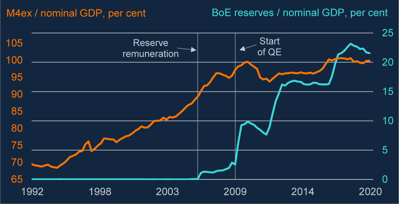
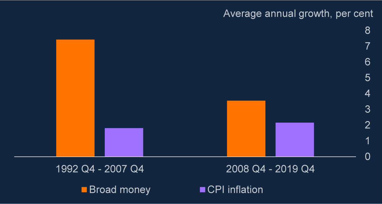
Nor is there a tight correspondence between ‘narrow’ and ‘broad’ money. QE involves the creation of central bank reserves to buy financial assets (usually government debt). So, in the decade or so that passed between the first use of the policy in 2009 and the onset of the pandemic, reserves rose very significantly. Yet broad money growth was significantly slower than it had been before the crisis (chart 1). And, in both periods, average inflation was close to 2 per cent (chart 2).

Chart 1.

Reserve creation neither necessary nor sufficient for strong growth of broad money

Note: Unless stated otherwise ‘broad money’ refers to M4 excluding intermediate other financial corporations (M4ex). This is available from 1997 and projected backwards using aggregate M4 growth before then.

Source: ONS, Bank of England and Bank calculations.

Chart 2.

Broad money growth slowed significantly after the financial crisis, inflation still close to 2 per cent

Source: ONS, Bank of England and Bank calculations.

None of this means that at the margin (holding everything else fixed) QE does not add to broad money or ultimately to the level of prices. Nor does it imply that the quantity measures are never useful or important. It would be as wrong categorically to ignore monetary aggregates as it would to assume that they are the only thing you need to consider.

As far as the theory is concerned, people cannot always borrow and lend freely. In the presence of these and other ‘financial frictions’, the availability of liquid assets can matter for spending, independently of interest rates. Besides, interest rates themselves matter only relative to some ‘neutral’ rate that cannot be observed directly. So, in practice, monetary policymakers should always pay attention to other—indeed any—indicators of incipient inflationary pressure. And although changes in banks’ deposits have often been driven by shifts in demand, there are times when they look more supply-led.

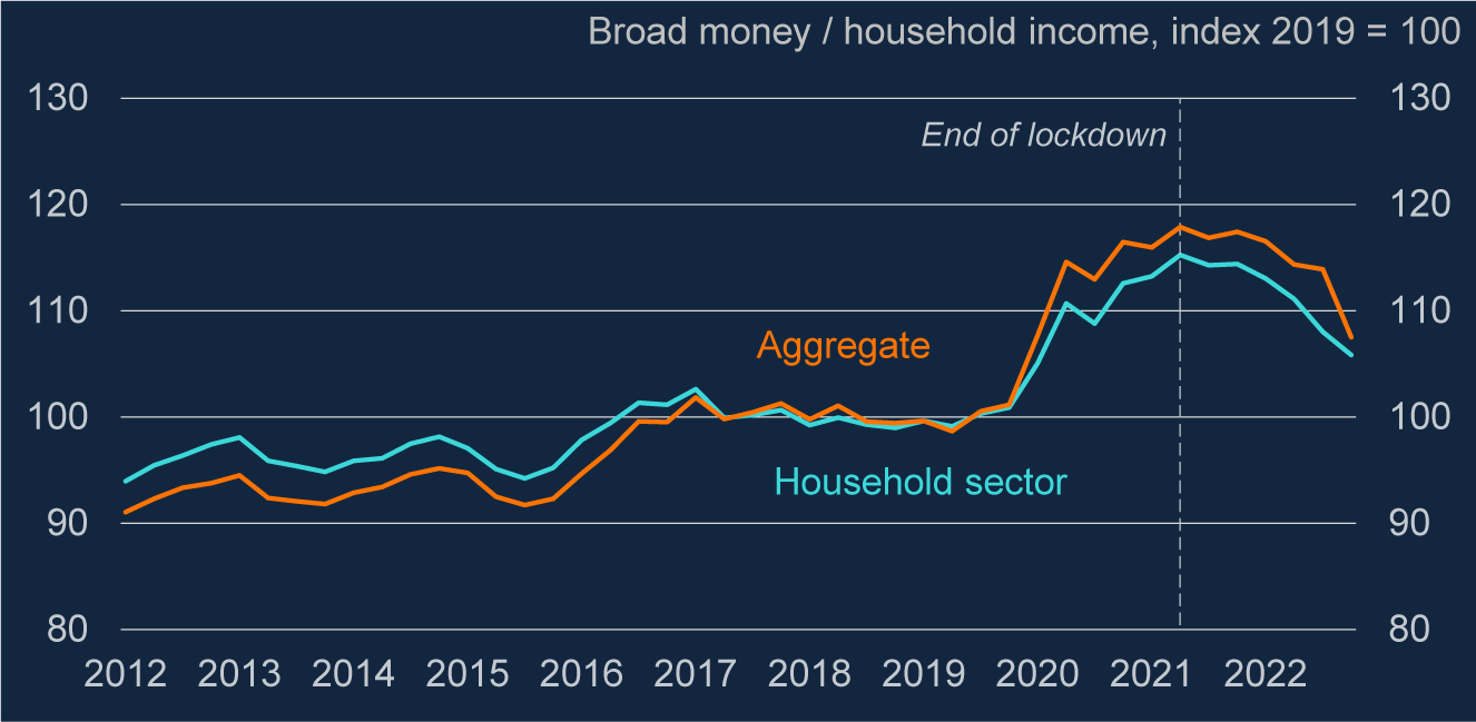
Arguably, the surge in broad money in 2020 looks like one such episode. Supported by the furlough scheme, and because their spending was held back by the lockdowns, households accumulated significant deposits during the pandemic (chart 3). While not literally a ‘helicopter drop’, this came quite close to an exogenous increase in the stock of household (and aggregate) money. Monetary authorities (including the MPC) certainly asked themselves at the time whether, independently of the level of the yield curve, the liquid nature of these assets would give a particular impetus to consumer spending once the lockdowns were lifted.

Chart 3.

Households accumulated significant deposits during the pandemic

Note: Household income is annualised quarterly nominal disposable income. It is defined as the household sector’s gross disposable income adjusted for the change in pension entitlements.

Source: ONS, Bank of England and Bank calculations.

However, what history does demonstrate is that movements in broad money can (and usually do) occur independently of developments in the size of the central bank’s balance sheet. Commercial banks can create and withdraw deposits without any commensurate change in their reserve holdings at the central bank. If the jump in broad money during the pandemic really was the ‘inevitable’ consequence of the QE at the time, one presumably would expect to have seen the same after every preceding set of asset purchases. As chart 2 illustrates, that is not the case.

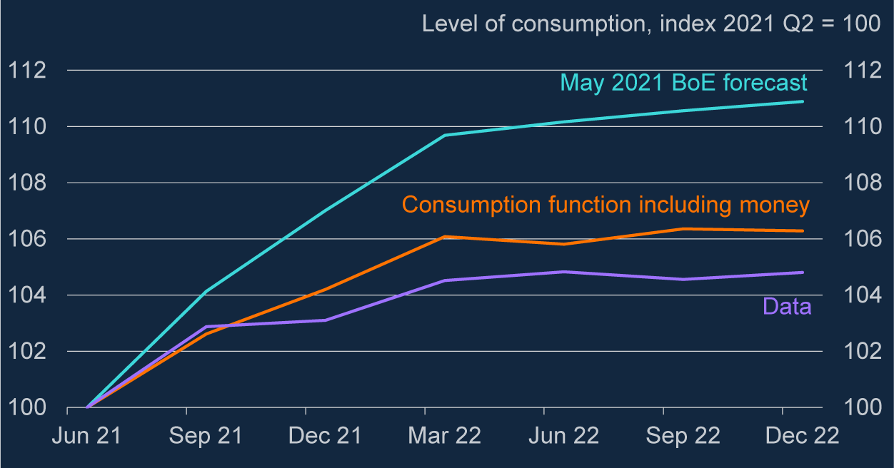
And even if it looks more ‘supply’ than ‘demand’ led—in the sense that these were ‘excess’ deposits—I think the evidence also makes it hard to argue that they alone can explain the inflation that has followed. For one thing, the growth of consumer spending over the following year, once the pandemic restrictions were lifted, was actually weaker than either the MPC—or, indeed, a simple, money-driven consumption function—had predicted (chart 4).

Chart 4.

MPC over-predicted demand coming out of the pandemic

Note: The money-based forecast is based on an error correction model of consumption estimated over 1992–2019 that includes separate terms for liquid assets and illiquid assets in both the long-term relationship and short-term dynamics. It is based on a consumption function set out in Aron et al. (Reference Aron, Duca, Muellbauer and Murata2012).

Source: ONS, Bank of England and Bank calculations.

Nor does the pattern of price rises, over the past couple of years, fit the story. A pure, money-driven inflation affects all prices equally. What we have actually seen are huge shifts in relative prices—first the jumps in those of non-energy traded goods in 2021 and then, in 2022, the enormous rises in the costs of imported food and energy.

The important point here is that, however you measure it—whether in terms of prices (interest rates) or quantities (monetary aggregates)—monetary policy operates with a lag. During that interval, and at least until policy can react to them, there are lots of things—‘shocks and disturbances’ (as the MPC’s remit puts it) that can affect inflation. In this case, it is clear what those have been: the hits to the supply of non-energy goods during the pandemic, to those of energy and food during the war, and the resulting rise in their global prices. Thanks to the significant hit to real incomes they involved, these shocks have also had sizeable second-round effects on domestic wages and prices. As an explanation for the inflation, we have experienced I think this fits the actual data much better than the single fact of strong household money growth during the pandemic.

It is always possible, at least with the benefit of hindsight, to construct an alternative path for monetary policy over the past that would have kept inflation on target, even in the face of these subsequent shocks. But that is not the same thing as saying that the actual policy was ‘inevitably’ going to result in excessive inflation. Simulations suggest that, had that alternative (much tighter) policy path been followed, and then had Russia failed to invade Ukraine, inflation would now be materially below target.

Anyhow, what follows is a walk—rather a long walk, I am afraid—through these various points. Less ink is spilled on the second question, concerning QT: should the MPC not include in its forecasts some identifiable and separate effects of asset sales on activity and inflation? Having argued that the policy is transmitted to demand and inflation largely via asset prices, my answer to this will be ‘no’. The Committee has said that the size of the asset purchase facility (APF), the vehicle through which QE and QT are conducted, will be reduced gradually and predictably and, to that end, announced last September the exact planned reduction of the APF over the following 12 months. As such, it is reasonable to suppose that the impact of QT, even in prospect, is already captured in the prices of assets on which we condition our forecasts. To add something else would be to double-count the effect.

2. Macro-models and the determination of demand

As an undergraduate, one of the books I had to read was a collection of essays about monetary economics by one of my lecturers, Frank Hahn. It begins with this rather provocative sentence:

As a newcomer to the subject, I found this a bit concerning (not to say alarming). If economics cannot even say why money exists, how can it hope to explain what it does?

Reading on, one’s concern subsided a bit. Hahn was, by training and inclination, a general equilibrium theorist. For him, as he explained in the very next sentence, ‘the best developed model of the economy’ was the highly stylised description developed by the great economic theorists Ken Arrow and Gerard Debreu. For all its sophistication, the Arrow–Debreu model is one in which, by assumption, trade is entirely costless. In this perfect economy, there is a market and a price for the exchange of any two goods or services—including those for future delivery—without the need for a medium of exchange or any sort of costly financial architecture. So, it is not a huge surprise that, having ruled out at the start the conditions that might require it, this model should ‘have no place’ for money.

What Hahn’s bit of rhetoric does suggest is that you need some sort of financial friction—some departure from the platonic realm of Arrow–Debreu—to explain why money might matter. Take, for example, the relationship that determines consumer spending in many models of the macro-economy. Typically, this originates with a question: how would a forward-looking consumer, able to borrow and lend relatively freely, allocate his or her spending over time? After solving that stylised problem, and a bit of manipulation, you end up with something like this:

(1) $$ C=f(r)\left(\hskip0.1em pW+H\right). $$

Here, in what I have described rather grandly as equation (1)), f(.) is some function of current and future (real) interest rates and the term in brackets is total wealth. Wealth has two components: net financial assets W (with an average real price p) and the present value of current and expected future labour income, or ‘human wealth’ H. (In this set-up, greater ‘consumer confidence’ can be thought of as a rise in those future expected incomes, and therefore this H term.) Higher real interest rates depress both p and H because they increase the rate at which future income is discounted.

Because there is only one market here (in borrowing and lending), the demands of this set-up are not quite as onerous as in Hahn’s ‘best developed model of the economy’, with its multiple barter exchanges. Nor do you have to assume that people can borrow and lend at precisely the same rate of interest (it does matter that they can do so at all). And in practice, estimated relationships of this sort have all sorts of dynamics within them—consumer spending will not adjust instantaneously to shifts in the right-hand-side variables—allowing the model to fit the data that much better.

But the core relationship for consumption, in most macro-models, will have something like (1) within it. And the important thing here, for our purposes, is that there is no identifiable and direct role for money. The same is true of the relationships used to model business investment. So at least according to this description, monetary policy affects demand (and thereby inflation) only to the extent it influences ‘r’ or ‘p’.

You might think that there is another, more direct channel, via the wealth term ‘W’. At least as far as their gross financial assets are concerned, quite a bit of households’ (and overall private-sector) wealth is held in the form of deposits in commercial banks. These also account for the vast majority of money in the economy (sometimes called ‘broad money’).

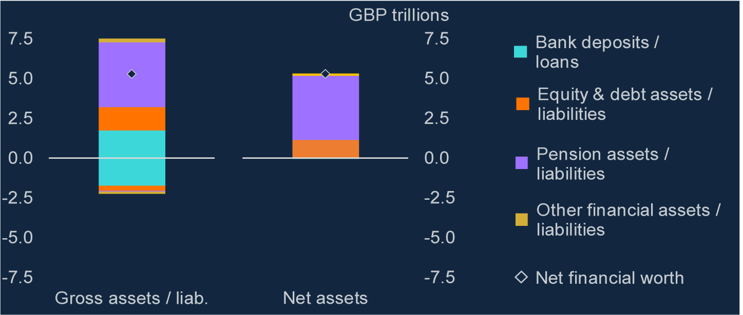
So would not the creation of new deposits add directly to W and boost demand that way, even if there were no change in interest rates or asset prices? The answer is ‘no’. What one has to remember is that, for every pound of deposit liabilities, a bank has on the other side of its balance sheet a pound’s worth of lending, or something like it: a matching obligation from the private sector to the bank. Indeed, it is precisely in the act of extending credit that a commercial bank typically creates ‘new’ (broad) money.Footnote ² So, at least for the private sector as a whole, its interactions with the banking system—deposit claims on the one hand, bank loans on the other—are essentially a wash and do not represent net wealthFootnote ³ (chart 5).

Chart 5.

Households’ deposits matched by what they owe the banks

Note: Financial balance sheet of the household sector, 2022 Q4. Bank deposits are sterling deposits with UK monetary financial institutions (MFIs). Equity and debt assets include other deposits, holdings of debt instruments and equity and investment fund shares/units. Pension assets are insurance and pension schemes. Bank loans include sterling short-term loans from MFIs and loans secured on dwellings. Debt liabilities include other loans to the household sector.

Source: ONS and Bank calculations.

The same is true of new deposits at the central bank (reserves, or ‘narrow money’) created by an open-market purchase of assets (what we now call ‘QE’). QE has sometimes been described as ‘printing money’. I think this is a pretty misleading phrase. It seems to suggest that the central bank simply doles out cash to the private sector, with nothing happening in return. (This kind of ‘helicopter drop’, as the economist Milton Friedman described it, would arguably add to the private sector’s net wealth.Footnote ⁴)

For one thing, however, the money created by QE is not like cash (i.e. the zero-interest instrument described in some textbooks). These days, at least, central bank reserves pay interest.Footnote ⁵ I will come back to this point later on.

Second, central bank money is created only in the process of buying—and therefore removing—an asset from the private sector (usually government bonds). It is not a transfer of wealth—it is an asset swap. As far as the private sector is concerned, QE simply replaces one interest-bearing claim on the public sector (gilts) with another (central bank reserves). Subject to any change in the prices of those assets, there is therefore no difference in the value of the private sector’s overall asset holdings immediately before and after a QE transaction. Just as with commercial bank (‘broad’) money, the creation of new central bank money, by these means at least, does nothing directly to add to the net wealth of the private sector.

And if, therefore, a relationship like (1) prevails, it is only by changing interest rates and asset prices that monetary policy, including so-called ‘unconventional’ policy, can work. These prices are in some sense a ‘sufficient statistic’ for what policy does. Other indicators (including, say, monetary aggregates) would not give you any additional information about its impact.

3. An IS-LM refresher

This dichotomy in the way monetary policy is transmitted is also a feature of the so-called ‘IS-LM’ model of demand.

This is a hardy perennial of macro-economics. Originally written down by John Hicks in 1937, as a distillation of what he viewed to be the essential arguments in Keynes’s General Theory, it still serves as the introduction to the subject for many students.

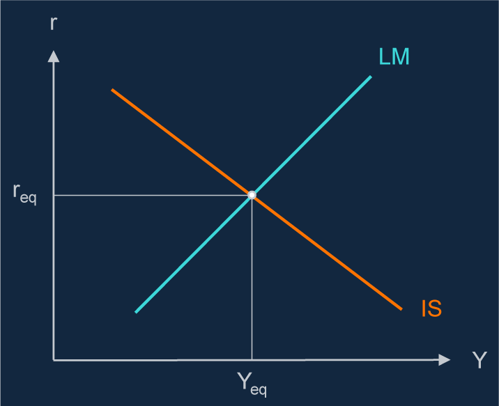
And right at its heart, IS-LM has this same assumption built into it that monetary policy can only affect demand and inflation via interest rates and asset prices (chart 6). As described by the ‘IS’ curve, you need lower yields to boost demand (equation (1) can in fact be seen as a slightly more modern underpinning for this relationship). It is therefore only by those means—only by lowering interest rates and bond yields—that an injection of money, which serves to shift the ‘LM’ curve to the right, can affect spending or ultimately inflation.

Chart 6.

In the IS-LM framework, monetary policy affects demand via prices

Note: ‘Y’ is real output and ‘r’ is the real interest rate. In ‘IS-LM’, ‘IS’ stands for investment-saving and ‘LM’ for liquidity preference-money supply.

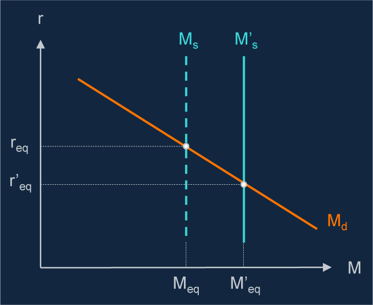
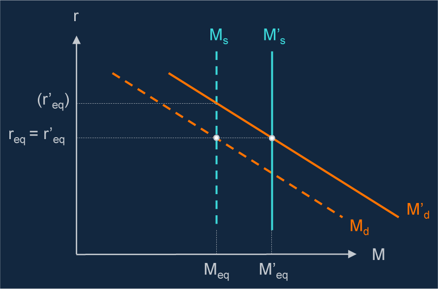
How does that happen? The textbooks—the now-ancient tomes I was given as an undergraduate, at least—describe a process very much like QE. Central banks are said to influence the yield curve by buying and selling government debt in the open market, supplying and withdrawing reserves in the process. In chart 7, the demand for this central bank money is given by the M_D line. It slopes downwards because—all else equal—the willingness of the private sector to hold reserves is meant to decline as the yield on competing assets like bonds goes up. And when the central bank buys bonds, paying for them with newly created reserves (shifting the M_s line to the right), their yields therefore decline. In ‘equilibrium’, for those extra reserves to be willingly held, the competing assets have to become relatively less attractive—hence the decline in yields. Another, perhaps more intuitive, way to think about the effect is that purchasing government bonds directly raises their price (this is the same as a decline in yields). Monetary expansions of this sort therefore raise the supply of central bank reserves, simultaneously lower the level of interest rates and bond yields and, depending on the slope of the ‘IS’ curve, boost demand and subsequently inflation.Footnote ⁶

Chart 7.

Open-market asset purchases by the central bank raise the supply of reserves and push down interest rates

Note: ‘M’ is real money balances and ‘r’ the real interest rate. This model describes the equilibrium in the money market between supply of and demand for money balances, according to Keynes’ theory of liquidity preference. It underpins the LM curve.

The IS-LM model can be a useful way of thinking about monetary policy, and in particular QE.

Chart 7 does have its drawbacks, however, or at least some important oversimplifications. For example, while it may capture some important aspects of how asset purchases work, it is not really an accurate representation of how the conventional policy rate is set. That is fine for today, as I am focusing more on QE. But one should at least be aware that the monetary authority need not vary the supply of reserves in order to change its policy rate.Footnote ⁷

Second, the downward slope of the M_D line was often justified, in the textbook account, by the assumption that reserves do not pay interest. This would mean that any rise in bond yields is bound to make central bank money comparatively less attractive to hold. These days, however, reserves do pay interest (at the official central bank rate). As a result, central bank money and government debt—the two sides of the QE transaction—are closer substitutes than they otherwise would be. This has the effect of making the downward slope of the M_D line less pronounced.

Third, the model—the way it was often taught in the textbooks, at least—glosses over the distinction between ‘narrow’ and ‘broad’ money. For the wider economy, it is clearly the second that matters. Firms and households do not have deposits at the central bank—for them, ‘money’ is what they hold in their commercial bank accounts. But, as it is usually conveyed to students, IS-LM elides the two, assuming that the one is just a multiple of the other.Footnote ⁸ The implication would be that central banks can control broad money more or less directly and as precisely as they do their own balance sheets. In practice, however, as we saw in the introduction, the two have behaved rather differently. I will discuss this more fully in a moment.

4. Monetarist objections to IS-LM

None of this is fatal for IS-LM. The model can be adapted and expanded to accommodate some of these complications. And, during the debates about inflation control in the 1960s and 1970s, most economists—of all persuasions—would have accepted that chart 7 captured an important part of the transmission of policy (open-market operations, at least).

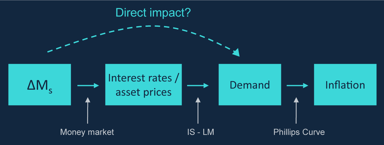
But the ‘monetarists’ raised a deeper objection—and it concerned precisely this assumption that an increase in the supply of money worked only by lowering the level of interest rates. They argued that it could also affect spending more directly. In essence, if one is at least to preserve the language of the model, their point was that a rise in the supply of money—broad money at least—shifts not just the ‘LM’ curve to the right but the ‘IS’ curve as well (chart 8).

Chart 8.

Monetarists argued that money affected spending directly, not just via interest rates and asset prices

Imagine something like Friedman’s ‘helicopter drop’—a sudden, windfall addition to everyone’s bank account. On its own, if nothing else happened, this would push up household wealth (the ‘W’ term in (1)). So even the conventional IS curve says, the result would be stronger demand. But let us suppose the ‘drop’ is financed by a tax on other, non-monetary assets, leaving household wealth in aggregate (the ‘W’ term) unchanged. Because people’s financial positions differ, partly by age—older people tend to have higher net wealth than younger people—this pair of transactions redistributes resources, away from long-term savers and towards borrowers. And if the latter group is ‘credit-constrained’—if they would like to spend and borrow more at the prevailing level of interest rates but, perhaps for want of collateral, cannot do so—then this transfer should boost demand. Net payers of the tax will cut back on their spending by less than the increase in demand from beneficiaries of the policy. Even when offset by an equal and opposite tax, and even for given interest rates, this addition of liquid assets would add to demand and inflation.

To me, this sounds perfectly plausible. Indeed, the MPC has often argued that these constraints can matter for the transmission of more standard changes in interest rates. If borrowers are (on average) more credit-constrained than savers, and therefore more sensitive to changes in cash flow, equal declines in debt interest costs on the one hand, and deposit receipts on the other, will on balance be expansionary.

Nor is this the only way in which a ‘helicopter drop’ might matter. The deeper point is that, if the very existence of money is accounted for by the presence of various financial frictions (i.e. departures from Hahn’s Arrow-Debreu world), then supplying more of it might plausibly ease these constraints. Conceivably, this could boost spending even without any change in bond yields or the prices of other assets.

If for no other, this is one reason why policymakers should always pay attention to the behaviour of the monetary aggregates. One should not presume that an IS relationship (based on something like (1)) always captures fully the degree of inflationary pressure in the economy or the transmission of monetary policy.

5. Stronger claims about quantities not borne out by the evidence

Equally, one cannot conclude either that these aggregates are the only thing you need to consider. Nor should one imagine—this was an approximation that both ‘Keynesians’ and ‘monetarists’ often seemed to make—that the one (broad money) is uniquely determined by the other (narrow money). Using recent experience in the UK, I want to discuss some of the challenges in interpreting these data.

Some, highlighted in the introduction, are evident in a simple split of the data over the inflation targeting period (for convenience, I have reproduced the relevant charts here). For the first 15 years of the current regime, from late 1992 until the beginning of the financial crisis in late 2007, there was very little growth of ‘narrow’ money (and none until reserve remuneration began in 2005), yet ‘broad’ money grew rapidly, by over 7½ per cent a year. By contrast, during the 10 years or so between the first use of QE in 2009 and the onset of the pandemic, central bank reserves rose very significantly, as one would have expected. Yet broad money growth slowed, to less than half the rate seen in those earlier, pre-crisis years. In terms of the money that really matters for the economy—deposits held by households and firms in commercial banks—its rate of creation has been much lower during QE than beforehand.

And over both periods, despite these gyrations in the respective measures of money growth, average CPI inflation was pretty much bang on 2 per cent.

What might explain this? How is it that the central bank’s balance sheet can expand so rapidly without a commensurate impact on those of commercial banks? And why, at least across these two periods, does neither measure of money growth seem to have much to do with inflation?

What follows is not remotely a full and comprehensive answer to these questions. Nor are the points made here remotely novel. Over the years, reams have been written about all of them, including in some very good articles by bank economists.Footnote ⁹ But they are certainly relevant in interpreting these data and therefore worth touching on.

One I mentioned in the introduction: commercial banks can create and withdraw deposits—principally in the act of extending or reducing the quantity of their lending—independently of their reserve holdings at the central bank. Suppose you borrow £100 from a bank. What the bank actually does, in granting the loan, is to put an extra £100 into your deposit account. This is newly created (broad) money, matched, on the asset side of its balance sheet, by the debt you now owe the bank. This process does not require any matching increase in reserves.Footnote ¹⁰

It has its limits, not least because banks are obliged to fund a proportion of their lending with equity (rather than deposits). They cannot (and do not) expand or reduce the quantity of money indefinitely. And monetary policy, via its effects on the wider economic environment, will also influence these decisions. But, if the suggestion in some of the simpler textbooks is that the central bank can control the size of commercial banks’ balance sheets as easily and directly as its own, this is clearly not the case. Influence is not control, and broad money certainly should not be considered an instrument of policy.

Second, and whatever the process by which their supply is determined, quantities of money—whether narrow or broad—can also be affected by changes in the demand for deposits. If the private sector wants to hold more of its wealth in this form, for a given level of spending and economic activity, then accommodating that demand has little effect.

And third, I think the experience of QE has shown pretty clearly that, at least when it comes to central bank reserves, it is not just the position of the M_D line that can change, but its slope as well. If so, and if you accept any part of the idea that injections of central bank money work via interest rates and asset prices, this means that a given quantity of QE can have differing effects on demand and inflation.

Let me start with the central bank’s balance sheet, taking the latter two points together. I will then circle back and discuss briefly the behaviour of the demand for broad money.

5.1. The demand for central bank money

In March 2020, when the world was struck by the pandemic, there were violent moves in prices of financial assets, volatility rose sharply and market liquidity—the preparedness of financial institutions to provide short-term credit—dried up. In order to meet margin calls on derivative positions, many investment firms were required to sell even safe assets (government debt). Whatever the underlying vulnerabilities that fed it, this ‘dash for cash’ can be thought of in this context as a sharp increase in the demand for central bank moneyFootnote ¹¹—in chart 9, a rightwards shift in the M_D line. Though the particular circumstances were different each time, I think you can characterise the conditions in early 2009, and again during the LDI crisis last October, in a similar manner.

Chart 9.

Unless accommodated and matched by greater supply a rise in the demand for money is contractionary

Note: (r’ _eq) shows the increase in the interest rate if the higher demand for money had not been accommodated by an increase in money supply.

Meeting such demand—matching the rightwards jump in M_D with a similar shift in M_S—is not monetary easing: it is the forestalling of a market-induced tightening of monetary conditions. Without that matching supply, bond yields would rise, asset prices would fall and aggregate demand and inflation would weaken (in the IS-LM model, an unmet rise in the demand for money pushes the ‘LM’ curve to the left). And it is one reason why, in the data, you would expect—at least occasionally—to see shifts in central bank money that are not then followed by stronger demand and inflation.Footnote ¹² It also suggests that, rather than just their size, a more accurate measure of the impact of asset purchases is what they do to bond yields. Combined, and by design, the dual shifts in chart 9 would leave those yields unchanged.

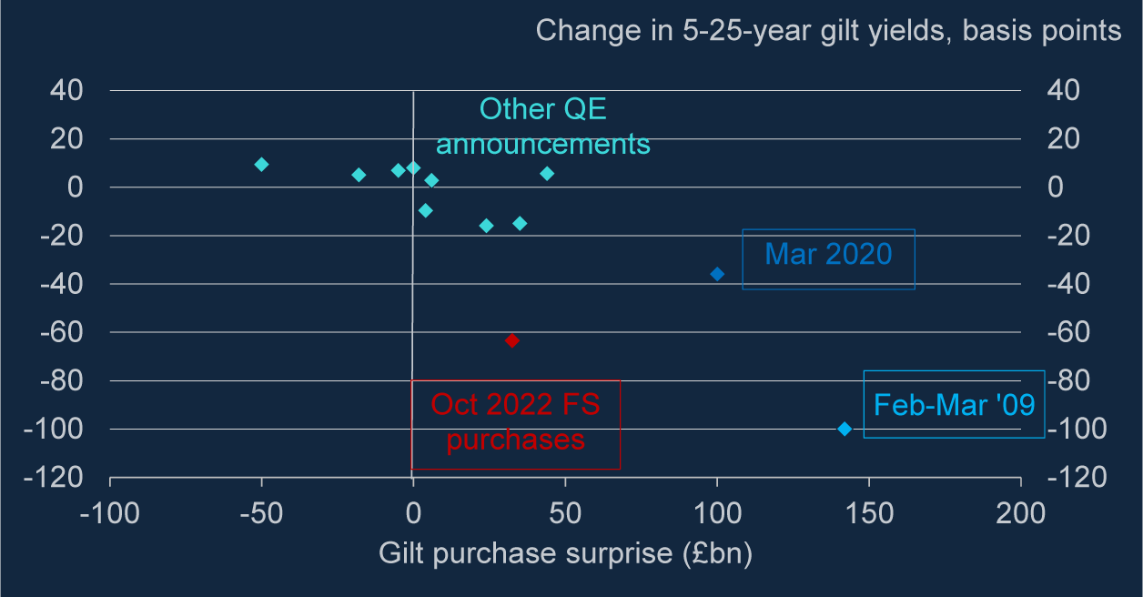
This conclusion is all the stronger once you recognise—as seems to be the case in the data—that the M_D line is subject to shifts not just to its position but also in its slope. The effects on bond yields of a given quantum of asset purchases appear to vary. In particular, it seems to be exactly during these episodes of acute market illiquidity—the three I singled out are circled in chart 10—that these purchases seem to have been the most effective at tempering any rise in yields.

Chart 10.

Asset purchases seem to have larger effects when markets are illiquid

Note: Chart shows the change in 5–25 year gilt yields, averaged across maturities, over two-day windows around announcements (see Joyce et al., Reference Joyce, Lasaosa, Stevens and Tong2011), except when there are confounding events within this window. October 2011, February 2012 and March 2020 use a narrower window, as MPC announcements coincided with other central bank announcements or major political news. Purchase surprise is the change in the expected target stock of QE purchases among market participants surveyed by Reuters (QE1–QE4) and market intelligence (QE5). Purchase surprise in the 28 Sep–14 Oct 2022 financial stability (FS) intervention is assumed to be £32.5 bn, the mean of a uniform distribution of purchase expectations based on the announced £65 bn ceiling.

Source: Bloomberg Finance L.P, Refinitiv Eikon, Reuters and Bank of England calculations.

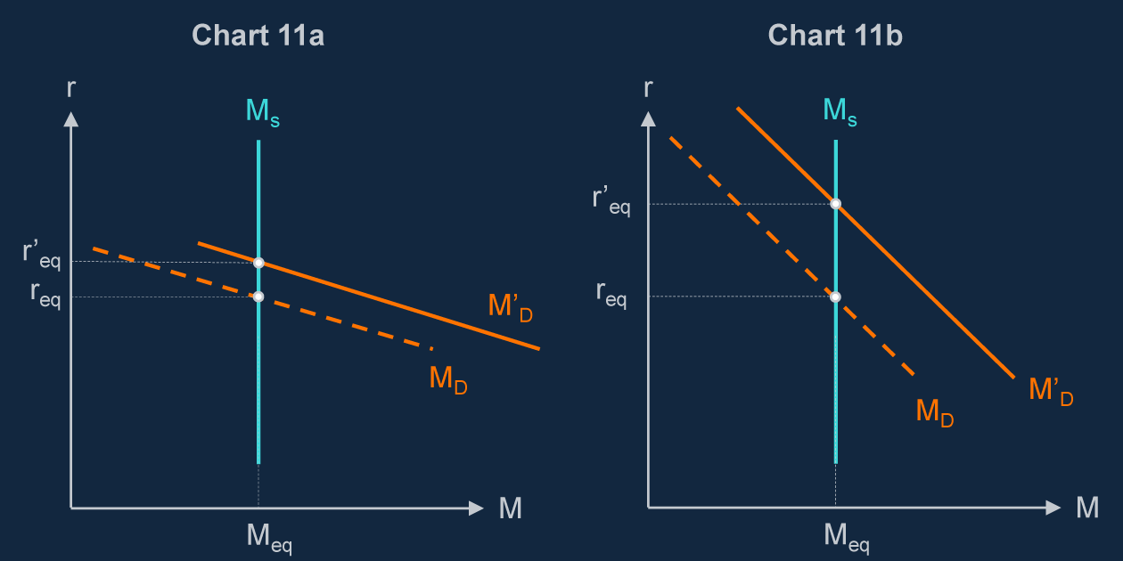
In liquid markets, the M_D line looks to be less steep. As I said earlier, the fact that central banks now pay interest on reserves will surely have tilted it in that direction. At least in normal times, there is arguably less difference, as far as the private sector is concerned, between a deposit in the central bank and (say) a short-term public debt instrument such as a Treasury bill. If repo markets are working smoothly, financial institutions can use even longer-term government debt to raise cash. This increases the degree of substitutability between the two sides of the QE transaction and has the effect of flattening the M_D curve.

Conversely, bouts of illiquidity are characterised by a lower degree of substitutability—relative to government debt, the distinctive liquidity value of money becomes more pronounced—and, as well as moving to the right, the M_D line steepens (chart 11).

Chart 11.

Money demand schedule is steeper when markets are less liquid

The MPC has often pointed out that QE seems to have had differing effects, according to economic and financial circumstances (they are ‘state-contingent’Footnote ¹³). The implication, as my colleague Silvana Tenreyro emphasised in a recent speech,Footnote ¹⁴ is that it makes more sense to think of the impact of the policy through the lens of prices—what it does to bond yields—than quantities.

This was also the recommendation of the Bank’s Independent Evaluation Office in a report issued a couple of years ago:

Rather than explaining QE in terms of ‘injecting’ or ‘printing’ money, QE could be framed as a continuation of conventional monetary policy that pushes down long-term interest rates … Framing QE as a change in an interest rate rather than the creation of a quantity of money may also reduce the perception that QE is a transfer of wealth to the rich or to banks.

I think this makes a good deal of sense.

5.2. The demand for commercial bank money

If desired holdings of central bank money can move around (even for given levels of aggregate spending and economic activity), the same appears to be true of commercial bank deposits. As we have seen, the supply processes need not be the same: in the case of broad money, it is usually the commercial banks themselves (not the central bank) that directly create the deposits, and effectively accommodate such shifts in demand.Footnote ¹⁵ But the basic intuition is the same. If the private sector wants to hold more in their bank accounts for a given level of spending—if the extra deposits are held not as a ‘medium of exchange’ but as a ‘store of wealth’—this need not have any implications for inflation.

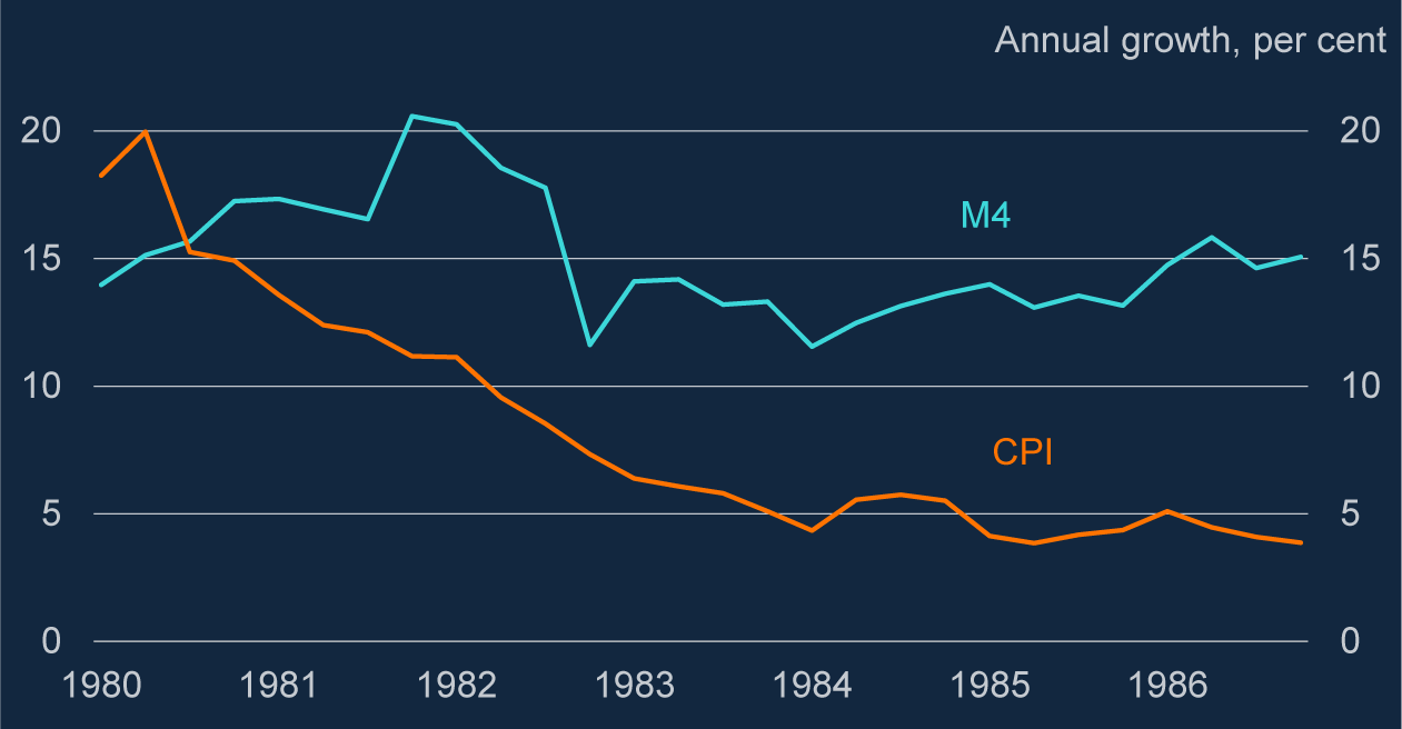
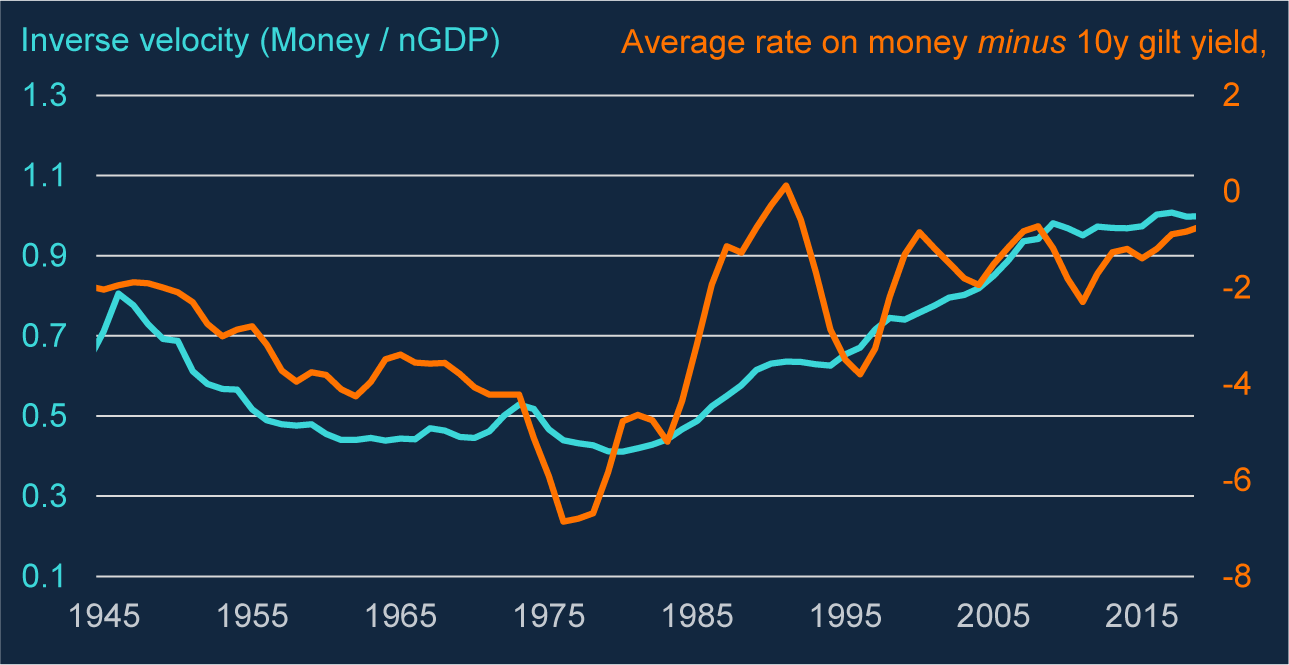
One clear example is the experience of the first few years of the 1980s. After years or extremely high inflation, the incoming UK government—which in those days set monetary as well as fiscal policy—was determined to reduce it. To this end, it set itself intermediate targets for broad money growth. These were repeatedly overshot—as you can see from chart 12, broad money growth remained stubbornly high—and eventually abandoned. Yet inflation fell sharply anyway.

Chart 12.

During the first half of the 1980s, broad money growth remained very high but inflation declined anyway

Source: ONS, Bank of England and Bank calculations.

At least with the benefit of hindsight, one can see that these differing trends reflected strong growth in the demand for money, alongside stronger supply. After the financial liberalisation of the early 1980s, banks had started to pay interest on deposit accounts, making them more competitive relative to securities like gilts (the orange line in chart 13 plots the spread between the two). So, it would make sense if the private sector wanted to allocate more of its financial assets to deposits. Because they were held as stores of value, these extra deposits were not inflationary.

Chart 13.

Demand for broad money increased from the 1980s as banks started paying interest on deposits

Note: Broad money is defined as M4ex from 1997, projected backwards with official data for M4 to 1963 and estimates from Thomas and Dimsdale’s Millennium of UK data (2017) to 1945, based on Capie and Webber (Reference Capie and Webber1985) and Sheppard (Reference Sheppard1971), and digitised here (https://www.escoe.ac.uk/research/historical-data/money-banking-and-credit/). Inverse velocity is defined as the stock of M4ex divided by annual nominal GDP. The rate of interest on broad money is a stock-weighted average of interest rates across the sectoral components of M4. These are based on annual averages of Divisia rates of return back to 1977. Prior to this they are based on data from Thomas and Dimsdale (2017) derived in part from estimates by Capie and Billings ( Reference Capie and Billings 2004 ).

Source: ONS, Bank of England, Thomas and Dimsdale (Reference Thomas and Dimsdale2017), Building Societies Association Year Books and Bank calculations.

As you see from chart 13—the blue line plots the ratio of broad money to nominal GDP—this trend continued for many years afterwards, including through the first 15 years of the inflation targeting era.Footnote ¹⁶

It may be that, in the latter part of this period, the very rapid growth of banks’ balance sheets—which was even more marked if you include their overseas balance sheets—was telling us something about the build-up of risks in the banking system. Financial crises are often preceded by rapid growth in measures of credit and, as we now know, that 2004–2007 period saw a significant worsening in the quality of banks’ assets and, on the liabilities side of their balance sheets, a sharp fall too in the share of loss-absorbing equity that funded them.

For my part, I am sceptical that higher interest rates would have done much to stem this. Nor, of course, did (or does) the MPC have a FS objective. What is clear is that rapid growth of broad money over that period did not cause or presage rapid inflation. To have succumbed to too crude, an interpretation of the monetary aggregates, by tightening policy aggressively in response to strong M4 growth, would have led to a material undershooting of the inflation target. Rightly, that was not the view taken by the MPC at the time.

This long expansion in bank deposits, relative to GDP, ended at around the time of the financial crisis. Changes in the structure of the financial system—in particular the partial shift away from bank lending and towards non-bank finance—may have had something to do with this. More fundamentally, the spread between interest rates on deposits and yields on competing securities became more stable. In addition, underlying growth in productivity and economic activity also slowed notably. All these things combined to slow the rate of growth of broad money, notwithstanding the rapid expansion of the central bank’s balance sheet.

6. The rise in broad money during the pandemic and the current inflation

So, the lesson of history is that most movements in broad money occur independently of variations in the size of the central bank’s balance sheet. Nor are many of them driven by exogenous changes in supply with no accompanying shift in the demand for money. They are not necessarily Friedman’s ‘helicopter drops’ and accommodating them need not have any implications for asset prices or for demand.

However, there may be times at which this is the more appropriate description. Arguably, the significant growth of M4 during the pandemic—and specifically the build-up of money in households’ bank accounts—counts as one such episode. Unable to spend during the lockdowns, but still receiving income (in part thanks to the government’s furlough scheme) households accumulated significant ‘excess deposits’ (chart 3). This was surely involuntary (hence the word ‘excess’) and was always likely to support the recovery of consumer spending once lockdowns were lifted.

And monetary authorities—including the MPC—treated this issue very much through this somewhat ‘monetarist’ lens. There was every reason to expect a strong recovery anyway, whatever the form of that additional wealth. As we emerged from the last lockdown in the spring of 2021, the level of consumer spending was still extremely low and, given the additional impetus provided by the rise in ‘W’, even equation (1)), which makes no distinction between monetary and non-monetary assets, would have predicted a very rapid bounce-back. But we certainly asked ourselves whether that would be all the stronger because of the liquid nature of this extra wealth.

Asking the question is one thing, answering it accurately another. It is obviously possible that we got that judgement wrong and under-estimated the significance of these extra deposits. However, in my view it is quite hard to argue that this could account for much of the subsequent upside surprise in inflation.

First, consumption growth—and that of aggregate demand—turned out to be weaker, not stronger, than the MPC (and many other forecasters) had anticipated. It was also weaker than the prediction of a simple, money-driven model. The orange line in chart 4 (reprinted from the introduction) plots the forecast values of an empirical ‘consumption function’, estimated on data up to the end of 2019, that looks a bit like equation (1)) but includes an additional term in household deposits (effectively splitting the ‘W’ term into monetary and non-monetary assets). In principle, this would allow for any additional impetus provided by the liquid nature of the extra wealth that households had accumulated during the pandemic. Yet the MPC’s forecast in the May 2021 Monetary Policy Report was stronger than this model’s prediction. And the actual out-turn was weaker than both. This might be for any number of reasons. One thing that might help to explain the shortfall is that the ‘excess deposits’ seemed to be skewed towards those—older and better-off households—less likely to be credit-constrained.

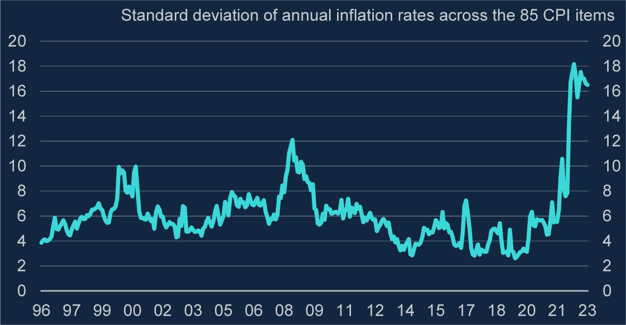
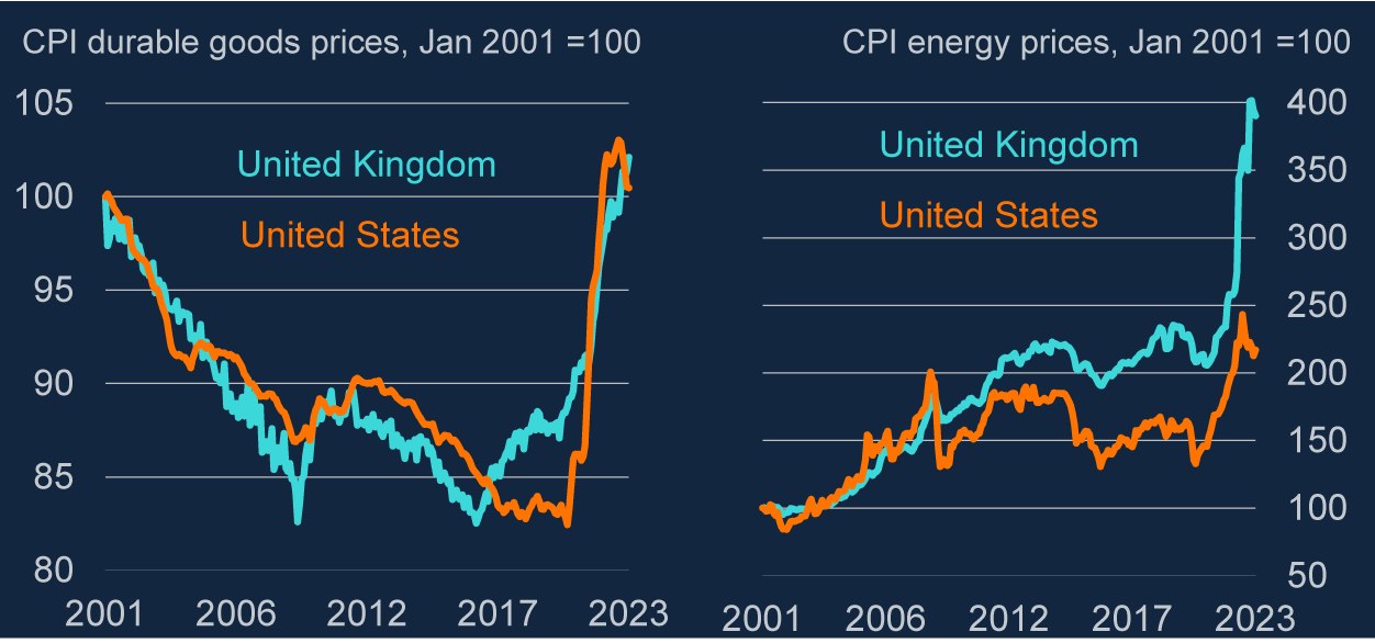
Second, inflation driven purely by a monetary expansion might be expected to raise all prices equally. That is very clearly not what has happened over the past couple of years. As chart 14 illustrates, there have been huge variations in relative prices—some have risen much faster than others. In 2021, the inflation was most marked in prices of core traded goods. In 2022 the big jumps were in energy and food prices (chart 15).

Chart 14.

Big shifts in relative prices since the pandemic

Source: ONS and Bank calculations.

Chart 15.

Large increase in global prices of durable goods in 2021, then those of energy (especially in Europe) in 2022

Source: ONS, FRED and Bank calculations.

Furthermore, one can readily identify things that account for this pattern. The pandemic caused a big shift in global consumer demand towards goods (and away from services) while at the same time impairing their supply. Although the resulting impact on core goods prices began to fade through the second half of last year it was then supplanted—and superseded—by the effects of the war in Ukraine on the supply and prices of food and energy. And the huge squeeze in real incomes, resulting from these jumps in import prices, has subsequently led to second-round effects on domestic wages and prices. This, to me, sounds the more plausible explanation of the data we have seen.

What would have been needed to control inflation? It is, of course, possible—with the benefit of hindsight—to imagine a different path for monetary policy over the past that would have kept inflation close to target even in the face of these subsequent shocks.

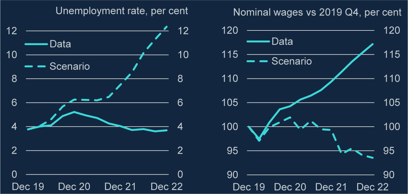
Using the Bank’s economic model, chart 16 plots the paths of unemployment and nominal wages necessary to keep price inflation roughly at 2 per cent through 2021 and 2022. The simulation suggests that interest rates would have to have risen well into double digits. Another thing it makes clear is that, as I argued in a talk last autumn,Footnote ¹⁷ there is no getting round the impact on real incomes of these jumps in import prices. One way or the other—whether as higher price inflation or lower wage inflation—increases on this scale are bound to result in a period of falling real pay (and also falling real profits for domestic companies). They inevitably reduce real national income.

Chart 16.

Monetary policy cannot offset the fall in real incomes caused by a terms of trade shock

Note: Nominal wages in the chart are private sector regular pay.

Source: ONS, Bank of England, Bloomberg Finance L.P. and Bank calculations.

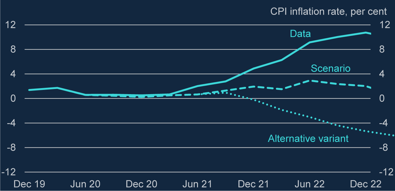
It is interesting too to ask what the world might now look like had this very steep path for interest rates been taken—but without any subsequent rise in import prices. The outcome of this experiment is the ‘alternative variant’ line in chart 17. The predicted result—this despite the prior growth in household deposits—is a steep fall in inflation, well into negative territory.

Chart 17.

In the absence of big rises in import prices, tighter policy would have pushed inflation into negative territory

Note: The ‘alternative variant’ reflects the same monetary tightening imparted in the ‘scenario’ but no increase in the contribution of import prices (energy and other goods) to CPI inflation relative to its pre-COVID average.

Source: ONS, Bank of England, Bloomberg Finance L.P. and Bank calculations.

All this makes it a challenge, I think, to argue that the rise in broad money in 2020 is the main (or even an important) contributor to the inflation that has followed.

7. QT and the MPC’s forecasts

I want to turn now to the second question I posed at the beginning: should the MPC not recognise in its forecasts some particular and additional drag on demand and on inflation, on top of that induced by higher Bank Rate, from the ongoing ‘quantitative tightening’ (or ‘QT’)? This began over a year ago, initially by failing to replace maturing gilts in the APF. In September, the MPC commenced outright sales of assets and said that, by both means, it would reduce its size by £80bn over the following year.

Readers who have come this far will be glad to hear that this section will be pretty brief because I have actually gone through the main points already. There are two. First, because the impact of QE has been variable, I do not think it would be right to pretend there is some fixed, unchanging effect on the economy—to translate, for example, a given quantity of asset purchases (or sales) into some notional equivalent in terms of Bank Rate. It is partly because of this, and the fact that we can only be less sure of its impact than that of conventional policy, that the MPC views Bank Rate as its ‘primary’ policy instrument. By design, the Committee did not embark on QT until the official interest rate reached a certain threshold—a level from which (were the need to arise) it could then be cut. It also said that, rather than responding to economic conditions—that is the task of the ‘primary’ instrument—the path of the APF would be ‘gradual and predictable’.

Second, and because of this, it is reasonable to suppose that this path is already reflected in the asset prices on which the MPC conditions its forecast. I have tried to argue today that the effects of QE and QT are transmitted predominantly via their impact on bond yields. The same goes for the expected path of the APF over the future: only surprises in QT decisions have an impact on these prices. So as long as there are no surprises—as long as the MPC always announces in advance its intentions, and the evolution of the balance sheet really is ‘predictable’—then the effects of QT will already be embodied in the yield curve. To add something else would be to double-count those effects.

8. Summary and conclusion

No monetary policymaker should ignore information that is relevant for future inflation. That includes the monetary aggregates.

But like most economic data, they need interpretation. Certainly, the very strongest claims—that QE inevitably leads to rapid growth of commercial bank deposits (M4), on a par with that in the central bank’s balance sheet; and that this, in turn, inevitably leads to excessive inflation—are not well supported by the evidence. Broad money grew more than twice as rapidly in the first 15 years of inflation targeting (when there was no QE) than in the decade or so after the financial crisis (when there was lots). And average inflation, in both periods, was close to 2 per cent.

This definitely does not mean that these indicators are somehow intrinsically unhelpful or misleading. Apart from anything else—and this is a more general point, relevant for other variables too—the act of targeting inflation is likely to reduce its correlation with just about every leading indicator (those things, at least, to which policy has a chance to react, given the lags involved). There might be several indicators that would have told you something about future inflation had monetary policy failed to react to them. But because in practice policy does just that, using and then offsetting that information, what has left will inevitably be less well correlatedFootnote ¹⁸ with inflation.

In the case of broad money, and at least with the benefit of hindsight, it is not that difficult to explain ‘what has left’ in these historical data. For a long period of time, right the way through from the early 1980s to the financial crisis over a quarter of a century later, household wealth rose (relative to income) and, because banks increasingly paid interest on their deposits, it became increasingly attractive to hold financial assets in that form. As a result, the demand for (broad) money rose alongside its rising supply—‘velocity’ declined, if you prefer—and the rate of M4 growth consistent with on-target inflation was significantly higher than 2 per cent. These were deposits accumulated not as a ‘medium of exchange’ but as a ‘store of wealth’.

What those years also demonstrate is that commercial banks can supply and create such deposits without any commensurate growth in the balance sheet of the central bank. QE is neither necessary nor sufficient for broad money to expand. To take a more recent example, it is not clear that the jump in household deposits during the pandemic was the direct and inevitable result of the central bank’s asset purchases at that time. If that were true, one would presumably have expected to see something similar after every other previous episode of asset purchases. That is not the case. For me, the more plausible cause is the combined impact of severe restrictions on spending and, thanks in part to fiscal support (in the shape of the furlough scheme), continuing growth in household income. At least in the first instance, the resulting jump in saving had nowhere to go but into household deposits.

More generally I think it is better to understand the impact of QE through the lens of asset prices—what it does to bond yields—than quantities (still less as ‘printing money’). As with commercial banks, the demand for central bank money can change (sometimes very abruptly). Furthermore, the response of yields to a given quantum of asset purchases seems to vary. There are times—particularly in periods of stress in financial markets—when government debt is viewed in markets as a relatively poor substitute for central bank money, and QE is therefore more powerful. At other times, it is less so.

If you also believe that markets (and therefore market prices) embody any impact of QE or QT expected to occur over the future, a forecast conditioned on those prices will also capture its effects. This is why it would not make sense, I think, to include in the MPC’s forecasts some separate and additional drag from the ongoing (and pre-announced) QT. That would be to double-count its impact.

All this said, there will certainly be times when movements in broad money are identifiably more supply- than demand-led. The jump in household deposits during the pandemic may not have been the inevitable result of QE but, from the perspective of households, it certainly looks like a windfall addition to their money holdings (i.e. something closer to Friedman’s ‘helicopter drop’). One might have expected an extra boost to spending whatever the form of these additional assets. But the MPC certainly allowed for a somewhat larger effect because of their liquid nature.

In the event, that forecast was too strong. Even before the squeeze on real incomes from the subsequent jumps in import prices, consumer (and aggregate) demand was weaker through 2021 than the MPC projected. That might have been for any number of reasons. One contributory factor may have been that the additional deposits were held disproportionately by people less likely to be ‘liquidity-constrained’—older and better-off households—and therefore less likely to spend them. (The very existence of money probably reflects financial frictions of this sort. It would not therefore be surprising if the distribution of a monetary ‘windfall’, across a diverse population, had some bearing on its effects.) Whatever the reason, this makes it difficult to see these additional deposits as the principal cause of the inflation that has followed. It is precisely those subsequent (and very large) jumps in import prices, and their second-round effects, that seem the more likely cause. This explanation would also accord much better with the very large changes we have seen in relative prices.

Finally, let me end with a more open question, one that is more about the future than the past. I’ve not addressed this directly today but it is certainly relevant. As chart 3 illustrates, household deposits (and aggregate M4) have actually been declining for some time since mid-2021, relative to household income.

The levels of these aggregates, on the other hand, are still higher than in the pre-pandemic period. Which of these matters more—a still-high level but a negative growth rate—depends a bit on your view of how households behave and how their demand for money is determined.

On one view (the ‘buffer stock’ approach), people are relatively tolerant of small variations in their money holdings and respond—whether by spending more on goods and services, buying other financial assets or paying down debt—only once deposits hit certain thresholds. If this is right, it is the level of money that matters and the fact that, on this measure, there still seem to be ‘excess’ deposits will continue to support consumer spending for a while yet. If, on the other hand, you believe that people respond more rapidly to an increase in the supply of money, the large accumulation of deposits during the pandemic is increasingly irrelevant and what matters more are the more recent, negative trends.

I am not sure if this is the critical judgement when it comes to our forecasts (it is certainly not the only thing affecting household behaviour). But it is, at least, illustrative of one point—that, as with just about every other economic indicator, changes in money holdings need some interpretation and their significance is not always 100 per cent obvious or ‘inevitable’.

Thank you.