


1. Introduction
Graphs can be used to represent geometric objects in 2D, 3D, or nD. For instance, a polygon soup is typically used in lighting simulation software for animated movies or video games. In topology-based geometric modeling, semantic information is added to the polygons to describe the topological relations between the object’s elements. For instance, the tabletop and the legs of a table are linked together. More precisely, topology-based geometric modeling deals with the representation and manipulation of objects according to their topological structure (cell subdivision in vertices, edges, faces, etc.) and their embedding (geometry and other types of information attached to their topological cells). Using the topological model of generalized maps (Damiand and Lienhardt Reference Damiand and Lienhardt2014; Lienhardt Reference Lienhardt1994), objects are defined as a particular subclass of labeled graphs. In generalized maps, arc labels encode the topological structure of the object while node labels store the embedding values. Defining embeddings on topological cells implies two facts. First, each node in the graph may have several embedding values. Secondly, all nodes that belong to the same cell must have the same embedding value. To satisfy these two properties, the model can store the embedding value either once per cell or once per node. In the first case, the object’s modifications rely on the possibility of efficiently retrieving these embedding values. In the second case, the application of a transformation operation can only be valid if it guarantees that all elements are adequately labeled, i.e., every node has a value for each embedding, and all nodes of a topological cell have the same value.
For instance, Figure 1A depicts the triangulation of a face and Figure 1B the removal of an edge, both in a colored 2D object. In either figure, the topological structure of the object contains four faces (two triangles, a square, and a pentagon) glued together, and the embedding associates a color to each face. Note that both operations simultaneously transform the topological structure and the embedding. The face triangulation topologically subdivides the face into triangles. From the embedding point of view, the new faces’ colors are computed as the mix of the subdivided face color and the neighboring face color. Topologically, the edge removal merges two neighboring faces by removing the shared edge, while the embedding modification mixes the two original face colors. Note that, in the case of the edge deletion, if we simply modify the graph nodes that describe this edge, we would create a unique face with two colors. Thus, we need to propagate the local modification to the whole face. However, when we delete an edge, we cannot assume the topology of the adjacent faces. These faces could have 3, 4, or arbitrary many edges and vertices. Therefore, we need a framework that ensures the preservation of consistency on a global scale.
Two modeling operations.

Topology-based geometric modeling exploits mathematically well-defined structures to specify algorithms expressing modeling operations. Proofs of correctness for these algorithms have to be done manually (Damiand and Lienhardt Reference Damiand and Lienhardt2014) or with the help of a prover like Coq (Puitg and Dufourd Reference Puitg and Dufourd1998). Each new operation must be proven to preserve model consistency for such solutions. On the other hand, procedural modeling relies on a small set of elementary rules that are shown to be coherent. Any other transformation is decomposed in a sequence of elementary rules and therefore preserves the model’s consistency. In this case, the rules are tailored to the applicative domain and are not necessarily transposable to other domains. Capitalizing on both approaches, we propose a framework in which transformations can be expressed as rules that preserve the model consistency. Static analysis of the rules guarantees consistency preservation. Therefore, we only need to prove that the rule conditions do ensure the preservation of the model consistency.
As topological structures can be represented as a particular class of graphs, the use of graph transformations to define modeling operations has already been studied (Pascual et al. Reference Pascual, Le Gall, Arnould and Belhaouari2022; Poudret et al. Reference Poudret, Arnould, Comet and Le Gall2008; Smith et al. Reference Smith, Prusinkiewicz and Samavati2004; Spicher et al. Reference Spicher, Michel and Giavitto2010). Derived from string and tree rewriting techniques, this rule-based approach offers a natural way to describe complex transformations intuitively. Graph transformations have applications in many areas such as software engineering (Baresi and Heckel Reference Baresi and Heckel2004; Heckel and Taentzer Reference Heckel and Taentzer2020), concurrent and distributed systems (Ehrig et al. Reference Ehrig, Kreowski, Montanari and Rozenberg1999), database design (Gyssens et al. Reference Gyssens, Paredaens, van den Bussche and van Gucht1994), IT landscape modeling (Haeusler et al. Reference Haeusler, Trojer, Kessler, Farwick, Nowakowski and Breu2019) and in our case geometric modeling. Graph transformations mainly offer a sound framework to express the preservation of domain-specific properties. For our concerns, they provide a tool for constraint-preserving modeling operations. In Poudret et al. (Reference Poudret, Arnould, Comet and Le Gall2008), we introduced dedicated rule variables to handle the topological genericity of modeling operations generically. These variables abstract topological cells and their transformations. To extend their usability, we showed that they offer a safer design of topological operations to produce a topological-based geometric modeler (Bellet et al. Reference Bellet, Poudret, Arnould, Fuchs and Le Gall2010), which was more accessible than traditional ad hoc implementations that are fastidious to code and vulnerable to consistency bugs. In Bellet et al. (Reference Bellet, Arnould and Le Gall2011), we defined a new graph category that allows nodes to have multiple labels in order to represent the multiple embedding types simultaneously (e.g., a face being labeled by both its color and its porosity). We proved the existence of graph transformations in this category and introduced a new type of dedicated variables and operators to express embedding transformations in rules.
In this article, we propose a generic graph transformation approach that allows the implementation of any application domain’s modeling operations. More precisely, this paper addresses the embedding aspect of modeling operations considering a representation of embedded generalized maps as labeled graphs introduced in Bellet et al. (Reference Bellet, Arnould and Le Gall2011) and in which node labels and associated labeling constraints encode the object embedding. Our first contribution is to give conditions on the relabeling graph transformations of Habel and Plump (Reference Habel and Plump2002) to guarantee the preservation of the embedding consistency. For example, in the case of the edge removal of Figure 1B, we will ensure that by construction, after the application of the corresponding rules, all nodes of the resulting face end up labeled with the same color. Our second contribution is the generic computation of the new embedding values created by a transformation. This generic computation is achieved with a rule-based language-based on Hoffmann (Reference Hoffmann2005). For instance, the mix of face colors for any colored object will be computable. The resulting rule schemes exploit dedicated graph transformation variables and terms to access the existing embedding through the topological structure and apply functions provided by the user with embedding data types. For example, the triangulation of Figure 1A will be defined by a rule scheme in which the colors of the created faces are computed by applying the user function “mix of two colors” to the subdivided face color and the respective adjacent face colors. The safety of this user-oriented language is as essential as its expressiveness. Therefore, our last contribution is providing syntactic conditions to guide rule scheme design and ensure the preservation of object consistency.
As a disclaimer, we wish to point out that we will refer to standard graph rewriting techniques, more precisely about versions of double-pushout rewriting. However, based on the specific needs of geometric modeling (e.g., orbit variables, computation of embedding values), the presented constructions will be a hand-curated version of DPO-rewriting exploiting element-based definitions to identify the various elements throughout the derivations. Essentially, we use inclusions instead of standard monomorphisms.
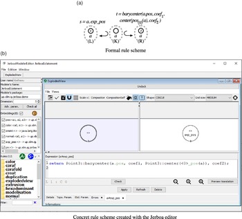
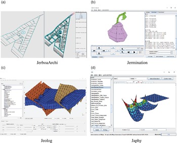
The remainder of this paper is structured as follows. First, Section 2 presents related works about L-system approaches of geometric modeling (usually referred to as procedural modeling) and some successful graph transformation applications. Sections 3 and 4 then present the theoretical foundations supporting our work. In Section 3, we describe relabeling in labeled graph transformations as introduced by Habel and Plump (Reference Habel and Plump2002) that will allow us to modify objects. We also present the use of variables in graph transformations as introduced by Hoffmann (Reference Hoffmann2005). The context of topological-based geometric modeling is then presented in Section 4. We focus on the topological model of generalized maps (Lienhardt Reference Lienhardt1994) and give conditions from Poudret et al. (Reference Poudret, Arnould, Comet and Le Gall2008) and Pascual et al. (Reference Pascual, Le Gall, Arnould and Belhaouari2022) to preserve the model consistency. Section 5 then similarly presents our embedded version of generalized maps and conditions under which graph transformations preserve the embedding consistency. The subsequent three sections focus on the rule-based language dedicated to embedding modifications. Section 6 introduces the rule scheme syntax, in particular terms that allow generic computation of new embedding values from existing ones in the object (e.g., to mix two unspecified face colors). Section 7 presents the rule scheme application, especially how schemes are instantiated to propagate minimally defined modifications (e.g., automatically change the color of all nodes of one face). Section 8 provides syntactic conditions on rule schemes to ensure embedding consistency preservation. This article presents the final version of the variables as they are implemented in the toolset Jerboa (Belhaouari et al. Reference Belhaouari, Arnould, Le Gall and Bellet2014) that allows the generation of a geometric modeler kernel from a set of rules. Some applications done with Jerboa are shown in Section 9, while concluding remarks are given in Section 10.
2. Related Work
This section presents the motivations and the origins of our graph transformation-based approach to geometric modeling.
Formal rule languages have been used for twenty-five years in the context of geometric modeling and are usually referred to as procedural modeling techniques. These techniques focus on creating a model from a rule set rather than editing the model via user input. They are particularly useful for modeling objects that are too cumbersome to be modeled by hand and for coping with the increasing level of details and size used to build complex and realistic objects.
Intuitively, a transformation rule looks like
 $A \rightarrow B$
and stands for the modification of object A into object B. This description of modifications within the object is highly visual and eases the design of geometric objects drastically. Indeed, this approach has been successfully applied to generate objects such as plants (Prusinkiewicz et al. Reference Prusinkiewicz, Lindenmayer and Hanan1988), terrains (see the survey done in Smelik et al. Reference Smelik, De Kraker, Tutenel, Bidarra and Groenewegen2009), buildings (Müller et al. Reference Müller, Wonka, Haegler, Ulmer and Van Gool2006) or cities (Parish and Müller Reference Parish and Müller2001).
In all these applications, object modifications are defined by a limited set of high-level operations such as creating a new branch, inserting a floor or subdividing a district with a road. Such operations do not contain all the low-level transformations on the actual object representation. Therefore, each high-level operation has its dedicated implementation and consistency preservation mechanism. This lack of adaptability entails that any change requires additional implementation and debugging efforts, which we avoid using graph transformations.
Graph transformations commonly refer to rule-based languages designed to manipulate graphs. The chosen framework for graph transformations is based on the definition of graphs and graph morphisms described using category theory. In that sense, graphs are defined by a set of objects, called nodes, and a set of links between these objects, called arcs. Among all graph transformation approaches, we choose the so-called double-pushout approach (or DPO) (Corradini et al. Reference Corradini, Montanari, Rossi, Ehrig, Heckel and Löwe1997; Ehrig et al. Reference Ehrig, Ehrig, Prange and Taentzer2006). We preferred double-pushout over single-pushout (or SPO) because in the SPO approach dangling edges after the deletion of the left-hand pattern are also deleted, which is less conservative. In other words, DPO eases the construction of conditions on rules to preserve constraints. The main drawback is having to check the dangling condition, which turns out to be doable in a static manner for our specific class of graphs, as shown in Poudret et al. (Reference Poudret, Arnould, Comet and Le Gall2008). Besides, we want to take advantage of the well-founded DPO framework given in Habel and Plump (Reference Habel and Plump2002), which allows the relabeling of nodes and arcs in graph transformations.
Habel and Plump (Reference Habel and Plump2001) showed that any computable function on graphs could be defined with a set of graph transformation rules supporting a non-deterministic application of rules, their composition and their iteration. However, in practical applications, operations are simpler to express and verify when defined as a single rule. Graph transformations have been enriched with variables to make them more generic while customizable to meet the various application needs. Intuitively, a rule with variables is a meta-level rule that yields a concrete rule for each possible instantiation of the variables with concrete elements. Different variable types have been introduced to enrich graph transformations depending on the genericity purposes : node replacement graph grammars (Engelfriet and Rozenberg Reference Engelfriet and Rozenberg1997) and hyperedge graph grammars (Drewes et al. Reference Drewes, Kreowski and Habel1997; Habel Reference Habel1992) somewhat generalized with cloning in adaptive star graph grammars (Drewes et al. Reference Drewes, Hoffmann, Janssens and Minas2010) or attribute graph grammars (Plump and Steinert Reference Plump and Steinert2004) and used for the interpretation of schematic diagrams (Bunke Reference Bunke1982) or image parsing (Han and Zhu Reference Han and Zhu2005).
Extensions made to graph transformations ease their integration in generic tools, such as GrGen.NET (Geiß et al. Reference Geiß, Batz, Grund, Hack and Szalkowski2006), (Groove Rensink Reference Rensink2004), AGG (Taentzer Reference Taentzer2004) or PROGRES (Schürr et al. Reference Schürr, Winter and Zündorf1995). Besides, graph transformations operate at a low level on graph structures. Thus, rules are self-contained. Therefore, a single rule application engine tailored to a given graph transformation class enables the application of all domain-related rules. These engines justifies the development of dedicated tools, such as Fujaba (Nickel et al. Reference Nickel, Niere and Zündorf2000) for code refactoring, (Gremlin Rodriguez Reference Rodriguez2015) for queries in graph databases, DiaGen (Minas and Viehstaedt Reference Minas and Viehstaedt1995) for the manipulation of diagrams, or GReTL (Ebert and Horn Reference Ebert and Horn2014) for the parallel construction of metamodels and conforming models. This point is crucial in designing a generic modeling tool as it minimizes the implementation and debugging efforts.
In computer graphics, graph transformations have already been used for several purposes. For instance, in You and Fu (Reference You and Fu1979), Tsai and Fu (Reference Tsai and Fu1980) attributed grammars were defined to describe and classify the syntactic structures of two-dimensional shapes. More recently, indoor scenes have been represented as graphs in Ikehata et al. (Reference Ikehata, Yang and Furukawa2015), where graph grammars allowed the reconstruction of scenes from images acquired by cameras. In Vilgertshofer and Borrmann (Reference Vilgertshofer and Borrmann2017), graphs describe the modeling process of tunnels, and graph transformations specify modifications to this process. The main idea is to handle consistency between different levels of detail in the infrastructure during transformations. In Ong and Kurth (Reference Ong and Kurth2012), multiscale modeling of plants also takes advantage of a graph grammar with the Relational Growth Grammar.
3. Graph Transformations
This section recalls the Double-PushOut (DPO) approach to graph transformations (Ehrig et al. Reference Ehrig, Ehrig, Prange and Taentzer2006), their specification in the category of partially labeled graphs (Habel and Plump Reference Habel and Plump2002) and their extension to rules with variables (Hoffmann Reference Hoffmann2005).
3.1 Double-pushout graph transformations
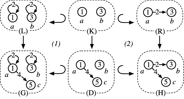
In the DPO approach, a transformation is expressed using two gluing diagrams defined in terms of category theory. More precisely, these diagrams are pushouts in the category of graphs and graph morphisms. To make the presentation more intuitive, let us consider the simple example of a DPO graph transformation given in Figure 2. The rule is given at the top of Figure 2 by the three graphs L, K, and R and by the two graph inclusions
Footnote 1
 $L \hookleftarrow K \hookrightarrow R$
where the symbol
 $\hookrightarrow$
(resp.
 $\hookleftarrow$
) denotes the inclusion when the source graph is given first (resp. secondly) and the target graph secondly (resp. first). In a rule, L is called the left-hand side, R the right-hand side, and K the interface of r. In this example, nodes are identified by letters (a, b or c) while arcs are anonymous. Nodes and arcs are labeled by numbers (1, 3, or 5 for the nodes and 2 or 4 for the arcs). Intuitively, the left-hand side of the rule L is the pattern to transform, the right-hand side R is the transformed pattern, and the interface K is the preserved part common to both L and R. The graph morphism
 $L \rightarrow G$
allows the matched pattern (graph L) to be identified inside the graph under modification (graph G). In Figure 2, the match morphism coincides with the inclusion.
DPO graph transformation.

In the first pushout (1), all elements (nodes and arcs) in L that are not in K are deleted from G to obtain D. In Figure 2, the two loops on nodes a and b are removed from L and thus are also removed in D. In the second pushout (2), elements in K are preserved while elements of R that are not already in K are added to D, yielding H. In Figure 2, an arc is added in the graph H between the two preserved nodes a and b. When the match morphism
 $m: L \rightarrow G$
meets some conditions,
Footnote 2
the double-pushout construction is well-defined and creates a unique graph H (up to graph isomorphism), that is the result of the application of the graph transformation
 $L \hookleftarrow K \hookrightarrow R$
through the match morphism
 $L \rightarrow G$
.
As already pointed out in Habel and Plump (Reference Habel and Plump2002), graph morphisms have to preserve arc and nodes labels, preventing relabeling in classical DPO transformation. Note that the relabeling of an arc can still be achieved by removing it while adding an arc with a new label between the same source and target nodes. However, this solution does not make the relabeling of a node possible. Consequently, we prefer the DPO approach of Habel and Plump (Reference Habel and Plump2002) that allows relabeling by considering partially labeled graphs. Let us take the example of the relabeling rule of Figure 3. Node b is labeled 7 in the left-hand side L and 3 in the right-hand side R, and therefore, it is unlabeled in the interface K. Note that the two morphisms
 $K \hookrightarrow L$
and
 $K \hookrightarrow R$
on partially labeled graphs L, K, R do not have to preserve labeling. In particular, the undefined label of b in K is not preserved.
A relabeling rule.

We now present the main definitions and results of Habel and Plump (Reference Habel and Plump2002) on partially labeled graph transformations.
3.2 Graph transformations on partially labeled graphs
A partially labeled graph
 $G = (V_G, E_G, s_G, t_G, l_{G,V}, l_{G,E})$
consists of two finite sets
 $V_G$
and
 $E_G$
of nodes and arcs, two source and target functions
 $s_G, t_G : E_G \rightarrow V_G$
, and two partial labeling functions
Footnote 3
 $l_{G,V} : V_G \rightarrow \mathcal{C}_V$
for the nodes and
 $l_{G,E} : E_G \rightarrow \mathcal{C}_E$
for the arcs, where
 $\mathcal{C}_V$
and
 $\mathcal{C}_E$
are fixed sets of node and arc labels. We say that G is totally labeled if
 $l_{G,V}$
and
 $l_{G,E}$
are total functions. A path in a graph G is a sequence
 $e_1...e_k$
of arcs from
 $E_G$
with
 $1 \leq k$
, such that
 $t_G(e_i)=s_G(e_{i+1})$
for each
 $1 \leq i < k$
.
 $s_G(e_1)$
and
 $t_G(e_k)$
are respectively called the path source and the path target, and the word
 $l_{G,E}(e_1)...l_{G,E}(e_k)$
is called the path label. Moreover, if
 $s_G(e_1)=t_G(e_k)$
, the path is called a cycle. Moving forward, we will amalgamate nodes and arcs in statements that hold for both sets by omitting the indices E and V for labeling functions
 $l_{G, V}$
and
 $l_{G, E}$
. In the sequel, partially labeled graphs will be simply called graphs.
A graph morphism
 $g : G \rightarrow H$
between two graphs G and H consists of
 $g_V : V_G \rightarrow V_H$
and
 $g_E : E_G \rightarrow E_H$
, two functions that preserve sources, targets and labels, i.e.,
 $s_H \circ g_E = g_V \circ s_G$
,
 $t_H \circ g_E = g_V \circ t_G$
, and
 $l_H(g(x)) = l_G(x)$
for all x in
 $Dom(l_G)$
. A morphism g is injective if
 $g_V$
and
 $g_E$
are injective and g is an inclusion if
 $g(x) = x$
for all x in G. In the latter case, the notation
 $ g : G \hookrightarrow H$
is preferred to
 $ g : G \rightarrow H$
. Finally, morphism composition is defined componentwise as function compositions.
A diagram of graph morphisms, as Figure 4A, is a pushout if (i)
 $K \rightarrow R \rightarrow H = K \rightarrow D \rightarrow H$
and (ii) for every pair of graph morphisms
 $(R \rightarrow H',~D \rightarrow H')$
with
 $K \rightarrow R \rightarrow H' = K \rightarrow D \rightarrow H'$
, there is a unique morphism
 $H \rightarrow H'$
such that
 $R \rightarrow H' = R \rightarrow H \rightarrow H'$
and
 $D \rightarrow H' = D \rightarrow H \rightarrow H'$
. The same diagram is a pullback if property (i) holds, and (iii) if for every pair of graph morphisms
 $(K' \rightarrow R,~K' \rightarrow D)$
with
 $K' \rightarrow R \rightarrow H = K' \rightarrow D \rightarrow H$
, there is a unique morphism
 $K' \rightarrow K$
such that
 $K' \rightarrow R = K' \rightarrow K \rightarrow R$
and
 $K' \rightarrow D = K' \rightarrow K \rightarrow D$
. A pushout is natural if it is also a pullback.
A diagram and a direct derivation.

Definition 1 (Rule). A rule
 $r : L \hookleftarrow K \hookrightarrow R$
consists of two inclusions
 $K \hookrightarrow L$
and
 $K \hookrightarrow R$
such that:
-
(1). for all
 $x \in L$
,
$l_L(x) = \bot$
implies
$x \in K$
and
$l_R(x) = \bot$
,
-
(2). for all
$x \in R$
,
$l_R(x) = \bot$
implies
$x \in K$
and
$l_L(x) = \bot$
.


Conditions (1) and (2) prevent invalid modifications of labels when the rule is matched to build a direct derivation.
Definition 2 (Direct derivation) A direct derivation from a graph G to a graph H via a rule
 $r : L \hookleftarrow K \hookrightarrow R$
consists of two natural pushouts as Figure 4B, where
 $m : L \rightarrow G$
, called the match morphism, is injective. We write
 $G \Rightarrow_{r,m} H$
if there exists such a direct derivation.
In Habel and Plump (Reference Habel and Plump2002), the authors studied the category of partially labeled graphs as a way to express relabeling in totally labeled graphs. In particular, given a rule
 $r : L \hookleftarrow K \hookrightarrow R$
and a match morphism
 $m: L \rightarrow G$
, they showed that (a) there exists a direct derivation
 $G \Rightarrow_{r,m} H$
as in Figure 4B if and only if m satisfies the following dangling condition: no node in
 $m(L) \backslash m(K)$
is incident to an arc in
 $G \backslash m(L)$
, (b) D and H are unique up to isomorphism, and (c) H is totally labeled if and only if G is totally labeled.
We consider rules with two inclusions for both sides (instead of only one for the left-hand side) as it yields a more conservative framework for us to express property preservation over direct derivations. Indeed, enforcing the morphism
 $K \hookrightarrow R$
to be an inclusion forbids that two nodes (resp. arcs) of L are transformed into a single node (resp. arc) in R.
We will use the following simplifications throughout the present article. First, spans of injective morphisms are considered spans of inclusions. Therefore, in a rule
 $r : L \hookleftarrow K \hookrightarrow R$
, if x is an element of K, we also write
 $x \in L$
and
 $x \in R$
. This simplification is extended through the diagram of a direct derivation. In other words, for a element x of D (in the diagram of Figure 4B), we also write
 $x \in G$
and
 $x \in H$
. Second, we do not extensively write morphisms but express them throughout node naming. For instance, a and b are node names in Figure 3. The morphism
 $K \rightarrow L$
maps the nodes a and b in the graph K to the nodes a and b in the graph L. Unless explicitly given, the depicted morphisms always map nodes with the same name. The arc part of the graph morphism is obtained by considering that the morphism is the maximal inclusion that respects node naming. When applying graph transformations on generalized maps, the adjacent arcs condition will ensure the uniqueness of arcs adjacent to node per dimension, unambiguously defining the arc part of the morphisms.
3.3 Graph transformations with variables
A framework for graph transformations with variables has been introduced in Hoffmann (Reference Hoffmann2005) revolving around three guidelines: the rule scheme syntax, the instantiation of variables, and the rule application process.
Rule scheme. The sets
 $\mathcal{C}_V$
and
 $\mathcal{C}_E$
of node and arc labels are extended by a set X of variable names. Graphs built over
Footnote 4
X are called graph schemes. Then, a rule scheme is a rule
 $r : L \hookleftarrow K \hookrightarrow R$
where L, K, and R are graph schemes. The kernel
 $\underline{G}$
of G is the graph obtained by removing all labels that contain a variable occurrence.
Instantiation. A substitution function
 $\sigma$
specifies how variable names occurring in a rule scheme are substituted. From the instantiation of variables in the graphs L, K, and R, yielding respectively the graphs
 $L_{\sigma}$
,
 $K_{\sigma,}$
and
 $R_{\sigma}$
, the instantiation of a rule scheme
 $r : L \hookleftarrow K \hookrightarrow R$
according to
 $\sigma$
defines a particular rule instance
 $r_\sigma : L_{\sigma} \hookleftarrow K_{\sigma} \hookrightarrow R_{\sigma}$
. Note that
 $r_\sigma$
is a rule without variables as defined in Definition 1.
Rule application. Let G be a graph, and
 $r : L \hookleftarrow K \hookrightarrow R$
be a rule scheme.
-
(1). Identify a kernel match
$\underline{m} : {\underline L} \rightarrow G$
of the kernel
${\underline L}$
of L in G (if it exists); -
(2). If possible, find a substitution
$\sigma$
such that there exists a morphism
$m : L_\sigma \rightarrow G$
extending
$\underline{m}$
; -
(3). Construct the instance
$r_\sigma : L_{\sigma} \hookleftarrow K_{\sigma} \hookrightarrow R_{\sigma}$
and apply the instance
$r_\sigma$
to get the direct derivation
$G \Rightarrow_{r_\sigma,m} H$
.


The substitution and the instantiation may differ depending on the variable type, but the generic framework remains valid. In Poudret et al. (Reference Poudret, Arnould, Comet and Le Gall2008) and Bellet et al. (Reference Bellet, Poudret, Arnould, Fuchs and Le Gall2010), we introduced variables that allow generic transformations of topological structures using this framework. However, neither of the previously defined variables exactly fits our usage: we need to access the node labels through the node names to allow topological structure traversals (e.g., to access the adjacent face color in the case of the colored triangulation given in the introduction). In the sequel, we will introduce new dedicated variables alongside a specific instantiation mechanism and ad hoc primitives for topological structure traversals.
3.4 Data types
In our setting, objects will be modeled by graphs labeled on nodes with geometric or dedicated data that we will generically call embedding. For the theoretical part of this paper, two examples of embeddings are considered, namely face colors and 2D positions of points, but Section 9 will present additional embeddings. These data are typed and provided with functions to perform computations on them.
As the same embedding value can appear multiple times in an object (e.g., in the transformed object of Figure 1, two faces have the same color), we need to identify these multiple occurrences when collecting object embedding values. We therefore consider for each data type
 $\tau$
, the type
 $\tau^\bullet$
, which corresponds to the multiset of elements of type
 $\tau$
. A multiset may be viewed as a function that associates its multiplicity (a natural number) to each element. We use the following notation:
 $[\![ ]\!]$
for the empty multiset (of any type
 $\tau^\bullet$
),
 $[\![ a_1,\ldots, a_p ]\!]$
for a multiset with p occurrences of elements of type
 $\tau$
. For example, the multiset that contains the element A with the multiplicity 1, the element B with the multiplicity 2, and where all other elements are of multiplicity 0, is
 $[\![ A,B,B ]\!]$
. Similarly, the multiset of face colors of the transformed object of Figure 1 is
 where each colored tablet directly encodes a particular color.
We then present the main elements of term construction and evaluation.
Signature. A data type signature
 $\Omega = (S,F)$
consists of a set S of type names and a family of function names provided with a profile on
 $\overline{S}$
with
 $\overline{S}$
defined as the set
 $S \cup \{ s^\bullet ~|~s \in S\}$
. A function name f provided with a profile
 $s_1 \ldots s_{m+1}$
with
 $s_i \in \overline{S}$
for
 $i \in 1..m+1$
is denoted by
 $f : s_1 \times \ldots \times s_m \rightarrow s_{m+1}$
.
Terms. For
 $X = \coprod_{s \in \overline{S}} X_s$
an
 $\overline{S}$
-indexed family of sets of variables, the set
 $ T_{\Omega}(X) = \coprod_{s \in \overline{S}} T_{\Omega}(X)_s$
of terms over
 $\Omega$
is the least set satisfying:
for all variables x in
$X_s$
,
$x \in T_{\Omega}(X)_s$
;for all function names
$f : s_1 \times \ldots \times s_m \rightarrow s_{m+1}$
in F, for all terms
$t_1 \in {T_{\Omega}(X)}_{s_1}$
,,
$t_m \in {T_{\Omega}(X)}_{s_m}$
, then
$f(t_1,\ldots,t_m) \in {T_{\Omega}(X)}_{s_{m+1}}$
.


We note
 $t:s$
a term t in
 ${T_{\Omega}(X)}_{s}$
.
Algebra. An
 $\Omega$
-algebra
 $\mathcal{A}$
consists of
an S-indexed family of nonempty sets
$\coprod_{s \in S} A_s$
, canonically extended with the family of sets
$\coprod_{s \in S} A_{s^\bullet}$
such that
\begin{equation*}A_{s^\bullet} = \{ [\![ a_1,\ldots,a_p ]\!] ~|~ 0 \leq p, \forall k \in 0..p, a_k \in A_{s} \}.\end{equation*}
and an F-indexed family of functions
$\coprod_{f \in F} f^A$
such that for each function
$f : s_1 \times \ldots \times s_m \rightarrow s_{m+1}$
in F, the function
$f^A$
has the profile
$f^A : A_{s_1} \times \ldots \times A_{s_m} \rightarrow A_{s_{m+1}}$
.


Evaluation. For
 $\sigma = \coprod_{s \in \overline{S}} \sigma_s $
an
 $\overline{S}$
-indexed family of assignments
 $\sigma_s : X_s \rightarrow A_s$
, the evaluation
 $\sigma: {T_{\Omega}(X)}_{s} \rightarrow A_s$
of a term
 $t:s$
is defined as:
for all variables x in
$X_s$
,
$\sigma(x) = \sigma_s(x)$
;for all function names
$f : s_1 \times \ldots \times s_m \rightarrow s_{m+1}$
in F and all terms
$t_1 : s_1$
,,
$t_m : s_m$
,
\begin{equation*}\sigma(f(t_1,\ldots,t_m)) = f^A(\sigma(t_1),\ldots,\sigma(t_m)).\end{equation*}


In order to design a modeler, the user is expected to provide both a data type signature
 $\Omega = (S, F)$
and an
 $\Omega$
-algebra
 $\mathcal{A}$
, with all the data types and functions required by its application domain to define its modeling operations. In the sequel, the considered user types are
 $point\_2D$
,
 $vector\_2D$
and color, that respectively model 2D positions, 2D vectors and colors. They are provided with all classical functions such as
-
$ + : point\_2D \times vector\_2D \rightarrow point\_2D$
that represents the translation of a point by a vector,
-
$midpoint : point\_2D \times point\_2D \rightarrow point\_2D$
that computes middle point of a line segment defined by its two endpoints,
-
$center : point\_2D^\bullet \rightarrow point\_2D$
that computes the barycenter of a multiset of points,
or
$mix : color \times color \rightarrow color$
that defines the average color of two given colors.


From now on, the algebra
 $\mathcal{A}$
will be left implicit. When needed, the carrier set
 $\mathcal{A}_{\tau}$
of a data type
 $\tau$
will be simply written
 $\lfloor \tau \rfloor$
.
By offering a concise and straightforward notation for multisets, our presentation of data types minimally meets our needs. Multiset properties such as commutativity of the element insertion or specification of the element multiplicity are semantically imposed. Note that multisets could also have been introduced by considering a higher-order approach as a starting point. We could have defined type constructions such as lists, sets, or tuples of elements of the same type. However, the resulting data types would have been more expressive than necessary, creating types such as sets of sets when we only need a generic construction for denoting multisets of basic type elements.
In the rest of the article, signatures introduced by the user will be called user signatures. As stated above, for the particular case of the example running throughout the paper, the user signature will contain the user types
 $point\_2D$
,
 $vector\_2D$
, and color.
4. Topological Generalized Maps as Partially Labeled Graphs
In topology-based modeling, objects are defined according to:
their topological structure – i.e., their cell subdivision (vertices, edges, faces, volumes) and the adjacency relations between these cells; for example, the three objects of Figure 5 have the same topological structure: a closed face F that has four edges and four vertices;
Figure 5.Objects of same topological structure.
their embedding, which includes all other types of information attached to their topological cells, including the geometric information required to capture their shape; for the objects of Figure 5, geometric points are attached to topological vertices, and colors are attached to faces.

Many topological structures allow one to represent different classes of objects: tetrahedral (Lang and Lienhardt Reference Lang and Lienhardt1996) or polyhedral (Damiand and Lienhardt Reference Damiand and Lienhardt2014; Mäntylä Reference Mäntylä1988; Weiler Reference Weiler1988), fixed dimension (2D Mäntylä Reference Mäntylä1988 or 3D Weiler Reference Weiler1988) or dimension-independent (Damiand and Lienhardt Reference Damiand and Lienhardt2014; Lang and Lienhardt Reference Lang and Lienhardt1996), and most of them can be seen as a particular class of graphs. Among those, we choose the topological model of generalized maps (or G-maps) (Damiand and Lienhardt Reference Damiand and Lienhardt2014; Lienhardt Reference Lienhardt1994) because its mathematical definition can be rather easily encoded within a formal framework. In G-maps, the topological structure is handled by both the graph structure and the arc labels, while the node labels define the embedding.
More precisely, the class of G-maps that represents valid objects is defined by labeling constraints. Hence, to define modeling operations with graph transformations, we investigate under which conditions G-map constraints and object consistency are preserved by transformations. Examples of inconsistencies are given in Figure 6. For instance, an edge with a single extremity instead of two or two faces glued along a vertex instead of an edge are topological inconsistencies (See Figure 6A). However, faces embedded with two colors instead of one or without any defined color are embedding inconsistencies (See Figure 6B).
Object inconsistencies.

4.1 Generalized maps
The representation of an object as a G-map intuitively comes from its decomposition into topological cells. For example, the 2D topological object of Figure 7A can be decomposed into a 2-dimensional G-map. First, the object is split into faces in Figure 7B. These faces are linked along their common edge with a 2-relation: the index 2 means that faces (cells of dimension 2) share a common edge. Similarly, faces are separated into edges connected with the 1-relation in Figure 7C. Finally, edges are divided into vertices by the 0-relation yielding the 2-G-map of Figure 7D. Nodes obtained at the end of the process are the G-map ones, and the different i-relations become labeled arcs: for a 2-dimensional G-map, labels i belong to
 $\{0,1,2\}$
. Let
 $G_{topo}$
be the 2-G-maps obtained from the decomposed of the topological object of Figure 7A and depicted in Figure 7E.
Topological decomposition of a geometric 2D object.

Therefore, G-maps are graphs labeled on the arcs by integers. More precisely, for a given dimension n, n-G-maps are graph with arcs totally labeled in
 $\mathcal{C}_E = 0..n$
, where
 $0..n$
is the interval of integers between 0 and n. Moreover, G-maps are symmetric graph: for each i-arc of source v and target v’, there is also a corresponding reversed i-arc of source v’ and target v. Graphically, double reversed arcs are represented with lines (see Figure 7E). Besides, instead of writing arc labels on the figures, we use the graphical codes introduced in Figure 7: black line for 0-arcs, red dashed line for 1-arcs, and blue double line for 2-arcs.
Topological cells are implicitly defined as subgraphs in G-maps. They are computed as all elements reachable from a source node using a given set of arc labels. For example, in Figure 8A, the 0-cell (vertex) adjacent to e is the subgraph which contains e, the nodes that can be reached from node e using 1-arcs or 2-arcs, and the arcs themselves. Note that the gray parts of the graphs in Figure 8 (later on in Figures 9 and 21) do not belong to the orbits and are only drawn to help with the visualization. In Figure 8B, the 1-cell adjacent to e (edge w in Figure 7A) is the subgraph that contains the node e and nodes reachable through 0-arcs and 2-arcs (nodes e, f, g, and h), and the corresponding arcs. Finally, in Figure 8C, the 2-cell adjacent to e (face
 $\mathcal{F}$
in Figure 7A) is the subgraph built from node e with 1-arcs and 2-arcs. The set of arc labels used to build the topological cell as subgraphs is called an orbit type.
Orbits adjacent to e.

Completions.

Definition 3 (Orbit type) Let
 $n \in \mathbb{N}$
be a dimension.
An orbit type of dimension n is a subset of
 $0..n$
, noted as a word o and placed in square brackets
 $\langle {o} \rangle$
. An element i of
 $0..n$
belongs to
 $\langle {o} \rangle$
if i occurs in o.
For instance, the orbit type
 $\{1,2\}$
can be noted indifferently
 $\langle {1~2} \rangle$
or
 $\langle {2~1} \rangle$
. In the sequel, the dimension of an orbit type is often left implicit.
Subgraphs built using graph traversals on an orbit type are called orbits. Formally, an orbit is an equivalence class for the equivalence relation defined by the corresponding orbit type. Based on this equivalence relation, we consider the notion of completion, which can be seen as the union of equivalence classes generated by a subgraph. The following definition formally introduces these notions together with topological graphs that include G-maps and their transformation patterns. Note that the arc labeling function of topological graphs is denoted by
 $\alpha$
according to the notation commonly used in geometric modeling.
Definition 4 (n-topological graph and orbit) Let
 $n \in \mathbb{N}$
be a dimension.
A partially labeled graph
 $G = (V, E, s, t, l_{V}, \alpha)$
is an n-dimensional topological graph if the arc labeling function
 $\alpha$
is a total function with codomain
 $\mathcal{C}_E=0..n$
.
For an orbit type
 $\langle {o} \rangle$
of dimension n, let
 $\equiv_{G\langle {o} \rangle}$
be the equivalence orbit relation defined on
 $V \times V$
as the reflexive, symmetric, and transitive closure built from arcs with labels in o, i.e., ensuring that for each arc e of G labeled by a letter in o, we have
 $s(e) \equiv_{G\langle {o} \rangle} t(e)$
.
For any node v of
 $G= (V,E,s,t,l_V,\alpha)$
, the
 $\langle {o} \rangle$
-orbit of G adjacent to v, denoted by
 ${G\langle {o} \rangle(v)}$
, is defined as the smallest subgraph
 $(V',E',s',t',l'_V,\alpha')$
of G such that
-
(1). the set V’ of nodes includes
$\{v\} \cup \{ v' ~|~ v' \in E, \; \exists w \in V', v' \equiv_{G\langle {o} \rangle} w \}$
, -
(2). the set E’ of arcs includes
$\{ e ~|~ s(e) \in V', \; t(e) \in V', \; \alpha(e) \in o \}$
, -
(3). and
$s',t',l'_V,$
and
$\alpha'$
are restrictions of corresponding functions in G to the sets V’ or E’.


If the context is clear,
 ${G\langle {o} \rangle(v)}$
is simply denoted
 $\langle {o} \rangle(v)$
.
More generally, for any subgraph
 $G' \hookrightarrow G$
, the
 $\langle {o} \rangle$
-completion of G’ in G, denoted by
 $G\langle {o} \rangle(G')$
, is defined as the smallest subgraph
 $(V'',E'',s'',t'',l''_V,\alpha'')$
of G such that
-
(1). the set V” of nodes includes
$V_{G'} \cup \{ v'' ~|~ v'' \in E, \; \exists w \in V'', v'' \equiv_{G\langle {o} \rangle} w \}$
, -
(2). the set E” of arcs includes
$\{ e ~|~ s(e) \in V'', \; t(e) \in V'', \; \alpha(e) \in o \}$
, -
(3). and
$s'',t'',l''_V,$
and
$\alpha''$
are restrictions of corresponding fonctions in G to the sets V” or E”.


The topological cells are particular instances of orbits. For instance, an orbit of type
 $\langle {0~1} \rangle$
is a face, an orbit of type
 $\langle {0~2} \rangle$
is an edge, and an orbit of type
 $\langle {1~2} \rangle$
is a vertex. Some other standard topological objects can be expressed as orbits. For example, the orbit
 $\langle {0} \rangle(e)$
in Figure 8D represents the half-edge (also called face edge) adjacent to e, and the orbit
 $\langle {0~1~2} \rangle(e)$
in Figure 8E represents the whole connected component.
Let us now take two examples to illustrate the notion of completion. The topological graph of Figure 9A is the
 $\langle {1~2} \rangle$
-completion of
 $\langle {0~2} \rangle (e)$
, i.e., the vertex completion of the edge adjacent to node e. The edge adjacent to node e, already shown in Figure 8B, is composed of the nodes e, f, g, and h with the 0-arcs and 2-arcs between them. The
 $\langle {1~2} \rangle$
-completion of this subgraph contains all nodes (and the corresponding arcs) reachable from e, f, g, or h through 1-arcs and 2-arcs. From the initial subgraph, nodes c, d, i, and j are added. Symmetrically, the Figure 9B presents the
 $\langle {0~2} \rangle$
-completion of the vertex
 $\langle {1~2} \rangle (e)$
. The vertex
 $\langle {1~2} \rangle (e)$
is illustrated on Figure 8A and the completion adds the nodes a, f, h, and k. Note that the notions of orbit equivalence and orbit completion will be helpful later in the article to handle embedding transformations.
Formally, a G-map is a topological graph satisfying some constraints that transcribe the object consistency. The constraints are the following.
Definition 5 (Generalized map) An n-dimensional generalized map, or n-G-map, is a totally labeled n-topological graph
 $G = (V, E, s, t, l_{V}, \alpha)$
that satisfies the following topological consistency constraints:
Symmetry constraint: G is symmetric,
Adjacent arc constraint: each node is the source node of exactly
$n+1$
arcs respectively labeled from 0 to n,Cycle constraint: for every i and j in
$0..n$
such that
${i+2 \leq j}$
, there exists a cycle labeled by ijij starting from each node.


These constraints ensure that objects represented by embedded G-maps are consistent manifolds (Lienhardt Reference Lienhardt1994). In particular, the cycle constraint ensures that in G-maps, two i-cells can only be adjacent along (
 ${i-1}$
)-cells. For instance, in the 2-G-map of Figure 7E, the 0 2 0 2-cycle constraint implies that faces are glued along topological edges. Let us notice that thanks to loops (see the 2-loops in Figure 7D), these three constraints also hold at the border of objects.
4.2 Basic topological transformations
Within a geometric modeler, operations defined on objects are called topological (resp. geometric) if their primary purpose is to change the topological structure (resp. the embedding). Operations may fall under both aspects, such as the rounding operation consisting of replacing a vertex or a sharp edge with a curved surface (Ledoux et al. Reference Ledoux, Arnould, Le Gall and Bertrand2002).
Intuitively, topological operations are applications that allow building new generalized maps from generalized maps. The definition of topological operations by graph transformation rules advantageously facilitates the study of stating whether or not the resulting graphs are also generalized maps. To achieve this, rules on generalized maps need to preserve the topological constraints of Definition 5 by construction.
In previous work (Poudret et al. Reference Poudret, Arnould, Comet and Le Gall2008), we elaborated the following syntactic conditions that precisely ensure the preservation of topological consistency:
Theorem (Topological consistency preservation) Let
 $r : L \hookleftarrow K \hookrightarrow R$
a graph transformation rule, G an n-G-map and
 $m:L \rightarrow G$
a match morphism.
The result H of the direct transformation
 $G \Rightarrow^{r,m} H$
is an n-G-map H if the following conditions of topological consistency preservation are satisfied:
-
Symmetry condition: the three graphs L, K, and R are symmetric n-topological graphs.
-
Adjacent arcs condition:
-
preserved nodes of K are sources of arcs having the same labels in both the left-hand side L and the right-hand side R;
-
removed nodes of
$L \backslash K$
and added nodes of
$R \backslash K$
must be source of exactly
$n+1$
arcs respectively labeled from 0 to n.
-
-
Cycle condition: for every i and j in
$0..n$
such that
${i+2 \leq j}$
, -
any added node of
$R \backslash K$
is the source of an ijij-cycle; -
any preserved node of K which is the source of an ijij-cycle in L, is also the source of an ijij-cycle in R;
-
any preserved node of K which is not the source of an ijij-cycle in L is source of the same i-arcs and j-arcs in L and R.


The interested reader can find some discussion on the conditions presented in this theorem in Poudret et al. (Reference Poudret, Arnould, Comet and Le Gall2008), with its proof. In particular, we demonstrated that the dangling condition (see Subsection 3.2) is always ensured when a rule that satisfies those conditions is applied to a G-map. Topological variables introduced in Poudret et al. (Reference Poudret, Arnould, Comet and Le Gall2008), Bellet et al. (Reference Bellet, Poudret, Arnould, Fuchs and Le Gall2010) and the corresponding rule schemes allow the abstraction of all orbits of a given type. Some syntactic conditions on the rule schemes were also given to ensure that instantiated rules satisfy the conditions of Theorem 4.2. These variables have been revisited with a functorial approach exploiting a product-based construction in Pascual et al. (Reference Pascual, Le Gall, Arnould and Belhaouari2022). Here we aim to discuss geometric operations, meaning that the embedding consistency is the issue tackled. Thus, the topological consistency will not be discussed more thoroughly, and we will use the more specific presentation of Poudret et al. (Reference Poudret, Arnould, Comet and Le Gall2008). Nonetheless, a watchful reader can notice that all the rules in this paper verify the constraints of Theorem 4.2, which guarantees that generalized maps remain generalized maps after transformations.
5. Embedded Generalized Maps and their Basic Transformations
Our approach is generic in the dimension of the objects and nature of the considered embedding. In the sequel,
 $n-G$
-maps will be called G-maps, and orbit type will implicitly be of dimension n. Moreover, all illustrative examples will present 2D objects with one of the two embedding data types of Figure 5: either 2D positions on vertices (i.e.,
 $\langle {1~2} \rangle$
-orbits) or colors on faces (i.e.,
 $\langle {0~1} \rangle$
-orbits).
5.1 Embedding representation
The topological structure of G-maps has been defined as graphs with arc labels. We complete this definition here with node labels to represent the embedding. In Section 3.4, we already sketched that every dedicated embedding has a data type and is defined on a particular kind of topological cell.
A node labeling function defining an embedding will be typed both by an orbit type and a data type. We characterize such a node labeling function as an embedding operation
 $\pi : \langle {o} \rangle \rightarrow \tau$
where
 $\pi$
is the operation name,
 $\tau$
is a data type, and
 $\langle {o} \rangle$
is an orbit type. Thus, for a G-map embedded on
 $\pi: \langle {o} \rangle \rightarrow \tau$
, the node label set
 $\mathcal{C}_{V}$
is the set of values
 $\lfloor \tau\rfloor$
of type
 $\tau$
. When the profile of
 $\pi$
is obvious, the node labeling function is noted
 $\pi$
. Therefore, an embedded
Footnote 5
G-map is a particular case of partially labeled graphs, generically denoted as a tuple
 $(V, E, s, t, \pi, \alpha)$
.
In this article, we consider the following embedding operations defined on the user signature introduced in Section 3.4 (i.e., including types
 $point\_2D$
and color):
-
$pos : \langle {1~2} \rangle \rightarrow point\_2D$
is the embedding that associates a 2D position to each vertex. Figure 10A shows the embedded G-map
$G_{pos} = (V,E,s,t,pos,\alpha)$
built on
$G_{topo}$
(see Figure 7D). The embedding operation pos maps the 2D positions A, B, C, D, and E to the nodes of V;Figure 10.
Two embedding operations.
-
$col : \langle {0~1} \rangle \rightarrow color$
is the embedding that associates a color (values of type color) to each face (
$\langle {0~1} \rangle$
-orbits) of a 2-G-map. Figure 10B illustrates the embedded G-map
$G_{col} = (V,E,s,t,col,\alpha)$
built on
$G_{topo}$
, thus sharing its topological elements with
$G_{pos}$
. The embedding operation col maps colors to the nodes of V.


 to the nodes of V.
As mentioned in Section 3.4, data types used to specify embedding come with operations to perform computations on the data. In the following, when referring to the user signature attached to a given embedding
 $\pi : \langle {o} \rangle \rightarrow \tau$
, we will generically note it as
 $\Omega_\pi = (S_\pi, F_\pi)$
. In particular,
 $S_\pi$
contains the type
 $\tau$
and
 $F_\pi$
contains functions defined on
 $\overline{S_\pi} = S_\pi \cup \{ s_\pi^\bullet ~|~ s_\pi \in S_\pi \}$
.
Moreover, as an embedding operation
 $\pi: \langle {o} \rangle \rightarrow \tau$
is characterized by its domain orbit, all nodes of a common
 $\langle {o} \rangle$
-orbit share the same label by
 $\pi$
, also called
 $\pi$
-label. For
 $G_{pos}$
of Figure 10A, as pos is defined on orbit type
 $\langle {1~2} \rangle$
characterizing vertices, all nodes of a same
 $\langle {1~2} \rangle$
-orbit have the same value by pos. Thus, nodes c, e, g, and i that belong to the same vertex orbit
 $\langle {1~2} \rangle$
are labeled by the same value B. Similarly, in Figure 10B, nodes a, b, c, d, e, and f that belong to the same face are labeled with the same yellow color. This property is captured by an embedding constraint (Bellet et al. Reference Bellet, Arnould and Le Gall2011):
Definition 6 (Embedded graph and embedded generalized map) Let
 $\pi : \langle {o} \rangle \rightarrow \tau$
be an embedding operation with
 $\langle {o} \rangle$
an orbit type and
 $\tau$
a data type.
Embedded graph: A graph embedded on
$\pi$
, or
$\pi$
-embedded graph, is an n-topological graph
$G = (V, E, s, t, \pi, \alpha)$
where
$\pi$
labels nodes on
$\mathcal{C}_{V} = \lfloor \tau \rfloor$
.Embedding consistency constraint: A
$\pi$
-embedded graph satisfies the embedding consistency constraint if for all nodes v and w such that
$v \equiv_{\langle {o} \rangle} w$
,
$\pi(v) \neq \bot$
and
$\pi(w) \neq \bot$
, then
$\pi(v) = \pi(w)$
.Embedded G-map: A
$\pi$
-embedded G-map is an n-G-map embedded on
$\pi$
satisfying the embedding consistency constraint and such that
$\pi$
is a total function (i.e.,
$Dom(\pi)=V$
).


Note that the embedding consistency constraint allows an
 $\langle {o} \rangle$
-orbit to be partially
 $\pi$
-labeled as long as the defined
 $\pi$
-labels are equal. Because embedded G-maps are totally labeled, the constraint entails that all nodes of a
 $\langle {o} \rangle$
-orbit share the same embedding value, i.e., for all nodes v and w such that
 $v \equiv_{\langle {o} \rangle} w$
,
 $\pi(v)=\pi(w)$
with
 $\pi(v) \neq \bot$
. Similar to the construction of the DPO approach to graph transformation in Habel and Plump (Reference Habel and Plump2002), we consider partially labeled objects in rules to ease the modification of totally labeled objects.
As we have already noticed with the embedded G-maps
 $G_{pos}$
and
 $G_{col}$
, the topological structure of a
 $\pi$
-embedded graph G can then be found by forgetting its node labels. For
 $G = (V, E, s, t, \pi, \alpha)$
,
 $G_\alpha = (V, E, s, t, \bot, \alpha)$
denotes the underlying topological structure where the everywhere undefined function
 $\bot$
replaces the node labeling function
 $\pi$
.
Given an equivalence relation
 $\equiv$
on a set X, [x] is the equivalence class of an element x of X, i.e.,
 $\{ y \in X ~|~ y \equiv x \}$
, whereas
 $X_{/ \equiv}$
is the quotient set
 $\{ [x] ~|~ x \in X \}$
. In a
 $\pi$
-embedded graph G, the relation
 $\equiv_{\langle {o} \rangle}$
defines a partition of the nodes if it satisfies the embedding consistency constraint. Consequently, the quotient of G by
 $\equiv_{\langle {o} \rangle}$
is well-defined and yields its
 $\langle {o} \rangle$
-orbits. In a G, all nodes of a
 $\langle {o} \rangle$
-orbit are unlabeled or share the same
 $\pi$
-label. Therefore, if this
 $\pi$
-label exists, it is directly inherited by the resulting quotient node. For the quotient set of arcs, we consider the set of arcs inherited from G, redefining the source and target nodes with their corresponding quotient nodes and preserving their labels.
For example, the quotient along
 $\langle {1~2} \rangle$
-orbits of the embedded G-map
 $G_{pos}$
of Figure 10A is the graph of Figure 11A. As nodes c, g, e, and i belong to the same vertex orbit, they share the same embedding B and give rise to the B-labeled quotient node v in Figure 11A. The quotient graph contains 5 nodes, one per
 $\langle {1~2} \rangle$
-orbit, with a well-defined
 $\pi$
-label. Let us note that arcs in a
 $\langle {1~2} \rangle$
-orbit become loops. For instance, all 1-arcs and 2-arcs adjacent to c, e, g, or i are transformed into loops on node v in the quotient graph.
Quotients of the embedded 2-G-maps given in Figure 10.

Similarly, Figure 11B presents the quotient along
 $\langle {0~1} \rangle$
-orbits of the 2-G-map of Figure 10B. Nodes a, b, c, d, e, and f of the triangle face generate the yellow quotient node u while the nodes of the square face produce the blue quotient node v.
Definition 7 (Embedding quotient) Let
 $\pi : \langle {o} \rangle \rightarrow \tau$
be an embedding operation and let
 $G = (V, E, s, t, \pi, \alpha)$
be a graph embedded on
 $\pi$
that satisfies the embedding consistency constraint.
The
 $\pi$
-quotient graph of G is the graph
 \begin{equation*}G_{/\pi} = (V_{/\pi}, E_{/\pi}, s_{/\pi}, t_{/\pi}, \pi_{/\pi}, \alpha_{/\pi})\end{equation*}
defined by:
-
$V_{/\pi} = V_{/\equiv_{\langle {o} \rangle}}$
;
-
$E_{/\pi}=E$
such that for all
$e \in E_{/\pi}$
,
$\alpha_{/ \pi}(e) = \alpha(e)$
,
$s_{/\pi}(e)=[s(e)]$
and
$t_{/\pi}(e)=[t(e)]$
;
for [v] in
$V_{/\equiv_{\langle {o} \rangle}}$
,
$\pi_{/\pi}([v])=\pi(w)$
if there exists w in
$G\langle {o} \rangle(v)$
such that
$\pi(w) \neq \bot$
, otherwise
$\pi_{/\pi}([v])=\bot$
.


The
 $\pi$
-quotient morphism
 $q : G \rightarrow G_{/\pi}$
is defined by: for all v in V,
 $q_V(v)=[v]$
and
 $q_E=id$
.
Note that as embedded G-maps satisfy the embedding consistency constraint and are totally labeled, their quotient graphs are also totally labeled.
5.2 Basic embedding transformations
The operations defined in this section introduce the notion of embedding transformation. They are not the rules used in practice, as it would be too cumbersome to define all rules for all possible cases. However, these transformations have the advantage of defining the format in which our rules will be instantiated.
We now investigate how modeling operations on embedded G-maps that modify their geometry can be defined using graph transformation rules according to Definition 3.2. As an example, we consider the two operations given in Figure 12 that apply to objects with the position embedding pos. The vertex translation of Figure 12A is a purely geometric operation as it does not affect the topological structure. Position B is translated to F. Conversely, the vertex insertion of Figure 12B affects both the topological structure and the embedding. An edge of the square face is split into two edges by introducing a new vertex embedded by the
 $point\_2D$
value G.
Two operations on the position embedding.

The critical point in defining basic geometric modeling operations is to ensure that the consistency constraints of embedded G-maps are preserved by rules applications, provided that rules satisfy some syntactic conditions.
In the same way that we gave syntactic conditions for the preservation of topological consistency constraints in Theorem 4.2, we here investigate syntactic conditions to ensure that embedded G-maps are transformed into embedded G-maps. Let us take the example of the vertex translation of Figure 12A. Intuitively, we could consider the rule of Figure 13A. Unfortunately, such a rule is not appropriate for our needs. Indeed, by matching node e of the rule of Figure 13A with node e of the G-map of Figure 10A, its application results in the graph given in Figure 13B. This graph does not satisfy the embedding consistency constraint as node e does not have the same label as the other nodes of its vertex orbit (c, g, and i).
Incoherent translation.

All node labels of an embedding orbit should be modified simultaneously and in the same manner. For example, the rule of Figure 14A matches (respectively rewrites) a full vertex orbit in L (respectively in R): indeed, all nodes are connected with both 1-arcs and 2-arcs. In fact, both L and R are full
 $\langle {1~2} \rangle$
-orbits. Thus, the application of this rule to the pos-embedded 2-G-map of Figure 10A along the identity match morphism gives the pos-embedded 2-G-map of Figure 14B.
Coherent translation.

The following theorem introduces syntactic conditions on rules that ensure embedding consistency preservation.
Theorem (Preservation of the embedding consistency) Let
 $\pi:\langle {o} \rangle \rightarrow \tau$
be an embedding operation on an orbit type
 $\langle {o} \rangle$
, let
 $r : L \hookleftarrow K \hookrightarrow R$
be a
 $\pi$
-embedded graph transformation rule that satisfies the conditions of topological consistency preservation (Theorem 4.2), let G be a
 $\pi$
-embedded G-map and let
 $m:L \rightarrow G$
be a match morphism.
The result H of the direct transformation
 $G \Rightarrow^{r,m} H$
is a
 $\pi$
-embedded G-map if the following conditions of embedding consistency preservation are satisfied:
-
(A). Embedding consistency: L, K, and R satisfy the embedding consistency constraint (Definition 10).
-
(B). Full match of transformed embeddings: if v is a node of K such that
$\pi_L(v) \neq \pi_R(v)$
, then every node of
$R\langle {o} \rangle(v)$
is labeled and is the source of exactly one i-arc for each i of
$\langle {o} \rangle$
. -
(C). Labeling of extended embedding orbits: if v is a node of K and there exists a node w in
$R\langle {o} \rangle(v)$
such that w is not in
$L\langle {o} \rangle(v)$
, then there exists v’ in K with
$v' \equiv_{L\langle {o} \rangle} v$
and
$v' \equiv_{R\langle {o} \rangle} v$
such that
$\pi_{L} (v') \neq \bot$
.


Before giving the proof, let us now comment on the constraints given in Theorem 5.2.
The first of these conditions is straightforward: it requires that all parts of the rule satisfy the embedding consistency constraint. For example, the rule of Figure 15A breaks this condition as it adds a new vertex (nodes o, p, q and r) embedded with two different positions F and G.
Two non-consistent rules that break conditions of Theorem 5.2.

The second condition forbids the partial redefinition of the embedding shared by an
 $\langle {o} \rangle$
-orbit as it would break the embedding consistency. If a preserved node has a transformed embedding, then its
 $\langle {o} \rangle$
-orbit in R is a totally labeled full orbit. The rule of Figure 13A falls in this case as node e has its label changed from B to F without fully matching the topological vertex (1-arc and 2-arc are missing). Hence, an embedding value can only be modified if it is modified for the whole support orbit.
The last condition forbids the extension of an
 $\langle {o} \rangle$
-orbit (by adding new nodes or merging with another
 $\langle {o} \rangle$
-orbit) without matching the existing embedding value of the orbit. For example, the rule of Figure 15B breaks this condition as a half-edge whose embedding is unmatched is added to another half-edge whose vertices are embedded by the two positions F and G. Therefore, applying this rule to the object of Figure 10A along the identity morphism would break the embedding consistency. Indeed, node b would be labeled A while its added 2-neighbor u would be labeled F. The third condition entails that nodes b and d are labeled in L (and thus in R), meaning the rule labeling should be completed. In R, nodes b and d should be labeled by F and G, respectively, due to the embedding consistency condition. In L, these nodes should also be labeled by F and G. Indeed, the condition of full match of transformed embeddings prevents changing their labels while the two vertex orbits are not fully matched by the rule (1-neighbors of b and d are not matched).
Let us now prove Theorem 5.2.
Proof. Consider
 $\pi:\langle {o} \rangle \rightarrow \tau$
an embedding operation on an orbit type
 $\langle {o} \rangle$
,
 $r : L \hookleftarrow K \hookrightarrow R$
a
 $\pi$
-embedded graph transformation rule that satisfies the conditions of topological consistency preservation and the conditions of embedding consistency preservation, G a
 $\pi$
-embedded G-map and
 $m:L \rightarrow G$
a match morphism. Let H be the result of the direct transformation
 $G \Rightarrow^{r,m} H$
according to the following diagram:

Note that m’ is the morphism from R to H. Because the rule r satisfies the conditions of topological consistency preservation, the direct transformation
 $G \Rightarrow^{r,m} H$
is well-defined and H is a totally labeled (Habel and Plump Reference Habel and Plump2002). In particular,
 $\pi$
is defined on every node of H.
It remains to prove that H is a
 $\pi$
-embedded G-map. Since H is totally labeled, the embedding constraint states that for every v, w in
 $V_H$
,
 $v \equiv_{H\langle {o} \rangle} w$
implies
 $\pi_H(v) = \pi_H(w)$
. Note that
 $\equiv_{H\langle {o} \rangle}$
is an equivalence relation; thus, it suffices to show that for any i-arc e in H with
 $i \in \langle {o} \rangle$
,
 \begin{equation*}\pi_H(s_H(e)) = \pi_H(t_H(e)).\end{equation*}
Consider an i-arc e in H with i in
 $\langle {o} \rangle$
, and let v be the source of e and w be the target of e. In the following proof, when e, v, or w has an antecedent by m’ it will respectively be denoted by e’, v’, and w’.
-
(1). If v and w are in G.
-
Assume the
$\pi$
-labels of v and w are not changed by the rule. Since G satisfies the embedding consistency constraint,
$\pi_H(v) = \pi_G(v) = \pi_G(w) = \pi_H(w)$
. -
Otherwise, assume the
$\pi$
-labels of v or w is changed by the rule. Without loss of generality, we can suppose that
$\pi_G(v) \neq \pi_H(v)$
. This means v’ is in K and
$\pi_L(v') \neq \pi_R(v')$
. The subcondition (B) ensures v’ is the source of an i-arc in R. The adjacent arcs condition from Theorem 4.2 guarantees that this arc is the antecedent of e in m’(R), that
$\pi_R(v') \neq \bot$
, and that
$\pi_R(w') \neq \bot$
. Since R satisfies the embedding consistency constraint (subcondition (A)),
$\pi_H(v) = \pi_R(v') = \pi_R(w') = \pi_H(w)$
.
-
-
(2). If one of v and w is in G and the other is not. Without loss of generality, assume that v is in G and w’ in
$R \setminus K$
. Because w’ is in
$R \setminus K$
, e’ is in
$R \setminus K$
and v’ is in K, and
$\pi_R(w') \neq \bot$
(otherwise
$\pi_H(w) = \bot$
).Assume
$\pi_R(v') \neq \bot$
. Since R satisfies the embedding consistency constraint (subcondition (A)),
$\pi_H(v) = \pi_R(v') = \pi_R(w') = \pi_H(w)$
.Otherwise, we have
$\pi_R(v') = \bot$
and
$\pi_H(v) = \pi_G(v)$
. Because w’ is not in K, w’ is not in L. Therefore, subcondition (C) ensures the existence of a node x in K such that
$x \equiv_{L\langle {o} \rangle} v'$
,
$x \equiv_{R\langle {o} \rangle} v'$
, and
$\pi_L(x) \neq \bot$
. Since
$x \equiv_{L\langle {o} \rangle} v',$
we can deduce that
$m(x) \equiv_{G\langle {o} \rangle} v$
and
$\pi_G(v) = \pi_G(m(x)) = \pi_L(x)$
. Moreover,
$\pi_R(v') = \bot$
and one node of
$R\langle {o} \rangle(x)$
is unlabeled. The contraposition of subcondition (B) ensures that
$\pi_L(x) = \pi_R(x)$
. Similarly to the other cases, subcondition (A) grants
$\pi_H(v) = \pi_R(x) = \pi_R(w') = \pi_H(w)$
.
-
(3). If none of v and w is in G then e, v, w are in
$m'(R \setminus K)$
and the embedding consistency constraint satisfied by R ensures that:
$\pi_H(v) = \pi_R(v') = \pi_R(w') = \pi_H(w)$
.


Thereafter, H is a
 $\pi$
-embedded G-map.
Let us illustrate some of the proof of Theorem 14. For example, Figure 16 details the application of the vertex insertion operation presented in Figure 12B on the embedded G-map of Figure 10A. The 1-arc that links nodes a and b in H falls into the trivial case. The arc and the two nodes belong to the graph G and are not matched by the rule. As G satisfies the embedding consistency constraint of embedded G-maps, nodes a and b have the same pos-label in G and, therefore, in H. In the case of the 1-arc between nodes i and g in H, the rule does not match the arc and node g but matches node i. As the vertex orbit containing both nodes i and g in G is not fully matched, the condition of the full match of transformed embeddings prevents the rule from modifying the pos-labels of node i. Thus, nodes i and g have the same pos-label in H as they have the same pos-label in G. Finally, the 1-arc that links nodes u and v with defined labels in R is an added arc between added nodes. Thus, the embedding consistency condition ensures that their
 $\pi$
-labels are equal in R.
Application of the vertex insertion.

6. Rule Schemes
The transformation rules in Section 5 modify an object according to its particular embedding values. The rule schemes introduced in this section create a level of abstraction and allow us to define modeling operations independently of the object’s actual embedding values.
6.1 Node variables
Computing new embedding values requires accessing the existing ones throughout the topological structure. To access and store embedding values in the node labels, we introduce new variables called node variables together with dedicated operators that allow us to reach neighboring nodes. Instead of defining a new set of user variable names, our approach uses the identifiers of the left-hand side’s nodes as default variable names.
Figure 12 illustrates two operations on the position embedding: the translation of a vertex and the insertion of a vertex to fold an edge. Figure 14A gives the transformation rule corresponding to the translation of vertex B to vertex F. To generalize this transformation, the position of vertices B and F are abstracted and the operation is described as the translation by the vector
 $\overrightarrow{v} = \overrightarrow{BF}$
. This generalization yields the rule scheme of Figure 17A. Likewise, Figure 17B illustrates the folding of an edge by inserting a vertex. The added vertex is the translation of the edge midpoint by w. By convention, rule schemes will be identified by double dotted lines (see Figure 17). Conversely, single dotted lines are used for instantiated rules (see Figure 14A).
Rule schemes of the operations of Figure 12.

Nodes are labeled with terms
Footnote 6
over node variables of L, allowing matching the existing embedding values and expressing the computation of the new one. In Figure 17A, the term
 $e.pos$
refers to the 2D position of the matched vertex, while the term
 $e.pos + \overrightarrow{v}$
defines the new position of the translated vertex.
Footnote 7
At the scheme application, the node variable e of L will be substituted by the node matched by e, and the operator
 $.pos$
will grant access to its pos-label in the transformed object. Similarly, in Figure 17B,
 $i.pos$
and
 $k.pos$
are the positions associated to the extremities of the matched edge and
 $midpoint(i.pos, k.pos)$
defines the corresponding midpoint position. More generally, an operator
 $.\pi$
is used to retrieve the
 $\pi$
-label of a node.
As described in Section 4, n-G-maps are highly regular graphs. Every node has
 $n+1$
neighbors respectively connected by arc labeled 0, 1,, n. Therefore, for all i in
 $0..n$
, we can define a
 $.\alpha_i$
operator on node variables that gives access to their unique i-neighbor.
Let us consider the face triangulation of Figure 18 in the case of the color embedding
 $col : \langle {0~1} \rangle \rightarrow color$
. Each created triangle is colored by the mix between the triangulated face’s original color and the one of its adjacent face, smoothing face colors. This operation is defined by the rule scheme of Figure 19B and uses the
 $.\alpha_2$
operator to access adjacent faces. In the term
 $v=mix(e.col,e.\alpha_2.col)$
of Figure 19B,
 $e.\alpha_2$
allows the access to the 2-neighbor of e in the transformed object.
Face triangulations.

Face triangulations of Figure 18 on a col-embedded G-map.

At application on the object of Figure 19A along the identity morphism, this 2-neighbor is g and the face color is defined as  . The regularity of G-maps covers the case of nodes without an adjacent face because such nodes are source of a 2-loop. For instance, the term
 $u = mix(b.col,b.\alpha_2.col)$
is evaluated as
 . Finally, the scheme can be applied to any triangular face via the proper match morphism, and the rule scheme of Figure 19B also defines the triangulation of Figure 18B.
Let us remark that in the rule scheme of Figure 19B, the same terms occur several times, for example, the term u occurs 6 times in R. The term u refers to a color embedding. The embedding
 $col : \langle {0~1} \rangle \rightarrow color$
is carried out by a face orbit
 $\langle {0~1} \rangle$
. Recall that the embedding consistency requires that labels are equal in an embedding orbit. In this case, the condition for the embedding consistency is trivially satisfied since all the terms of the orbit are syntactically identical. The evaluation mechanism will compute the embedding value associated with the term u and assign it to all the corresponding nodes. As a result, the evaluation of this rule scheme will always result in a rule that preserves the embedding consistency. By writing identical terms from an early stage, we avoid the question of deciding on the equality of evaluated terms. In the rest of the paper, embedding labels of rule schemes will be compared via the strict syntactic equality of terms, even if dedicated embedding operators (
 $\_.\pi$
,
 $\_.\alpha_i$
or
 $\pi_{\langle {o} \rangle}$
) and user-defined operations may induce other equalities when considering evaluation.
We restrict ourselves to the syntactic equality of terms for simplicity and because we have not yet studied the rewriting of terms modulo equivalence induced by dedicated embedding operators.
6.2 Collect operators
Consider the triangulation operation in the case of the position embedding
 $pos: \langle {1~2} \rangle \rightarrow point\_2D$
(Figure 19). The pre-existing vertices of the triangulated face have the same position after the operation. This explains that nodes a, b, c, d, e, and f are unlabeled on both left-hand side and right-hand side of the rule. However, we need to give a position to the newly created vertex, i.e., to the 6 nodes created on the right-hand side. Commonly, this created vertex is located at the barycenter of the triangulated face. For instance, the triangulation of the top triangle in Figure 20A should add a vertex positioned at the barycenter of A, B, and C. Thus, we need to fetch the positions of A, B, and C. In other words, we need to retrieve the positions of all vertices of the face we are trying to triangulate. To do so, we introduce operators that collect all the embedding values of a given orbit.
Face triangulation of Figure 18 on a pos-embedded G-map.

To collect the positions carried by the adjacent face, the rule scheme of Figure 20B uses the operator
 $pos_{\langle {0~1} \rangle}$
. At scheme application,
 $pos_{\langle {0~1} \rangle}(a)$
will collect the multiset of positions in the
 $\langle {0~1} \rangle$
-orbit adjacent to the node matched by a. For instance, in the scheme application to the object of Figure 20A along the identity match morphism, a from L is matched to a in G. Therefore,
 $pos_{\langle {0~1} \rangle}(a)$
collects the multiset
 $[\![ A,B,C]\!]$
. Similarly, in the scheme application along the match morphism that sends respectively a, b, c, d, e, and f in L to g, h, i, j, k, and l in G (i.e., the application to the bottom triangle),
 $pos_{\langle {0~1} \rangle}(g)$
collects the multiset
 $[\![ B, C, D]\!]$
.
Intuitively, these operators are based on the quotient representation introduced in Definition 10 that associates each embedding orbit to a single node and, therefore, to a single label. Consequently, the multiplicity in the multiset does not depend on the orbit sizes but depends on the number of embedding orbits sharing the same value. In the case of the position embedding, each position value appears only in a single
 $\langle {0~1} \rangle$
-orbit because we do not want two vertices to coincide. Thus, any collection of position values would result in a multiset having each position at most once. For instance, in Figure 20A, A appears 4 times and B appears 6 times but the evaluation of
 $pos_{\langle {0~1} \rangle}(a)$
contains A and B only once.
However, for most applicative data such as colors, quantities, or densities, it is expected that one value appears multiple times in the modeled object. Let us consider the example of the operator
 $col_{\langle {0~1~2} \rangle}$
that collects the face colors of the adjacent connected component. The evaluation of
 $col_{\langle {0~1~2} \rangle}(a)$
on the colored object of Figure 19A results in the multiset
 . In this multiset,
 has two occurrences as it labels two faces.
More generally, for all embeddings
 $\pi : \langle {o} \rangle \rightarrow \tau$
and for all orbit types
 $\langle {o'} \rangle$
, we can define an operator
 $\pi_{\langle {o'} \rangle}$
on nodes. For a node v,
 $\pi_{\langle {o'} \rangle}(v)$
collects one embedding value for each
 $\langle {o} \rangle$
-orbit in
 ${G\langle {o'} \rangle(v)}$
(i.e., one value per
 $\langle {o} \rangle$
-orbit in the
 $\langle {o'} \rangle$
-orbit adjacent to v) and stores the collected values in a multiset. Until now, the family of collect operators has been introduced only from an intuitive point of view. We will formally define it in the next sections, syntactically in Section 6.3 and semantically in Section 6.4.
6.3 Terms and schemes
To sum up, node variables are available as node identifiers on the left-hand side of the rule scheme L. At the rule scheme application, these variables are substituted by particular node identifiers of the G-map under transformation. New embedding values are defined by terms over these nodes thanks to the introduced G-map operators: the embedding access operators
 $.\pi$
, the neighbor access operators
 $.\alpha_i$
, and the collect operator
 $\pi_{\langle {o} \rangle}$
. In addition to these operators, terms may include various operators and types provided by the user. For example, the translation scheme of Figure 17(a) uses the addition between a point and a vector, and the triangulation scheme of Figure 20(b) uses the operator center that defines the barycenter of a point multiset.
We define embedding terms on a user signature by considering node variables. A dedicated type (called Node) provided with some predefined operations is introduced to manipulate these variables. Variables of type Node coincide with node variables. Graph nodes of rule schemes will therefore be labeled with terms of a signature (see Section 3.4) built over a user signature extended by the type Node and the operators
 $.\pi$
,
 $.\alpha_i$
, and
 $\pi_{\langle {o'} \rangle}$
.
Definition 8 (Embedding terms signature, graph schemes, and rule schemes) Let
 $\pi : \langle {o} \rangle \rightarrow \tau$
be an embedding operation. Let
 $\Omega_\pi = (S_\pi, F_\pi)$
be a user signature such that
 $S_\pi$
is a set of type names including the
 $\pi$
-type
 $\tau$
.
Embedding terms signature.
 $\Omega_\textit{Map} = (S_\textit{Map}, F_\textit{Map})$
is the embedding term signature extended on G-maps defined as
 $S_\textit{Map} = S_\pi \cup \{\textit{Node}$
} and
 $F_\textit{Map} = F_\pi \cup F_{\textit{Node}}$
with
 $F_{\textit{Node}}$
the set of function names that contains
Footnote 8
:
-
$\_ .\pi : \textit{Node} \rightarrow \tau$
;
-
$\_ .\alpha_i : \textit{Node} \rightarrow \textit{Node}$
for all
$i \in 0..n$
;
-
$\pi_{\langle {o'} \rangle} : \textit{Node} \rightarrow \tau^\bullet$
for all orbit type
$\langle {o'} \rangle$
.


Graph schemes. Let X be a set of node variables. A graph scheme
 $G=(V,E,s,t,\pi,\alpha)$
on
 $(\Omega_\pi, X)$
is a graph embedded on
 $\pi: \langle {o} \rangle \rightarrow T_{\Omega_\textit{Map}}(X)_{\tau}$
.
Rule schemes. A rule scheme
 $r : L \hookleftarrow K \hookrightarrow R$
on
 $\Omega_\pi$
is a rule on graph schemes on
 $(\Omega_\pi, V_{L})$
with
 $V_{L}$
the node set of L.
When this eases reading, we will make the set of variables explicit in the notation of graph schemes or rule schemes, using G(X) instead of G or
 $r(V_L)$
instead of r.
Figures 19B and 20B provide two versions of a face triangulation rule scheme on
 $\Omega_\textrm{col} = (S_\textrm{col}, F_\textrm{col})$
and
 $\Omega_\textrm{pos} = (S_\textrm{pos}, F_\textrm{pos})$
, respectively, with: color in
 $S_\textrm{col}$
,
 $point\_2D$
in
 $S_\textrm{pos}$
,
 $mix : color \times color \rightarrow color$
in
 $F_\textrm{col}$
, and
 $center : point\_2D^\bullet \rightarrow point\_2D$
in
 $F_\textrm{pos}$
.
6.4 Evaluation of embedding terms
At the rule scheme application, embedding terms are evaluated on the embedded G-map. For instance, when the triangulation scheme of Figure 20B is applied to the top triangle of Figure 20A, the term
 $pos_{\langle {0~1} \rangle}(a)$
has to be evaluated by the point multiset
 $[\![ A,B,C]\!]$
in order to compute the barycenter. The evaluation of terms on G-maps operators is an extension of the user algebra on the signature
 $\Omega_\pi$
. More precisely, given a
 $\pi$
-embedded G-map and a
 $\Omega_\pi$
-algebra, we define the extended
 $\Omega_\textrm{Map}$
-algebra on embedding terms (see Section 3.4).
Definition 9 (Algebra extension by a G-map) Let
 $G=(V,E,s,t,\pi,\alpha)$
be an n-G-map embedded on
 $\pi: \langle {o} \rangle \rightarrow \tau$
,
 $\Omega_\pi = (S_\pi, F_\pi)$
be a user signature, and
 $\mathcal{A}$
be a
 $\Omega_\pi$
-algebra.
The extended algebra
 $\mathcal{A}_G$
from
 $\mathcal{A}$
by G is the
 $\Omega_\textit{Map}$
-algebra defined as:
-
$(\mathcal{A}_{\textit{{Map}}})_s = \mathcal{A}_s$
for
$s \in \overline{S_\pi}$
with
$\overline{S_\pi} = S_\pi \cup \{ s_\pi^\bullet ~|~ s_\pi \in S_\pi \}$
;
-
$(\mathcal{A}_{\textit{{Map}}})_{\textit{{Node}}} = V$
;
for each f of
$F_\pi$
,
$f^{A_{\textit{{Map}}}} = f^{A}$
;-
$.\pi^{A_{\textit{{Map}}}}$
is the labeling function
$\pi$
;
for all
$i \in 0..n$
, for each node
$v \in V$
, there exists a unique i-arc
$e \in E$
such that
$s(e)=v$
and the function
${.\alpha_i}^{\mathcal{A}_{\textit{{Map}}}}$
associates v to t(e);for all orbit types
$\langle {o'} \rangle$
, for each node
$v \in V$
, the function
${\pi_{\langle {o'} \rangle}}^{\mathcal{A}_{\textit{{Map}}}}$
associates v to the multiset of labels from the quotient of the
$\langle {o'} \rangle$
-orbit of v
Footnote 9
$[\![ \pi'(v') ~|~ v' \in V']\!]$
, where
$G\langle {o'} \rangle(v)_{/\pi} = (V',E',s',t',\pi',\alpha')$
.


Note that topological constraints of G-maps ensure that a node is the source of a unique i-arc. Therefore,
 $\alpha_{i}^{\mathcal{A}_G}$
is a well-defined function. Consequently, the collect operators are also well-defined functions, and the algebra extension by a G-map is a valid construction.
The evaluation of the collect operators is defined with the graph quotient introduced in Definition 7. For example, to evaluate the term
 $pos_{\langle {0~1} \rangle}(a)$
for the object of Figure 21A, we construct the quotient
 $\langle {0~1} \rangle(a)_\textrm{/pos}$
of the orbit
 $\langle {0~1} \rangle(a)$
of Figure 21B. The term evaluation is then defined as the multiset of node labels of that quotient, i.e.,
 $[\![ A, B, C]\!]$
. Here again, the graph’s gray parts do not belong to the orbit or the quotient but are displayed for clarity.
As described in Subsection 3.3, a scheme only requires a kernel match to be evaluated. We use a match morphism from the topological structure of the left-hand side
 $m: L_\alpha \rightarrow G$
. Recall that for a labeled graph L,
 $L_\alpha$
denotes the graph L for which all node labels are undefined, and the arc labels are those of L. In other words,
 $L_\alpha$
defines the topological structure underlying L. The match morphism
 $m: L_\alpha \rightarrow G$
removes variable occurrences but keeps the arc labels, allowing the match of the topological structure specified in the left-hand side of the rule scheme. Practically, pointing out that the set of variables X coincides with the set of node names of the left-hand side graph L of the rule, the node matching part
 $m_V : V_L \rightarrow V_G$
of this morphism will be directly used for the substitution
 $\sigma: X \rightarrow V_G$
. For example, an identity match morphism between the rule scheme and the object of Figure 19 assigns the variables a, b, and e to the nodes a, b, and e of the object, resulting in the rule of Figure 22A. Similarly, the rule of Figure 22B results from a match morphism assigning the variables a, b, and e to the nodes i, g, and l of the object.
Evaluation of the multiset of the face positions.

Two evaluations of the rule scheme Figure 19.

Definition 10 (Rule scheme evaluation) Let G be a
 $\pi$
-embedded G-map,
 $\Omega_\pi$
a user signature, and
 $\mathcal{A}$
an
 $\Omega_\pi$
-algebra.
Graph scheme evaluation. Let
 $S=(V,E,s,t,\pi,\alpha)$
be a graph scheme on
 $(\Omega_\pi, X)$
and
 $\sigma : X \rightarrow V_G$
an assignment of X. The evaluated graph
 $S^\sigma$
of S along
 $\sigma$
is the
 $\pi$
-embedded graph
 $(V,E,s,t,\pi^\sigma,\alpha)$
such that
 $\pi^\sigma(v)=\sigma(\pi(v))$
for each node
 $v \in V$
.
Rule scheme evaluation. Let
 $r : L \hookleftarrow K \hookrightarrow R$
be a rule scheme on
 $\Omega_\pi$
and
 $m : L_\alpha \rightarrow G$
a kernel match morphism. The evaluated rule of r along m is the
 $\pi$
-embedded rule:
 \begin{equation*}r^{m_V} : L^{m_V} \hookleftarrow K^{m_V} \hookrightarrow R^{m_V}\end{equation*}
The evaluated rules in Figure 22 match a face, which is precisely the orbit corresponding to the color embedding. However, a rule scheme is likely to match any piece of the G-map. In particular, it might not match precisely an orbit. To circumvent such cases, Section 7 introduces completion mechanisms on rule schemes to automatically recover full embedding orbits.
7. Rule Scheme Instantiation
In this section, we define how rule schemes are instantiated without considering the consistency preservation, which is postponed to Section 8.
7.1 Need for simplicity
So far, every considered operation has been defined based on the transformed object’s specific topological structure. For instance, the rule of Figure 14 explicitly defines the translation of a vertex adjacent to three edges. Operations based on such a specific structure are very restrictive and counter-intuitive from a user-end perspective. The vertex translation has a single meaning on a semantic level, independent of the number of adjacent edges. A user-friendly rule scheme should be as simple as in Figure 23 in which a single node relabeling encodes a single embedding transformation. The rule scheme matches a node, catches the value of its pos embedding using the node variable a and replace it with a new position, namely
 $a.pos + \overrightarrow{v}$
. Nonetheless, the discussion of Section 5.2 holds, and, similarly to the rule of Figure 13A, the application of an evaluated rule based on this scheme can produce an inconsistent object.
Expected rule scheme of a vertex translation.

Let us take a more significant case with the edge removal of Figure 24. This operation will be this section’s guiding example and involves topological and embedding modifications. On the topological aspect, the edge is removed, and the two adjacent faces are merged. On the embedding aspect, the resulting face’s color is obtained by mixing the colors of the two original faces.
Edge removal on the color embedding.

Semantically, this operation does not depend on the configurations of the two faces. It corresponds to the simple rule scheme of Figure 25A. But similarly to the translation, the application of the evaluated rule of Figure 25B to the object of Figure 19A results in the inconsistent object of Figure 25C. This inconsistent application yields a face where some nodes are labeled with the color yellow, some with the color blue, and others with the color green. The expected behavior is that all nodes should have green as their col-label. The embedding modifications must be propagated to all nodes of the two faces to preserve the G-map consistency.
Rule scheme of the edge removal and its evaluation.

Therefore, the instantiation process must extend the evaluated rule to propagate embedding modifications. In our example, the evaluated rule of Figure 25B has to be extended into the correct rule of Figure 25D. This extension is realized in two steps: the topological extension that matches all required nodes and the embedding propagation that ensures consistent relabeling.
The complete pipeline is presented in Figure 26, introducing the notion of topological extension, denoted by
 $\oplus m$
, and the embedding propagation, denoted by
 $\odot \pi$
.
Rule scheme evaluation and instantiation.

Step
 $\unicode{x2460}$
corresponds to the evaluation process already defined in Section 6. At the end of step
 $\unicode{x2460}$
(in the rule
 $r^{m_V}$
), all terms with variables are evaluated using the match morphism. Thus, terms with variables in the rule scheme are replaced by values in the evaluated rule.
Since the col embedding is defined on faces (orbit
 $\langle {0~1} \rangle$
), it is necessary to consider nodes reachable by arcs labeled in
 $\langle {0~1} \rangle$
. The topological extension’s role is, precisely, to retrieve the missing nodes for all
 $\langle {0~1} \rangle$
-orbits. In step
 $\unicode{x2461}$
, the topological extension matches the nodes corresponding to the yellow and blue faces in the original object. These gathered nodes are also added to the interface and the right-hand side of the rule (denoted
 $({r^{m_V}})^{\oplus m}$
). Note that these nodes are matched without their embedding value because otherwise, the topological extension would produce a rule that does not satisfy the embedding consistency of Theorem 5.2. All nodes added by the topological extension have undefined embedding values (depicted as white nodes).
The embedding propagation depicted in step
 $\unicode{x2462}$
relabels the nodes added by the topological extension using the embedding values computed on nodes matched from the evaluated rule. Notice that as the evaluated rule
 $r^{m_V}$
satisfies the conditions of Definition 1, both the topological extension (
 $({r^{m_V}})^{\oplus m}$
at step
 $\unicode{x2461}$
) and the embedding propagation (
 $(({r^{m_V}})^{\oplus m})^{\odot \pi}$
at step
 $\unicode{x2462}$
) produce well-defined rules.
7.2 Topological extension
Intuitively, the topological extension (step
 $\unicode{x2461}$
in Figure 26) uses the match morphism to complete the partial embedding orbits defined by the evaluated rule with the actual full orbits of the transformed G-map. First, the extension
 $L^{\oplus m}$
of the left-hand side is computed in Figure 27A by a pushout between the topological structure of the
 $\langle {o} \rangle$
-orbit adjacent to the matched pattern
 $G_\alpha \langle {o} \rangle(m(L_\alpha)_\alpha)$
, and the left-hand side of the evaluated rule L. The pushout relies on the inclusion
 $L_{\alpha} \hookrightarrow L$
to transpose the embedding values and on the morphism
 $m : L_{\alpha} \rightarrow G$
and the orbit completion to extract the missing orbit nodes. The evaluated rule is then applied to the extension
 $L^{\oplus m}$
of the left-hand side. Here, we are not only interested in the result graph
 $L^{\oplus m} \Rightarrow_{r,m'} R^{\oplus m}$
but in the three graphs
 $L^{\oplus m}$
,
 $R^{\oplus m}$
, and
 $K^{\oplus m}$
as they define a new rule called the full extended rule
 $r^{\oplus m}$
. As shown in Figure 27B, the full extended rule
 $L^{\oplus m} \hookleftarrow K^{\oplus m} \hookrightarrow R^{\oplus m}$
is then computed using a DPO transformation : the nodes a, b, k, and l and their adjacent arcs from
 $L^{\oplus m}$
are added in
 $K^{\oplus m}$
and
 $R^{\oplus m}$
.
Construction of the topological extension.

Definition 11 (Topological extension) Let
 $\pi:\langle {o} \rangle \rightarrow \tau$
be an embedding operation, let
 $r : L \hookleftarrow K \hookrightarrow R$
be a
 $\pi$
-embedded graph transformation rule, and let
 $m: L_\alpha \rightarrow G$
be a kernel morphism on a
 $\pi$
-embedded G-map G for the rule r.
Let
 $L^{\oplus m}$
be the result of the pushout between the inclusion
 $L_\alpha \hookrightarrow L$
and
 $m_{\langle {o} \rangle} : L_{\alpha} \rightarrow G_\alpha \langle {o} \rangle(m(L_\alpha)_\alpha)$
, the restriction of m to the topological structure of the
 $\langle {o} \rangle$
-orbit adjacent to the matched pattern:

The topological extension of r along the match morphism m is the rule
 $r^{\oplus m}:$
 $L^{\oplus m} \hookleftarrow K^{\oplus m} \hookrightarrow R^{\oplus m}$
defined by the following direct transformation:

The pushout construction of
 $L^{\oplus m}$
is well-founded since the morphisms
 $L_{\alpha} \hookrightarrow L$
and
 $m : L_{\alpha} \rightarrow G$
meet the conditions given in Habel and Plump (Reference Habel and Plump2002) ensuring the existence of natural pushouts. Also, note that the resulting rule of Figure 27 would still produce the inconsistent result of Figure 25C as extended parts’ nodes are not relabeled.
By abusing the notation, the superscript
 $\oplus m$
has two distinct roles: affixed to L, it refers to a pushout construction, whereas affixed to K and R, it refers to a DPO construction with
 $L^{\oplus m}$
as the graph under transformation.
7.3 Embedding propagation
The final step of rule scheme instantiation consists in propagating node labels of the extended rule (step
 $\unicode{x2462}$
in Figure 26). For example, in the extended rule of Figure 25B, node labels have to be propagated in order to obtain the final of rule Figure 25D. This step is a direct application of the quotient representation. For all graphs of the extended rule, each node is relabeled with its image label in the quotient graph. For example, in Figure 28 the three quotient graphs allow the embedding propagation of the extended rule of Figure 27B – for example, node a unlabeled in
 $L^{\oplus m}$
can be labeled with the label of its image u in
 $L^{\oplus m}_{/ \pi}$
.
Quotients for the embedding propagation.

Definition 12 (Embedding propagation) Let
 $\pi:\langle {o} \rangle \rightarrow \tau$
be an embedding operation,
 $G = (V, E, s, t, \pi, \alpha)$
be a graph embedded on
 $\pi:\langle {o} \rangle \rightarrow \tau$
such that G satisfies the embedding consistency constraint, and
 $q: G \rightarrow G_{/\pi}$
the quotient morphism with
 $G_{/\pi} = (V_{/\pi}, E_{/\pi}, s_{/\pi}, t_{/\pi}, \pi_{/\pi}, \alpha_{/\pi})$
.
The
 $\pi$
-embedding propagation of G is the
 $\pi$
-embedded graph
 $G^{\odot\pi} = (V, E, s, t, \pi', \alpha)$
such for each node v in V,
 $\pi'(v)=\pi_{/\pi}(q_V(v))$
.
Given an n-topological
 $\pi$
-embedded rule
 $r : L \hookleftarrow K \hookrightarrow R$
, the
 $\pi$
-embedding propagation of r is the rule
 $L^{\odot\pi} \hookleftarrow K^{\odot\pi} \hookrightarrow R^{\odot\pi}$
, denoted
 $r^{\odot\pi}$
.
Conversely to the construction of the topological extension, the embedding extension’s construction is the same for L, K, and R. Besides, as the quotient existence depends on the satisfaction of the embedding consistency constraint, the embedding propagation only applies to rules for which all parts satisfy the constraint. The extended patterns must contain only one label value per embedding orbit for their quotient representation to preserve these unique labels. Let us consider the counterexample of Figure 29. The rule scheme defines the edge removal without consistently relabeling the face colors. Therefore, the face can be labeled with two distinct colors from the extended evaluated rule’s right-hand side. As this prevents the quotient’s existence, the embedding propagation cannot be applied.
Inconsistent edge removal.

7.4 Rule scheme application
Regardless of consistency preservation, the instantiation of a rule scheme
 $r(V_L) : L \hookleftarrow K \hookrightarrow R$
to an object defined as an embedded G-map G along a kernel match morphism
 $m : L \rightarrow G $
consists in the three instantiation steps of Figure 26:
-
(1). the evaluation
$r^{m_V}$
of the rule scheme r along
$m_V$
to substitute node variables by nodes of G and evaluate the embedding expressions ; -
(2). the topological extension
$(r^{m_V})^{\oplus m}$
along m of the evaluated rule
$r^{m_V}$
; -
(3). the embedding propagation
$((r^{m_V})^{\oplus m})^{\odot \pi})$
along the extended rule
$(r^{m_V})^{\oplus m}$
.


The final rule
 $((r^{m_V})^{\oplus m})^{\odot \pi}$
is then applied on the targeted object G by DPO transformation, such as in Figure 30.
Rule scheme application.

Note that the embedding propagation existence depends on the satisfaction of the embedding consistency constraint by all extended rule parts. This existence will be ensured by conditions on rule schemes provided in Section 8 to preserve G-map consistency. Therefore, rule schemes satisfying those conditions can always be instantiated for any kernel match morphism.
Definition 13 (Instantiation of rule scheme, application of rule scheme) Let
 $r(V_L) : L \hookleftarrow K \hookrightarrow R$
be a rule scheme on a user signature
 $\Omega_\pi$
, and
 $m: L_\alpha \rightarrow G$
a kernel match morphism on a
 $\pi$
-embedded G-map G.
Let
 $r^{m_V} = L^{m_V} \hookleftarrow K^{m_V} \hookrightarrow R^{m_V}$
be the evaluation of r along m (Definition 10).
Let
 $(r^{m_V})^{\oplus m}$
be the topological extension of
 $r^{m_V}$
along m (Definition 11).
If all parts of
 $(r^{m_V})^{\oplus m}$
satisfy the embedding consistency constraint, let
 $((r^{m_V})^{\oplus m})^{\odot\pi}$
be the
 $\pi$
-embedding propagation of
 $(r^{m_V})^{\oplus m}$
(Definition 12).
The instantiation of r along m is
 $((r^{m_V})^{\oplus m})^{\odot\pi}$
denoted
 $r^m: L^m \hookleftarrow K^m \hookrightarrow R^m$
.
If there exists a morphism
 $m^* : L^m \rightarrow G$
extending m, the application of r to G along m denoted by
 $G \Rightarrow_{r, m} H$
is defined by the direct transformation
 $G \Rightarrow_{r^m, \, m^*} H$
.
Thanks to Definition 10 of graph scheme evaluations, the underlying topological structure of a rule scheme and any of its evaluations are equal. Thus, the rule can be directly extended along m. Finally, remark that similar to the approach of Hoffmann (Reference Hoffmann2005) recalled in Subsection 3.3, the substitution given by the kernel match morphism might not result in an extended full match of the instantiated rule.
Let us take an example with the operation of edge removal of Figure 31. This time, the rule scheme of Figure 31A removes an edge between two faces of the same color
 $e.col$
. The rule scheme instantiation along the identity morphism on the object G of Figure 30 yields the rule of Figure 31B where the term
 $e.col$
has been evaluated to yellow. As the extension process rests on the kernel match, the rule can always be extended regardless of the matched object’s labels. However, the resulting rule cannot be applied to the object as an application match morphism cannot be induced because nodes g, h, i, j, k, and l of the object are blue.
Edge removal between two faces of same color.

8. Consistency Preservation
This section establishes and proves the conditions on rule schemes to preserve G-map constraints. Subsection 8.1 addresses the topological consistency while Subsections 8.2 and 8.3 focus on the embedding consistency. More precisely, we show that rule schemes that satisfy some given conditions can always be instantiated and that the instantiated rules satisfy the original conditions of embedding consistency preservation of Theorem 5.2.
8.1 Topological consistency preservation
The topological extension transforms the topological structure of the rule. It is the only part of the instantiation process that modifies the rule’s topological structure. Thus, let us show that it preserves the conditions of topological consistency preservation of Theorem 4.2.
Lemma 14 (Topological consistency preservation of topological extension) Let
 $r : L \hookleftarrow K \hookrightarrow R$
be a rule embedded on
 $\pi : \langle {o} \rangle \rightarrow \tau$
and
 $m: L_\alpha \rightarrow G$
a kernel match morphism on a
 $\pi$
-embedded G-map G.
If r satisfies the conditions of topological consistency preservation of Theorem 4.2, then the topological extended rule
 $r^{\oplus m}$
also satisfies these conditions.
Proof. Let
 $\pi:\langle {o} \rangle \rightarrow \tau$
be an embedding operation, let
 $r : L \hookleftarrow K \hookrightarrow R$
be a rule embedded on
 $\pi$
, and let
 $m: L_\alpha \rightarrow G$
a kernel match morphism on a
 $\pi$
-embedded G-map G.
The topological extension of r along the match morphism m suppose the computation of
 $L^{\oplus m}$
by
 $\langle {o} \rangle$
-completion of
 $m(L_{\alpha})_{\alpha}$
in G and the computation of
 $K^{\oplus m}$
and
 $R^{\oplus m}$
via the application of r on
 $L^{\oplus m}$
. Thus, elements in the graphs of
 $r^{\oplus m}$
either come from r and may be modified or come from the
 $\langle {o} \rangle$
-completion and are preserved elements of
 $K^{\oplus m}$
. Therefore, properties from
 $\langle {o} \rangle$
-orbits of a n-G-map and properties from L, K, and R are passed on to
 $L^{\oplus m}$
,
 $K^{\oplus m}$
, and
 $R^{\oplus m}$
.
Symmetry
For instance,
 $\langle {o} \rangle$
-orbits are symmetric graphs and so are L, K, and R. Thus,
 $L^{\oplus m}$
,
 $K^{\oplus m}$
, and
 $R^{\oplus m}$
are symmetric graphs and
 $r^{\oplus m}$
satisfies the symmetry condition.
Adjacent arcs
When preserved nodes of
 $K^{\oplus m}$
are nodes coming from the
 $\langle {o} \rangle$
-completion, then they and their corresponding nodes in
 $L^{\oplus m}$
and
 $R^{\oplus m}$
are sources of arcs having the same labels (those added with the
 $\langle {o} \rangle$
-completion of
 $m(L_{\alpha})_{\alpha}$
). When preserved nodes of
 $K^{\oplus m}$
come from preserved nodes of K, they may have arcs built from the
 $\langle {o} \rangle$
-completion and may have arcs coming from r. If the arcs come from K or the
 $\langle {o} \rangle$
-completion, they are preserved as in the previous case. Otherwise, the adjacent arcs condition verified by r guarantees that the preserved nodes are sources of arcs having the same labels in L and R. These arcs are kept in
 $L^{\oplus m}$
and
 $R^{\oplus m}$
.
In both cases, preserved nodes of
 $K^{\oplus m}$
are sources of arcs having the same labels in both
 $L^{\oplus m}$
and
 $R^{\oplus m}$
.
Nodes modified from
 $L^{\oplus m}$
to
 $R^{\oplus m}$
are issued from nodes modified from L to R (removed nodes of
 $L \setminus K$
or added nodes of
 $R \setminus K$
). By hypothesis on the rule r, they have exactly
 $n+1$
arcs labeled from 0 to n, that remain present in the rule
 $r^{\oplus m}$
.
Therefore,
 $r^{\oplus m}$
satisfies the adjacent arc condition.
Cycle condition
Finally, the cycle condition holds likewise. Consider i and j in
 $0..n,$
such that
 ${i+2 \leq j}$
.
Added nodes of
$R^{\oplus m} \backslash K^{\oplus m}$
come from
$R \backslash K$
and the existence of an ijij-cycle is guaranteed by the cycle condition on r, i.e., added nodes of
$R \setminus K$
are sources of an iji-cycle.Preserved nodes of
$K^{\oplus m}$
, sources of an ijij-cycle in
$L^{\oplus m}$
that comes partly from the
$\langle {o} \rangle$
-completion, yield nodes in K that are not sources of an ijij-cycle in L. Then, due to the cycle condition on r, the old arcs of L are preserved in R and are also in
$L^{\oplus m}$
and
$R^{\oplus m}$
. Together with the elements from the
$\langle {o} \rangle$
-completion, they build back the cycle in
$R^{\oplus m}$
.Preserved nodes of
$K^{\oplus m}$
, not sources of an ijij-cycle in
$L^{\oplus m}$
, are sources of arcs coming either from the
$\langle {o} \rangle$
-completion or directly from r. The preservation of elements built from the orbit completion and the cycle condition hypothesis on r ensure the preservation of i-arcs and j-arcs necessary for the cycle condition for ijij-cycles.


Thus,
 $r^{\oplus m}$
satisfies the cycle condition.
Consequently,
 $r^{\oplus m}$
satisfies the conditions of topological consistency preservation of Theorem 4.2.
As the embedding propagation only modifies the node labeling, it does not alter the topology, and thus, it preserves the topological consistency.
Lemma 15 (Topological consistency preservation of the embedding propagation) Let
 $r : L \hookleftarrow K \hookrightarrow R$
be a rule embedded on
 $\pi:\langle {o} \rangle \rightarrow \tau$
and
 $m: L_\alpha \rightarrow G$
a kernel match morphism on a
 $\pi$
-embedded G-map G.
If r satisfies the conditions of topological consistency preservation of Theorem 4.2 then the embedding propagated rule
 $r^{\odot\pi}$
satisfies the conditions of topological consistency preservation of Theorem 4.2.
Proof. As previously said, the embedding propagation step only modifies node labeling. Thus,
 $r: L \hookleftarrow K \hookrightarrow R$
also satisfies the topological consistency conditions of Theorem 4.2.
From Lemmas 14 and 15, the preservation can be extended to the whole evaluation and instantiation process.
Theorem (Topological consistency preservation of instantiation) Let
 $r(V_L) : L \hookleftarrow K \hookrightarrow R$
be a rule scheme on a user signature
 $\Omega_\pi$
, and
 $m: L_\alpha \rightarrow G$
a kernel match morphism on a
 $\pi$
-embedded G-map G.
If
 $r(V_L)$
satisfies the conditions of topological consistency preservation of Theorem 4.2, then the instantiated rule
 $r^m=((r^{m_V})^{\oplus m})^{\odot\pi}$
, if it exists, also satisfies these conditions.
Proof. As
 $r^{m_V}$
has the same topological structure as
 $r(V_L)$
,
 $r^{m_V}$
satisfies the conditions of topological consistency preservation. Then, according to Lemma 14,
 $(r^{m_V})^{\oplus m}$
also does. Finally, according to Lemma 15,
 $r^m = ((r^{m_V})^{\oplus m})^{\odot\pi}$
also satisfies these conditions.
8.2 Condition of non-overlap
Before we study the embedding consistency preservation, we mention a particularly undesirable situation likely to occur with the topological extension: the overlap of embedding orbits. By considering a minimal match of the transformed embeddings that relies on the automatic completion of transformed embedding orbits, we are exposed to unexpected merges of different embedding orbits. Let us consider the face stretching defined by the rule scheme of Figure 32.
Face stretching rule scheme.

The operation consists of matching two edges, defined by the orbits resp.
 $\langle {0} \rangle(p)$
and
 $\langle {0} \rangle(o)$
, to translate vertices at their extremities, as defined by the pos embedding, in the two opposite directions,
 $\overrightarrow{v}$
and
 $-\overrightarrow{v}$
. When the rule scheme is applied to the square face (BDCE), the extended rule of Figure 33 contains four vertices in R respectively embedded by
 $B' = B - \overrightarrow{v}$
,
 $D' = D - \overrightarrow{v}$
,
 $C' = C + \overrightarrow{v}$
and
 $E' = E + \overrightarrow{v}$
.
Consistent face stretching.

However, when the rule is applied to the triangle face (ABC), nodes o and p are instantiated with nodes with the same pos embedding (A) and the extended rule of Figure 34 is inconsistent as the top vertex ends up embedded in R with two different values
 $A' = A - \overrightarrow{v}$
and
 $A'' = A + \overrightarrow{v}$
. Such an example is a clear case of misapplication as we wanted to match and translate four vertices but only match three. We call an overlap such a situation where different embedding orbits manipulated in the rule end up merged in the extended rule. We define a condition on the kernel morphism that prevents it. This condition can be seen as an extension of the injective condition on the match morphism to the embedding orbits.
Inconsistent face stretching.

Lemma 16 (Non-overlap) Let
 $r(V_L) : L \hookleftarrow\ K \hookrightarrow R$
be a rule embedded on
 $\pi : \langle {o} \rangle \rightarrow \tau$
and
 $m: L_\alpha \rightarrow G$
a kernel match morphism on a
 $\pi$
-embedded G-map G.
We say that the topological extension of r along m produces an overlap in L if for v and w two nodes of L such that
 $v \not\equiv_{L\langle {o} \rangle} w$
then
 $m'(v) \equiv_{L^{\oplus m}\langle {o} \rangle} m'(w)$
, where the morphism
 $m' : L \rightarrow L^{\oplus m}$
was defined in Definition 27.
This definition is extended to K and R using the appropriate equivalence relations and morphisms. We say that the topological extension of r along m does not produce overlap if it produces no overlap in L, K, and R.
The topological extension of r along m does not produce overlap if m satisfies the following condition of non-overlap: for two nodes v and w of L,
 $v \not\equiv_{L\langle {o} \rangle} w$
implies that
 $m(v) \not \equiv_{G\langle {o} \rangle} m(w)$
.
Proof. Let us show that
 $L^{\oplus m}$
does not contain overlap. Let us suppose that there exist v and w two nodes of L such that
 $v \not\equiv_{L\langle {o} \rangle} w$
and
 $m'(v) \equiv_{L^{\oplus m}\langle {o} \rangle} m'(w)$
. Then, the overlap comes from the topological extension, i.e., the node images m(v) and m(w) belong to the same orbit in G:
 \begin{equation*}m(v) \equiv_{G\langle {o} \rangle} m(w)\end{equation*}
.
This contradicts the condition of non-overlap. The proof is similar for
 $K^{\oplus m}$
and
 $R^{\oplus m}$
.
The condition of non-overlap will be required to prevent such undesirable applications before considering embedding consistency preservation in Section 8.3.
8.3 Embedding consistency preservation
We now study how the non-overlap condition combined with the conditions of embedding consistency preservations on evaluated rule schemes ensure that the instantiated rules satisfy the 3 conditions (identified resp. by (A), (B), and (C) in Theorem 5.2) of embedding consistency preservation on rules given in Theorem 5.2. In particular, we will release the condition (B) of full match of transformed embeddings in a weak version, identified by (B’), as it was the goal of the automatic orbit completion of transformed embeddings (step
 $\unicode{x2461}$
of the pipeline given in Figure 26).
We start with the topological extension step, i.e., step
 $\unicode{x2461}$
. Note that as the topological extension nodes are not labeled, the extended rule is only expected to satisfy a weak version of the full match of transformed embeddings of Theorem 5.2 that does not require total labeling of the orbit.
Lemma 17 (Embedding consistency preservation of topological extension) Let
 $r : L \hookleftarrow K \hookrightarrow R$
be a rule embedded on
 $\pi : \langle {o} \rangle \rightarrow \tau$
and
 $m: L_\alpha \rightarrow G$
a kernel match morphism on a
 $\pi$
-embedded G-map G. If:
-
(1). r satisfies the conditions of topological consistency preservation of Theorem 4.2,
-
(2). r satisfies the conditions of embedding consistency and of labeling of extended embedding orbits of Theorem 5.2 (conditions (A) and (C)),
-
(3). and m satisfies the condition of non-overlap of Lemma 16,
then the topological extended rule
 $r^{\oplus m}$
satisfies the following conditions:
-
(A). Embedding consistency of Theorem 5.2:
$L^{\oplus m}$
,
$K^{\oplus m}$
, and
$R^{\oplus m}$
satisfy the embedding consistency constraint of Definition 6. -
(B). Weak full match of transformed embeddings: if a preserved node v of
$K^{\oplus m}$
has a transformed embedding, then
$R^{\oplus m}\langle {o} \rangle(v)$
is a full orbit; i.e., if v is a node of
$K^{\oplus m}$
such that
$\pi_{L^{\oplus m}}(v) \neq \pi_{R^{\oplus m}}(v)$
, then every node of
$R^{\oplus m}\langle {o} \rangle(v)$
is the source of exactly one i-arc for each i of
$\langle {o} \rangle$
. -
(C). Labeling of extended embedding orbits of Theorem 5.2: if v is a node of
$K^{\oplus m}$
and there exits a node w in
$R^{\oplus m}\langle {o} \rangle(v)$
such that w is not in
$L^{\oplus m}\langle {o} \rangle(v)$
, then there exist v’ in
$K^{\oplus m}$
with
$v' \equiv_{L^{\oplus m}\langle {o} \rangle} v$
and
$v' \equiv_{R^{\oplus m}\langle {o} \rangle} v$
such that
$\pi_{L^{\oplus m}} (v') \neq \bot$
.


Proof. Let us show that the three conditions of the Lemma 17 hold.
(A) Embedding consistency
Let v and w be two nodes of
 $L^{\oplus m}$
such that
 $v\equiv_{L^{\oplus m}\langle {o} \rangle}w$
,
 $\pi_{L^{\oplus m}}(v) \not= \bot$
, and
 $\pi_{L^{\oplus m}}(w) \not= \bot$
.
 $L^{\oplus m}$
results from the pushout between
 $m_{\langle {o} \rangle} : L_{\alpha} \rightarrow G_\alpha \langle {o} \rangle(m(L_\alpha)_\alpha)$
and the inclusion
 $L_\alpha \hookrightarrow L$
. As nodes of
 $G_\alpha \langle {o} \rangle(m(L_\alpha)_\alpha)$
are unlabeled, node labels in
 $L^{\oplus m}$
necessarily come from L. Because of the condition of non-overlap, the antecedent of v and w by
 $m' : L \rightarrow L^{\oplus m}$
are two nodes of L such that
 $m'^{-1}(v) \equiv_{L\langle {o} \rangle} m'^{-1}(w)$
.
 $m'^{-1}(v)$
and
 $m'^{-1}(w)$
are both labeled and L satisfies the embedding consistency constraint, then
 $\pi_L(m'^{-1}(v)) = \pi_L(m'^{-1}(w))$
. Therefore,
 $\pi_{L^{\oplus m}}(v) = \pi_{L^{\oplus m}}(w)$
.
The proof is the same for K and R. Therefore,
 $r^{\oplus m}$
satisfies the embedding consistency condition.
(B’) Weak full match of transformed embedding.
Let v be a node of
 $K^{\oplus m}$
such that
 $\pi_{L^{\oplus m}}(v) \neq \pi_{R^{\oplus m}}(v)$
. Let w be a node in
 $R^{\oplus m}\langle {o} \rangle(v)$
. We have to consider where w comes from: it can either be a node added by the orbit completion, the image of an added node in
 $R \setminus K$
, or the image of a preserved node in K.
Assume w is a node added by the orbit completion, i.e., a node of
 $K^{\oplus m}$
. Then, because G is a G-map and satisfies the adjacent arc constraint, the topological extension ensures that w is the source of exactly one i-arc per i in
 $\langle {o} \rangle$
.
Otherwise w admits a unique antecedent by morphism
 $m_R:~R~\rightarrow~R^{\oplus m}$
. Denote
 $w_R$
the node in R such that
 $m_R(w_R) = w$
. If
 $w_R$
is an added node of
 $R \setminus K$
, the adjacent arc condition of Theorem 4.2 on r guarantees that
 $w_R$
is the source of exactly one arc per label in
 $0..n$
. In particular,
 $w_R$
is the source of exactly one i-arc for each i of
 $\langle {o} \rangle$
.
Finally, consider that
 $w_R$
is a preserved node of K and let i be a label from
 $\langle {o} \rangle$
.
Thanks to the adjacent arc condition of Theorem 4.2 on r, if
$w_R$
is the source of an i-arc in L then it is also in R and w is the source of an i-arc in
$R^{\oplus m}$
.Otherwise, the
$\langle {o} \rangle$
-completion adds an i-arc of source w in
$L^{\oplus m}$
. By construction of the topological extension of r along m, this i-arc is also in
$R^{\oplus m}$
.


Either way, w is the source of an i-arc in
 $R^{\oplus m}$
. Because G is a G-map and because
 $m : L \rightarrow G$
is an injective morphism, w is not the source of another i-arc in
 $R^{\oplus m}$
.
Therefore,
 $r^{\oplus m}$
satisfies the weak full match of transformed embedding.
(C) Labeling of extended embedding orbits.
Let v be a node of
 $K^{\oplus m}$
. By construction of the topological extension, there is a node u in K such that the image
 $m_K(u)$
of u in
 $K^{\oplus m}$
is in the same
 $\langle {o} \rangle$
-orbit as v, i.e.,
 $m_K(u) \equiv_{L^{\oplus m}\langle {o} \rangle} v$
,
 $m_K(u) \equiv_{K^{\oplus m}\langle {o} \rangle} v$
, and
 $m_K(u) \equiv_{R^{\oplus m}\langle {o} \rangle} v$
. Suppose there is a node w in
 $R^{\oplus m}\langle {o} \rangle(v)$
such that w is not in
 $L^{\oplus m}\langle {o} \rangle(v)$
. The topological extension definition ensures that w has an antecedent by
 $m_R$
. Because r satisfies the labeling of extended embedding orbits, there exists v’ in K such that
 $v' \equiv_{L\langle {o} \rangle} u$
,
 $v' \equiv_{R\langle {o} \rangle} u$
, and
 $\pi_{L} (v') \neq~\bot$
. Then,
 $m_K(v') \equiv_{L^{\oplus m}\langle {o} \rangle} v$
,
 $m_K(v') \equiv_{R^{\oplus m}\langle {o} \rangle} v$
, and
 $\pi_{L} (v') \neq~\bot$
. Therefore,
 $r^{\oplus m}$
satisfies the labeling of extended embedding orbits.
Let us show that the embedding propagation step, i.e.,
 $\unicode{x2462}$
, restores the original embedding consistency conditions.
Lemma 18 (Embedding consistency preservation of the embedding propagation) Let
 $r : L \hookleftarrow K \hookrightarrow R$
be a rule embedded on
 $\pi:\langle {o} \rangle \rightarrow \tau$
and
 $m: L_\alpha \rightarrow G$
a kernel match morphism on a
 $\pi$
-embedded G-map G.
If r satisfies the conditions (A), (B’), and (C) of Lemma 17, then the embedding propagated rule
 $r^{\odot\pi}$
satisfies the conditions of embedding consistency preservation of Theorem 5.2.
Proof. By construction of the embedding propagation, we have
 $L \hookrightarrow L^{\odot\pi}$
and
 $L_{\alpha} = L^{\odot\pi}_{\alpha}$
(and the corresponding relations for K and R). Besides, the embedding propagation is well-defined as r satisfies the conditions (A) of embedding consistency of Theorem 5.2.
Because the embedding propagation does not change the topology, the condition (C) of labeling of extended embedding orbits is preserved.
The
 $\pi$
-embedding propagation step propagates each embedding label along the full
 $\langle {o} \rangle$
-orbit without changing the topology. Thus, the conditions of embedding consistency (A) are preserved.
Thanks to the
 $\pi$
-embedding propagation, every node v such that
 $\pi_R(v) \neq \bot$
has it
 $\langle {o} \rangle$
-orbit fully embedded in
 $R^{\odot\pi}$
, i.e., for all node v’ in
 $R^{\odot\pi}\langle {o} \rangle(v)$
,
 $\pi_{R^{\odot\pi}}(v') \neq \bot$
. This extends the condition (B’) of weak full match of transformed embeddings to the condition (B) of full match of transformed embeddings.
Therefore, the embedding propagated rule
 $r^{\odot\pi}$
satisfies the conditions of embedding consistency preservation of Theorem 5.2.
Finally, we can extend this result to the whole rule instantiation and show that it always exists if the following conditions of embedding consistency preservation are satisfied.
Theorem (Embedding consistency preservation of instantiation) Let
 $r(V_L) : L(V_L) \hookleftarrow K(V_L) \hookrightarrow R(V_L)$
be a rule scheme on a user signature
 $\Omega_\pi$
and
 $m :L_\alpha \rightarrow G$
be a kernel match morphism on a
 $\pi$
-embedded G-map G.
The instantiated rule
 $((r^{m_V})^{\oplus m})^{\odot\pi}$
exists and satisfies the conditions of embedding consistency preservation of Theorem 5.2 if the following conditions are satisfied:
-
(1).
$r(V_L)$
satisfies the conditions of topological consistency preservation of Theorem 4.2, -
(2).
$r(V_L)$
satisfies the conditions of embedding consistency and of labeling of extended embedding orbits of Theorem 5.2 (conditions (A) and (C)), -
(3). and m satisfies the condition of non-overlap of Lemma 16,


Before giving the proof, let us point out that, as already indicated in Section 6, rule schemes meet the conditions of Theorems 4.2 and 14 subject to considering the syntactic equality of the terms used for embedding labels.
Proof. As equal terms are evaluated by equal values, if
 $r(V_L)$
satisfies conditions of Theorem 8.3, so does the evaluated rule
 $r^{m_V}$
. Then, the extended rule
 $(r^{m_V})^{\oplus m}$
satisfies the condition of Lemma 17. Therefore, the propagation
 $((r^{m_V})^{\oplus m})^{\odot\pi}$
exists. Finally, according to Lemma 18, the instantiated rule
 $((r^{m_V})^{\oplus m})^{\odot\pi}$
satisfies the conditions of embedding consistency preservation.
Properties of Theorem 8.3 are sufficient but not necessary to ensure the preservation of the embedding consistency. The main issue is the possibility of several terms having the same evaluation based on semantic information of user-defined functions on embeddings. One solution could be to relax the embedding consistency condition. However, this would lead to inconsistent rules not being discarded. Another solution could be equational unification, as discussed in Baader and Nipkow (Reference Baader and Nipkow1999). Nevertheless, in this case, the user would have to specify the identities that axiomatize the function properties, which can be challenging. In practice, these properties are similar to compilation warnings provided by code editors. Thus, if a property is unsatisfied because of the algebraic properties of user-defined functions, the user should assess the rule’s validity by themselves. In the paper, we avoided the difficulty of assessing term equivalence by minimally labeling graphs of rule schemes. On each orbit, we either put at most one label or the same term for labeling several nodes of an orbit. By noticing that we have carefully labeled all the nodes of an orbit with the same term, rules schemes given in Figures 19B and 20B meet conditions of Theorem 8.3.
One common way to ensure consistency preservation is to forbid particular rules’ applications, corresponding to Negative Application Conditions (Ehrig et al. Reference Ehrig, Ehrig, Prange and Taentzer2006). Nevertheless, NACs rely on morphisms on the left-hand side of the rule to be applied, while embedding constraints concern subgraphs of arbitrary size (depending on the modeled object). In other words, the embedding constraint cannot be verified statically at a local scale at the rule level. NACs have been extended to a nested framework (Habel and Pennemann Reference Habel and Pennemann2009). Nested conditions are equivalent to first-order graph formulas and have been used to show the correctness of transformation systems. The first solutions for correctness are the computation of a weakest precondition relative to a post-condition (Dijkstra Reference Dijkstra1976). The second one is the specification of a proof system sound with respect to the operational semantics of the language (Hoare Reference Hoare1969). Nested conditions support both solutions: see (Habel and Pennemann Reference Habel and Pennemann2009) for the computation of the weakest precondition and (Poskitt and Plump Reference Poskitt and Plump2012) for proof of partial correctness of the language GP (Plump Reference Plump2009).
One avenue of research could be to study the constraints of Definition 5 and Theorem 4.2 using nested conditions. However, the presented work studied the preservation of the embedding consistency. A generalized map G is correctly embedded on
 $\pi : \langle {o} \rangle \rightarrow \tau$
if all nodes share the same
 $\tau$
-value within each
 $\langle {o} \rangle$
-orbit of G. Since an orbit corresponds to a subgraph induced by a set of arc labels, the embedding consistency constraint of Definition 6 is not expressible in first-order logic but requires monadic second-order logic. However, there is no extension of nested conditions encapsulating monadic second-order logic (at least to our knowledge).
As a final remark, let us point out that in general, G-maps are provided with several embeddings simultaneously, for instance, with col and pos embeddings for our running example of triangulation. Instead of a unique partial node labeling function
 $\pi_V$
, we have then to consider an I-indexed family
 $(\pi_{V,i})_{i \in I}$
of partial labeling functions, where I is a given set of indexes (Bellet et al. Reference Bellet, Arnould and Le Gall2011). Rule application then requires superimposing several topological extensions, which is implemented in Jerboa (see Section 9.2), but which would make the explanations more intricate.
9. Applications
This section gives a presentation of applications done using the Jerboa framework, Arnould et al. (Reference Arnould, Belhaouari, Bellet, Le Gall and Poudret2019) that highlights the embeddings consistency preservation. As mentioned in the introduction, the primary motivation for our rule-based approach is developing the Jerboa platform to support the design of modelers dedicated to different application areas. Jerboa provides a rule editor where the modeler designer can define each specific operation. The operation is written as a rule statically analyzed to check the topological and geometric consistency preservation. The rule is then compiled to become a ready-to-use operation. Section 9.1 presents a new operation involving several embeddings. This operation computes exploded views of objects and allows better visualization of their structure. Section 9.2 illustrates exploded views of two 3D objects, a nightstand, and a hydraulic circulator pump, using the Jerboa platform. Section 9.3 gives some insights on other concrete applications implemented with Jerboa and exhibits some advantages of our rule-based approach for prototyping modelers.
9.1 Exploded view
The manipulation of objects often requires visualizing their topological structure. Thus, some software offers exploded views supporting the splitting of volumes, faces, etc. of the modeled object (Li et al. Reference Li, Agrawala, Curless and Salesin2008; Mohammad and Kroll Reference Mohammad and Kroll1993). We introduce the notion of exploded view in a simplified way, in the context of 2D objects, to ease the reading of figures. A square face is often displayed as 4 edges connected to the 2D points associated with the face’s vertices. An exploded view of the face slightly separates the edges, preserving as much as possible the appearance of the initial object in 2D. For an edge endpoint, its explosion is obtained by moving it slightly towards the second edge endpoint. Practically, each node is provided with two embeddings,
 $pos : \langle {1~2} \rangle \rightarrow point\_2D$
for the default display of objects and
 $exp\_pos : \langle {2} \rangle \rightarrow point\_2D$
for the display in exploded views. For a node a, the computation of the 2D position in the exploded view relies on the position in the default display and looks like:
 \begin{equation*}barycenter(a.pos,coef_1,center(pos_{\langle {0} \rangle}(a)),coef_2)\end{equation*}
with:
-
$barycenter \!:\! point\_2D \!\times\! float \!\times\! point\_2D \!\times\! float \!\rightarrow\! point\_2D$
function, that computes the weighted barycenter of two positions;
-
$center : point\_2D^\bullet \rightarrow point\_2D$
function, that computes the geometric center of a multiset of positions;
-
$coef_1$
and
$coef_2$
two coefficients useful to modulate the display in exploded views.


Figure 35 presents a rule scheme to compute the exploded view of a vertex incident to two adjacent edges. In our structure, this explosion puts the
 $\alpha_1$
-links forwards. The rule scheme is illustrated in Figure 35A. In Jerboa, the syntax is more compact, and the rule scheme shown in Figure 35B is of the form
 $L \rightarrow R$
. Indeed, the interface graph K can be restricted to
 $L \cap R$
and the complete rule
 $L \hookleftarrow K \hookrightarrow R$
can be reconstructed (see Bellet et al. Reference Bellet, Arnould, Belhaouari and Le Gall2017).
Rule scheme to update the
 $exp\_pos$
embedding value of a node.

In Figure 35B, the left-hand side matches a node a. The right-hand side looks similar to the matched pattern because there is no topological modification. However, the labels indicate a computation on the
 $exp\_pos$
embedding. As we see at the bottom of the window, the operator calls the weighted barycenter between the node a and the center of the
 $\langle {0} \rangle$
-orbit that contains a. This expression is the same as depicted in Figure 35A. Note that embeddings are implicit in the left-hand side of the rule scheme since we can retrieve the nodes with modified embeddings from an analysis of the right-hand side.
The editor checks the conditions for preserving the topological and the embedding consistency as the rules are being written. When the design of this rule is complete, the editor generates the final code. Then, Jerboa’s generic viewer offers an interactive way to visualize the G-map and apply the designed operation. Figure 36 shows this viewer where the G-map encodes a square face. The left picture displays the default geometry of a vertex at a corner of the square face (Figure 36A) that forms two consecutive edges. All operations of the modeler are listed on the left of the window. We can apply the operation presented in Figure 35B to a node of the vertex, producing the exploded geometry of Figure 36B. The vertex is exploded, and we see the
 $\alpha_1$
-link between the orbit formed by the two darts which compose the vertex.
Exploded view of two edges incident to the same vertex in 2D.

With this operation, to obtain the complete exploded view of the square, the previous operation is applied to each face’s node. Since a face is a
 $\langle {0~1} \rangle$
-orbit, its explosion can be realized directly: the transformation is simultaneously applied to each node of the orbit. To retrieve these orbits, Jerboa uses topological variables (Bellet et al. Reference Bellet, Arnould, Belhaouari and Le Gall2017). The following section presents the explosion of volumes in 3D, relying on such variables. The operation is illustrated in Figure 37, where the whole volume is exploded at once. The node n0 is preserved between the left-hand and right-hand sides. As previously, it is labeled with the term
 $exp\_pos$
that calls for a more global computation (not given here), still using the barycenter notion. As a final remark, Jerboa’s rule schemes do not support the affectation of an embedding value on the left-hand side. Therefore, if we want to restrict the exploded view’s computation to vertices adjacent to a red-colored face, we use application conditions.
Rule scheme to compute the exploded view of a whole volume.

9.2 Jerboa
In this section, we briefly discuss the implementation of the rules in the Jerboa platform. The design and architecture of the Jerboa platform have been presented in Belhaouari et al. (Reference Belhaouari, Arnould, Le Gall and Bellet2014). Jerboa is also available on a website (Arnould et al. Reference Arnould, Belhaouari, Bellet, Le Gall and Poudret2019).
Figure 38 illustrates exploded views of a nightstand made by an artist. This object has 112 vertices for 152 faces on 14 volumes and corresponds to a small object to be included in a room for architectural purposes. In our structure, this object counts 608 nodes.
Exploded views of a nightstand.

The object is encoded in OBJ file format. This file format is widespread in computer graphics and offers additional information such as texture coordinates and materials. Even though this information is not relevant for our work, all these characteristics must be preserved when computing the exploded view, i.e., the topological structure must handle all these elements without modifying their values. Besides, this format may contain topological aberrations. Thus, we use the algorithm developed in Belhaouari and Horna (Reference Belhaouari and Horna2019) to reconstruct the G-map before applying the explosion operation. Figure 38A shows a textured nightstand where texture coordinates are preserved during the explosion (Figure 38B and C).
Concretely, we made a command-line interface application with the Java version of Jerboa. We designed a modeler for 3-G-maps with the following embeddings:
-
$pos : \langle {1~2~3} \rangle \rightarrow point\_3D$
stands for the original coordinates from the file.
-
$exp\_face : \langle {1~3} \rangle \rightarrow point\_3D$
represents the computed coordinates after face explosion.
-
$exp\_vol : \langle {1~2} \rangle \rightarrow point\_3D$
represents the computed coordinates after volume explosion.
-
$orient : \langle {} \rangle \rightarrow boolean$
is dedicated to the reconstruction of the topology.
-
$tex : \langle {1~2~3} \rangle \rightarrow vector\_2D$
memorizes texture coordinates from the file.
-
$mat : \langle {} \rangle \rightarrow string$
memorizes materials from the file.


The application takes an OBJ file and various weights and produces a new OBJ file with the exploded geometry. The filename reflects the name of the original file and the given weights. The application is available on the Jerboa website Footnote 10 .
9.3 Other applications
Table 1 summarizes information on some modelers designed using Jerboa and respectively called JerboaArchi, Jermination, Jeolog, and Japhy. Figure 39 gives a brief overview of these tools.
Metrics for various modeler made with Jerboa

Various modelers done with Jerboa.

JerboaArchi is a modeler dedicated to architecture (Figure 39A), providing basic operations for elevating/extruding a 2D map (done by an architect) into a 3D map, for example, operations to add doors or windows. This modeler has been used to experiment with the reevaluation of rule sequences Cardot et al. (Reference Cardot, Marcheix, Skapin, Arnould and Belhaouari2019). It allows the recording of an interactive construction to be reevaluated with new geometric parameters, creating a new model.
Jermination follows L-system mechanisms Bohl et al. (Reference Bohl, Terraz and Ghazanfarpour2015) appreciated by botanists, who usually write rules reflecting the elementary steps of plant growth. Jermination implements similar rules and allows the display of the growth stages of a plant (Figure 39B).
Jeolog is dedicated to geology (Figure 39C). Here, the flexibility of embeddings allows a double representation of geometric points (one at sedimentation times and another at present times) Gauthier et al. (Reference Gauthier, Arnould, Belhaouari, Horna, Perrin, Poudret and Rainaud2016). This feature eases the comprehension of Earth layers and fault displacements. Topological cells store data, which simplifies the design of complex operations.
Japhy stands for Jerboa animation-based physics and provides a library for physic simulations (Figure 39D). Currently, it supports some physics models such as mass-spring, finite element method, or mass-tensors among several meshes (triangle, quad, tetrahedron, hexagon). Rules help developers correctly design the location of force interactions (Ben Salah et al. Reference Ben Salah, Belhaouari, Arnould and Meseure2017), while runtime verification helps them write correct computations when designing new forces.
To assess the added value of Jerboa, we now briefly comment on metrics provided by Table 1. Rule count gives the number of main rules defined inside the modeler, leaving out operations not issued from the rule application engine. The embedding count indicates the number of considered distinct embeddings. Then, we give the average size of objects manipulated with the modeler: geology has the largest object size because of the complexity of the data. The design time gives the average designing time to create all the rules associated with the modeler. This indicator shows that Jerboa can be used either for fast development or step-by-step prototyping.
10. Conclusion
To cope with the variety of embeddings used in geometric modeling, we introduced a new kind of graph transformation variables, called node variables, dedicated to embedding computations in topology-based geometric modeling. These node variables are equipped with operators that can be extended with user-defined data types, providing a general framework supporting the definition of object transformations for any application domain. Our operators allow the topological structure’s traversal without matching the precise configuration of the pattern. The rule instantiation mechanism allows embedding modifications to propagate to the object’s corresponding cells. Therefore, embedding computation does not depend on the underlying concrete topology.
The application mechanism presented in Figure 26 is structured in several layers. Graph transformation conditions that guarantee the preservation of the embedding consistency are directly extendable to rule schemes with node variables. A single rule application engine has been implemented to handle any operation, such as the computation of exploded views. Jerboa supports a static verification of the syntactic conditions that ensure the preservation of the object’s embedding.
As stated in Section 6, we restricted ourselves to the syntactic equality of terms. However, different terms may have the same value. For instance, consider two nodes a and b in the same
 $\langle {0~ 1} \rangle$
-orbit. These two nodes have the same color but the terms
 $a.col$
and
 $b.col$
differ. Besides, user-defined operators may be associative or commutative. For example
 . An interesting yet challenging work could be to study rewriting of terms modulo equivalence induced by the joint use of user-defined operators and dedicated embedding operators.
At first glance, topological conditions defining generalized maps could be expressed with first-order graph formulas, thereof equivalent to nested conditions on graphs. Geometric modeling provides an application field that goes beyond the first order. Indeed, the present paper illustrates an application of graph rewriting requiring monadic second-order formulas. We believe that geometric modeling represents a motivating application domain to promote the definition of a new framework inspired by nested conditions, expressing monadic second-order formulas.
Conflicts of Interest
The authors did not receive support from any organization for the submitted work. All authors certify that they have no affiliations with or involvement in any organization or entity with any financial interest or non-financial interest in the subject matter or materials discussed in this manuscript.