

Introduction
Sampling to estimate yield and fruit quality at harvest time is of great interest in fruit growing. However, reliable prediction of these parameters is not easy, especially when systematic sampling is usually replaced by a less accurate simple random sampling scheme to reduce time and cost. On other occasions, random sampling causes doubts to both growers and advisors about how many trees should be sampled and, above all, what specific trees should be sampled within a plot. Faced with this situation, there is a need to develop new and more precise methods with acceptable costs and guiding the farmer during field sampling. Simple random sampling (SRS) is a widely used design because it is relatively simple to implement by random selection of sampling points (trees) within the plot. However, SRS is inefficient when estimating parameters that show spatial autocorrelation within the plots (Webster and Lark, Reference Webster and Lark2013). Taylor et al. (Reference Taylor, Tisseyre, Bramley and Reid2005) showed that vineyards are spatially variable and that grape yield usually follows a well-defined and consistent spatial pattern over time. This same situation can be expected in fruit orchards and, for this reason, sampling methods that take into account expected places of occurrences would be preferable to optimally locate sampling points to obtain better yield estimates.
On the other hand, fruit growers can hire service companies that provide crop vigour and/or soil apparent electrical conductivity (ECa) maps obtained with suitable sensors (proximal and remote sensing). Aerial images of the normalized difference vegetation index (NDVI) were used by Meyers and Vanden Heuvel (Reference Meyers and Vanden Heuvel2014) to optimize sampling protocols in vineyard and reduce sample sizes. Applying suitable algorithms to NDVI images, specific samples can be established to conform the spatial distribution of NDVI within the plot (Meyers and Vanden Heuvel, Reference Meyers and Vanden Heuvel2014). As NDVI is related to vine vigour, the method is a way of distributing sampling points by covering the areas of different vigour to capture vineyard canopy variability within the plot. This same idea is behind the method proposed by Carrillo et al. (Reference Carrillo, Matese, Rousseau and Tisseyre2016) to improve yield estimates, also in viticulture. The authors concluded with the need to consider a two-step sampling method combining NDVI-based sampling with random vine sampling to apply each strategy to predict a specific component of the productive potential of the vineyard. Regarding the apparent electrical conductivity (ECa), there are several studies that address the use of ECa classified maps for site-specific management practices (Moral et al., Reference Moral, Terrón and Marques da Silva2010; Peralta and Costa, Reference Peralta and Costa2013). The suitability of this same information for fruit-growing sampling is a pending issue.
There are few studies on sampling in fruit orchards. Monestiez et al. (Reference Monestiez, Audergon and Habib1990) proposed using a geostatistical approach to assess spatial dependence between fruits to choose the most appropriate sampling designs inside the tree structure. Multilevel systematic sampling can also be an interesting option to estimate the number of fruits for yield forecasts (Wulfsohn et al., Reference Wulfsohn, Aravena Zamora, Potin Téllez, Zamora Lagos and García-Fiñana2012), obtaining error coefficients of only 10%. More recently, sampling stratification using NDVI-based aerial images allowed different areas to be better delimited for sampling in nectarine orchards (Miranda et al., Reference Miranda, Urretavizcaya, Santesteban and Royo2015), but without appreciable reductions in sample size compared to random sampling.
It is known that SRS can produce local clusters of points and leave unrepresented areas within a plot (Webster and Lark, Reference Webster and Lark2013). Alternatively, farmers can consider using NDVI images or ECa surveys to stratify samples assuming that yield and quality parameters in orchards often present spatial autocorrelation. The aim of this study is to investigate how we can use multi-spectral airborne imagery or ECa survey maps as ancillary information to detect spatial variability to increase sampling efficiency.
Study plot
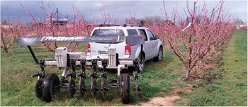
The research was conducted in a peach orchard (Prunus persica cv. ‘Platycarpa’) located at the IRTA Experimental Station (41°39’’19’N, 0°23’’36’E, ETRS89) in Gimenells (Lleida, Spain). The plot covered an area of 0.65 ha, and was planted in 2011 according to a 5×2.80 m pattern (Fig. 1). Soil was classified as Petrocalcic Calcixerept (Soil Survey Staff, 2014), and it was a well-drained soil without salinity problems. The presence of a petrocalcic horizon at a variable depth and high CaCO3 content were the main soil limiting factors. The climate is typical of semi-arid areas, with strong seasonal temperature variations (cold winters and hot summers) and an annual precipitation usually below 400 mm. Since 1946, the plot was cultivated with different crops and was modified at least four times in shape and size in order to adapt the parcelling of the farm.
Study plot and Veris 3100 soil sensor for ECa surveying.

Methodology
Sample size
Three production and quality variables were sampled within the plot: yield (kg/tree), fruit firmness (kg) and the refractometric index (°Baumé). To determine the sample size, an aerial multi-spectral image was taken on June 9th, 2015 and used as reference information. The image had a resolution of 0.25 m/pixel. Once the canopies were delimited (ESRI® ArcMapTM 10.0), a weighted average value of NDVI according to the area of the canopy was assigned to each tree. These individual values were then used as base data for determining the sample size through the application of the following formula:
 $$n\,{\equals}\,{{\zeta _{{\alpha /2}}^{2} {\times}CV^{2} } \over {E_{R}^{2} }}$$
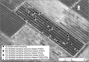
where n is the sample size, ζ α/2 (1.96) the value of the standard normal variate (SNV) for a 95% confidence (α=0.05), CV the Coefficient of Variation (in our case, 17.5%), and E R the relative error assumed (10%). The result was 12 sampling points that were randomly distributed within the plot (sampling scheme A). Additional schemes were tested in which new sampling points (twelve in each case) were first stratified according to two and three classes of NDVI (cluster analysis). NDVI classified maps were obtained by clustering the interpolated NDVI values (NDVI raster map). The same strategy (stratified sampling) was repeated using the information provided by a Veris 3100 soil sensor. This sensor measured the ECa at two soil depths: shallow (0–30 cm) and deep (0–90 cm). Both ECa values were interpolated, and ECa classes were established based on the cluster analysis of the two maps (shallow and deep) simultaneously. Finally, obtaining two and three classes (strata) was repeated by taking all three ancillary layers, NDVI, shallow ECa and deep ECa. In short, seven sampling schemes (including scheme A) were compared to each other based on a total number of 84 trees (7×12) within the plot (Fig. 2).
Sampling points corresponding to 7 different sampling schemes.

Sample stratification using ancillary data. Implications in estimation
In a SRS approach, the sample mean
 $$\left( {\bar{z}} \right)$$
has proven to be an unbiased estimator of the population mean (μ), with a variance that can be calculated by
 $\widehat{{ \sigma }}^{2} \left( {\bar{z}} \right)\,{\equals}\,s^{2}/n$
(s, standard deviation of the sample). As our interest is to work with small samples, confidence limits for the mean can be formulated as
 $\bar{z}\,\pm\,t_{{\alpha /2}} {\times}{s \over {\sqrt n }}$
, where
 $\bar{z}$
is the sample mean,
 $$s/\sqrt n $$
the standard error of the mean, and t
α/2 the Student’s t corresponding to n-1 degrees of freedom for a 95% confidence.
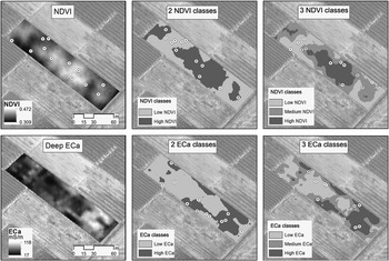
As mentioned above, in order to sample more evenly we used other sampling schemes by stratifying the 12 sampling points according to two strata (6 points/stratum) or three strata (4 points/stratum). The strata corresponded to the classes obtained after classification of the plot according to NDVI, ECa or both auxiliary data. Sampling points within each stratum were randomly distributed. Figure 3 shows five of the proposed sampling schemes, (i) SRS (scheme A), (ii) stratified sampling based on two classes of NDVI (scheme B1), (iii) stratified sampling based on three classes of NDVI (scheme B2), (iv) stratified sampling based on two classes of ECa (scheme C1), and (v) stratified sampling based on three classes of ECa (scheme C2). Schemas that use both layers of information (schemas D1 and D2) are not shown.
Sampling schemes: (i) simple random sampling (SRS), (ii) stratified sampling by NDVI (two strata), (iii) stratified sampling by NDVI (three strata), (iv) stratified sampling by ECa (two strata), (v) stratified sampling by ECa (three strata).

The different stratifications produced classes that were not equal in area, and so the mean (μ) was then estimated for K classes (strata) within the plot using a weighted average (Webster and Lark, Reference Webster and Lark2013):
 $$\bar{z}\,{\equals}\,\mathop{\sum}\nolimits_{k{\equals}1}^K {w_{k} } {\times}\bar{z}_{k} $$
where
 $\bar{z}_{k} $
was the average of the kth class, and w
k allowed the area of the kth class to be weighted:
 $${\rm }w_{k} \,{\equals}\,{{area\,of\,class\,k} \over {total\,plot\,area}}$$
As in SRS, confidence limits were obtained using the standard error of the mean, in this case, the square root of the estimated variance (Webster and Lark, Reference Webster and Lark2013):
 $$s^{2} \left( {\bar{z}} \right)\,{\equals}\,\mathop{\sum}\limits_{k{\equals}1}^K {{{w_{k}^{2} {\times}s_{k}^{2} } \over {n_{k} }}} $$
where
 $s_{k}^{2} $
was the within-class variance of the kth stratum, and n
k
the sampling points within the stratum (6 or 4).
Sampling efficiency
Taking the 84 sampling points as a representative distribution of values for the whole plot, each sampling scheme was compared to that distribution in terms of accuracy and efficiency. The efficiency to estimate the mean (μ) was established as the inverse of the estimated variance of the sample mean. The comparison of any of the sampling schemes (
 $\bar{z}$
) with respect to random sampling with 84 points (
 $\bar{z}_{{84}} $
) was carried out by calculating the relative efficiency (RE):
 $$RE\,\left( {\bar{z}/\bar{z}_{{84}} } \right)\,{\equals}\,{{Efficiency\,\left( {\bar{z}} \right)} \over {Efficiency\,\left( {\bar{z}_{{84}} } \right)}}\,{\equals}\,{{s^{2} \left( {\bar{z}_{{84}} } \right)} \over {s^{2} \left( {\bar{z}} \right)}}$$
The accuracy (%) of the mean estimation was assessed by the following expression:
 $${{\left| {\left( {\bar{z}{\minus}\bar{z}_{{84}} } \right)} \right|} \over {\bar{z}_{{84}} }}{\times}100$$
The proposed sampling schemes were based on a previous classification of the plot. A more accurate and efficient estimation of the mean was linked to the ability of the NDVI and/or ECa auxiliary layers to discriminate different average values between classes while the values within the classes were more or less homogeneous. A parameter that served to judge the goodness of these classifications was the relative variance (
 $r_{V} \,{\equals}\,s_{W}^{2} /s_{T}^{2} $
), where
 $s_{W}^{2} $
was the pooled or average within-class variance, and
 $s_{T}^{2} $
was the total variance in the sample (Webster and Lark, Reference Webster and Lark2013). Used in the form of its complement
 $$1\,{\minus}\,\left( {s_{W}^{2} \,/\,s_{T}^{2} } \right)\,{\equals}\,1\,{\minus}\,r_{V} $$
allowed values close to 1 to be obtained for those more effective sampling schemes. Values close to 0 or even negative corresponded to non-effective stratifications.
Results
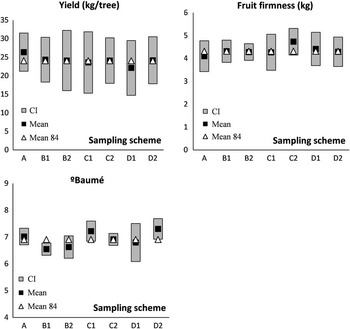
Figure 4 shows the comparison between the different sampling schemes tested. For each of the variables (yield, fruit firmness and °Baumé), confidence intervals (CI) for the population mean (μ) were obtained. In the same figure, the mean of each sample was compared to the average calculated for the 84 sampling points within the plot (mean 84). The proximity between these two values was taken as a measure of accuracy, while the amplitude of the CIs could be interpreted in terms of sampling efficiency (greater precision or efficiency was associated with narrower intervals around the sample mean).
Comparison between sampling schemes: A (SRS); B1 and B2 (NDVI stratified sampling, 2 and 3 classes, respectively); C1 and C2 (ECa stratified sampling, 2 and 3 classes, respectively); D1 and D2 (combined NDVI+ECa stratified sampling, 2 and 3 classes, respectively).

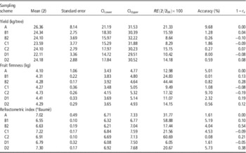
The main results include (i) stratified sampling improved accuracy compared to SRS; (ii) stratified sampling was not always more efficient than SRS; and (iii) there was a greater disparity between methods in estimating fruit quality (°Baumé). Table 1 shows the efficiency results of each sampling scheme.
Accuracy and efficiency parameters for the sampling schemes tested

A (Simple random sampling); B1 and B2 (NDVI stratified sampling, 2 and 3 classes); C1 and C2 (ECa stratified sampling, 2 and 3 classes); D1 and D2 (combined NDVI+ECa stratified sampling, 2 and 3 classes). RE (Relative Efficiency). r v (relative variance).
Discussion
Sampling to estimate yield
Compared to the other sampling schemes, SRS (scheme A) obtained the greatest inaccuracy in estimating the yield (almost 10%). However, this value could be considered as acceptable given the criterion adopted by other researchers (Carrillo et al., Reference Carrillo, Matese, Rousseau and Tisseyre2016). When stratifying the samples using the NDVI or the ECa, the sample means worked even better achieving very good accuracy values below 2% (Table 1). This was expected because of the possible spatial covariation between the NDVI (indicative of tree vigor) and yield, or between ECa (indicative of soil characteristics) and yield, as Martínez-Casasnovas et al. (Reference Martínez-Casasnovas, Agelet-Fernandez, Arno and Ramos2012) and Corwin and Lesch (Reference Corwin and Lesch2005) respectively refer. Although stratified sampling performed better in terms of accuracy, the expectation of a clear superiority of the method was not met when the efficacy of the classification is judged. In all cases, stratifications were shown to be ineffective (very low 1–r v values). This result was more or less equivalent to the efficiencies obtained (RE) for the different sampling schemes. In this regard, no stratification was more efficient than SRS, although the latter was less accurate (Table 1).
Considering both the accuracy and the efficiency, our recommendation for the best yield estimation is to use the ECa map to stratify the sample into three classes (scheme C2). Using the NDVI (2 classes) is another possibility (scheme B1). However, the significant relationship between yield and ECa values (higher ECa within the plot was associated with lower yields) made it advisable to stratify on the basis of this information layer (data not shown). The influence of CaCO3 (with high presence in the soil and spatial variation) on the ECa signal and yield could explain this convenience.
Sampling to estimate quality parameters
Sampling schemes worked differently when estimating quality parameters. Regarding fruit firmness (Table 1), scheme B2 was clearly better in both accuracy (<1%) and efficiency (RE above the other sampling schemes). A significant correlation between NDVI and firmness (the greater the NDVI, the greater the firmness) could explain this result. Likewise, stratifying sampling points based on the NDVI allowed spatial classification in fruit firmness to be more effective (1–r v =0.28). SRS in refractometric index estimation (°Baumé) was very accurate and efficient, and was only surpassed by the C2 sampling scheme. However, NDVI correlated inversely and significantly with this quality parameter (not the ECa), and sampling points were optimally classified using three classes of NDVI. B2 sampling could again be the scheme to use given its accuracy (4%) and acceptable efficiency (Table 1).
Conclusion
The use of ancillary data such as NDVI or ECa allows improving yield and quality estimates by stratifying samples within the orchards in comparison to simple random sampling (SRS). However, yield estimation may require a different information layer (ECa) than that used to stratify sampling to estimate quality parameters (NDVI). In any case, sampling schemes that stratify into three classes perform better in both accuracy and efficiency than sampling based on two classes or strata. The combined use of NDVI and ECa does not provide substantial advantages compared to the use of a single layer of information, especially when both layers are unrelated.
Acknowledgements
The authors thank the IRTA Experimental Station in Gimenells (Lleida, Spain) for the possibility of carrying out a sampling study on a peach orchard.