1 Introduction
Electron–positron plasmas can exist in accretion disks (Orosz et al. Reference Orosz, Remillard, Bailyn and McClintock1997), active galactic nuclei (Michel Reference Michel1982), black holes (Daniel & Tajima Reference Daniel and Tajima1998) and pulsar magnetospheres (Max & Perkins Reference Max and Perkins1972). Electron–positron plasmas can also exist in laboratory plasmas in which the positrons are used to probe the particle transportation and the propagation of an intense laser pulse in plasmas (Berezhiani, Tsintsadze & Shukla Reference Berezhiani, Tsintsadze and Shukla1992). Since a majority of the astrophysical plasmas contain ions in addition to the electrons and positrons, it is of significance to investigate the linear or nonlinear waves in electron–positron–ion (EPI) plasmas. The nonlinear collective excitation in EPI plasmas has been discovered by many authors. The presence of the positrons in EPI plasmas can result in a reduction of the ion-acoustic soliton amplitude (Popel, Vladimirov & Shukla Reference Popel, Vladimirov and Shukla1995). Recently both small- and arbitrary-amplitude solitary waves (El-Awady et al. Reference El-Awady, El-Tantawy, Moslem and Shukla2010), dressed solitons (Tiwari Reference Tiwari2008), Alfvén waves (Kakati & Goswami Reference Kakati and Goswami1998), drift waves (Saleem, Haque & Vranješ Reference Saleem, Haque and Vranješ2003) and head-on collisions of ion-acoustic solitary waves (Chatterjee et al. Reference Chatterjee, Ghosh, Roy, Muniandy, Wong and Sahu2010) have been well studied in EPI plasmas, where the wave modes in EPI plasmas behaved very differently in the relativistic regime (Saeed & Shah Reference Saeed and Shah2010).
When a plasma is cooled to a relatively low temperature or its number density is relatively high, the thermal de Broglie wavelength of the charged particles becomes comparable to the dimension of the distance between the charged particles. Accordingly, quantum effects should be considered in dense plasmas (Chandra & Ghosh Reference Chandra and Ghosh2012; Sahu & Ghosh Reference Sahu and Ghosh2013; Wang, Lü & Eliasson Reference Wang, Lü and Eliasson2013a ; Wang, Shukla & Eliasson Reference Wang, Shukla and Eliasson2013b ; El-Labany et al. Reference El-Labany, El-Taibany, El-Samahy, Hafez and Atteya2014; Irfan, Ali & Mirza Reference Irfan, Ali and Mirza2014; Saha & Chatterjee Reference Saha and Chatterjee2014; Wang & Eliasson Reference Wang and Eliasson2014). Quantum effects, together with those of the ion kinematic viscosity (Roy, Misra & Chatterjee Reference Roy, Misra and Chatterjee2008; Han et al. Reference Han, He, Yang, Han and Wang2011) and non-planar (Sabry, Moslem & Shukla Reference Sabry, Moslem and Shukla2009) or weakly nonlinear or arbitrarily nonlinear (Ali et al. Reference Ali, Moslem, Shukla and Schlickeiser2007) quantum ion-acoustic waves have been intensively studied in quantum EPI plasmas. Under some extreme conditions, relativistic degenerate effects of electrons and positrons were also considered to study nonlinear excitation in quantum EPI plasmas (Sabry, Moslem & Shukla Reference Sabry, Moslem and Shukla2012) or dusty quantum EPI plasmas (Roy, Tasnim & Mamun Reference Roy, Tasnim and Mamun2012).
In fact quantum magnetosonic waves have also been investigated recently by many authors in high-density and low-temperature magnetized quantum plasmas (Misra & Shukla Reference Misra and Shukla2008; Mushtaq & Qamar Reference Mushtaq and Qamar2009; Mushtaq & Vladimirov Reference Mushtaq and Vladimirov2010, Reference Mushtaq and Vladimirov2011; Akbari-Moghanjoughi Reference Akbari-Moghanjoughi2011; Mushtaq et al.
Reference Mushtaq, Maroof, Ahmad and Qamar2012; Wang et al.
Reference Wang, Zhou, Qiu, Wang and Lu2012; Maroof, Mushtaq & Qamar Reference Maroof, Mushtaq and Qamar2016). The collective modes in magnetized quantum plasmas can be studied using quantum magnetohydrodynamic theory, which includes a quantum correction term called the Bohm potential. Both slow and fast magnetosonic waves have been investigated in quantum plasmas including the spin effects (Marklund & Brodin Reference Marklund and Brodin2007) via the spin force and macroscopic spin magnetization current (Mushtaq & Vladimirov Reference Mushtaq and Vladimirov2010). The presence of spin-
 $1/2$
effects can modify the shape of the magnetosonic solitary waves (Marklund, Eliasson & Shukla Reference Marklund, Eliasson and Shukla2007) and decrease the modulational instability growth rate as the normalized Zeeman energy does not exceed a critical value (Misra & Shukla Reference Misra and Shukla2008). The propagation of quantum magnetosonic waves was studied by using the relativistic magnetic susceptibility in a Fermi–Dirac plasma in the presence of the spin magnetization effect (Akbari-Moghanjoughi Reference Akbari-Moghanjoughi2011).
On the other hand, the linear and nonlinear waves in strongly coupled plasmas are quite different from those in weakly coupled systems (Ikezi Reference Ikezi1986). The strong coupling of the ions can significantly modify the dispersion properties of collective plasma modes as well as the characteristics of nonlinear structures such solitons and shocks. The ions can enter the strongly coupled regime when the Coulomb coupling parameter
 ${\it\Gamma}=(Z_{i}e)^{2}/(4{\rm\pi}{\it\varepsilon}_{0}a_{i}k_{B}T_{i})$
is larger than unity, where
 $a_{i}=(3/4{\rm\pi}n_{i0})^{1/3}$
is the Wigner–Seitz radius of the ions,
 $e$
is the elementary charge and
 $Z_{i}$
,
 $T_{i}$
and
 $n_{i0}$
are the charge number, temperature and number density of ions, respectively. The dynamic characteristic of the strongly coupled ions can be described by a generalized hydrodynamic (GH) model. This phenomenological model has been validated over a wide range of the coupling parameter
 ${\it\Gamma}$
, from the weakly coupled case
 $({\it\Gamma}\ll 1)$
to the strongly coupled case
 $(1\ll {\it\Gamma}<{\it\Gamma}_{c})$
. For the GH model, there are two different regimes: the ‘hydrodynamic regime’
 $({\it\omega}{\it\tau}_{m}\ll 1)$
and the ‘kinetic regime’
 $({\it\omega}{\it\tau}_{m}\gg 1)$
, where
 ${\it\omega}^{-1}$
is the typical time scale of the wave and
 ${\it\tau}_{m}$
is the memory (viscoelastic) relaxation time. In the hydrodynamic regime, one can obtain the normal hydrodynamic equation which describes longitudinal acoustic waves suffering viscous dissipation (Veeresha et al.
Reference Veeresha, Tiwari, Sen, Kaw and Das2010). While in the kinetic limit, not only longitudinal acoustic waves (Ghosh et al.
Reference Ghosh, Gupta, Chakrabarti and Chaudhuri2011) but also transverse shear waves are considered to be formed (Kaw & Sen Reference Kaw and Sen1998) as the viscoelastic relaxation is not instantaneous.
Recently, the properties of solitary and shock structures were also presented in a dense plasma composed of strongly coupled non-degenerate ions and degenerate electrons (Shukla, Mamun & Mendis Reference Shukla, Mamun and Mendis2011). It was noted that the amplitude, speed and width of the solitary and shock waves depended sensitively on the electron degenerate effects and the strong coupling between ions (Ghosh, Chakrabarti & Shukla Reference Ghosh, Chakrabarti and Shukla2012). The modulational instability and evolution of wave packets in both the weakly relativistic limit and the ultrarelativistic limit was considered in strongly coupled quantum plasmas (Misra & Shukla Reference Misra and Shukla2012), which shows that the solitary wave packets with short wavelengths were stable in the weakly relativistic limit, whereas they could be very different in the ultrarelativistic limit.
The investigation of magnetosonic waves in strongly coupled quantum EPI plasmas has important potential applications in space and fusion plasmas, where they are utilized in particle acceleration and heating experiments. Motivated by the works mentioned above, we will investigate nonlinear two-dimensional magnetosonic solitary and shock waves in dense magnetized plasmas, which consist of strongly coupled ions and quantum electrons and positrons. We account for strong coupling between the ions by using a generalized viscoelastic hydrodynamic model (Gozadinos, Ivlev & Boeuf Reference Gozadinos, Ivlev and Boeuf2003) along with the pressure as prescribed by Yaroshenko et al. (Reference Yaroshenko, Verheest, Thomas and Morfill2009). We use a quantum hydrodynamics (QHD) model with the effects of quantum diffraction as well as quantum statistic effects for both electrons and positrons. Both the hydrodynamic and kinetic regimes will be investigated in this paper.
2 Plasmas model
2.1 Basic equations
We consider the nonlinear propagation of magnetosonic waves in a magnetized plasma consisting of strongly coupled classical ions and weakly coupled degenerate electrons and positrons. The applied magnetic field is along the
 $z$
-axis
 $\boldsymbol{B}_{0}=B_{0}\hat{\boldsymbol{e}}_{z}$
, where
 $\hat{\boldsymbol{e}}_{z}$
is the unit vector of the
 $z$
-axis and
 $B_{0}$
is the strength of the applied magnetic field. As we consider a magnetosonic wave with a weakly transverse perturbation, it is not a complete two-dimensional wave but a one-dimensional wave with a transverse perturbation. For relatively massive ions, the collision rate of ions with electrons and positrons is negligible. We ignore the quantum statistical and diffraction effects due to the relatively large inertia of ions. Here, strong coupling is defined in terms of the usual Coulomb coupling parameter. In the crust of neutron stars and in the cores of white dwarfs, the strongly correlated ions are embedded into a degenerate Fermi gas of electrons or positrons, where the Fermi electron or positron temperature
 $T_{Fe(Fp)}$
is much higher than the plasma electron temperature
 $T_{e(p)}$
. Thus, such dense astrophysical plasmas can be regarded as strongly correlated quantum plasmas (Ichimaru, Iyetomi & Tanaka Reference Ichimaru, Iyetomi and Tanaka1987; Akbari-Moghanjoughi & Ghorbanalilu Reference Akbari-Moghanjoughi and Ghorbanalilu2015). Accordingly, the dynamics of strongly coupled ions can be described by the continuity equation and GH model, which reads (Kaw & Sen Reference Kaw and Sen1998)
 $$\begin{eqnarray}\displaystyle & \displaystyle \frac{\partial n_{i}}{\partial t}+\boldsymbol{{\rm\nabla}}\boldsymbol{\cdot }(n_{i}\boldsymbol{v}_{i})=0, & \displaystyle\end{eqnarray}$$
 $$\begin{eqnarray}\displaystyle & \displaystyle \left(1+{\it\tau}_{m}\frac{\text{d}}{\text{d}t}\right)\left[m_{i}n_{i}\frac{\text{d}\boldsymbol{v}_{i}}{\text{d}t}-Z_{i}en_{i}(\boldsymbol{E}+\boldsymbol{v}_{i}\times \boldsymbol{B})+\boldsymbol{{\rm\nabla}}P_{i}\right]={\it\eta}{\rm\nabla}^{2}\boldsymbol{v}_{i}+\left({\it\xi}+\frac{{\it\eta}}{3}\right)\boldsymbol{{\rm\nabla}}(\boldsymbol{{\rm\nabla}}\boldsymbol{\cdot }\boldsymbol{v}_{i}). & \displaystyle \nonumber\\ \displaystyle & & \displaystyle\end{eqnarray}$$
 $$\begin{eqnarray}\displaystyle & \displaystyle \frac{\partial n_{e}}{\partial t}+\boldsymbol{{\rm\nabla}}\boldsymbol{\cdot }(n_{e}\boldsymbol{v}_{e})=0, & \displaystyle\end{eqnarray}$$
 $$\begin{eqnarray}\displaystyle & \displaystyle m_{e}n_{e}\frac{\text{d}\boldsymbol{v}_{e}}{\text{d}t}=-en_{e}(\boldsymbol{E}+\boldsymbol{v}_{e}\times \boldsymbol{B})-\boldsymbol{{\rm\nabla}}P_{e}+\frac{\hbar ^{2}}{2m_{e}}n_{e}\boldsymbol{{\rm\nabla}}\left(\frac{{\rm\nabla}^{2}\sqrt{n_{e}}}{\sqrt{n_{e}}}\right). & \displaystyle\end{eqnarray}$$
 $$\begin{eqnarray}\displaystyle & \displaystyle \frac{\partial n_{p}}{\partial t}+\boldsymbol{{\rm\nabla}}\boldsymbol{\cdot }(n_{p}\boldsymbol{v}_{p})=0, & \displaystyle\end{eqnarray}$$
 $$\begin{eqnarray}\displaystyle & \displaystyle m_{p}n_{p}\frac{\text{d}\boldsymbol{v}_{p}}{\text{d}t}=en_{p}(\boldsymbol{E}+\boldsymbol{v}_{p}\times \boldsymbol{B})-\boldsymbol{{\rm\nabla}}P_{p}+\frac{\hbar ^{2}}{2m_{p}}n_{p}\boldsymbol{{\rm\nabla}}\left(\frac{{\rm\nabla}^{2}\sqrt{n_{p}}}{\sqrt{n_{p}}}\right). & \displaystyle\end{eqnarray}$$
 $$\begin{eqnarray}\displaystyle & \displaystyle \boldsymbol{{\rm\nabla}}\times \boldsymbol{B}={\it\mu}_{0}\boldsymbol{J}+\frac{1}{c^{2}}\frac{\partial \boldsymbol{E}}{\partial t}, & \displaystyle\end{eqnarray}$$
 $$\begin{eqnarray}\displaystyle & \displaystyle \boldsymbol{{\rm\nabla}}\times \boldsymbol{E}=-\frac{\partial \boldsymbol{B}}{\partial t}. & \displaystyle\end{eqnarray}$$
 $n_{j}$
,
 $\boldsymbol{v}_{j}$
and
 $m_{j}$
respectively denote the number density (with equilibrium value
 $n_{j0}$
), velocity and mass of different species (
 $j=i$
for ions,
 $j=e$
for electrons and
 $j=p$
for positrons).
 $Z_{i}$
is the ion charge number,
 $e$
is the elementary charge and
 $\hbar$
is the Planck constant divided by
 $2{\rm\pi}$
. In (2.7) and (2.8),
 $\boldsymbol{J}$
is the current density and
 $\boldsymbol{E}$
and
 $\boldsymbol{B}$
(with equilibrium value
 $\boldsymbol{B}_{0}$
) are the electric field and magnetic field, respectively. Furthermore,
 $P_{j}$
is the classical pressure for ions and quantum statistical pressure for electrons and positrons, and
 $\text{d}/\text{d}t=\partial /\partial t+\boldsymbol{v}_{j}\boldsymbol{\cdot }\boldsymbol{{\rm\nabla}}$
is the convective derivative. In equilibrium one has
 $Z_{i}n_{i0}+n_{p0}=n_{e0}$
. In (2.2),
 ${\it\tau}_{m}$
denotes the viscoelastic relaxation time as (Kaw & Sen Reference Kaw and Sen1998)
 $$\begin{eqnarray}{\it\tau}_{m}=\frac{{\it\xi}+4{\it\eta}/3}{n_{i0}k_{B}T_{i}}\left[1-{\it\gamma}_{i}{\it\mu}_{i}+\frac{4}{15}u({\it\Gamma}_{i})\right]^{-1},\end{eqnarray}$$
where
 $T_{i}$
is the ion temperature,
 $k_{B}$
is the Boltzmann constant and
 ${\it\xi}+4{\it\eta}/3$
is the coefficient of the effective ion viscosity in which
 ${\it\xi}$
and
 ${\it\eta}$
represent the bulk and the shear viscosity, respectively.
 ${\it\gamma}_{i}=5/3$
is the ion adiabatic index. The compressibility
 ${\it\mu}_{i}$
is given by (Kaw & Sen Reference Kaw and Sen1998)
 $$\begin{eqnarray}{\it\mu}_{i}=\frac{1}{k_{B}T_{i}}\left(\frac{\partial P_{i}}{\partial n_{i}}\right)_{T_{i}}=1+\frac{1}{3}u({\it\Gamma}_{i})+\frac{{\it\Gamma}_{i}}{9}\frac{\partial u({\it\Gamma}_{i})}{\partial {\it\Gamma}_{i}},\end{eqnarray}$$
where
 $u({\it\Gamma}_{i})$
is a measure of the excess internal ion energy. Here
 ${\it\Gamma}_{i}$
is the ion coupling parameter which will be presented in detail later. The expression for
 $u({\it\Gamma}_{i})$
can be obtained for
 ${\it\kappa}\rightarrow 0$
as (Slattery, Doolen & DeWitt Reference Slattery, Doolen and DeWitt1980)
 $$\begin{eqnarray}u({\it\Gamma}_{i})\approx \left\{\begin{array}{@{}ll@{}}\displaystyle -0.90{\it\Gamma}_{i}+0.95{\it\Gamma}_{i}^{1/4}+0.18{\it\Gamma}_{i}^{-1/4}-0.80, & (1\leqslant {\it\Gamma}_{i}\leqslant 160)\\ \displaystyle 1.5-0.90{\it\Gamma}_{i}+2980{\it\Gamma}_{i}^{-2}, & (160<{\it\Gamma}_{i}\leqslant 300)\\ \displaystyle 1.5-0.90{\it\Gamma}_{i}+9.6{\it\Gamma}_{i}^{-1}+840{\it\Gamma}_{i}^{-2}+1.1\times 10^{5}{\it\Gamma}_{i}^{-3} & (300<{\it\Gamma}_{i}\leqslant 2000).\end{array}\right.\end{eqnarray}$$
We note that the relaxation time
 ${\it\tau}_{m}$
represents two characteristic time scales to depict two classes of wave modes, namely, the kinetic modes with
 ${\it\omega}{\it\tau}_{m}\gg 1$
and the hydrodynamic modes with
 ${\it\omega}{\it\tau}_{m}\ll 1$
.
Here we consider degenerate electrons and positrons. The degenerate parameter
 ${\it\chi}_{j}=\hbar ^{2}(3{\rm\pi}^{2})^{2/3}n_{i0}^{2/3}/2m_{j}k_{B}T_{i}$
for particles of species
 $j$
should be larger than one. One should consider that the number density
 $n_{j0}$
exceeds the quantum concentration
 $n_{qj}=(2m_{j}k_{B}T_{i}/\hbar ^{2})^{3/2}/3{\rm\pi}^{2}$
. For degenerate electrons and positrons, the energy distribution is no longer a thermal distribution but a Fermi distribution. The equation of pressure for non-relativistic degenerate electrons (positrons) is given by (Shukla & Eliasson Reference Shukla and Eliasson2011)
 $$\begin{eqnarray}P_{e(p)}=\frac{1}{10}\frac{\hbar ^{2}}{m_{e(p)}}\left(3{\rm\pi}^{2}\right)^{2/3}n_{e(p)}^{5/3}=\frac{k_{B}T_{Fe(p)}}{5n_{e0(p0)}^{2/3}}n_{e}^{5/3}.\end{eqnarray}$$
The core of a white dwarf has a high average bulk density where the electrons are relativistically degenerate. In the outer mantle, with lower density, the electrons may be weakly relativistic degenerate. Nonlinear solitary waves and shock waves were studied in relativistic degenerate electron and positron plasmas in Ali & ur Rahman (Reference Ali and ur Rahman2014). The last terms of (2.4) and (2.6) are called the Bohm potential and represent for quantum diffraction effects (Haas Reference Haas2005). We consider the ion pressure in (2.2) as (Shukla et al. Reference Shukla, Mamun and Mendis2011)
 $$\begin{eqnarray}\boldsymbol{{\rm\nabla}}P_{i}={\it\gamma}_{i}k_{B}T_{if}\boldsymbol{{\rm\nabla}}n_{i},\end{eqnarray}$$
where
 $T_{if}=T_{\ast }+{\it\mu}_{i}T_{i}$
is the effective temperature in which
 $T_{\ast }$
, coming from the electrostatic interactions between the strongly coupled ions, is given by (Yaroshenko et al.
Reference Yaroshenko, Verheest, Thomas and Morfill2009)
 $$\begin{eqnarray}T_{\ast }=\frac{N_{nn}}{3}{\it\Gamma}_{i}T_{i}(1+{\it\kappa})\text{e}^{-{\it\kappa}},\end{eqnarray}$$
where
 $N_{nn}$
is the number of nearest neighbours (e.g.
 $N_{nn}=12$
for the face centered cubic lattices and
 $N_{nn}=8$
for the body centered cubic lattice). Also
 ${\it\kappa}=a_{i}/{\it\lambda}_{Di}$
, where
 ${\it\lambda}_{Di}=\sqrt{{\it\varepsilon}_{0}T_{i}/n_{i0}Z_{i}^{2}\text{e}^{2}}$
is the ion Debye length. For increasing values of
 ${\it\Gamma}_{i}$
,
 $T_{\ast }$
may be comparable or even dominate over
 ${\it\mu}_{i}T_{i}$
for
 ${\it\Gamma}_{i}\gg 1$
.
It is convenient to rewrite the basic equations (2.1)–(2.8) in normalized form as
 $$\begin{eqnarray}\displaystyle & \displaystyle \frac{\partial n_{j}}{\partial t}+\boldsymbol{{\rm\nabla}}\boldsymbol{\cdot }(n_{j}\boldsymbol{v}_{j})=0, & \displaystyle\end{eqnarray}$$
 $$\begin{eqnarray}\displaystyle & \displaystyle \left(1+{\it\tau}_{m}\frac{\text{d}}{\text{d}t}\right)\left[n_{i}\frac{\text{d}\boldsymbol{v}_{i}}{\text{d}t}-Z_{i}n_{i}(\boldsymbol{E}+\boldsymbol{v}_{i}\times \boldsymbol{B})+{\it\beta}\boldsymbol{{\rm\nabla}}n_{i}\right]={\it\eta}{\rm\nabla}^{2}\boldsymbol{v}_{i}+\left({\it\xi}+\frac{{\it\eta}}{3}\right)\boldsymbol{{\rm\nabla}}(\boldsymbol{{\rm\nabla}}\boldsymbol{\cdot }\boldsymbol{v}_{i}), & \displaystyle \nonumber\\ \displaystyle & & \displaystyle\end{eqnarray}$$
 $$\begin{eqnarray}\displaystyle & \displaystyle \frac{\text{d}\boldsymbol{v}_{e}}{\text{d}t}=-M\left(\boldsymbol{E}+\boldsymbol{v}_{e}\times \boldsymbol{B}+\frac{{\it\beta}_{1}}{3}n_{e}^{-1/3}\boldsymbol{{\rm\nabla}}n_{e}\right)+\frac{H^{2}}{2}\boldsymbol{{\rm\nabla}}\left(\frac{{\rm\nabla}^{2}\sqrt{n_{e}}}{\sqrt{n_{e}}}\right), & \displaystyle\end{eqnarray}$$
 $$\begin{eqnarray}\displaystyle & \displaystyle \frac{\text{d}\boldsymbol{v}_{p}}{\text{d}t}=-M\left(\boldsymbol{E}+\boldsymbol{v}_{p}\times \boldsymbol{B}+\frac{{\it\beta}_{2}}{3}n_{p}^{-1/3}\boldsymbol{{\rm\nabla}}n_{p}\right)+\frac{H^{2}}{2}\boldsymbol{{\rm\nabla}}\left(\frac{{\rm\nabla}^{2}\sqrt{n_{p}}}{\sqrt{n_{p}}}\right), & \displaystyle\end{eqnarray}$$
 $$\begin{eqnarray}\displaystyle & \displaystyle \boldsymbol{{\rm\nabla}}\times \boldsymbol{B}=Z_{i}(n_{i}\boldsymbol{v}_{i}+{\it\mu}n_{p}\boldsymbol{v}_{p}-{\it\nu}n_{e}\boldsymbol{v}_{e})+{\it\gamma}\frac{\partial \boldsymbol{E}}{\partial t}, & \displaystyle\end{eqnarray}$$
 $$\begin{eqnarray}\displaystyle & \displaystyle \boldsymbol{{\rm\nabla}}\times \boldsymbol{E}=-\frac{\partial \boldsymbol{B}}{\partial t}. & \displaystyle\end{eqnarray}$$
 $n_{j}^{\prime }=n_{j}/n_{j0}$
,
 $\boldsymbol{v}_{j}^{\prime }=\boldsymbol{v}_{j}/v_{A}$
,
 $t^{\prime }={\it\Omega}_{i}t$
, where
 $j=i$
for ions,
 $j=e$
for electrons and
 $j=p$
for positrons. The space is normalized by
 $v_{A}/{\it\Omega}_{i}$
.
 ${\it\Omega}_{i}=eB_{0}/m_{i}$
is the ion cyclotron frequency and
 $v_{A}=B_{0}/\sqrt{{\it\mu}_{0}n_{i0}m_{i}}$
is the Alfvén speed. We also have
 ${\it\tau}_{m}^{\prime }={\it\Omega}_{i}{\it\tau}_{m}$
,
 ${\it\eta}^{\prime }={\it\eta}{\it\Omega}_{i}/(m_{i}n_{i0}v_{A}^{2})$
,
 ${\it\xi}^{\prime }={\it\xi}{\it\Omega}_{i}/(m_{i}n_{i0}v_{A}^{2})$
,
 $\boldsymbol{E}^{\prime }=e\boldsymbol{E}/(m_{i}{\it\Omega}_{i}v_{A})$
,
 $\boldsymbol{B}^{\prime }=\boldsymbol{B}/B_{0}$
. And the dimensionless parameters adopted in (2.15)–(2.20) are
 ${\it\beta}={\it\gamma}_{i}k_{B}T_{if}/m_{i}v_{A}^{2}$
,
 $M=m_{i}/m,m=m_{e}=m_{p},H=\hbar {\it\Omega}_{i}/mv_{A}^{2},{\it\beta}_{1}=C_{s1}^{2}/v_{A}^{2},{\it\beta}_{2}=C_{s2}^{2}/v_{A}^{2},C_{s1}=\sqrt{k_{B}T_{Fe}/m_{i}},C_{s2}=\sqrt{k_{B}T_{Fp}/m_{i}},{\it\gamma}=v_{A}^{2}/c^{2},{\it\mu}=n_{p0}/Z_{i}n_{i0}$
and
 ${\it\nu}=n_{e0}/Z_{i}n_{i0}$
. Now the overall charge-neutral condition can be overwritten as
 $1+{\it\mu}={\it\nu}$
. It is necessary to note that in (2.15)–(2.20) we neglect the superscript of the new variables for simplicity.
2.2 Parameter regimes
The quantum coupling parameter of degenerate particles is defined as
 ${\it\Gamma}_{qj}=q_{j}^{2}/(4{\rm\pi}{\it\varepsilon}_{0}a_{j}k_{B}T_{Fj})$
and the classical coupling parameter of non-degenerate particles is given by
 ${\it\Gamma}_{j}=q_{j}^{2}/(4{\rm\pi}{\it\varepsilon}_{0}a_{j}k_{B}T_{j})$
, where
 $q_{j}$
is the charge of
 $j$
species,
 $a_{j}=(3/4{\rm\pi}n_{j0})$
is the Wigner–Seitz radius,
 $T_{Fj}$
is the Fermi temperature and
 $T_{j}$
is the temperature. On the other hand, the degeneracy parameter for a particle of species
 $j$
is given by
 ${\it\chi}_{j}\equiv T_{Fj}/T_{j}=(1/2)(3{\rm\pi}^{2})^{2/3}(n_{j0}{\it\lambda}_{Bj}^{3})^{2/3}$
, where
 ${\it\lambda}_{Bj}=\hbar /\sqrt{k_{B}T_{j}m_{j}}$
is the thermal de Broglie wavelength. The particles are said to be non-degenerate if
 ${\it\chi}_{j}<1$
. Accordingly, quantum effects should be considered for the electrons and positrons while the ions should be considered as classical components due to their large mass. For strongly correlated the ions, the classical strong coupling parameter should be used while for electrons and positrons the quantum coupling parameter should be used. Thus the electron (positron) correlations are neglected as the electron–electron (positron–positron) correlation effects are negligibly small compared to ion–ion correlation effects, which can be easily seen from the relationship
 $$\begin{eqnarray}{\it\Gamma}_{e(p)}=\frac{\text{e}^{2}}{4{\rm\pi}{\it\varepsilon}_{0}a_{e(p)}k_{B}T_{Fe(Fp)}}=\frac{a_{i}}{a_{e(p)}}\frac{T_{i}}{T_{e(p)}}\frac{1}{Z^{2}}\frac{1}{{\it\chi}_{e(p)}}{\it\Gamma}_{i}\ll {\it\Gamma}_{i},\end{eqnarray}$$
as
 ${\it\chi}_{e(p)}\gg 1$
,
 $Z\geqslant 1$
,
 $T_{i}/T_{e(p)}<1$
and the Wigner–Seitz radius
 $a_{e(p)}$
is slightly smaller than
 $a_{i}$
.
Since in our model electrons and positrons are treated as quantum degenerate with weak interactions and the ions are treated as classical with strong coupling, we must have
 ${\it\chi}_{i}<1$
,
 ${\it\chi}_{e(p)}>1$
,
 ${\it\Gamma}_{qe(p)}<1$
and
 ${\it\Gamma}_{i}>1$
. It has been discovered that the viscosity coefficient
 ${\it\sigma}_{vis}\equiv ({\it\xi}+4{\it\eta}/3){\it\Omega}_{i}/(n_{i0}k_{B}T_{i})$
(
 ${\it\tau}_{m}$
being normalized by
 ${\it\Omega}_{i}^{-1}$
) in (2.9) has a wide minima (
 ${\sim}$
1) in
 $1<{\it\Gamma}_{i}<10$
and tends to grow as
 $\propto {\it\Gamma}_{i}^{4/3}$
for
 ${\it\Gamma}_{i}\geqslant 10$
(Kaw & Sen Reference Kaw and Sen1998). Furthermore, viscosity coefficient
 ${\it\sigma}_{vis}$
becomes high for
 ${\it\Gamma}_{i}<1$
. Hence
 ${\it\tau}_{m}(\propto {\it\sigma}_{vis})$
is high not only in the weak coupling regime, but also in the high coupling regime (
 ${\it\Gamma}_{i}\gg 1$
). So the kinetic modes requiring
 ${\it\omega}{\it\tau}_{m}\gg 1$
exist either in the weak coupling regime or in the strong coupling regime. On the other hand, in the range of
 $1<{\it\Gamma}_{i}<10$
,
 ${\it\tau}_{m}$
is typically of the order of unity, which shows that the kinetic condition may no longer be satisfied. Then we reach the hydrodynamic regime with
 ${\it\omega}{\it\tau}_{m}\ll 1$
. Thus we can specify two separate parameter regimes for the kinetic and hydrodynamic modes in the following.
Case I (Kinetic regime):
 ${\it\chi}_{i}<1,{\it\chi}_{e(p)}>1,{\it\Gamma}_{i}\gg 1,{\it\Gamma}_{e(p)}<1$
and
 ${\it\omega}{\it\tau}_{m}\gg 1$
. This represents the propagation of kinetic wave modes. In this case, the reasonable choice of parameters are
 $n_{e0}\sim 5\times 10^{36}~\text{m}^{-3},n_{i0}\sim 10^{35}~\text{m}^{-3},T_{i}\sim 5\times 10^{6}~\text{K},T_{e}\sim 10^{8}~\text{K}$
.
Case II (Hydrodynamic regime):
 ${\it\chi}_{i}<1,{\it\chi}_{e(p)}>1,1\leqslant {\it\Gamma}_{i}\geqslant 10,{\it\Gamma}_{e(p)}<1$
and
 ${\it\omega}{\it\tau}_{m}\ll 1$
. This represents the hydrodynamic wave modes existing in plasmas composed of weakly coupled degenerate quantum electrons and positrons and strongly coupled classical ions. The parameters in this regime are
 $n_{e0}\sim 5\times 10^{32}~\text{m}^{-3},n_{i0}\sim 5\times 10^{31}~\text{m}^{-3},T_{i}\sim 5\times 10^{5}~\text{K},T_{e}\sim 10^{6}~\text{K}$
.
In (2.17) and (2.18), the parameters
 ${\it\beta}_{1}$
and
 ${\it\beta}_{2}$
stand for the electron and positron Fermi temperature. In the next section, we will use the relationship
 ${\it\beta}_{2}=(1-1/{\it\nu})^{2/3}{\it\beta}_{1}$
, which comes from quasi-neutral equilibrium condition. Here we choose the above parameters in astrophysical dense plasma environments which are compatible with our model. We note that electron–positron annihilation can also be neglected safely for the above parameters (Ali et al.
Reference Ali, Moslem, Shukla and Schlickeiser2007).
3 Nonlinear evolution of magnetosonic waves
The normalized (2.15)–(2.20) generally have three magnetohydrodynamic modes, which are the slow magnetosonic waves, fast magnetosonic waves and Alfvén waves in the low-frequency limit. Here, we are interested in fast mode propagating perpendicular to external magnetic field. Here, we mainly consider the weak two-dimensional nonlinear magnetosonic waves with a transverse perturbation. The stretched coordinates are introduced as
 ${\it\zeta}={\it\varepsilon}(x-V_{p}t),{\it\Gamma}={\it\varepsilon}^{2}y$
and
 ${\it\tau}={\it\varepsilon}^{3}t$
, where
 ${\it\varepsilon}$
is the small parameter that measures the strength of nonlinearity.
 $V_{p}$
is the phase velocity of the magnetosonic waves. The variables
 $n_{e},n_{p},n_{i},B_{z},v_{ix},v_{ex},v_{px}$
and
 $E_{y}$
are expanded as
 $$\begin{eqnarray}g=g_{0}+\mathop{\sum }_{n=1}^{\infty }{\it\varepsilon}^{2n}g_{n}.\end{eqnarray}$$
And
 $v_{ey},v_{py},v_{iy}$
and
 $E_{x}$
are expanded as
 $$\begin{eqnarray}f=\mathop{\sum }_{n=1}^{\infty }{\it\varepsilon}^{2n+1}f_{n},\end{eqnarray}$$
where
 $g_{0}=1$
for
 $n_{e},n_{p},n_{i}$
and
 $B_{z}$
, while for other variables
 $g_{0}=0$
. Substituting (3.1) and (3.2) into (2.15)–(2.20) and collecting the terms in different powers of
 ${\it\varepsilon}$
, we obtain a set of reduced equations for the propagation of magnetosonic solitary and shock waves in the kinetic regime and in the hydrodynamic regime, respectively.
3.1 Solitary waves in the kinetic regime
 $({\it\omega}{\it\tau}_{m}\gg 1)$

We consider the propagation of kinetic wave modes with
 ${\it\omega}{\it\tau}_{m}\gg 1$
. In the lowest order of
 ${\it\varepsilon}$
, we obtain the expansions of (2.15)–(2.20), which are given in (A 1)–(A 12). We obtain from (A 1) to (A 12) the first-order quantities as
 $$\begin{eqnarray}\displaystyle & \displaystyle v_{ix1}=v_{ex1}=v_{px1}=E_{y1}=V_{p}B_{z1}, & \displaystyle\end{eqnarray}$$
 $$\begin{eqnarray}\displaystyle & \displaystyle n_{i1}=n_{e1}=n_{p1}=B_{z1}, & \displaystyle\end{eqnarray}$$
 $$\begin{eqnarray}\displaystyle & \displaystyle v_{iy1}=\frac{1}{Z_{i}}\left({\it\beta}-V_{p}^{2}+\frac{\bar{{\it\eta}}}{{\it\tau}_{m}}\right)\frac{\partial B_{z1}}{\partial {\it\zeta}}-E_{x1}, & \displaystyle\end{eqnarray}$$
 $$\begin{eqnarray}\displaystyle & \displaystyle v_{ey1}=\left(\frac{V_{p}^{2}}{M}-\frac{{\it\beta}_{1}}{3}\right)\frac{\partial B_{z1}}{\partial {\it\zeta}}-E_{x1}, & \displaystyle\end{eqnarray}$$
 $$\begin{eqnarray}\displaystyle & \displaystyle v_{py1}=\left(\frac{{\it\beta}_{2}}{3}-\frac{V_{p}^{2}}{M}\right)\frac{\partial B_{z1}}{\partial {\it\zeta}}-E_{x1}, & \displaystyle\end{eqnarray}$$
 $$\begin{eqnarray}V_{p}^{2}=\frac{1}{1+{\it\gamma}+Z_{i}({\it\nu}+{\it\mu})/M}\left[1+{\it\beta}+\frac{Z_{i}{\it\nu}{\it\beta}_{1}}{3}+\frac{Z_{i}{\it\mu}{\it\beta}_{2}}{3}+\frac{\bar{{\it\eta}}}{{\it\tau}_{m}}\right],\end{eqnarray}$$
where
 $\bar{{\it\eta}}={\it\xi}+4{\it\eta}/3$
. From the dispersion relationship (3.8), one can see that the applied magnetic field, plasma beta
 ${\it\beta}$
, quantum plasma beta
 ${\it\beta}_{1},{\it\beta}_{2}$
, the number density ratio of ions to electrons (positrons) as well as the viscosity coefficients can strongly affect the phase velocity. In the next higher order of
 ${\it\varepsilon}$
, we obtain the higher-order expansion, which is given in the appendix A (A 13)–(A 24). By using the first-order quantities and eliminating the quantities with subscript 2 from the second-order equations (A 13)–(A 24), we obtain a modified Kadomstev–Petviashvili (mKP) equation as
 $$\begin{eqnarray}\frac{\partial }{\partial {\it\zeta}}\left(A_{1}\frac{\partial {\it\phi}}{\partial {\it\tau}}+R_{1}{\it\phi}\frac{\partial {\it\phi}}{\partial {\it\zeta}}+C_{1}\frac{\partial ^{3}{\it\phi}}{\partial {\it\zeta}^{3}}\right)+D_{1}\frac{\partial ^{2}{\it\phi}}{\partial {\it\Gamma}^{2}}=Q_{1}\left(\frac{\partial {\it\phi}}{\partial {\it\zeta}}\right)^{2},\end{eqnarray}$$
where
 ${\it\phi}=B_{z1}$
and the coefficients of nonlinearity, the dispersion and damping term are
 $$\begin{eqnarray}\displaystyle & \displaystyle A_{1}=\frac{2}{V_{p}}\left[1+{\it\beta}+\frac{Z_{i}{\it\nu}{\it\beta}_{1}}{3}+\frac{Z_{i}{\it\mu}{\it\beta}_{2}}{3}+\frac{\bar{{\it\eta}}}{{\it\tau}_{m}}\right], & \displaystyle\end{eqnarray}$$
 $$\begin{eqnarray}\displaystyle & \displaystyle R_{1}=\left(\frac{3Z_{i}({\it\nu}+{\it\mu})}{M}+3\right)V_{p}^{2}-{\it\beta}-\frac{Z_{i}{\it\nu}{\it\beta}_{1}}{9}-\frac{Z_{i}{\it\mu}{\it\beta}_{2}}{9}-2\frac{\bar{{\it\eta}}}{{\it\tau}_{m}}, & \displaystyle\end{eqnarray}$$
 $$\begin{eqnarray}\displaystyle C_{1} & = & \displaystyle \left(\frac{Z_{i}{\it\nu}V_{p}^{2}}{M^{2}}-\frac{Z_{i}{\it\nu}{\it\beta}_{1}}{3M}\right)\left(\frac{V_{p}^{2}}{M}-\frac{{\it\beta}_{1}}{3}\right)+\left(\frac{Z_{i}{\it\mu}V_{p}^{2}}{M^{2}}-\frac{Z_{i}{\it\mu}{\it\beta}_{2}}{3M}\right)\left(\frac{V_{p}^{2}}{M}-\frac{{\it\beta}_{2}}{3}\right)\nonumber\\ \displaystyle & & \displaystyle +\,\frac{1}{Z_{i}^{2}}\left(1-\frac{{\it\eta}}{{\it\tau}_{m}V_{p}^{2}}\right)\left(V_{p}^{2}-\frac{\bar{{\it\eta}}}{{\it\tau}_{m}}-{\it\beta}\right)^{2}-\frac{H^{2}}{4}\frac{Z_{i}({\it\nu}+{\it\mu})}{M}\nonumber\\ \displaystyle & & \displaystyle -\,\frac{1}{1+{\it\gamma}+Z_{i}({\it\nu}+{\it\mu})/M-{\it\eta}/({\it\tau}_{m}V_{p}^{2})}\left[\frac{Z_{i}{\it\nu}{\it\beta}_{1}}{3M}-\frac{Z_{i}{\it\mu}{\it\beta}_{2}}{3M}-\frac{Z_{i}{\it\nu}V_{p}^{2}}{M^{2}}\right.\nonumber\\ \displaystyle & & \displaystyle +\,\left.\frac{Z_{i}{\it\mu}V_{p}^{2}}{M^{2}}+\frac{1}{Z_{i}}\left(1-\frac{{\it\eta}}{{\it\tau}_{m}V_{p}^{2}}\right)\left(V_{p}^{2}-\frac{\bar{{\it\eta}}}{{\it\tau}_{m}}-{\it\beta}\right)\right]^{2},\end{eqnarray}$$
 $$\begin{eqnarray}\displaystyle & \displaystyle D_{1}=1+{\it\beta}+\frac{Z_{i}{\it\nu}{\it\beta}_{1}}{3}+\frac{Z_{i}{\it\mu}{\it\beta}_{2}}{3+\displaystyle \frac{\bar{{\it\eta}}}{{\it\tau}_{m}}}, & \displaystyle\end{eqnarray}$$
 $$\begin{eqnarray}\displaystyle & \displaystyle Q_{1}=\frac{\bar{{\it\eta}}}{{\it\tau}_{m}}. & \displaystyle\end{eqnarray}$$
 $\bar{{\it\eta}}=0$
, the coefficient
 $Q_{1}$
vanishes and (3.9) reduces to the usual KP equation
 $$\begin{eqnarray}\frac{\partial }{\partial {\it\zeta}}\left(A_{1}\frac{\partial {\it\phi}}{\partial {\it\tau}}+R_{1}{\it\phi}\frac{\partial {\it\phi}}{\partial {\it\zeta}}+C_{1}\frac{\partial ^{3}{\it\phi}}{\partial {\it\zeta}^{3}}\right)+D_{1}\frac{\partial ^{2}{\it\phi}}{\partial {\it\Gamma}^{2}}=0.\end{eqnarray}$$
We stress that an exact analytic solution of (3.9) is complicated. However, we can explore an approximate time-dependent solution with a small value of
 $Q_{1}$
. For this purpose, we study the solitary waves propagating in a direction making an angle
 ${\it\delta}$
with the
 ${\it\Gamma}$
-axis of (3.9). To rotate the coordinate axis
 $({\it\zeta},{\it\Gamma})$
through an angle
 ${\it\delta}$
, we transform our independent variables as follows
 $X={\it\zeta}\cos {\it\delta}-{\it\Gamma}\sin {\it\delta},Y={\it\zeta}\sin {\it\delta}+{\it\Gamma}\cos {\it\delta},T={\it\tau}$
. Using these transforms of the independent variables, we can rewrite (3.9) in the form
 $$\begin{eqnarray}\displaystyle & & \displaystyle C_{1}\cos ^{4}{\it\delta}\frac{\partial ^{4}{\it\phi}}{\partial X^{4}}+C_{1}\sin ^{4}{\it\delta}\frac{\partial ^{4}{\it\phi}}{\partial Y^{4}}+4C_{1}\cos {\it\delta}\sin ^{3}{\it\delta}\frac{\partial ^{4}{\it\phi}}{\partial X\partial Y^{3}}+4C_{1}\sin {\it\delta}\cos ^{3}{\it\delta}\frac{\partial ^{4}{\it\phi}}{\partial X^{3}\partial Y}\nonumber\\ \displaystyle & & \displaystyle \quad +\,6C_{1}\sin ^{2}{\it\delta}\cos ^{2}{\it\delta}\frac{\partial ^{4}{\it\phi}}{\partial X^{2}\partial Y^{2}}+D_{1}\sin ^{2}{\it\delta}\frac{\partial ^{2}{\it\phi}}{\partial X^{2}}-2D_{1}\sin {\it\delta}\cos {\it\delta}\frac{\partial ^{2}{\it\phi}}{\partial X\partial Y}+D_{1}\cos ^{2}{\it\delta}\frac{\partial ^{2}{\it\phi}}{\partial Y^{2}}\nonumber\\ \displaystyle & & \displaystyle \quad +\,R_{1}\!\left(\cos {\it\delta}\frac{\partial {\it\phi}}{\partial X}+\sin {\it\delta}\frac{\partial {\it\phi}}{\partial Y}\right)^{2}\!+R_{1}{\it\phi}\left(\cos ^{2}{\it\delta}\frac{\partial ^{2}{\it\phi}}{\partial X^{2}}+2\sin {\it\delta}\cos {\it\delta}\frac{\partial ^{2}{\it\phi}}{\partial X\partial Y}+\sin ^{2}{\it\delta}\frac{\partial ^{2}{\it\phi}}{\partial Y^{2}}\right)\nonumber\\ \displaystyle & & \displaystyle \quad +\,A_{1}\cos {\it\delta}\frac{\partial ^{2}{\it\phi}}{\partial X\partial T}+A_{1}\sin {\it\delta}\frac{\partial ^{2}{\it\phi}}{\partial Y\partial T}=Q_{1}\left(\cos {\it\delta}\frac{\partial {\it\phi}}{\partial X}+\sin {\it\delta}\frac{\partial {\it\phi}}{\partial X}\right)^{2}.\end{eqnarray}$$
Here we will consider the steady solution of this KP equation with the assumption
 ${\it\phi}={\it\phi}(X,T)$
. Accordingly we just integrate with respect to
 $X$
once to obtain the following equation
 $$\begin{eqnarray}\displaystyle & & \displaystyle A_{1}\cos {\it\delta}\frac{\partial {\it\phi}}{\partial T}+R_{1}\cos ^{2}{\it\delta}{\it\phi}\frac{\partial {\it\phi}}{\partial X}+C_{1}\cos ^{4}{\it\delta}\frac{\partial ^{3}{\it\phi}}{\partial X^{3}}+D_{1}\sin ^{2}{\it\delta}\frac{\partial {\it\phi}}{\partial X}\nonumber\\ \displaystyle & & \displaystyle \quad =Q_{1}\cos ^{2}{\it\delta}\int _{-\infty }^{X}\left(\frac{\partial {\it\phi}}{\partial X^{\prime }}\right)^{2}\,\text{d}X^{\prime }.\end{eqnarray}$$
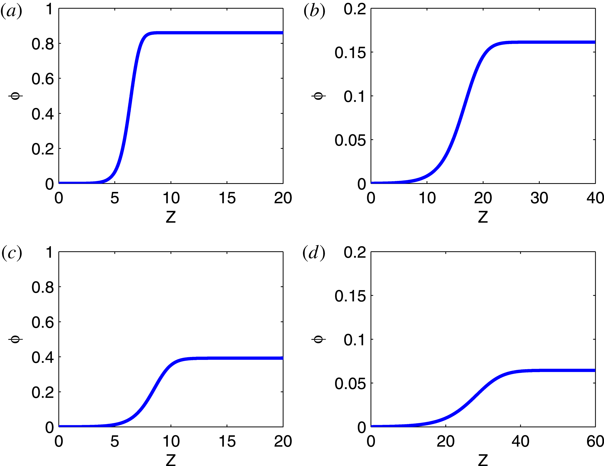
Variation of magnetosonic solitary wave solution given by (3.15) with quantum plasma
 ${\it\beta}_{1}$
as a function of
 $Z$
. Other physical parameters are taken as in case I, i.e.
 $U_{0}=0.6,{\it\delta}={\rm\pi}/15,N_{m}=8,Z_{i}=8,{\it\beta}=0.2814,{\it\Gamma}_{i}=136.5863,{\it\nu}=10$
.

Then we seek the steady-state solution of this KP equation (3.13) in the form
 ${\it\phi}={\it\phi}(Z)$
, where
 $Z=X-UT$
, in which
 $U$
is a constant phase speed. Using this transformation, we can rewrite (3.13) as
 $$\begin{eqnarray}\displaystyle & & \displaystyle (D_{1}\sin ^{2}{\it\delta}-A_{1}U\cos {\it\delta})\frac{\partial {\it\phi}}{\partial Z}+R_{1}\cos ^{2}{\it\delta}{\it\phi}\frac{\partial {\it\phi}}{\partial Z}+C_{1}\cos ^{4}{\it\delta}\frac{\partial ^{3}{\it\phi}}{\partial Z^{3}}\nonumber\\ \displaystyle & & \displaystyle \quad =Q_{1}\cos ^{2}{\it\delta}\int _{-\infty }^{Z}\left(\frac{\partial {\it\phi}}{\partial Z^{\prime }}\right)^{2}\,\text{d}Z^{\prime }.\end{eqnarray}$$
Now using the appropriate boundary conditions, viz,
 ${\it\phi}\rightarrow 0$
,
 $\text{d}{\it\phi}/\text{d}Z\rightarrow 0$
,
 $\text{d}^{2}{\it\phi}/\text{d}Z^{2}\rightarrow 0$
at
 $Z\rightarrow \infty$
, in the absence of
 $Q_{1}$
, a travelling wave solution of (3.14) can be obtained as
 $$\begin{eqnarray}{\it\phi}=\frac{3(A_{1}U\cos {\it\delta}-D_{1}\sin ^{2}{\it\delta})}{R_{1}\cos ^{2}{\it\delta}}\sec h^{2}\left(\sqrt{\frac{A_{1}U\cos {\it\delta}-D_{1}\sin ^{2}{\it\delta}}{4C_{1}\cos ^{4}{\it\delta}}}Z\right),\end{eqnarray}$$
with the assumption
 ${\it\xi}\approx {\it\eta}$
, we give the profiles of the magnetosonic solitons in figures 1 and 2 with the plasma parameters adopted being those used in case I. In figure 1, we explore the effect of the quantum plasma beta,
 ${\it\beta}_{1}$
, on the propagation of the magnetosonic solitary waves. We have
 ${\it\Gamma}_{i}\gg 1$
,
 $155.8774\leqslant {\it\chi}_{e}\leqslant 1892.7$
,
 $0.0051\leqslant {\it\chi}_{i}\leqslant 0.0177$
,
 $9.5355\times 10^{-4}\leqslant {\it\Gamma}_{qe}\leqslant 0.0033$
, which shows that the parameters of degeneracy and the Coulomb coupling parameters are in the kinetic regime. One can see that the amplitude of the magnetosonic solitary waves will decrease while the width will increase with an increase in
 ${\it\beta}_{1}$
. In figure 2, we also investigate the effects of number density ratio of electrons to ions
 ${\it\nu}$
on the soliton structure with the parameters
 $174.1709\leqslant {\it\chi}_{e}\leqslant 438.824$
,
 $0.0043\leqslant {\it\chi}_{i}\leqslant 0.0107$
,
 $0.0020\leqslant {\it\Gamma}_{qe}\leqslant 0.0031$
, which are also in kinetic regime. It is observed that
 ${\it\nu}$
has the same effects as those of
 ${\it\beta}_{1}$
on the propagation of the magnetosonic solitary waves. We mention that an exact analytic solution of (3.13) is very complicated. We can seek an approximate time-dependent solitary solution of (3.13) with a small effect of
 $Q_{1}$
. The strong viscoelastic effects introduce a linear damping of the solitary wave. From the analytical solitary solution, in the absence of viscoelastic effects, one can see that the amplitude and width of the solitary wave both depend on the velocity. Accordingly, we consider the normalized velocity of magnetosonic solitary waves,
 $U$
, is dependent on time
 $T$
,
 $$\begin{eqnarray}{\it\phi}=\frac{3\left[A_{1}U(T)\cos {\it\delta}-D_{1}\sin ^{2}{\it\delta}\right]}{R_{1}\cos ^{2}{\it\delta}}\sec h^{2}\left(\sqrt{\frac{A_{1}U(T)\cos {\it\delta}-D_{1}\sin ^{2}{\it\delta}}{4C_{1}\cos ^{2}{\it\delta}}}Z\right).\end{eqnarray}$$


To determine the time-dependent speed
 $U(T)$
, we use the momentum conservation law in the presence of viscosity as in (Janaki et al.
Reference Janaki, Dasgupta, Gupta and Som1992)
 $$\begin{eqnarray}\frac{\text{d}I}{\text{d}T}=Q_{1}\cos ^{2}{\it\delta}\int _{-\infty }^{+\infty }{\it\phi}\left[\int _{-\infty }^{X}\left(\frac{\partial {\it\phi}}{\partial X^{\prime }}\right)^{2}\,\text{d}X^{\prime }\right]\,\text{d}X,\end{eqnarray}$$
where the momentum of system (3.13) is
 $$\begin{eqnarray}I=\frac{1}{2}\int _{-\infty }^{+\infty }{\it\phi}^{2}\,\text{d}X.\end{eqnarray}$$
Substituting (3.13) into (3.17), we obtain that
 $$\begin{eqnarray}\frac{\text{d}I}{\text{d}T}=Q_{1}\cos ^{2}{\it\delta}\frac{144}{5}\frac{[A_{1}U(T)\cos {\it\delta}-D_{1}\sin ^{2}{\it\delta}]^{3}}{R_{1}^{3}\cos ^{6}{\it\delta}}.\end{eqnarray}$$
Substituting (3.13) into (3.18), we obtain
 $$\begin{eqnarray}I=6\frac{[A_{1}U(T)\cos {\it\delta}-D_{1}\sin ^{2}{\it\delta}]^{2}}{R_{1}^{2}\cos ^{4}{\it\delta}}\sqrt{\frac{4C_{1}\cos ^{4}{\it\delta}}{A_{1}U(T)\cos {\it\delta}-D_{1}\sin ^{2}{\it\delta}}}.\end{eqnarray}$$
Substituting (3.20) into (3.19), one can obtain
 $$\begin{eqnarray}\frac{\text{d}U}{\text{d}T}=\frac{8}{5}\frac{Q_{1}}{A_{1}R_{1}\sqrt{C_{1}}\cos ^{3}{\it\delta}}\left[A_{1}U(T)\cos {\it\delta}-D_{1}\sin ^{2}{\it\delta}\right]^{5/2}.\end{eqnarray}$$
From the above (3.21), we obtain the analytical expression for time-dependent speed as
 $$\begin{eqnarray}U=\frac{D_{1}\sin ^{2}{\it\delta}}{A_{1}\cos {\it\delta}}+\left(U_{0}-\frac{D_{1}\sin ^{2}{\it\delta}}{A_{1}\cos {\it\delta}}\right)\left(1-\frac{T}{T_{0}}\right)^{-2/3},\end{eqnarray}$$
where
 $U_{0}$
is the velocity of the magnetosonic waves when
 $T=0$
and
 $T_{0}$
is given by
 $$\begin{eqnarray}T_{0}=\frac{5R_{1}\sqrt{C_{1}}}{12Q_{1}}\frac{\cos ^{2}{\it\delta}}{(A_{1}U_{0}\cos {\it\delta}-D_{1}\sin ^{2}{\it\delta})^{3/2}}.\end{eqnarray}$$
From the expression for the velocity
 $U(T)$
one can see that the amplitude of the magnetosonic solitary wave decreases slowly with time in the presence of a small ion viscosity
 $Q_{1}$
.
3.2 Shock waves in the hydrodynamic regime
$[{\it\omega}{\it\tau}_{m}\ll 1,{\it\xi},{\it\eta}\sim O({\it\varepsilon})]$

Now we will study the nonlinear propagation of magnetosonic waves in the hydrodynamic regime. Here we note that the dissipation associated with the ion viscosity will play a prominent role in the formation of magnetosonic shock-like waves. Following the same procedure as in the kinetic regime, we will use the lowest expansion given in appendix A. It should be pointed out that the expansions in the hydrodynamic regime are the same as those in the kinetic regime excepting the expansion of (2.16). Accordingly we will use (A 25)–(A 28) instead of (A 4)–(A 5) and (A 16) and (A 17). From the lowest expansion equation in appendix A, one obtains the following equations from the lowest orders of
 ${\it\varepsilon}$
,
 $$\begin{eqnarray}\displaystyle & \displaystyle v_{ix1}=v_{exi}=v_{px1}=E_{y1}=V_{p}B_{z1}, & \displaystyle\end{eqnarray}$$
 $$\begin{eqnarray}\displaystyle & \displaystyle n_{i1}=n_{e1}=n_{p1}=B_{z1}, & \displaystyle\end{eqnarray}$$
 $$\begin{eqnarray}\displaystyle & \displaystyle v_{iy1}=({\it\beta}-V_{p}^{2})\frac{\partial B_{z1}}{\partial {\it\zeta}}-E_{x1}, & \displaystyle\end{eqnarray}$$
 $$\begin{eqnarray}\displaystyle & \displaystyle v_{ey1}=\left(\frac{V_{p}^{2}}{M}-\frac{{\it\beta}_{1}}{3}\right)\frac{\partial B_{z1}}{\partial {\it\zeta}}-E_{x1}, & \displaystyle\end{eqnarray}$$
 $$\begin{eqnarray}\displaystyle & \displaystyle v_{py1}=\left(\frac{{\it\beta}_{2}}{3}-\frac{V_{p}^{2}}{M}\right)\frac{\partial B_{z1}}{\partial {\it\zeta}}-E_{x1}. & \displaystyle\end{eqnarray}$$
 $$\begin{eqnarray}V_{p}^{2}=\frac{1}{1+{\it\gamma}+Z_{i}({\it\nu}+{\it\mu})/M}\left[1+{\it\beta}+\frac{Z_{i}{\it\nu}{\it\beta}_{1}}{3}+\frac{Z_{i}{\it\mu}{\it\beta}_{2}}{3}\right].\end{eqnarray}$$
Finally, eliminating the second-order quantities from the high-order expansions (A 13)–(A 15), (A 18)–(A 24), and (A 27)–(A 28) in the appendix A, namely
 $n_{j2},v_{jy2}$
,
 $v_{jx2},E_{y2},E_{x2}$
and
 $B_{z2}$
, we obtain the KP–Burgers equation as
 $$\begin{eqnarray}\frac{\partial }{\partial {\it\zeta}}\left(A_{2}\frac{\partial {\it\phi}}{\partial {\it\tau}}+R_{2}{\it\phi}\frac{\partial {\it\phi}}{\partial {\it\zeta}}+C_{2}\frac{\partial ^{3}{\it\phi}}{\partial {\it\zeta}^{3}}-D_{2}\frac{\partial ^{2}{\it\phi}}{\partial {\it\zeta}^{2}}\right)+Q_{2}\frac{\partial ^{2}{\it\phi}}{\partial {\it\Gamma}^{2}}=0,\end{eqnarray}$$
where we have also used
 ${\it\phi}=B_{z1}$
for simplicity and the coefficients are given as
 $$\begin{eqnarray}\displaystyle A_{2} & = & \displaystyle \frac{2}{V_{p}}\left(1+{\it\beta}+\frac{Z_{i}{\it\nu}{\it\beta}_{1}}{3}+\frac{Z_{i}{\it\mu}{\it\beta}_{2}}{3}\right),\end{eqnarray}$$
 $$\begin{eqnarray}\displaystyle R_{2} & = & \displaystyle \left[\frac{3Z_{i}({\it\nu}+{\it\mu})}{M}+3\right]V_{p}^{2}-{\it\beta}-\frac{Z_{i}{\it\nu}{\it\beta}_{1}}{9}-\frac{Z_{i}{\it\mu}{\it\beta}_{2}}{9},\end{eqnarray}$$
 $$\begin{eqnarray}\displaystyle C_{2} & = & \displaystyle \frac{Z_{i}{\it\nu}}{M}\left(\frac{V_{p}^{2}}{M}-\frac{{\it\beta}_{1}}{3}\right)^{2}+\frac{Z_{i}{\it\mu}}{M}\left(\frac{V_{p}^{2}}{M}-\frac{{\it\beta}_{2}}{3}\right)^{2}+\frac{1}{Z_{i}^{2}}(V_{p}^{2}-{\it\beta})^{2}\nonumber\\ \displaystyle & & \displaystyle -\,\frac{H^{2}}{4}\frac{Z_{i}({\it\nu}+{\it\mu})}{M}-\frac{1}{1+{\it\gamma}+Z_{i}({\it\nu}+{\it\mu})/M}\left[\frac{Z_{i}{\it\nu}{\it\beta}_{1}}{3M}-\frac{Z_{i}{\it\mu}{\it\beta}_{2}}{3M}\right.\nonumber\\ \displaystyle & & \displaystyle \left.-\,\frac{{\it\beta}}{Z_{1}}+\left(\frac{1}{Z_{i}}-\frac{Z_{i}{\it\nu}}{M^{2}}+\frac{Z_{i}{\it\mu}}{M^{3}}\right)V_{p}^{2}\right]^{2},\end{eqnarray}$$
 $$\begin{eqnarray}\displaystyle D_{2} & = & \displaystyle \bar{{\it\eta}}V_{p},\end{eqnarray}$$
 $$\begin{eqnarray}\displaystyle Q_{2} & = & \displaystyle 1+{\it\beta}+\frac{Z_{i}{\it\nu}{\it\beta}_{1}}{3}+\frac{Z_{i}{\it\mu}{\it\beta}_{2}}{3}.\end{eqnarray}$$
 $\tanh$
method (Malfliet Reference Malfliet2004; Masood, Jehan & Mirza Reference Masood, Jehan and Mirza2010). Accordingly, we unite the independent variables
 ${\it\zeta}$
,
 ${\it\Gamma}$
and
 ${\it\tau}$
into one variable as
 $Z=k({\it\zeta}+{\it\Gamma}-V{\it\tau})$
, where
 $k$
and
 $V$
represents the wavenumber and the travelling velocity of the magnetosonic wave, respectively. Now the KP–Burgers equation (3.30) can be rewritten as
 $$\begin{eqnarray}-k\frac{VA_{2}-Q_{2}}{R_{2}}\frac{\text{d}{\it\phi}}{\text{d}Z}+k{\it\phi}\frac{\text{d}{\it\phi}}{\text{d}Z}+k^{3}\frac{C_{2}}{R_{2}}\frac{\text{d}^{3}{\it\phi}}{\text{d}Z^{3}}-k^{2}\frac{D_{2}}{R_{2}}\frac{\text{d}^{2}{\it\phi}}{\text{d}Z^{2}}=0.\end{eqnarray}$$
By integrating (3.32) once with respect to
 $Z$
with the boundary conditions
 ${\it\phi},\text{d}{\it\phi}/\text{d}Z$
,
 $\text{d}^{2}{\it\phi}/\text{d}Z^{2}\rightarrow 0$
as
 $Z\rightarrow \pm \infty$
, we obtain
 $$\begin{eqnarray}-k\frac{VA_{2}-Q_{2}}{R_{2}}{\it\phi}+\frac{1}{2}k{\it\phi}^{2}+k^{3}\frac{C_{2}}{R_{2}}\frac{\text{d}^{2}{\it\phi}}{\text{d}Z^{2}}-k^{2}\frac{D_{2}}{R_{2}}\frac{\text{d}{\it\phi}}{\text{d}Z}=0.\end{eqnarray}$$
Following the
 $\tanh$
method (Malfliet Reference Malfliet2004; Masood et al.
Reference Masood, Jehan and Mirza2010), we introduce a new variable
 $Y=\tanh (Z)$
. Now the derivative
 $\text{d}/\text{d}Z$
can be replaced by
 $(1-Y^{2})\,\text{d}/\text{d}Y$
. The above (3.33) can be transformed to
 $$\begin{eqnarray}\displaystyle & & \displaystyle -k\frac{VA_{2}-Q_{2}}{R_{2}}{\it\phi}+\frac{1}{2}k{\it\phi}^{2}+k^{3}\frac{C_{2}}{R_{2}}(1-Y^{2})\frac{\text{d}}{\text{d}Y}\left[(1-Y^{2})\frac{\text{d}F(Y)}{\text{d}Y}\right]\nonumber\\ \displaystyle & & \displaystyle \quad -\,k^{2}\frac{D_{2}}{R_{2}}(1-Y^{2})\frac{\text{d}F(Y)}{\text{d}Y}=0.\end{eqnarray}$$
The above (3.34) has a solution of the form
 $$\begin{eqnarray}{\it\phi}(Y)=\frac{3}{25}\frac{D_{2}}{R_{2}C_{2}}(1-Y^{2})+\frac{6}{25}\frac{D_{2}^{2}}{R_{2}C_{2}}(1-Y).\end{eqnarray}$$
If we introduce
 $Y=\tanh (Z)$
into (3.35), the shock wave solution of the KP–Burgers equation (3.30) can be rewritten as
 $$\begin{eqnarray}{\it\phi}=\frac{6}{25}\frac{D_{2}^{2}}{R_{2}C_{2}}\left[1-\tanh \frac{D_{2}}{10C_{2}}({\it\zeta}+{\it\Gamma}-V{\it\tau})\right]+\frac{3}{25}\frac{D_{2}^{2}}{R_{2}C_{2}}\sec h^{2}\frac{D_{2}}{10C_{2}}({\it\zeta}+{\it\Gamma}-V{\it\tau}),\end{eqnarray}$$
with the velocity
 $V=6D_{2}^{2}/(25A_{2}C_{2})+Q_{2}/A_{2}$
and the constant
 $k=D_{2}/10C_{2}$
.
The profiles of the shock solution, which are monotonic in nature, are shown in figure 3. In order to investigate the dependence of the shock waves on plasma parameters, numerical analysis has been performed with the typical parameters given in case II. Here, we choose the dimensionless parameter
 $\bar{{\it\eta}}\approx 1$
. In figure 3(a), we have the parameters
 $65.9099\leqslant {\it\chi}_{e}\leqslant 193.6947$
,
 $0.0287\leqslant {\it\chi}_{i}\leqslant 0.0492$
,
 $0.0298\leqslant {\it\Gamma}_{qe}\leqslant 0.0511$
. Figure 3(a) illustrates that the profiles of the shock waves vary with the value of the quantum plasma
 ${\it\beta}_{1}$
. In figure 3(b) the effects of the number density ratio
 ${\it\nu}$
on the shock waves are illustrated with the parameters
 $8.3546\leqslant {\it\chi}_{e}\leqslant 10.1209$
,
 $0.0088\leqslant {\it\chi}_{i}\leqslant 0.0098$
,
 $0.1304\leqslant {\it\Gamma}_{qe}\leqslant 0.1436$
. It is found that an increase of the quantum plasma beta
 ${\it\beta}_{1}$
, or number density ratio
 ${\it\nu}$
, can lead to a decrease of the amplitudes of the shock waves.
(a) The KP–Burger shock wave structures versus quantum plasma
 ${\it\beta}_{1}$
, where the parameters are taken as those in case II, i.e.
 $N_{m}=8,Z_{i}=1,{\it\beta}=0.0517,{\it\nu}=10,{\it\Gamma}_{i}=5.7930,\bar{{\it\eta}}\approx 1$
. (b) The KP–Burger shock wave structures versus number density ratio
 ${\it\nu}$
and physical parameters are taken as
 ${\it\beta}_{1}=0.1570$
and the others are the same as in (a).

The numerical solution of shock waves (a)
 ${\it\beta}_{1}=0.3,{\it\nu}=10$
; (b)
 ${\it\beta}_{1}=0.3,{\it\nu}=20$
; (c)
 ${\it\beta}_{1}=0.6,{\it\nu}=10$
; and (d)
 ${\it\beta}_{1}=0.6,{\it\nu}=20$
.

We also numerically investigate the travelling wave solution of the KP–Burger equation (3.30) with the same plasma parameters as those in figure 3. In a comoving coordinate
 $Z={\it\zeta}+{\it\Gamma}-V_{0}{\it\tau}$
, where
 $V_{0}$
is the constant velocity of the shock waves, the KP–Burger equation (3.36) reduces to a third-order ordinary differential equation. By integrating (3.36) once with respect to
 $Z$
, with the boundary conditions
 ${\it\phi}$
,
 $\text{d}{\it\phi}/\text{d}Z$
,
 $\text{d}^{2}{\it\phi}/\text{d}Z^{2}\rightarrow 0$
as
 $Z\rightarrow \pm \infty$
, we obtain
 $$\begin{eqnarray}C_{2}\frac{\text{d}^{2}{\it\phi}}{\text{d}Z^{2}}-D_{2}\frac{\text{d}{\it\phi}}{\text{d}Z}-(A_{2}V_{0}-Q_{2}){\it\phi}+\frac{R_{2}}{2}{\it\phi}^{2}=0.\end{eqnarray}$$
By introducing
 $\text{d}{\it\phi}/\text{d}Z={\it\psi}$
, (3.37) can be rewritten as
 $$\begin{eqnarray}\left.\begin{array}{@{}c@{}}\displaystyle \frac{\text{d}{\it\phi}}{\text{d}Z}={\it\psi},\\ \displaystyle \frac{\text{d}{\it\psi}}{\text{d}Z}=\frac{D_{2}}{C_{2}}{\it\psi}+\frac{A_{2}V_{0}-Q_{2}}{C_{2}}{\it\phi}-\frac{R_{2}}{2C_{2}}{\it\phi}^{2}.\end{array}\right\}\end{eqnarray}$$
In the
 $[{\it\phi},{\it\psi}]$
plane, (3.38) has two singular points, namely
 $[0,0]$
and
 $[2(A_{2}V_{0}-Q_{2})/R_{2},0]$
. The former is a saddle point corresponding to the equilibrium downstream state. The nature of the latter (corresponding to the upstream state) can be determined from the asymptotic behaviour of the solution of the form
 ${\sim}\exp ({\it\alpha}Z)$
of the linearized (3.37) with the parameters
 $$\begin{eqnarray}{\it\alpha}=\frac{1}{2C_{2}}[D_{2}\pm \sqrt{D_{2}^{2}+4C_{2}(A_{2}V_{0}-Q_{2})}].\end{eqnarray}$$
Thus the singular point is a stable node for
 $D_{2}^{2}+4C_{2}(A_{2}V_{0}-Q_{2})>0$
or a stable focus for
 $D_{2}^{2}+4C_{2}(A_{2}V_{0}-Q_{2})<0$
, which corresponds to a monotonic shock front and an oscillatory profile, respectively. We note that for the parameters relevant for case II the condition
 $D_{2}^{2}+4C_{2}(A_{2}V_{0}-Q_{2})>0$
holds good. If one chooses the velocity as that of the steady shock wave solution
 $V_{0}=6D_{2}^{2}/(25A_{2}C_{2})+Q_{2}/A_{2}$
obtained from the
 $\tanh$
method (Malfliet Reference Malfliet2004; Masood et al.
Reference Masood, Jehan and Mirza2010), the stable node
 $D_{2}^{2}+4C_{2}(A_{2}V_{0}-Q_{2})=(49/25)D_{2}^{2}>0$
always holds well. We numerically solve (3.38) by the standard fourth-order Runge–Kutta scheme with a step size
 ${\rm\Delta}Z=0.001$
considering the parameters in case II. The results are shown in figure 4, in which only monotonic shock waves occur. The left column in figure 4 shows results for number density ratio
 ${\it\nu}=10$
and the right for number density ratio
 ${\it\nu}=20$
, which shows that the shock height increases with a decrease in the number density ratio
 ${\it\nu}$
. The upper panel plots (a) and (b) are for the same quantum plasma beta
 ${\it\beta}_{1}=0.35$
and the lower panel plots (c) and (d) are for the same quantum plasma beta
 ${\it\beta}_{1}=0.6$
. Then one can see that the height of the shock waves decrease with the quantum diffraction effects increasing. We can conclude that the shock solution is always stable as the singular point is always a stable node, which is confirmed by figure 4.
4 Conclusion
Two-dimensional nonlinear magnetosonic waves propagating perpendicular to the applied magnetic field
 $\boldsymbol{B}_{0}=B_{0}\hat{\boldsymbol{e}}_{z}$
have been investigated in a collisionless, strongly coupled quantum EPI plasma. The generalized viscoelastic model with the effects of electrostatic ion pressure due to strong coupling of the ions and a quantum hydrodynamic model with the effects of the quantum force associated with the Bohm potential and the quantum statistic degeneracy pressure of electrons and positrons are used for ions and electrons (positrons), respectively. In the weak nonlinearity limit, a mKP equation and a KP–Burger equation have been derived in the kinetic regime
 ${\it\omega}{\it\tau}_{m}\gg 1$
and hydrodynamic regime
 ${\it\omega}{\it\tau}_{m}\ll 1$
respectively.
In the kinetic regime, the low-frequency magnetosonic kinetic wave modes may propagate as solitary waves, of which the amplitude decreases with time due to the ion viscosity. It is observed that the amplitude of the magnetosonic solitary waves will decrease while the width will increase with an increase of the quantum plasma beta
 ${\it\beta}_{1}$
and number density ratio
 ${\it\nu}$
. We also give an approximate soliton solution of the mKP equation by using the momentum conservation law. The analytical solution shows that the amplitude of the solitary waves are reduced with time. In the hydrodynamic regime, the low-frequency magnetosonic hydrodynamic wave modes propagate as shock waves when one considers that the ion coupling parameter
 ${\it\Gamma}_{i}$
is in the range of
 $1\sim 10$
. Both the analytical and numerical results show that an increase of the quantum plasma beta
 ${\it\beta}_{1}$
, or number density ratio
 ${\it\nu}$
, can lead to a decrease of the amplitude of the shock waves.
Acknowledgements
This work is supported by the National Natural Science Foundation of China (no. 11104012) and the Fundamental Research Funds for the Central Universities (nos FRF-TP-09-019A, FRF-BR-11-031B).
Appendix A
The lowest-order expansions of (2.15)–(2.20) are given in the kinetic regime as
 $$\begin{eqnarray}\displaystyle & \displaystyle -V_{p}\frac{\partial n_{i1}}{\partial {\it\zeta}}+\frac{\partial v_{ix1}}{\partial {\it\zeta}}=0, & \displaystyle\end{eqnarray}$$
 $$\begin{eqnarray}\displaystyle & \displaystyle -V_{p}\frac{\partial n_{e1}}{\partial {\it\zeta}}+\frac{\partial v_{ex1}}{\partial {\it\zeta}}=0, & \displaystyle\end{eqnarray}$$
 $$\begin{eqnarray}\displaystyle & \displaystyle -V_{p}\frac{\partial n_{p1}}{\partial {\it\zeta}}+\frac{\partial v_{px1}}{\partial {\it\zeta}}=0, & \displaystyle\end{eqnarray}$$
 $$\begin{eqnarray}\displaystyle & \displaystyle {\it\tau}_{m}V_{p}^{2}\frac{\partial ^{2}v_{ix1}}{\partial {\it\zeta}^{2}}+Z_{i}{\it\tau}_{m}V_{p}\frac{\partial E_{x1}}{\partial {\it\zeta}}+Z_{i}{\it\tau}_{m}V_{p}\frac{\partial v_{iy1}}{\partial {\it\zeta}}-{\it\beta}{\it\tau}_{m}V_{p}\frac{\partial ^{2}n_{i1}}{\partial {\it\zeta}^{2}}-\left({\it\xi}+\frac{4}{3}{\it\eta}\right)\frac{\partial ^{2}v_{ix1}}{\partial {\it\zeta}^{2}}=0, & \displaystyle\end{eqnarray}$$
 $$\begin{eqnarray}\displaystyle & \displaystyle \frac{\partial E_{y1}}{\partial {\it\zeta}}-\frac{\partial v_{ix1}}{\partial {\it\zeta}}=0, & \displaystyle\end{eqnarray}$$
 $$\begin{eqnarray}\displaystyle & \displaystyle v_{ex1}-E_{y1}=0, & \displaystyle\end{eqnarray}$$
 $$\begin{eqnarray}\displaystyle & \displaystyle V_{p}\frac{\partial v_{ex1}}{\partial {\it\zeta}}-ME_{x1}-Mv_{ey1}-\frac{1}{3}{\it\beta}_{1}M\frac{\partial n_{e1}}{\partial {\it\zeta}}=0, & \displaystyle\end{eqnarray}$$
 $$\begin{eqnarray}\displaystyle & \displaystyle v_{px1}-E_{y1}=0, & \displaystyle\end{eqnarray}$$
 $$\begin{eqnarray}\displaystyle & \displaystyle V_{p}\frac{\partial v_{px1}}{\partial {\it\zeta}}+ME_{x1}+Mv_{py1}-\frac{1}{3}{\it\beta}_{2}M\frac{\partial n_{p1}}{\partial {\it\zeta}}=0, & \displaystyle\end{eqnarray}$$
 $$\begin{eqnarray}\displaystyle & \displaystyle {\it\nu}v_{ex1}-{\it\mu}v_{px1}-v_{ix1}=0, & \displaystyle\end{eqnarray}$$
 $$\begin{eqnarray}\displaystyle & \displaystyle {\it\gamma}V_{p}\frac{\partial E_{y1}}{\partial {\it\zeta}}-\frac{\partial B_{z1}}{\partial {\it\zeta}}+Z_{i}{\it\nu}v_{ey1}-Z_{i}{\it\mu}v_{py1}-Z_{i}v_{iy1}=0, & \displaystyle\end{eqnarray}$$
 $$\begin{eqnarray}\displaystyle & \displaystyle \frac{\partial E_{y1}}{\partial {\it\zeta}}-V_{p}\frac{\partial B_{z1}}{\partial {\it\zeta}}=0. & \displaystyle\end{eqnarray}$$
 $$\begin{eqnarray}\displaystyle & \displaystyle -V_{p}\frac{\partial n_{i2}}{\partial {\it\zeta}}+\frac{\partial n_{i1}}{\partial {\it\tau}}+\frac{\partial v_{ix2}}{\partial {\it\zeta}}+\frac{\partial n_{i1}v_{ix1}}{\partial {\it\zeta}}+\frac{\partial v_{iy1}}{\partial {\it\Gamma}}=0, & \displaystyle\end{eqnarray}$$
 $$\begin{eqnarray}\displaystyle & \displaystyle -V_{p}\frac{\partial n_{e2}}{\partial {\it\zeta}}+\frac{\partial n_{e1}}{\partial {\it\tau}}+\frac{\partial v_{ex2}}{\partial {\it\zeta}}+\frac{\partial n_{e1}v_{ex1}}{\partial {\it\zeta}}+\frac{\partial v_{ey1}}{\partial {\it\Gamma}}=0, & \displaystyle\end{eqnarray}$$
 $$\begin{eqnarray}\displaystyle & \displaystyle -V_{p}\frac{\partial n_{p2}}{\partial {\it\zeta}}+\frac{\partial n_{p1}}{\partial {\it\tau}}+\frac{\partial v_{px2}}{\partial {\it\zeta}}+\frac{\partial n_{p1}v_{px1}}{\partial {\it\zeta}}+\frac{\partial v_{py1}}{\partial {\it\Gamma}}=0, & \displaystyle\end{eqnarray}$$
 $$\begin{eqnarray}\displaystyle & \displaystyle {\it\tau}_{m}V_{p}^{2}\frac{\partial ^{2}v_{ix2}}{\partial {\it\zeta}^{2}}-{\it\tau}_{m}V_{p}\frac{\partial ^{2}v_{ix1}}{\partial {\it\zeta}\partial {\it\tau}}-{\it\tau}_{m}V_{p}\left[\left(\frac{\partial v_{ix1}}{\partial {\it\zeta}}\right)^{2}+v_{ix1}\frac{\partial ^{2}v_{ix1}}{\partial {\it\zeta}^{2}}\right]\hspace{56.9055pt} & \displaystyle \nonumber\\ \displaystyle & \displaystyle \hspace{19.91684pt}+\,Z_{i}{\it\tau}_{m}V_{p}\left[\frac{\partial E_{x2}}{\partial {\it\zeta}}+\frac{\partial v_{iy2}}{\partial {\it\zeta}}+\frac{\partial v_{iy1}B_{z1}}{\partial {\it\zeta}}+\frac{\partial n_{i1}(E_{x1}+v_{iy1})}{\partial {\it\zeta}}-{\it\beta}\frac{\partial ^{2}n_{i2}}{\partial {\it\zeta}^{2}}\right] & \displaystyle \nonumber\\ \displaystyle & \displaystyle \hspace{11.38092pt}-\,{\it\tau}_{m}V_{p}\left(\frac{\partial ^{2}v_{ix1}}{\partial {\it\zeta}\partial {\it\tau}}+v_{ix1}\frac{\partial ^{2}v_{ix1}}{\partial {\it\zeta}^{2}}\right)+{\it\tau}_{m}V_{p}^{2}\left(\frac{\partial n_{i1}}{\partial {\it\zeta}}\frac{\partial v_{ix1}}{\partial {\it\zeta}}+n_{i1}\frac{\partial ^{2}v_{ix1}}{\partial {\it\zeta}^{2}}\right) & \displaystyle \nonumber\\ \displaystyle & \displaystyle \hspace{45.52458pt}+\,{\it\tau}_{m}{\it\beta}\left(\frac{\partial ^{2}n_{i1}}{\partial {\it\zeta}\partial {\it\tau}}+v_{ix1}\frac{\partial ^{2}n_{i1}}{\partial {\it\zeta}^{2}}\right)-{\it\tau}_{m}Z_{i}\left[\frac{\partial (E_{x1}+v_{iy1})}{\partial {\it\tau}}+v_{ix1}\frac{\partial (E_{x1}+v_{iy1})}{\partial {\it\zeta}}\right] & \displaystyle \nonumber\\ \displaystyle & \displaystyle \hspace{-58.79993pt}=\left({\it\xi}+\frac{4}{3}{\it\eta}\right)\frac{\partial ^{2}v_{ix2}}{\partial {\it\zeta}^{2}}+{\it\eta}\frac{\partial ^{2}v_{ix1}}{\partial {\it\Gamma}^{2}}+\left({\it\xi}+\frac{{\it\eta}}{3}\right)\frac{\partial ^{2}v_{iy1}}{\partial {\it\zeta}\partial {\it\Gamma}}, & \displaystyle\end{eqnarray}$$
 $$\begin{eqnarray}\displaystyle & \displaystyle \hspace{4.0pt}-{\it\tau}_{m}V_{p}\left[{\it\beta}\frac{\partial ^{2}n_{i1}}{\partial {\it\zeta}\partial {\it\Gamma}}-Z_{i}\frac{\partial E_{y2}}{\partial {\it\zeta}}+Z_{i}\frac{\partial v_{ix2}}{\partial {\it\zeta}}+Z_{i}\frac{\partial v_{ix1}B_{z1}}{\partial {\it\zeta}}+Z_{i}\frac{\partial n_{i1}(v_{ix1}-E_{y1})}{\partial {\it\zeta}}\right] & \displaystyle \nonumber\\ \displaystyle & \displaystyle +\,{\it\tau}_{m}\left[V_{p}^{2}\frac{\partial ^{2}v_{iy1}}{\partial {\it\zeta}^{2}}+Z_{i}\frac{\partial (v_{ix1}-E_{y1})}{\partial {\it\tau}}+Z_{i}v_{ix1}\frac{\partial (v_{ix1}-E_{y1})}{\partial {\it\zeta}}\right]\hspace{19.91684pt} & \displaystyle \nonumber\\ \displaystyle & \displaystyle \hspace{-68.39996pt}={\it\eta}\frac{\partial ^{2}v_{iy1}}{\partial {\it\zeta}^{2}}+\left({\it\xi}+\frac{{\it\eta}}{3}\right)\frac{\partial ^{2}v_{ix1}}{\partial {\it\zeta}\partial {\it\Gamma}},\hspace{79.6678pt} & \displaystyle\end{eqnarray}$$
 $$\begin{eqnarray}\displaystyle & \displaystyle V_{p}\frac{\partial v_{ex2}}{\partial {\it\zeta}}-\frac{\partial v_{ex1}}{\partial {\it\tau}}-v_{ex1}\frac{\partial v_{ex1}}{\partial {\it\zeta}}-ME_{x2}-M(v_{ey2}+v_{ey1}B_{z1}) & \displaystyle \nonumber\\ \displaystyle & \displaystyle -\,\frac{1}{3}{\it\beta}_{1}M\left(\frac{\partial n_{e2}}{\partial {\it\zeta}}-\frac{1}{3}n_{e1}\frac{\partial n_{e1}}{\partial {\it\zeta}}\right)+\frac{H^{2}}{4}\frac{\partial ^{3}n_{e1}}{\partial {\it\zeta}^{3}}=0, & \displaystyle\end{eqnarray}$$
 $$\begin{eqnarray}\displaystyle & \displaystyle V_{p}\frac{\partial v_{ey1}}{\partial {\it\zeta}}-M(E_{y2}-v_{ex1}B_{z1}-v_{ex2})-\frac{1}{3}{\it\beta}_{1}M\frac{\partial n_{e1}}{\partial {\it\Gamma}}=0, & \displaystyle\end{eqnarray}$$
 $$\begin{eqnarray}\displaystyle & \displaystyle V_{p}\frac{\partial v_{px2}}{\partial {\it\zeta}}-\frac{\partial v_{px1}}{\partial {\it\tau}}-v_{px1}\frac{\partial v_{px1}}{\partial {\it\zeta}}+ME_{x2}+M(v_{px2}+v_{py1}B_{z1}) & \displaystyle \nonumber\\ \displaystyle & \displaystyle -\,\frac{1}{3}{\it\beta}_{2}M\left(\frac{\partial n_{p2}}{\partial {\it\zeta}}-\frac{1}{3}n_{p1}\frac{\partial n_{p1}}{\partial {\it\zeta}}\right)+\frac{H^{2}}{4}\frac{\partial ^{3}n_{p1}}{\partial {\it\zeta}^{3}}=0, & \displaystyle\end{eqnarray}$$
 $$\begin{eqnarray}\displaystyle & \displaystyle V_{p}\frac{\partial v_{py1}}{\partial {\it\zeta}}+M(E_{y2}-v_{px1}B_{z1}-v_{px2})-\frac{1}{3}{\it\beta}_{2}M\frac{\partial n_{p1}}{\partial {\it\Gamma}}=0, & \displaystyle\end{eqnarray}$$
 $$\begin{eqnarray}\displaystyle & \displaystyle \frac{\partial B_{z1}}{\partial {\it\Gamma}}+{\it\gamma}V_{p}\frac{\partial E_{x1}}{\partial {\it\zeta}}+Z_{i}{\it\nu}(v_{ex2}+n_{e1}v_{ex1})-Z_{i}{\it\mu}(v_{px2}+n_{p1}v_{px1})-Z_{i}(v_{ix2}+n_{i1}v_{ix1})=0, & \displaystyle \nonumber\\ \displaystyle & & \displaystyle\end{eqnarray}$$
 $$\begin{eqnarray}\displaystyle & \displaystyle {\it\gamma}V_{p}\frac{\partial E_{y2}}{\partial {\it\zeta}}-\frac{\partial E_{y1}}{\partial {\it\tau}}-\frac{\partial B_{z2}}{\partial {\it\zeta}}+Z_{i}{\it\nu}(v_{ey2}+n_{e1}v_{ey1})-Z_{i}{\it\mu}(v_{py2}+n_{p1}v_{py1}) & \displaystyle \nonumber\\ \displaystyle & \displaystyle -\,Z_{i}(v_{iy2}+n_{i1}v_{iy1})=0, & \displaystyle\end{eqnarray}$$
 $$\begin{eqnarray}\displaystyle & \displaystyle \frac{\partial E_{y2}}{\partial {\it\zeta}}-V_{p}\frac{\partial B_{z2}}{\partial {\it\zeta}}-\frac{\partial E_{x1}}{\partial {\it\Gamma}}+\frac{\partial B_{z1}}{\partial {\it\tau}}=0. & \displaystyle\end{eqnarray}$$
 $$\begin{eqnarray}\displaystyle & \displaystyle -V_{p}\frac{\partial v_{ix1}}{\partial {\it\zeta}}-Z_{i}(E_{x1}+v_{iy1})+{\it\beta}\frac{\partial n_{i1}}{\partial {\it\zeta}}=0, & \displaystyle\end{eqnarray}$$
 $$\begin{eqnarray}\displaystyle & \displaystyle v_{ix1}-E_{y1}=0. & \displaystyle\end{eqnarray}$$
 $$\begin{eqnarray}\displaystyle & \displaystyle -V_{p}n_{i1}\frac{\partial v_{ix1}}{\partial {\it\zeta}}-V_{p}\frac{\partial v_{ix2}}{\partial {\it\zeta}}+\frac{\partial v_{ix1}}{\partial {\it\tau}}+v_{ix1}\frac{\partial v_{ix1}}{\partial {\it\zeta}}-Z_{i}n_{i1}(E_{x1}+v_{iy1}) & \displaystyle \nonumber\\ \displaystyle & \displaystyle -\,Z_{i}(E_{x2}+v_{iy1}B_{z1}+v_{iy2})+{\it\beta}\frac{\partial n_{i2}}{\partial {\it\zeta}}=\left({\it\xi}+\frac{4}{3}{\it\eta}\right)\frac{\partial ^{2}v_{ix1}}{\partial {\it\zeta}^{2}}, & \displaystyle\end{eqnarray}$$
 $$\begin{eqnarray}\displaystyle & \displaystyle -V_{p}\frac{\partial v_{iy1}}{\partial {\it\zeta}}-Z_{i}E_{y2}+Z_{i}v_{ix2}+{\it\beta}\frac{\partial n_{i1}}{\partial {\it\Gamma}}+Z_{i}v_{ix1}B_{z1}-Z_{i}n_{i1}(E_{y1}-v_{ix1})=0. & \displaystyle\end{eqnarray}$$