Introduction
In modern telecommunications technology, the studies of radio frequency (RF) power amplifiers (PAs) have become more attractive for RF engineers, since the performance of wireless systems strongly depends on the quality of RF PAs in terms of power efficiency and linearity [Reference Ghannouchi, Hammi and Helaoui1]. These criteria are more significant in (massive) multiple-input multiple-output (MIMO) systems [Reference Larsson, Edfors, Tufvesson and Marzetta2,Reference Abdelaziz, Anttila and Valkama3]. Hence, most attempts are dedicated to reducing the consequences of major impairments of RF PAs.
An amplifier can be driven to operate close to its saturation region to increase its power efficiency, but it consequently causes a non-linearity effect, and spectral deficiency dissipating spectral powers in out-of-band regions; power efficiency and spectral efficiency cannot be achieved simultaneously [Reference Ghannouchi, Hammi and Helaoui1]. The memory effect is the other major shortcoming of RF PAs excited by wideband signals, e.g. orthogonal frequency division multiplexing (OFDM) and wideband code division multiple access (WCDMA), degrading the performance of PAs [Reference Vuolevi and Rahkonen4,Reference Pedro and Mass5]. The effects of input and output cross-talks in MIMO transmitters cause additional impairments [Reference Bassam, Helaoui and Ghannouchi6].
Volterra theory is mathematically a powerful tool to describe the behavior of weakly non-linear dynamic systems with fading memory [Reference Schetzen7]. In practice, polynomial-type and black-box models, which are reduced forms of the Volterra model, are preferred [Reference Ghannouchi, Hammi and Helaoui1,Reference Wood8] to improve the performance in terms of computational complexity and accuracy for modeling strong non-linear systems with long-memory effects [Reference Mathews and Sicuranza9].
Several techniques have been proposed in the time domain to mitigate the impairments of RF PAs in MIMO systems. In [Reference Bassam, Helaoui and Ghannouchi6], a cross-over digital pre-distortion technique consisting of two parallel Hammerstein (PH) models was investigated to compensate the effects of the input cross-talk and non-linearity of RF PAs in a MIMO system. A two-dimensional (2D) generalized memory polynomial (GMP) model was studied in [Reference Amin, Landin, Händel and Rönnow10] for modeling and linearizing RF PAs in a MIMO system including input and output cross-talks. However, in a K × K MIMO system where K>2, a 2D model will not be efficient for modeling or linearising the distortion of PAs, since the effect of cross-talks are caused by two or more neighborhood channels. In [Reference Alizadeh, Amin and Rönnow11], the 3rd-order Volterra self- and cross-kernels of PAs were analyzed in the frequency domain using a three-tone test and their main block structures were determined in a 3 × 3 MIMO system including input cross-talk channels. Furthermore, in [Reference Khan, Zenteno, Händel and Isaksson12] the frequency-domain analyses of the 3rd-order Volterra kernels of PAs were investigated using multi-tones signals in a 3 × 3 MIMO system including input and output cross-talks. Using multi-tones excitation signal is more practical to analyze the behavior of PAs within the whole signal bandwidth. Although the analyses and experimental performances of the works in [Reference Alizadeh, Amin and Rönnow11,Reference Khan, Zenteno, Händel and Isaksson12] are cumbersome and limited to the 3rd-order kernels, they could be useful to formulate the structure of MIMO models for PAs [Reference Alizadeh, Rönnow, Händel and Isaksson13]. A higher dimensional model was also investigated in [Reference Hausmair, Landin, Gustavsson, Fager and Eriksson14] that proposed a simplified 4D dual-input memory polynomial DPD to consider the linear effects of antenna cross-talk and impedance mismatch for non-linear RF PAs in a MIMO system. However, the input cross-talk effects were not examined and the excitation signals were relatively narrowband, which may affect the performance and computational complexity of the model. Recent studies have investigated massive MIMO systems. A PH model was used in [Reference Abdelaziz, Anttila and Valkama3] to compensate the simulated impairments of RF PAs for a massive MIMO application, whereas the output cross-talk effects were not considered.
Frequency-domain modeling techniques have also been investigated for decades. In [Reference Chiu, Zeng and Liu15], a frequency-domain pre-distorter was proposed for identifying the parameters of a non-linear static single-input single-output (SISO) model using the zero-forcing (ZF) and adaptive least squares (LS) techniques, whereas it is not suitable for dynamic system. The frequency-domain piece-wise fitting approach was also used to estimate poles and zeros of the transfer function of a SISO system within several sub-bands [Reference Zhang and Xie16] in an LS sense. However, it was also assumed that the transfer function of the system is directly measurable.
Contributions
In this paper, firstly, a time-domain 3D GMP model is proposed for RF PAs in a 3 × 3 MIMO system including both input and output cross-talk channels. The model is an extension of the 2D GMP model in [Reference Amin, Landin, Händel and Rönnow10]. A 2D model cannot be directly used for modeling the cross-talk effects of neighborhood channels coming from different sides in higher dimensional systems. Depending on the system configuration and topology, each channel is surrounded by two or more neighborhood channels. Since, the significance of cross-talk effects are limited in the vicinity of each channel, a higher dimensional (i.e. massive MIMO) model can be reduced to a lower dimension, e.g. 3D or 4D. The major drawbacks of the conventional time-domain modeling technique for MIMO systems are the large dimensionality of the model and the increased computational complexity. Hence, secondly, a 3D frequency-domain technique is also proposed for RF PAs in MIMO systems based on the 3D time-domain modeling technique. In this technique, the bandwidth of the system is divided into several sub-bands, and a curve fitting approach [Reference Zhang and Xie16,Reference Zhao, Hao, Alomainy and Parini17] is used to estimate the parameters for each sub-band. However, the transfer function is unknown in this technique and is estimated by incorporating the frequency-domain input and output samples into the curve fitting approach. The sub-band estimation technique has some advantages compared to conventional frequency-domain modeling techniques [Reference Chiu, Zeng and Liu15]. Since the bandwidth of a sub-band is much narrower than the entire bandwidth of the system, the number of parameters for each sub-band is reduced, and hence the total computational complexity. The bandwidth of sub-bands can be searched to find an optimal performance in terms of the minimum normalized mean square error (NMSE), adjacent channel error power ratio (ACEPR) and adjacent channel leakage ratio (ACLR) criteria. The proposed frequency-domain technique could be useful to reduce the complexity of digital pre-distorters in massive MIMO systems, and in very wideband, e.g. millimetre-wave, applications [Reference Zhang and Chen18,Reference Liu, Pan and Shao19].
The structure of this paper is organized as follows. The section “Model description” describes the theory of time- and frequency-domain behavioral modeling techniques for RF PAs in MIMO systems. The identification and evaluation techniques are explained in the section “Model identification”. The section “Experimental setup” explains the experimental setup. The measurement results of two techniques are presented and discussed for behavioral modeling and DPD techniques in the section “Results”. The discussion and conclusion are given in the section “Discussion”, and the section “Conclusion”, respectively.
Model description
Model prerequisites
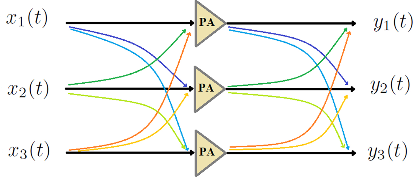
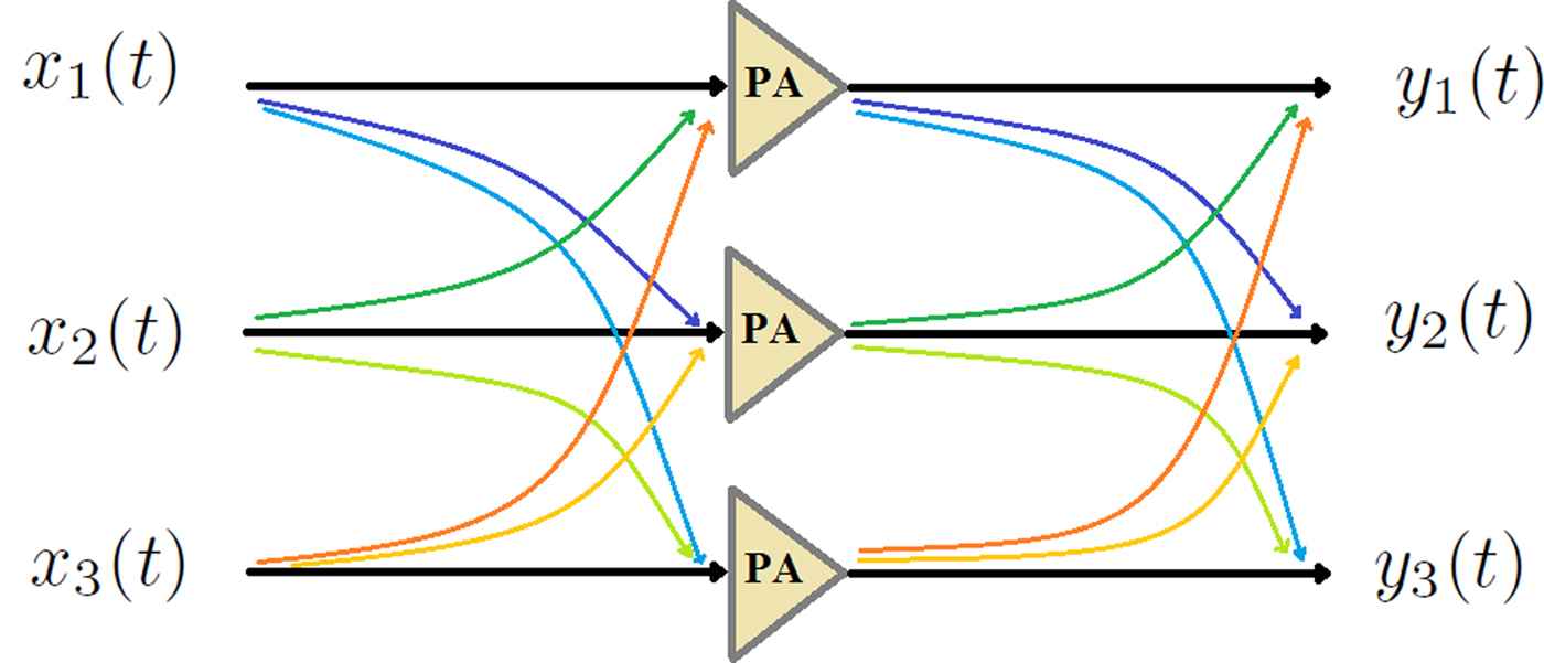
Figure 1 shows a 3 × 3 MIMO system consisting of input cross-talk channels, RF PAs, and output cross-talk channels. The input cross-talk effects are caused by a common oscillator for up-converting baseband signals, and transmission lines, e.g. cables and microstrip lines before PAs. The RF PAs are usually operating close to their saturation regions to achieve a higher power efficiency, and consequently, cause distortions and non-linearity effects. Furthermore, RF PAs show memory effects that degrade the performance. The output cross-talk effects are caused by coupled microstrip lines, and antennas. Both input and output cross-talk channels may show some memory effects. The effects of input cross-talk will contribute to non-linearity effects of PAs, whereas the output cross-talks have linear effects under an output impedance matched condition [Reference Bassam, Helaoui and Ghannouchi6], but in the case of an impedance mismatch condition, the non-linear effects of output cross-talks should be considered [Reference Hausmair, Landin, Gustavsson, Fager and Eriksson14, Reference Zargar, Banai and Pedro20].
A 3 × 3 MIMO system including input and output cross-talk channels.
System model
The relations between the input and output signals at the RF frequency region in the presence of the input and output cross-talks in a 3 × 3 MIMO system are given as
 $$ \eqalign{y_\ell(t) &= \, \beta_{\ell1}(t) * f_1 \big( (\alpha_{11} * x_{1} )(t)+ (\alpha_{12} * x_{2})(t) + (\alpha_{13} * x_{3})(t) \big) \cr & + \beta_{\ell2}(t) * f_2 \big( (\alpha_{21} *x_{1})(t) + (\alpha_{22} * x_{2}) (t)+ (\alpha_{23} * x_{3})(t) \big) \cr & + \beta_{\ell3}(t) * f_3 \big( (\alpha_{31} *x_{1} ) (t)+ (\alpha_{32} * x_{2}) (t)+ (\alpha_{33} * x_{3})(t) \big),} $$
where x ℓ; ℓ = 1, 2, 3 and y ℓ indicate the ℓth input and output signals, respectively, and f ℓ( · ) is the non-linear dynamic operator of the ℓth PA. In general, αℓm(t) and βℓm(t) are impulse responses describing the dynamic models of the input and output cross-talk effects from the mth channel on the ℓth channel, respectively, and “*" indicates a convolution operator. In the case of symmetric and static cross-talk channels, the structures of the model can be simplified [Reference Vejdani Amiri, Helaoui and Ghannouchi21].
In this work, a 3D GMP model is proposed for a 3 × 3 MIMO system including input and output cross-talk channels (shown in Fig. 1). First, the discrete time-domain complex baseband model is established, and then the discrete frequency-domain complex baseband model is defined based on the time-domain model.
Time-domain modeling via 3D GMP
When there are no input and output cross-talk effects, a 3 × 3 MIMO system can be modeled by three independent SISO models, e.g. a generalized memory polynomial (GMP) model [Reference Morgan, Ma, Kim, Zierdt and Pastalan22] of a non-linear SISO system including lagging cross-terms is given by
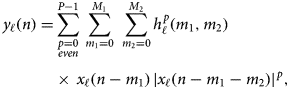 $$ \eqalign{ y_\ell(n) = & \mathop \sum \limits_{\scriptstyle p = 0 \atop \scriptstyle even } ^{P-1} \, \mathop \sum \limits_{m_1 = 0}^{M_1} \,\, \mathop \sum \limits_{m_2 = 0}^{M_2} h^{\,p}_{\ell}(m_1,m_2) \cr &\times \, x_\ell(n-m_1) \, \vert x_\ell(n-m_1-m_2)\vert ^{\,p}, } $$
where x ℓ(n) and y ℓ(n); ℓ = 1, 2, 3 are the input and output of the ℓth channel of the system, respectively. Furthermore, P is the highest order of non-linearity in the model, M 1 is the memory length along diagonal terms, M 2 is a deviation from diagonal terms representing memories along cross-terms, and  $h^{p}_{\ell }(m_1,m_2)$ is the parameter of the (1 + p)th-order system. In total, there are (1 + P) (1 + M 1) (1 + M 2)/2 parameters in the model. In the special case when M 2 = 0, the model in (2) reduces to a memory polynomial (MP) [Reference Kim and Konstantinou23] model, which only characterizes the memory effects of the system along diagonal terms.
With (2) as a starting point, a matrix formulation reads as
 $$ {\bf y}_\ell = {\bf X}_{\ell} {\bf h}_{\ell}, $$
where yℓ denotes the vector of N samples of y ℓ(n).
 $ {\bf h_{\ell }} = [h^{0}_{\ell }(0,0) \, \ldots \, h^{P-1}_{\ell }(M_1,M_2)]^T$ is the vector of parameters in (3). Xℓ denotes the regression matrix for the ℓth input signal. Generalizing, the equation above provides us with the 3D GMP model, and the output signal at the ℓth channel is given as
 $$ \eqalign{ y_\ell(n) & = \! \sum\limits_{m_1 = 0}^{M_1} {\sum\limits_{m_2 = 0}^{M_2} {\mathop \sum \limits_{\scriptstyle p = 0 \atop \scriptstyle {\rm even} } ^{P-1} } } \bigg[ h^{\,p,0,0}_{\ell,1,1,1}(m_1,m_2) \, x_1(n\! - \!m_1) \,\vert x_1(n \! - \! m_1 \! - \! m_2)\cr &\vert ^{\,p} + \mathop \sum \limits_{\scriptstyle q = 0 \atop \scriptstyle {\rm even} } ^{P-p} h^{\,p,q,0}_{\ell,1,1,2}(m_1,m_2) x_1(n-m_1) \vert x_1(n-m_1-m_2)\cr &\vert ^{\,p} \,\vert x_2(n-m_1-m_2)\vert ^{q} + \ldots + \sum\limits_{\scriptstyle q = 0 \atop \scriptstyle {\rm even} } ^{P-p} {\mathop \sum \limits_{\scriptstyle r = 0 \atop \scriptstyle {\rm even} } ^{P-p-q} } h^{\,p,q,r}_{\ell,3,1,2}(m_1,m_2) \cr &x_3(n-m_1) \vert x_3(n-m_1-m_2)\vert ^{\,p} \vert x_1(n-m_1-m_2)\cr &\vert ^{q} \,\vert x_2(n-m_1-m_2)\vert ^{r} \bigg] = {\bf X}_{1,1,1} \, {\bf h}_{\ell,1,1,1} + {\bf X}_{1,1,2} \, {\bf h}_{\ell,1,1,2} \cr &+ \ldots + {\bf X}_{3,1,2} \, {\bf h}_{\ell,3,1,2} ,} $$
where hℓ,1,1,1, hℓ,2,2,2 and hℓ,3,3,3 correspond to self-kernels, otherwise hℓ,u,v,w corresponds to a cross-kernel. The regression matrix Xu,v,w includes the products of the uth, vth and wth inputs, and the nth element of Xu,v,w corresponding to the indexes of non-linearities (p, q, r) in a 3D GMP, which is an extension of 2D [Reference Bassam, Helaoui and Ghannouchi6,Reference Amin, Landin, Händel and Rönnow10] given by
 $$ \eqalign{ &{\bf X}^{{\,p,q,r}}_{u, v, w}(n, m_2) = x_u(n) \vert x_u(n-m_2)\vert ^{\,p} \vert x_v(n-m_2)\vert ^{q} \vert x_w(n-m_2)\vert ^{r} ,} $$
where u, v, w = 1, 2, 3, and p, q, r = 0, 2, …, P − 1; p + q + r < P. To avoid redundancies, if u = v, or u = w, or v = w, the repeated elements should be discarded, e.g. Xu,u,v, Xu,v,u, and Xu,v,v include the same elements, and hence only Xu,u,v can be considered. Then
 $$ \eqalign{ & {\bf y}_\ell = {\bf X} \, \underbrace{ \left( \matrix{ {\bf h}_{\ell,1,1,1} \cr {\bf h}_{\ell,1,1,2} \cr \vdots \cr {\bf h}_{\ell,3,1,2} \cr } \right)}_{\displaystyle {\bf h}_\ell} ,} $$
or, in short form, yℓ = X hℓ; ℓ = 1, 2, 3, where the unknown hℓ can be obtained by a least-squares fit. X is the regression matrix in (5) including all Xu,v,w.
Frequency-domain modeling via 3D GMP
The frequency-domain 3D GMP model is proposed based on the time-domain model defined in (4). The time-domain 3D GMP model in (4) can be rewritten as
 $$ \eqalign{ y_\ell(n) =& \sum\limits_{m_1 = 0}^{M_1} {\sum\limits_{m_2 = 0}^{M_2} {\mathop \sum \limits_{\scriptstyle p = 0 \atop \scriptstyle {\rm even} } ^{P-1} } } \bigg[ h^{\,p,0,0}_{\ell,1,1,1,m_2}(m_1) \, x^{\,p,0,0}_{1,1,1,m_2}(n-m_1) \cr & + \mathop \sum \limits_{\scriptstyle q = 0 \atop \scriptstyle {\rm even} } ^{P-p} h^{\,p,q,0}_{\ell,1,1,2,m_2}(m_1) \, x^{\,p,q,0}_{1,1,2,m_2}(n-m_1) + \ldots \cr & + \sum\limits_{\scriptstyle q = 0 \atop \scriptstyle {\rm even} } ^{P-p} {\mathop \sum \limits_{\scriptstyle r = 0 \atop \scriptstyle {\rm even} } ^{P-p-q} } h^{\,p,q,r}_{\ell,3,1,2,m_2}(m_1) \, x^{\,p,q,r}_{3,1,2,m_2}(n-m_1) \bigg], } $$
where  $x^{p,q,r}_{u,v,w,m_2}(n) = x_u(n) \, \vert x_u(n-m_2)\vert ^{p} \, $ ×|x v(n − m 2)|q |x w(n − m 2)|r. The term
 $x^{p,q,r}_{u,v,w,m_2}(n-m_1)$ in (7) is dispersive with respect to m 1. Thus, the frequency-domain representation of the model in (7) is given by
 $$ \eqalign{ Y_\ell(k) = & \sum\limits_{m_1 = 0}^{M_1} {\sum\limits_{m_2 = 0}^{M_2} {\mathop \sum \limits_{\scriptstyle p = 0 \atop \scriptstyle {\rm even}} ^{P-1} } } \bigg[ h^{\,p,0,0}_{\ell,1,1,1,m_2}(m_1) \, X^{\,p,0,0}_{1,1,1,m_2}(k) \, e^{-j2 \pi k m_1/N} \, \cr &+ \mathop \sum \limits_{\scriptstyle q = 0 \atop \scriptstyle {\rm even}} ^{P-p} h^{\,p,q,0}_{\ell,1,1,2,m_2}(m_1) X^{\,p,q,0}_{1,1,2,m_2}(k) \, e^{-j2 \pi k m_1/N} \cr &+ \ldots + \sum\limits_{\scriptstyle q = 0 \atop \scriptstyle {\rm even}} ^{P-p} {\mathop \sum \limits_{\scriptstyle r = 0 \atop \scriptstyle {\rm even}} ^{P-p-q} } h^{\,p,q,r}_{\ell,3,1,2,m_2}(m_1) X^{\,p,q,r}_{3,1,2,m_2}(k) \, e^{-j2 \pi k m_1/N} \bigg] \cr &= \sum\limits_{m_2 = 0}^{M_2} {\mathop \sum \limits_{\scriptstyle p = 0 \atop \scriptstyle {\rm even}} ^{P-1} } \bigg[ H^{\,p,0,0}_{\ell,1,1,1,m_2}(k) \, X^{\,p,0,0}_{1,1,1,m_2}(k) \cr &+ \mathop \sum \limits_{\scriptstyle q = 0 \atop \scriptstyle {\rm even}} ^{P-p} H^{\,p,q,0}_{\ell,1,1,2,m_2}(k) \, X^{\,p,q,0}_{1,1,2,m_2}(k) + \, \ldots \cr &+ \sum\limits_{\scriptstyle q = 0 \atop \scriptstyle {\rm even}} ^{P-p} {\mathop \sum \limits_{\scriptstyle r = 0 \atop \scriptstyle {\rm even}} ^{P-p-q} } H^{\,p,q,r}_{\ell,3,1,2,m_2}(k) \, X^{\,p,q,r}_{3,1,2,m_2}(k) \bigg],} $$
where Y ℓ is the output of the ℓth channel in the frequency domain,  $X^{p,q,r}_{u,v,w,m_2}(k); \, k = 0, \, \ldots , \, N-1$ is the discrete Fourier transform (DFT) of
 $x^{p,q,r}_{u,v,w,m_2}(n)$. The transfer function
 $H^{p,q,r}_{\ell ,u,v,w,m_2}(k)$ is defined as
 $$ \eqalign{ H^{\,p,q,r}_{\ell,u,v,w,m_2}(k) = \; & h^{\,p,q,r}_{\ell,u,v,w,m_2}(0) + h^{\,p,q,r}_{\ell,u,v,w,m_2}(1) \cr & \times W^{1}_k + \ldots + h^{\,p,q,r}_{\ell,u,v,w,m_2}(M_1) \, W^{M_1}_k \cr =& \sum_{m_1=0}^{M_1} h^{\,p,q,r}_{\ell,u,v,w,m_2}(m_1) \, W^{m_1}_k, } $$
where 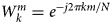 $W^{m}_k = e^{-j2 \pi k m/N}$. It is worth noting that the product of the discrete Fourier transform of x(n) and h(n) corresponds to the circular convolution of them, which in general, is not the same as the linear convolution of x(n) and h(n). However, in a special case the equality between them is held if x(n) is an OFDM signal with a cyclic prefix (CP) ≥ M 1, whereas for non-OFDM signals, the zero-padding approach can be used [Reference Haykin24].
As seen in (9), H(k) is a polynomial form of  $W^{}_k$ and is a complex coefficient (constant) representing a phase rotation and attenuation in magnitude at the frequency point k. However, H( · ) varies versus frequency in a system that is frequency-selective (including memory effects). In a linear system, the straightforward approach to determine H( · ) results from
 $H(k) = Y(k) / X(k); \, k=0, \, \ldots , \, N-1$ over the entire bandwidth of the system [Reference Oppenheim and Verghese25]. In [Reference Chiu, Zeng and Liu15], the ZF technique was used to identify the parameters of a non-linear static model in the frequency domain. However, the straightforward frequency-domain identification is not efficient in a low signal-to-noise ratio (SNR) condition and enhances the noise in the inverse modeling or ZF equalizing technique [Reference Arokiamary26]. An alternative solution is to determine H( · ) using the LS technique [Reference Kay27] within frequency sub-bands. If the bandwidths of the sub-bands are much narrower than the coherence bandwidth (B C) of the system, the sub-bands can be considered flat [Reference Molisch28] and are modeled by the zero-order polynomial in (9). Nevertheless, if the frequency response of a system cannot be considered flat within sub-bands, each sub-band is modeled by higher-orders of the polynomial in (9). In this method, multiple input and output samples contribute in the LS estimation technique, usually much more than in the straightforward approach, within each sub-band. Since a system is less frequency-selective within each sub-band compared to the entire bandwidth, the transfer function in (9) can be approximated by fewer parameters within each sub-band:
 $$ \eqalign{ \hat{H}^{\,p,q,r}_{s,\ell,u,v,w,m_2}(k) = \; & \hat{h}^{\,p,q,r}_{s,\ell,u,v,w,m_2}(0) + \hat{h}^{\,p,q,r}_{s,\ell,u,v,w,m_2}(1) \cr & \times \, W^{1}_k + \ldots + \hat{h}^{\,p,q,r}_{s,\ell,u,v,w,m_2}(O_s) \, W^{O_s}_k \cr = & \sum_{o=0}^{O_s} \hat{h}^{\,p,q,r}_{s,\ell,u,v,w,m_2}(o) \, W^{o}_k, } $$
where  $\hat {H}^{}_{s}(k)$ is an approximation of the transfer function in the sth sub-band, and O s; O s ≤ M 1 is the number of parameters.
Model identification
Time domain
Polynomial-type models are linear in parameters, hence the parameters in (6) are identified by the LS method [Reference Kay27]. The estimated parameter  $\hat { {\bf h}}_\ell $ is
 $$ \hat{{\bf h}}_\ell = ({\bf X}^H \, {\bf X})^{-1} \, {\bf X}^H \, {\bf y}_\ell, $$
where XH is the Hermitian conjugate matrix of X.
In a similar manner, the parameters of the time-domain DPD are identified using the indirect learning architecture (ILA) approach and are a copy of the parameters of the post-distorter [Reference Eun and Powers29, Reference Rönnow30]:
 $$ {\bf x}_\ell = {\bf Y} \, {\bf \theta}_\ell, $$
where xℓ is the vector of input signals, θℓ is the vector of inverse parameters, and Y is the regression matrix of output signals.
The estimated parameter  $ \hat {{\bf \theta }}_\ell $ is
 $$ \hat{{\bf \theta}}_\ell = ({\bf Y}^H \, {\bf Y})^{-1} {\bf Y}^H \, {\bf x}_\ell, $$
Frequency domain
The matrix form of (8) is given as
 $$ \eqalign{ \left( \matrix{ Y_{s,\ell}(k_0) \cr \vdots \cr Y_{s,\ell}(k_L) \cr } \right)& = \left( \matrix{ X^{0,0,0}_{s,1,1,1,0}(k_0) \, W^{0}_{k_0} & \ldots & X^{\,p,q,r}_{s,3,1,2,M_2}(k_0) \,W^{O_s}_{k_0} \cr \vdots & \vdots & \vdots \cr X^{0,0,0}_{s,1,1,1,0}(k_L) \, W^{0}_{k_L} & \ldots & X^{\,p,q,r}_{s,3,1,2,M_2}(k_L) \,W^{O_s}_{k_L}} \right)\cr & \quad \ \left( \matrix{ \hat{h}^{0,0,0}_{s,\ell,1,1,1,0}(0) \cr \vdots \cr \hat{h}^{\,p,q,r}_{s,\ell,3,1,2,M_2}(O_s) \cr } \right),} $$
where  $k_0, \ldots , k_L;\, L = N/N_S-1$ (N is the number of DFT points and N S is the number of sub-bands) are indexes of DFT in the sth sub-band, and Y s,ℓ is the frequency-domain output of the ℓth channel in the sth sub-band. The LS method is used to identify the parameters of the frequency-domain model in (14) in each frequency sub-band.
For a narrow sub-band O s ≤ M 1 and L ≤ N, hence the size of the model in (14) is smaller than in (6). The bandwidth of sub-bands is chosen due to the frequency selectivity of a system for achieving the best model performance in terms of NMSE, ACEPR, and ACLR criteria. The optimum bandwidth of sub-bands might be different for each criterion, since the NMSE criterion mostly refers to the in-band error, to which the fundamental and lower-order components make major contributions, whereas the ACEPR and ACLR criteria refer to the out-of-band errors, which only non-linear components are contributing and have less frequency selectivity.
The number of DFT points can be interpreted as the number of samples within each frequency sub-bands. If the number of DFT points increases, more samples in frequency domain are incorporated in the LS method to estimate the parameters for each sub-band. Therefore, the error will decrease as long as increasing the number of DFT points provides more information of statistical properties of the signal in the frequency domain. However, the bandwidth of sub-bands mostly depends on the frequency selectivity of the system, but not explicitly on the number of DFT points. Hence, the number of parameters for each sub-band will not directly change by increasing or decreasing the number of DFT points.
Evaluation metrics
The NMSE, ACEPR, and ACLR criteria were used to evaluate the performance of time- and frequency-domain models and DPD techniques. The NMSE [Reference Ghannouchi, Hammi and Helaoui1] of a 3D model is averaged and given as
 $$ {\rm NMSE} = {{1} \over {3}}\sum_{\ell=1}^{3} {{\sum_{n}^{} \vert y_{e,\ell}(n)\vert ^2 } \over {\sum_{n}^{} \vert y_{d,\ell}(n) \vert ^2}} , $$
where the numerator is the power of the output error and the denominator is the power of the desired output signal.
The ACEPR [Reference Isaksson, Wisell and Händel31] of a 3D model is defined as
 $$ \eqalign{ {\rm ACEPR} = {{1} \over {3}} \sum_{\ell=1}^{3} {{\int_{ {\rm adj. ch.}} \Phi_{e,\ell}(\,f) \, {\rm d}f \, } \over {\int_{{\rm ch.}} \Phi_{d,\ell}(\,f) \, {\rm d}f}}, } $$
where Φe,ℓ(f) is the power spectral density (PSD) of the model errors over the adjacent channels, Φd,ℓ(f) is the PSD of the desired output signal over the signal channel. The ACEPR is suitable for evaluating the performance of behavioral models.
The ACLR [Reference Ghannouchi, Hammi and Helaoui1] of a 3D model is
 $$ \eqalign{ {\rm ACLR} = {{1} \over {3}}\sum_{\ell=1}^{3} {{\int_{ {\rm adj. ch.}} \Phi_{y,\ell}(\,f) \, {\rm d}f \, } \over {\int_{{\rm ch.}} \Phi_{d,\ell}(\,f) \, {\rm d}f}}, } $$
where Φy,ℓ(f) is the PSD of the output signal over the adjacent channels. The ACLR is often used for evaluating the performance in DPD applications.
Experimental setup
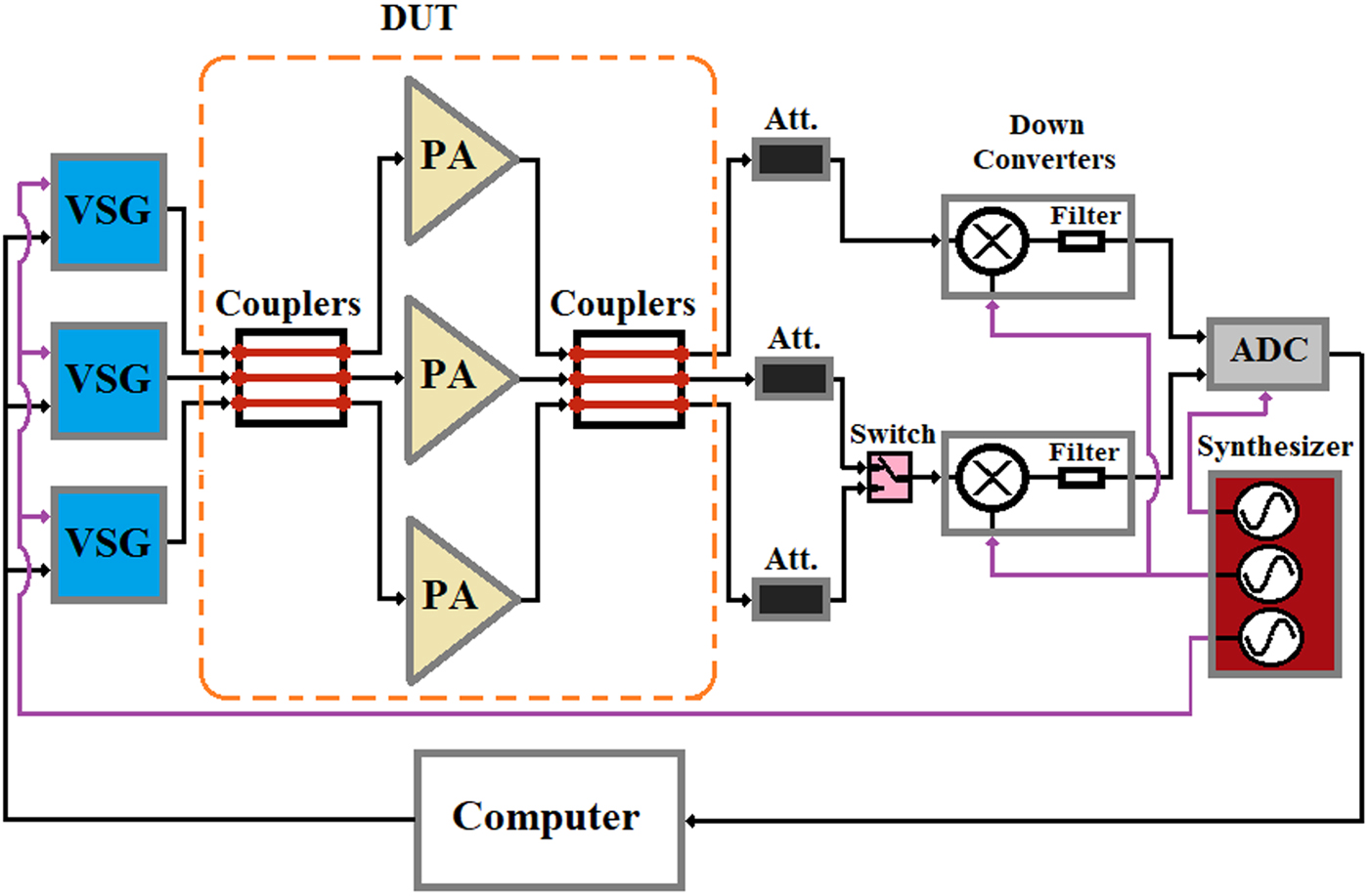
The experimental setup is shown in Fig. 2. The baseband signals were uploaded to three Rohde & Schwarz SMBV100A vector signal generators (VSGs). The maximum RF bandwidth of the VSGs is 120 MHz. The VSGs are synchronized in a 10 MHz reference clock, digital baseband clock, and LO clock. The device-under-test (DUT) consisted of three Mini-Circuits ZHL-42 RF amplifiers, which are classified as medium-high PAs, with nominal linear gains of 31.5 dB and 1-dB compression points at outputs of 30 dBm. Two types of couplers were used to resemble the cross-talk effects at the inputs and outputs in a 3 × 3 MIMO system. The couplers were 50 Ω microstrip transmission line fabricated on FR4 substrate. For the first type of couplers, the couplings between the outer and inner channels were measured using a vector network analyzer (VNA) to be − 13.5 dB, and between the two outer channels were − 21.5 dB: they are termed as “(− 13.5, − 21.5)-dB” type of couplers. The second type of couplers have − 20 dB couplings between two adjacent channels and − 35 dB between two outer channels: they are termed as “(− 20, − 35)-dB” type couplers. Three 40 dB attenuators were used to protect the components in the next stages and also to minimize the non-linear effects of the mixers.
The experimental setup.
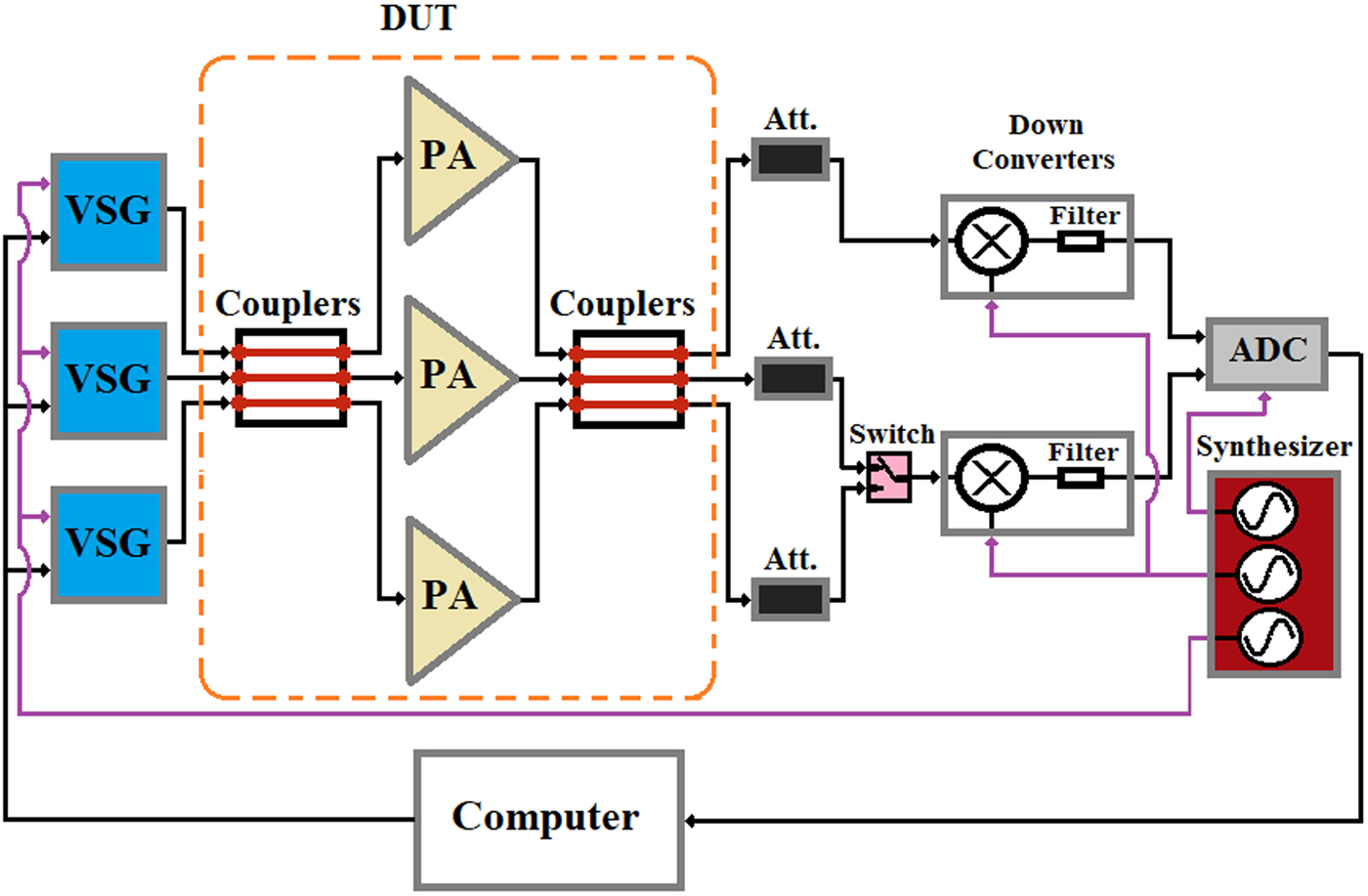
The identification and validation were done in the baseband region. The complex baseband signals were OFDM signals with 30 MHz bandwidth including 512 sub-carriers and the length of CP was 32. The baseband signals were sampled at 100 MHz and up-converted to the carrier frequency f c = 2.14 GHz with the average power of − 7.5 dBm and PAPR ~ 7.5 dB, which the excitation signals drive the amplifiers into above their 1-dB compression points. The output RF signals were down-converted to an intermediate frequency (IF) using mixers, Mini-Circuits ZX05-42MH-S, and thereafter filtered by bandpass filters. The IF signals were digitized by an analogue-to-digital converter (ADC) 14-bit SP-Device ADQ214 at a 400 MHz sampling rate. An RF coaxial switch was used to capture the signals of the three outputs by the dual-channel ADC. The insertion loss of the switch is < 0.1 dB in the frequency range DC - 4 GHz. The digitized IF signals were converted to the complex baseband region in the post-processing part. To improve the performance of the measurement system, 100 coherent averages were performed and then time-aligned with the input signal [Reference Isaksson, Wisell and Rönnow32]. An RF synthesizer Holzworth HS9003A was used to cohere the phases between the VSG, down-converter and ADC.
Results
In this section, the performances of the proposed techniques in the time and frequency domains are analyzed in a 3 × 3 MIMO system including input and output cross-talks. The first analyses are for the behavioral models, and the second for the DPD techniques. The performances are evaluated by the standard metrics NMSE, ACEPR, ACLR, and by the error spectrum. The order of non-linearity of the models is chosen as 7 due to the performances of the models. The proposed models have been tested for the available RF PAs. The amplifiers only show major dynamic behaviors along diagonal terms using MP-type models, whereas the memory effects along cross-terms are not significant [Reference Alizadeh, Rönnow, Händel and Isaksson13]. Thus, the models used for both behavioral modeling and DPD techniques are based on the MP model where M 2 = 0 in (4) and (8).
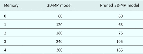
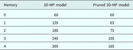
The higher-order Volterra kernels of a PA show fewer memory effects than the fundamental and lower-order kernels [Reference Zhu, Dooley and Brazil33]. Therefore, a basic pruning technique is applied to reduce the number of parameters of the model in the time domain by incorporating fewer memory samples for modeling the higher-order kernels. This approach is referred to as a non-uniform memory polynomial model [Reference Ghannouchi, Hammi and Helaoui1]. The same approach is also applied for the model in the frequency domain. Table 1 shows the number of parameters of the models without and with pruning with respect to the different memory samples.
The number of parameters versus memory length for the 3D MP time-domain model and pruned model in a 3 × 3 MIMO systems. The maximum order of the models is 7.
Behavioral model
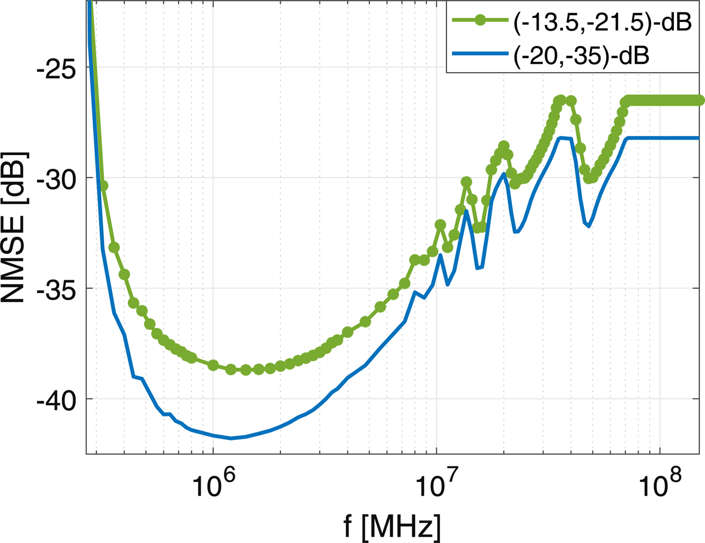
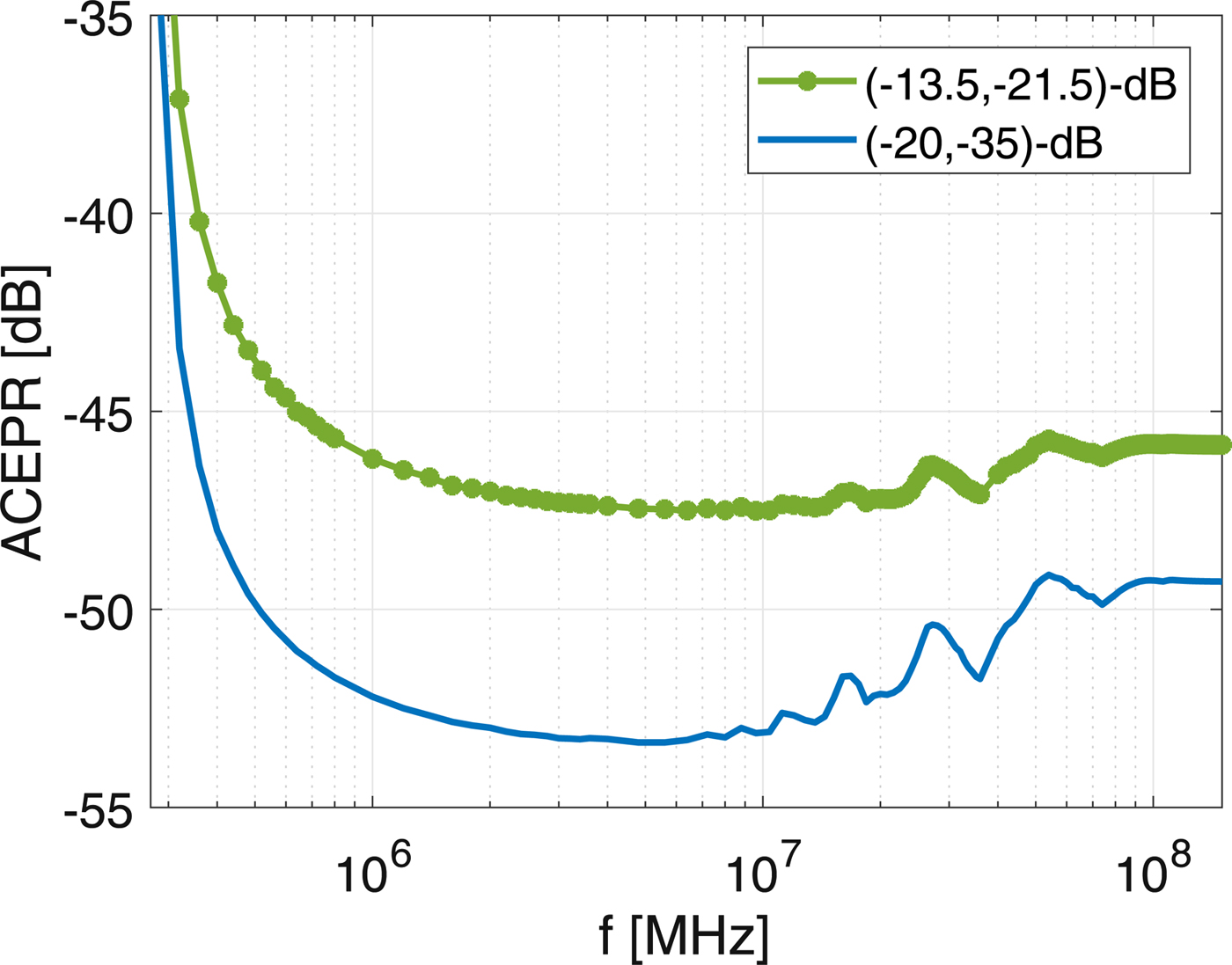
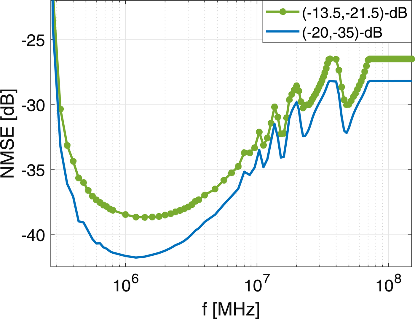
Figure 3 depicts the performance of the frequency-domain model in terms of NMSE versus the bandwidth of the sub-bands. The parameters of the model are estimated by the zero-order polynomial in (10). The best performance in NMSE is achieved when the bandwidth of the sub-bands is ~ 1.4 MHz and 1.2 MHz for (− 13.5, − 21.5)-dB and (− 20, − 35)-dB cross-talks, respectively, but the performance degrades dramatically with distances from the optimal bandwidth of the sub-bands, denoting that the system is frequency-selective for fundamental components. The curve corresponding to the (− 13.5, − 21.5)-dB type of cross-talks is smoother and less frequency-selective near the optimal bandwidth of sub-bands than the (− 20, − 35)-dB type of cross-talks. The behavior of the PAs in terms of ACEPR is different from that in NMSE, as shown in Fig. 4. The performance in ACEPR versus the bandwidth of the sub-bands is smoother (< 0.2 dB) for a wide range (~ 9 MHz), indicating that the system is not significantly frequency-selective for non-linear components.
The performance in terms of NMSE versus the bandwidth of sub-bands for the frequency-domain model estimated by the zero-order (O s = 0) polynomial in (10). The system was tested in two scenarios using two different couplers: (− 13.5, − 21.5)-dB and (− 20, − 35)-dB types of cross-talks.
The performance in terms of ACEPR versus the bandwidth of sub-bands for the frequency-domain model estimated by the zero-order (O s = 0) polynomial in (10). The system was tested in two scenarios using two different couplers: (− 13.5, − 21.5)-dB and (− 20, − 35)-dB types of cross-talks.
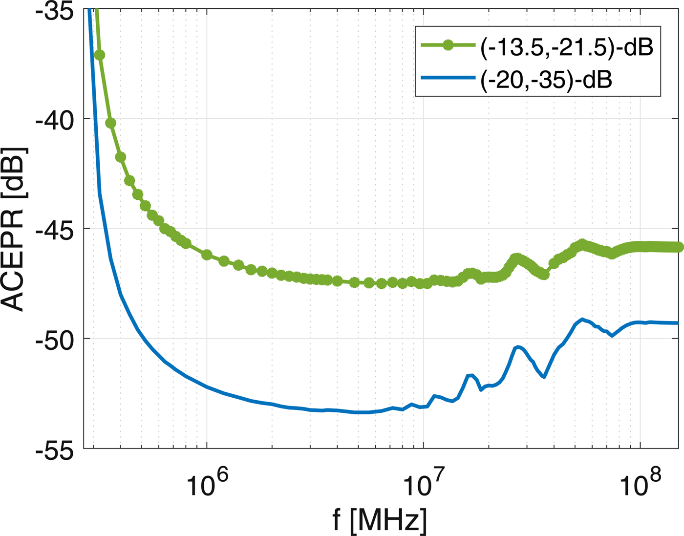
The optimal bandwidth of the sub-bands depends on the frequency selectivity of a system due to the bandwidth of the excitation signal. On the one hand, by increasing the bandwidth of the sub-bands, the number of DFT points incorporating into the parameters estimation increases in (14), and hence the model error decreases. On the other hand, sub-bands with wider bandwidths are more frequency-selective, and hence the model error increases. Therefore, there is a trade-off between the bandwidth of the sub-bands and the number of samples for LS estimation (for a fixed number of DFT points N).
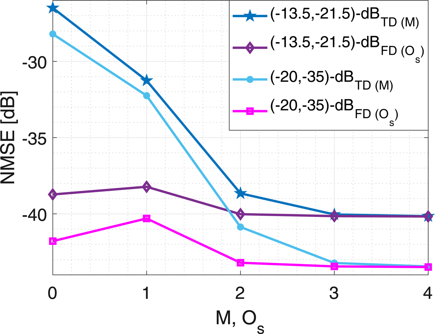
The performances of both the time- and frequency-domain models in terms of NMSE are depicted in Fig. 5. The NMSE in the time-domain modeling shows that the system is dynamic in the in-band frequency region; the model detects three memories of the system. The performance of the frequency-domain model estimated by the zero-order of polynomial in (10) gives more than 12 dB gain compared to the memory-less time-domain model. However, the performance of the frequency-domain model estimated by the second-order polynomial will improve by ~ 1 dB, which implies that the sub-bands are slightly frequency-selective.
The performances in terms of NMSE for the time-domain (TD) and frequency-domain (FD) models versus the memory length (M) and order of polynomial (O s) in (10), respectively. The bandwidths of sub-bands are 1.4 and 1.2 MHz for (− 13.5, − 21.5)-dB and (− 20, − 35)-dB types of cross-talks, respectively.
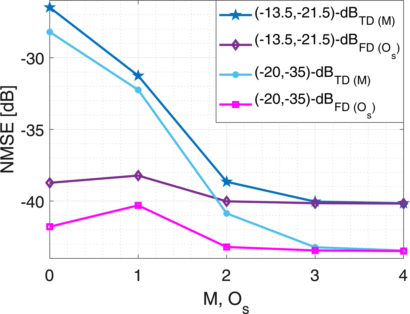
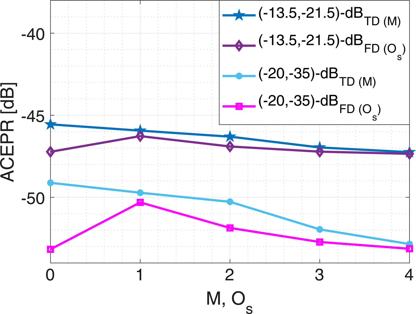
Figure 6 illustrates the performance of both models in terms of ACEPR. The time-domain model detects three memories of the dynamic system, but the memory effect is less significant compared to what the NMSE criterion detects, meaning the system is less dispersive in non-linear components. The performance of the frequency-domain model shows that each sub-band could be estimated by the zero-order polynomial model in (10), which indicates that the sub-bands are not frequency-selective for non-linear components. These are consistent with the analyses of the NMSE and ACEPR versus the bandwidth of the sub-bands as shown in Figs 3 and 4.
The performance in terms of ACEPR for the time-domain (TD) and frequency-domain (FD) models versus the memory length (M) and order of polynomial (O s) in (10), respectively. The bandwidths of sub-bands are 6.4 and 4.8 MHz for (− 13.5, − 21.5)-dB and (− 20, − 35)-dB types of cross-talks, respectively.
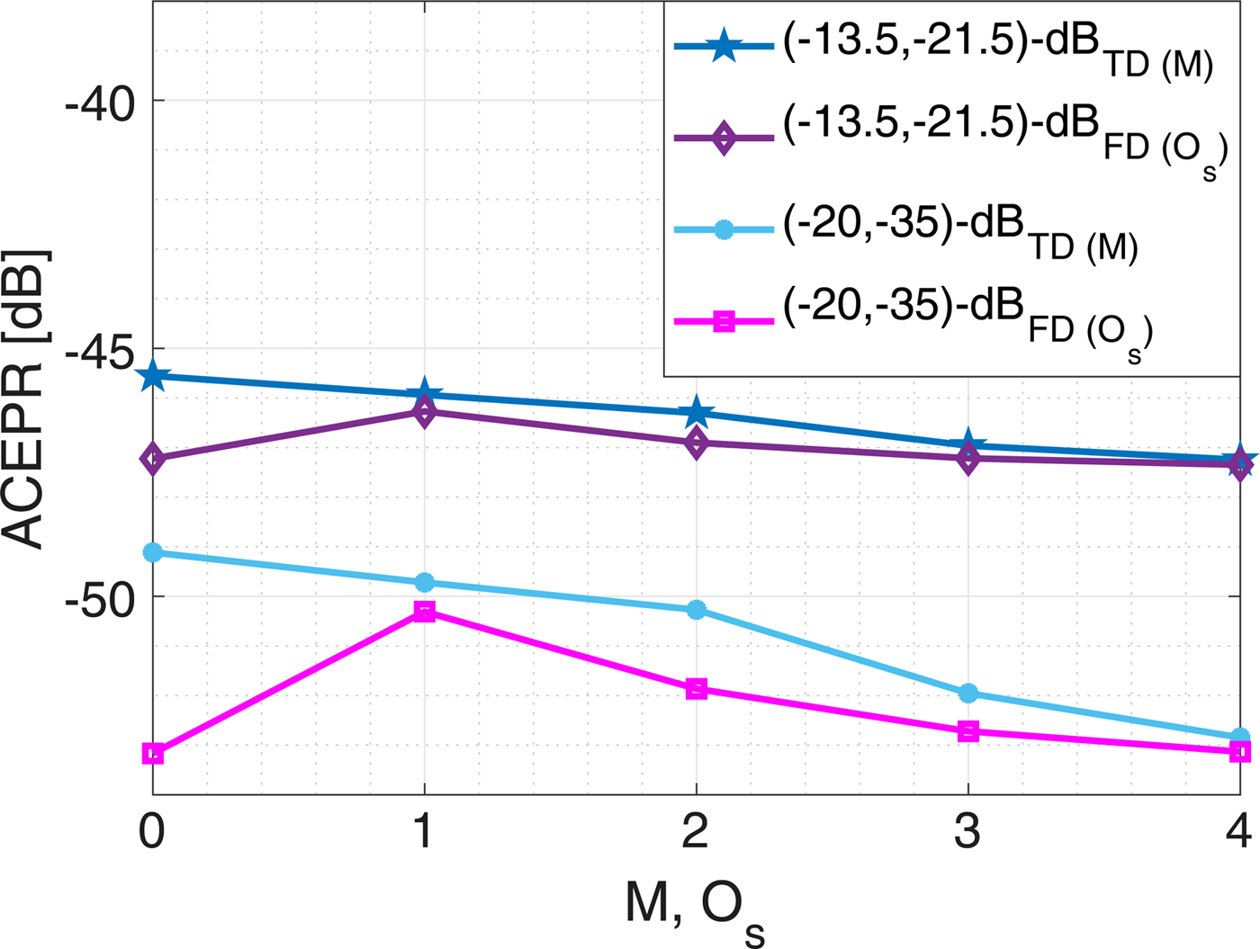
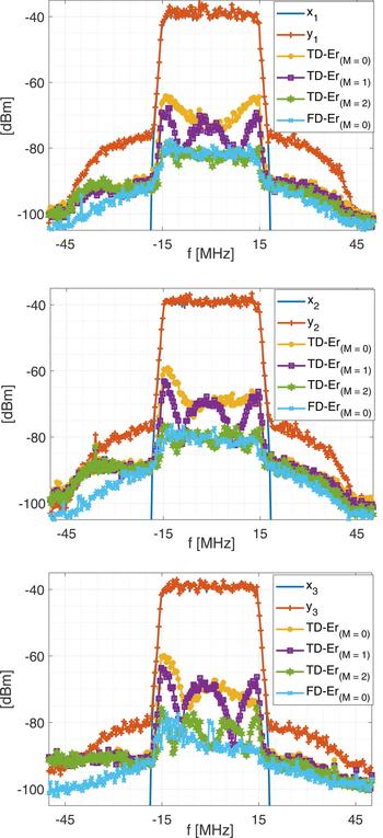
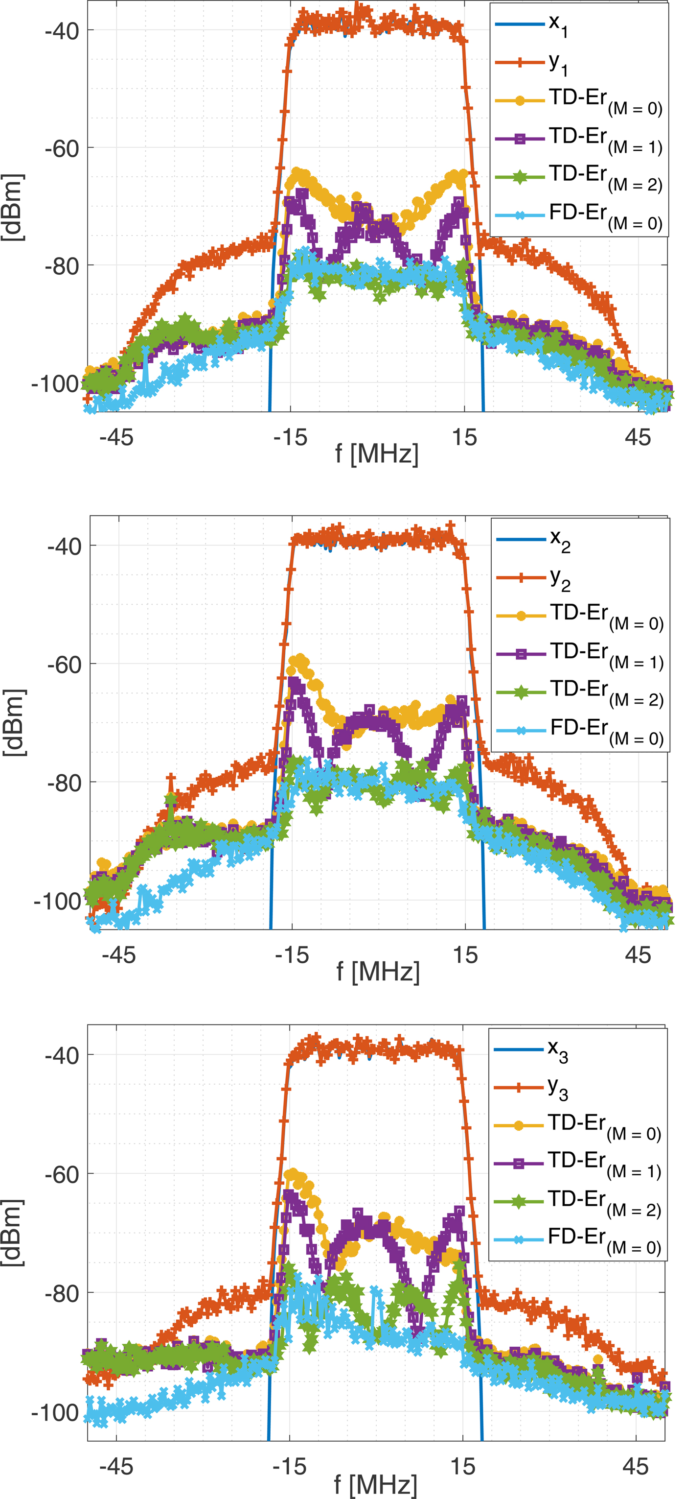
Figure 7 depicts the PSD of the input and output signals of the PAs, the spectrum of the errors of the time-domain model for M = 0, 1, 2 and of the frequency-domain model for O s = 0 in a 3 × 3 MIMO system. As expected, the frequency-domain model (O s = 0) outperforms the time-domain model in both NMSE and ACEPR for M<2. This superiority is more significant in NMSE than ACEPR, since the system is less frequency-selective in the out-of-band frequency regions.
The PSD of the input and outputs of the DUT, the error spectrum of the time-domain model (TD-Er) for M = 0, 1, 2 and the frequency-domain model (FD-Er) for O s = 0. x ℓ and y ℓ are the ℓth input and output signals in a 3 × 3 MIMO system. The type of cross-talk (− 20, − 35)-dB was used. The bandwidths of sub-bands are 1.2 and 4.8 MHz for estimating the parameters within the input signal channel and adjacent channels.
Digital pre-distortion
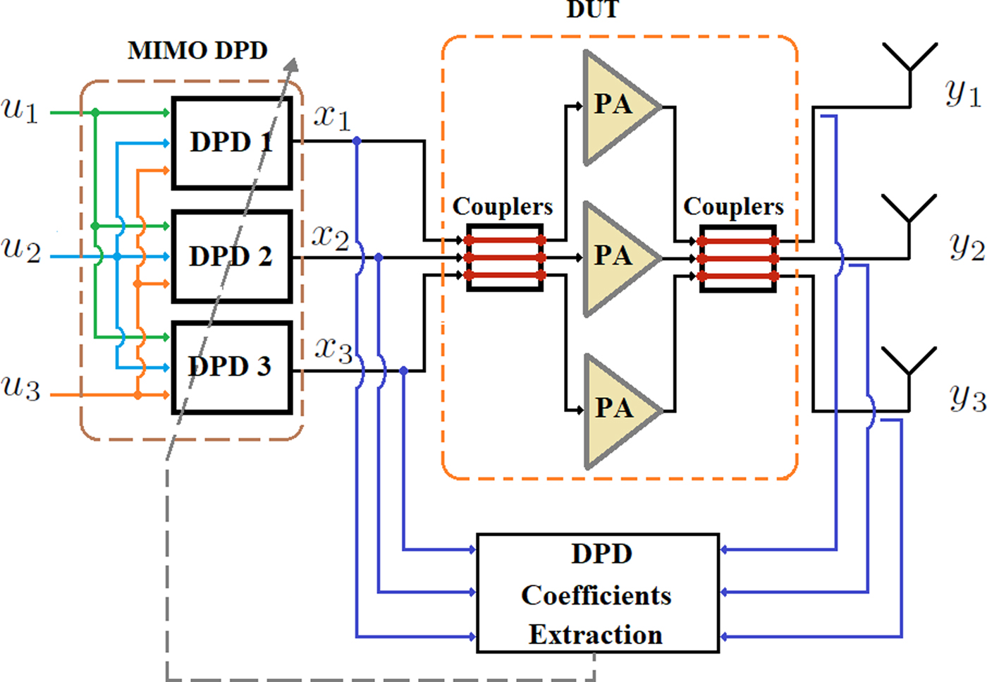
The 3D time- and frequency-domain pre-distortion techniques are proposed in ILA architecture to compensate the impairments of the DUT by considering two assumptions: first, the impairments of the in-phase and quadrature (IQ) imbalances in VSGs are minor and negligible; second, the non-linearity and memory effects of the VSGs are included in those of the DUT. An MP-type model is chosen for the DPD technique, since the GMP model does not detect the memory effect of the DUT along cross-terms [Reference Alizadeh, Rönnow, Händel and Isaksson13]. The block diagram of the 3D digital pre-distorter is shown in Fig. 8.
The block diagram of the 3D DPD structure.

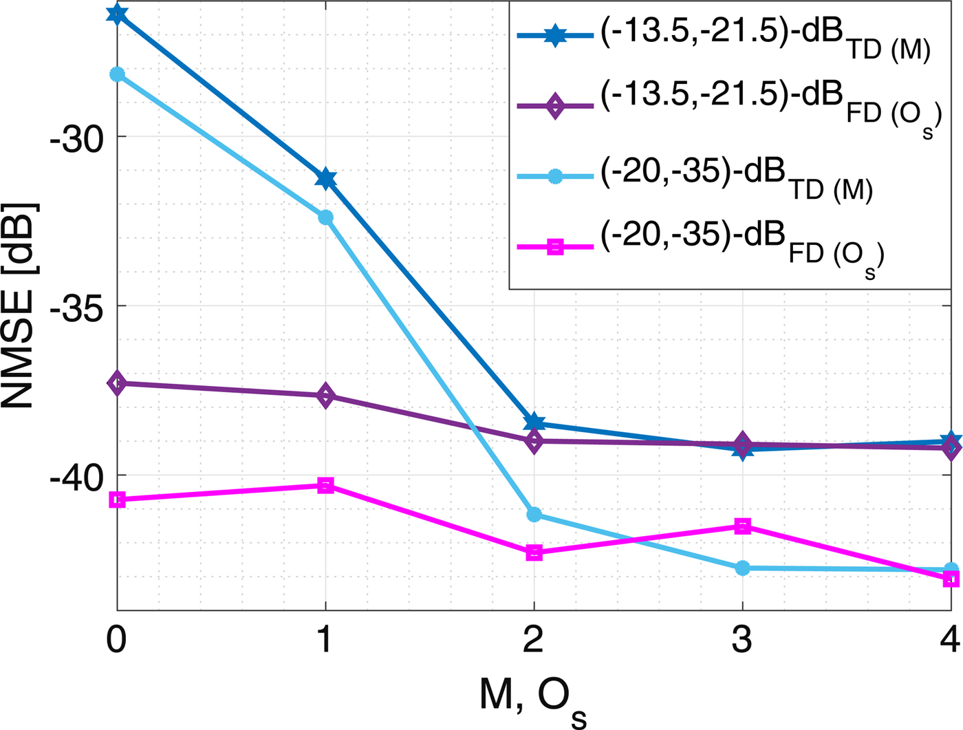
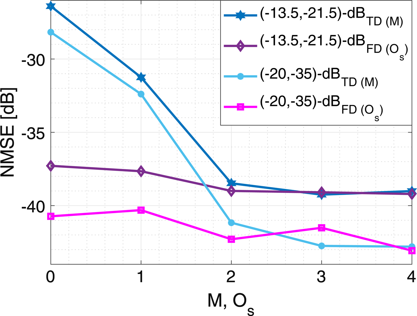
The performance of the 3D DPD in terms of NMSE is depicted in Fig. 9. The time-domain DPD detects three memory samples of the system, which is the same as in the modeling. Nevertheless, the memory effects in the DPD are less pronounced than in the modeling (cf. Fig. 5). The NMSEs of the signals without using DPD technique are − 11.25 and − 13.17 dB for the (− 13.5, − 21.5)-dB and (− 20, − 35)-dB types of cross-talks, respectively. However, the NMSEs after using 3D DPD improve by ~ 27.5 and ~ 29.6 dB for M=2, whereas three SISO DPDs improve the NMSEs by 2.81 and 0.49 dB for the (− 13.5, − 21.5)-dB and (− 20, − 35)-dB types of cross-talks, respectively. The performance of the frequency-domain 3D DPD estimated by the zero-order polynomial in (10) outperforms the memory-less time-domain's by ~ 9.9 dB in terms of NMSE. However, the sub-bands are slightly frequency-selective, as is modeled by the second-order polynomial in (10), giving about 1 dB improvement.
The performances in terms of NMSE for the time-domain (TD) and frequency-domain (FD) DPDs versus the memory length (M) and order of polynomial (O s) in (10), respectively. The NMSE without DPDs are − 11.25 and − 13.17 dB in the case of (− 13.5, − 21.5)-dB and (− 20, − 35)-dB types of cross-talks, respectively.
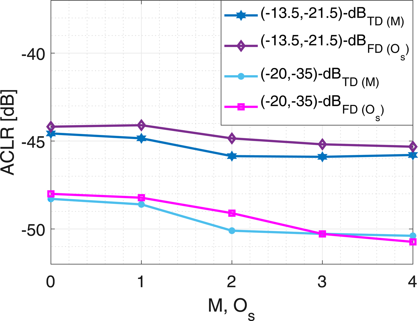
The performance of the DPDs in terms of ACLR is shown in Fig. 10, whereas the ACLRs without DPD are − 38.85 and − 39.82 dB. Three SISO DPDs improve the ACLRs by 3 and 3.33 dB for the (− 13.5, − 21.5)-dB and and (− 20, − 35)-dB types of cross-talks, respectively. The time- and frequency-domain DPDs merely detect the static behavior of the system. Hence, both techniques approximately give the same performance in ACLR.
The performances in terms of ACLR for the time-domain (TD) and frequency-domain (FD) DPDs versus the memory length (M) and order of polynomial (O s) in (10), respectively. The NMSE without DPDs are − 38.85 and − 39.82 dB in the case of (− 13.5, − 21.5)-dB and (− 20, − 35)-dB types of cross-talks, respectively.
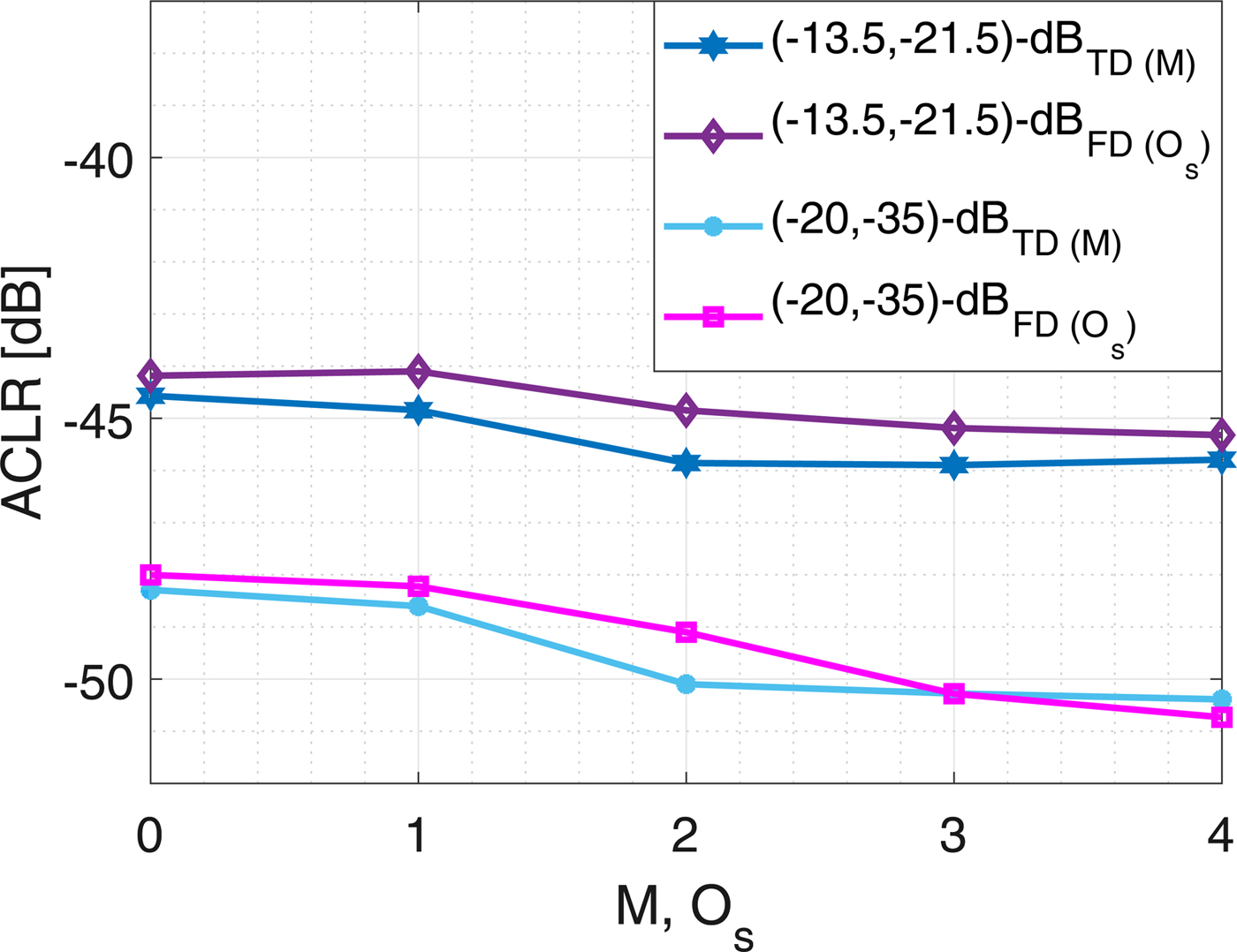
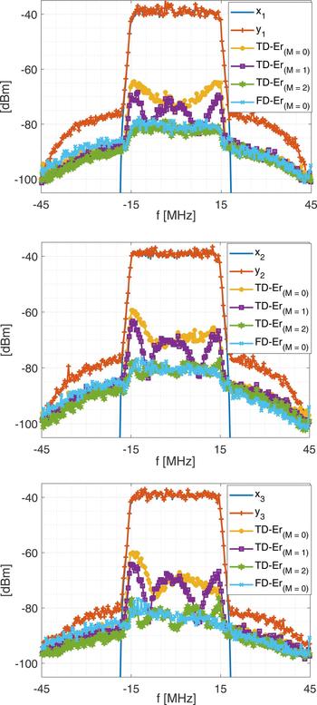
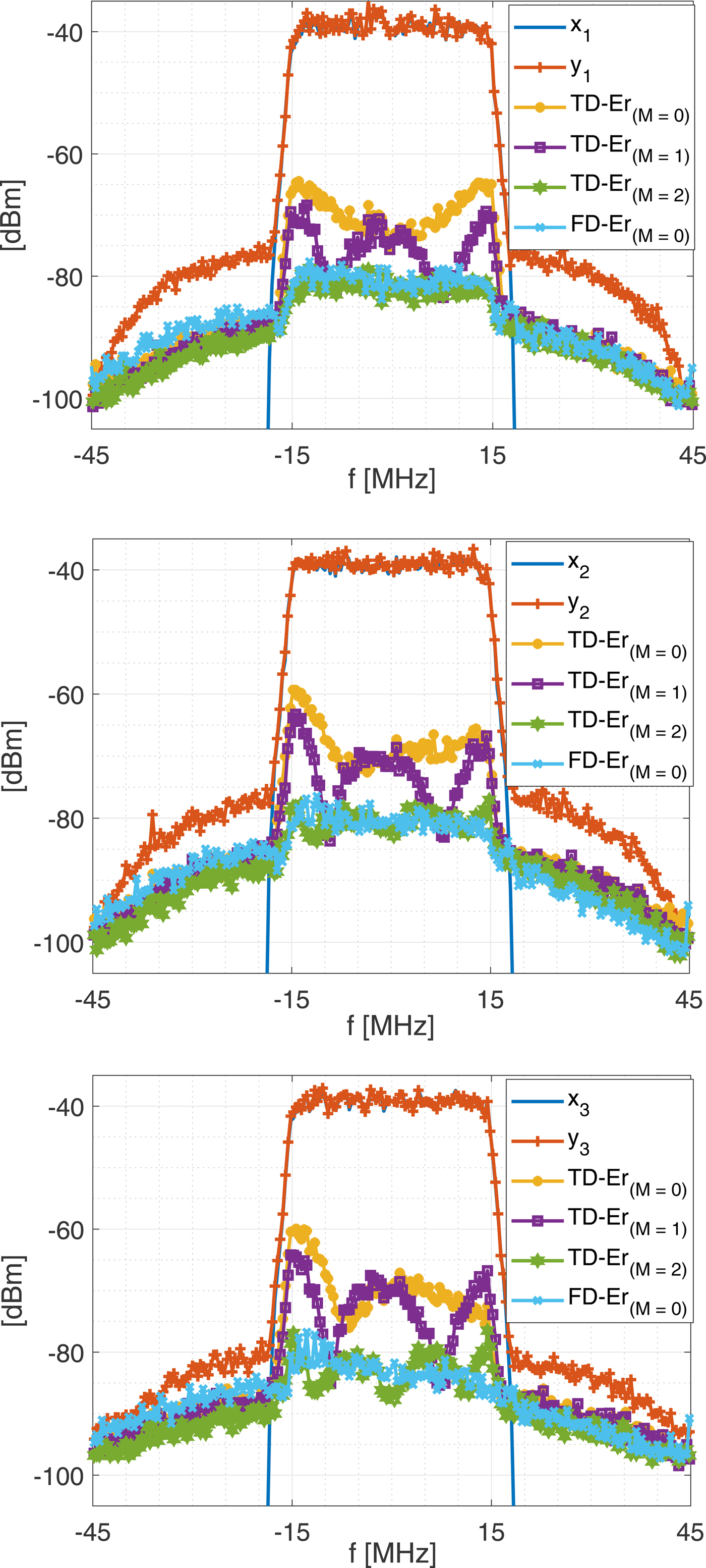
Figure 11 illustrates the PSD of the input and output signals of the PAs, the spectrum of the errors of the time-domain DPD for M = 0, 1, 2 and of the frequency-domain DPD for O s = 0 in a 3 × 3 MIMO system. As shown, the frequency-domain DPD (O s = 0) outperforms the time-domain model in NMSE for M < 2.
The PSD of the input and outputs of the DUT, the error spectrum of the time-domain DPD (TD-Er) for M = 0, 1, 2 and the frequency-domain DPD (FD-Er) for O s = 0. x ℓ and y ℓ are the ℓth input and output signals in a 3 × 3 MIMO system. The type of cross-talk (− 20, − 35)-dB was used.
Computational complexity
The size of the regression matrix for a time-domain MP model is
 $$ N \, K_0 \, (1 + M), $$
where N is the number of samples, M is the memory length, and K 0 is the total number of parameters in a static model, which is 60 for P = 7 in a 3 × 3 MIMO system. The computational complexity of the parameter estimation in (11) using a Gaussian elimination method [Reference Strang34] is
 $$ \eqalign{ & 3 N K_0 \, (1+M) + 2 N K^{2}_0 \, (1+M)^2 \cr & \quad + K^{3}_0 \, (1+ M)^3 ,} $$
where only the computational complexity of multiplications is considered [Reference Guan and Zhu35], since the number of floating points operations (FLOPs) for a complex multiplication is 6, whereas for a complex addition it is 2 [Reference Tehrani, Haiying, Afsardoost, Eriksson, Isaksson and Fager36]. If the entire bandwidth of the system is divided into N s sub-bands, the size of the regression matrix in a sub-model is
 $$ {{N} \over {N_s}} \, K_0 \, (1+O_s). $$
The total computational complexity of the parameter estimation for all sub-models, including the fast Fourier transform (FFT) and inverse fast Fourier transform (IFFT), is
 $$ \eqalign{ K_0 \, & N \, {\rm log}_2 (N) + 3 N \, {\rm log}_2 (N) + 3 N K_0 (1+O_s) \cr & + 2 N K^{2}_0 (1+O_s)^2 + N_s K^{3}_0 (1+O_s)^3 \cr & \quad + N K_0 O_s. } $$
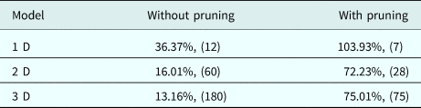
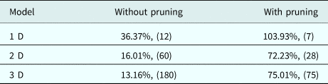
A sub-band is much narrower than the entire bandwidth of the system, O s ≤ M. Also, the size of the frequency-domain sub-model in (20) is smaller than the time-domain model in (18) by a factor of (1 + O s)/(N s (1 + M)). Therefore, the total computational complexity of the sub-band modelling in the frequency domain is less than the time-domain's. Table 2 shows the relative computational complexity of the frequency-domain technique compared to the time-domain technique for 1D, 2D, and 3D techniques where it is assumed that MP models are used, M = 2, O s = 0, N s = 38, N = 25 000, and P=7 in all cases. As shown, the computational efficiency of the frequency-domain technique is low for small size of models. However, its efficiency increases for models with large number of parameters, e.g. for the 3D model: the computational complexity of the frequency-domain model reduces by ~ 87% and 25% compared to the time-domain model's in the case of without (180 parameters) and with pruning (75 parameters), respectively
The relative computational complexity of the frequency-domain technique compared to the time-domain technique for 1D, 2D, and 3D techniques where it is assumed that MP models are used, M = 2, O s = 0, N s = 38, N = 25 000 and P = 7 in all cases. The number of parameters of the time-domain model for each case is mentioned in the parenthesis.
In addition, the frequency-domain parameters identification can be done independently for each sub-band, which is an advantage for parallel processing applications. Furthermore, the frequency-domain approach is more feasible for economic processors and embedded systems.
Discussion
The method presented above, where analytical expressions in the frequency domain are fitted to experimental data and then transformed to the time domain, does not enforce causality of the final time-domain model. If the bandwidth of the frequency-domain sub-band model is narrower than the bandwidth of a DUT or excitation signals, the output of the model could be noticeably affected by the non-causality of the model. Also, these effects happen for the excitation signals with abrupt changes, e.g. impulse-like signals, which it is necessary to filter. Thus, the model shows some non-causality effects in cases of narrow sub-band bandwidths, low SNR, a high maximum order of non-linearity and limited memory length of the DUT. In some applications in which DUTs are excited by burst signals, the effects of non-causality might be a concern. However, these effects are negligible if they are below the noise level. Nonetheless, the proposed frequency-domain sub-band modeling technique processes a (non-burst) sequence or block of time-domain data transformed in the frequency domain. Hence, the effects of non-causal processing can be neglected for a sequence that can be considered as an off-line data.
In this paper, the behavioral modeling and DPD methods are investigated for RF PAs under output impedance matched conditions, for which it is assumed that the effects of non-linearity caused by reflected signals from antennas are negligible. Otherwise, the model requires different strategies to tackle the problem [Reference Hausmair, Landin, Gustavsson, Fager and Eriksson14]. However, the linear effects of the output cross-talk are considered in this work. Besides that, the structure of the proposed DPD model is suitable to compensate for the effects of both input and output cross-talk channels. Nevertheless, it might be modified for other types of cross-talks, e.g. if the DUT only includes input (or output) cross-talk channels [Reference Amin, Landin, Händel and Rönnow10, Reference Rönnow30]. The method for the proposed frequency-domain modelling technique in this paper would be suitable for gallium nitride (GaN) RF PAs and millimetre-wave applications, in which it is required to include long-term memory effects in time-domain modeling techniques [Reference Barradas, Cunha and Pedro37, Reference Amin, Händel and Rönnow38].
Conclusion
In this paper, 3D behavioral models and DPD techniques are proposed in both the time and frequency domains for RF PAs in a 3 × 3 MIMO system including input and output cross-talks. The performances of the proposed techniques in both domains are evaluated giving improvements in minimizing the errors in terms of NMSE, ACEPR, and ACLR. The proposed frequency-domain technique has the advantage of reducing the computational complexity, which makes it suitable for higher-dimensional MIMO systems, and also for strong dynamic systems. Moreover, the frequency-domain technique has a higher efficiency compared to the time-domain technique for a system that is dispersive along diagonal terms. Hence, future research can be focused on the extension of the work for massive MIMO and millimetre-wave systems.
Author ORCIDs
Mahmoud Alizadeh, 0000-0003-2061-6366
 Mahmoud Alizadeh received the M.Sc. degree in wireless communication from the Electrical and Information Technology Department, Lund University, Lund, Sweden, in 2013, and received the Ph.D. degree with the School of Electrical Engineering and Computer Science, Royal Institute of Technology (KTH), Stockholm, Sweden in 2019, focusing on digital signal processing for communication systems, linearisation and characterisation techniques for non-linear RF power amplifiers. He was also with the Department of Electronical Engineering, Mathematics and Natural Sciences, University of Gävle, Gävle, Sweden.
 Peter Händel received the M.Sc. degree in Engineering Physics and Ph.D. degree in Automatic Control from the Department of Information Technology, Uppsala University, Uppsala, Sweden, in 1987 and 1993, respectively. During 1993–1997, he was with the Research and Development Division, Ericsson Radio Systems AB, Kista, Sweden. Since August 1997, he has been in the School of Electrical Engineering and Computer Science, Royal Institute of Technology (KTH), Stockholm, Sweden, where he currently is Professor of the Division of Information Science and Engineering.
 Daniel Rönnow received the M.Sc. degree in Engineering Physics and Ph.D. degree in Solid-state Physics from Uppsala University, Uppsala, Sweden, in 1991 and 1996, respectively. He was involved with semiconductor physics at Max-Planck-Institut für Festkörperforschung, Stuttgart, Germany, from 1996 to 1998 and with infrared sensors and systems at Acreo AB, Stockholm, Sweden, from 1998 to 2000. From 2000 to 2004, he was a Technical Consultant and Head of Research with Racomna AB, Uppsala, Sweden. From 2004 to 2006 he was a university lecturer at University of Gävle, Sweden. During 2006–2011 he was a senior sensor engineer at Westerngeco, Oslo Norway, where he worked with signal processing and seismic sensors. In 2011, he became a professor in electronics at University of Gävle. He has been an Associate Professor with Uppsala University since 2000. He has authored or coauthored over 45 peer-reviewed papers and holds eight patents. His current research interests are RF measurement techniques, and linearization of non-linear RF circuits and systems.