1 Introduction
Two-dimensional turbulence is fundamentally important to geophysical and astrophysical fluid dynamics. Large-scale planetary and astrophysical flows are frequently quasi-two-dimensional, with vertical motions constrained by aspect ratio, stratification and rotation. In such flows, the dual conservation of kinetic energy and enstrophy causes enstrophy to move to small scales while energy moves to large scales in the celebrated inverse energy cascade, one of the most remarkable features of all fluid dynamics.
A major outstanding problem in two-dimensional turbulence is the degree to which the inverse energy cascade is quasi-Gaussian and exhibits an energy spectrum satisfying
 $E(k)\sim k^{-5/3}$
, as predicted by Kraichnan (Reference Kraichnan1967). Forcing the flow at strongly dissipated small scales suppresses nonlinear interactions and inhibits the enstrophy cascade (Smith & Yakhot Reference Smith and Yakhot1993), resulting in relatively featureless vorticity fields and inverse cascades with
 $k^{-5/3}$
spectra, as found in a number of studies (Frisch & Sulem Reference Frisch and Sulem1984; Sommeria Reference Sommeria1986; Maltrud & Vallis Reference Maltrud and Vallis1991; Paret & Tabeling Reference Paret and Tabeling1998; Rutgers Reference Rutgers1998; Boffetta, Celani & Vergassola Reference Boffetta, Celani and Vergassola2000; Dubos et al.
Reference Dubos, Babiano, Paret and Tabeling2001; Bruneau & Kellay Reference Bruneau and Kellay2005; Boffetta Reference Boffetta2007). Classical theories, on the other hand, assume infinitely separated forcing and dissipation scales that allow both energy and enstrophy cascades to be present (Kraichnan Reference Kraichnan1967; Leith Reference Leith1968; Batchelor Reference Batchelor1969). To test these theories, one must force at intermediate scales sufficiently far from the dissipation range so that an enstrophy cascade can develop (Boffetta & Musacchio Reference Boffetta and Musacchio2010). In this scenario, simulated inverse cascades consistently develop populations of coherent vortices and exhibit spectra steeper than
 $k^{-5/3}$
(Smith & Yakhot Reference Smith and Yakhot1993; Borue Reference Borue1994; Scott Reference Scott2007; Vallgren Reference Vallgren2011; Fontane, Dritschel & Scott Reference Fontane, Dritschel and Scott2013; Burgess, Scott & Shepherd Reference Burgess, Scott and Shepherd2015). While coherent vortices have been characterized as spurious hypofriction effects (Boffetta & Ecke Reference Boffetta and Ecke2012) or as limited to the vicinity of the forcing scale (Boffetta et al.
Reference Boffetta, Celani and Vergassola2000), several recent studies demonstrate that vortices form under a wide range of conditions, including Laplacian diffusion and hyperviscosity, in the absence of hypodiffusion (Scott Reference Scott2007; Vallgren Reference Vallgren2011; Fontane et al.
Reference Fontane, Dritschel and Scott2013; Burgess et al.
Reference Burgess, Scott and Shepherd2015). A proper understanding of vortical features is important because the presence of such vortices in two-dimensional inverse cascades governs to a large extent the transport and mixing in quasi-two-dimensional geophysical and astrophysical flows.
Much research has been done on vortex populations in decaying two-dimensional turbulence, and several increasingly comprehensive scaling theories have been proposed. Benzi, Patarnello & Santangelo (Reference Benzi, Patarnello and Santangelo1988) and Benzi et al. (Reference Benzi, Collela, Briscolini and Santangelo1992) linked the algebraic scaling of the energy spectrum to a vortex population with an algebraic number density
 $n(A)\sim A^{-p}$
and determined
 $p$
empirically from numerical simulations. Carnevale et al. (Reference Carnevale, McWilliams, Pomeau, Weiss and Young1991) and Weiss & McWilliams (Reference Weiss and McWilliams1993) proposed a temporal scaling theory: assuming
 $N$
vortices of a single size, energy conservation and conservation of the vorticity extremum, dimensional arguments yield
 $N\sim t^{-\unicode[STIX]{x1D709}}$
, with no prediction for
 $\unicode[STIX]{x1D709}$
. Dritschel et al. (Reference Dritschel, Scott, Macaskill, Gottwald and Tran2008) proposed a theory that unified the spatial and temporal scalings of Benzi et al. (Reference Benzi, Patarnello and Santangelo1988, Reference Benzi, Collela, Briscolini and Santangelo1992), Carnevale et al. (Reference Carnevale, McWilliams, Pomeau, Weiss and Young1991) and Weiss & McWilliams (Reference Weiss and McWilliams1993) and determined the vortex number density
 $n(A)\sim t^{-2/3}A^{-1}$
using self-similarity arguments. It must be emphasized here that two-dimensional decaying turbulence and two-dimensional forced turbulence are fundamentally different systems, and there is no reason to suppose that details of the vortex population in decaying two-dimensional turbulence should have any bearing on the vortex population in forced turbulence. In fact, the very existence of a robust and well-defined vortex population in the forced inverse cascade has only recently begun to be appreciated.
In this paper we make the first attempt to develop a temporal and spatial scaling theory for the vortex population in the forced two-dimensional inverse cascade. We consider the canonical scenario of two-dimensional turbulence with a narrow-band forcing that injects kinetic energy
 $E$
and enstrophy
 $Z$
at prescribed constant rates. We demonstrate that the vortex population dominates the flow dynamics over a range of scales that increases in time. Similarity arguments and conservation considerations predict the growth rates of the largest vortex and the spectral peak length scale (§ 2), as well as the time evolution and scaling of a three-part vortex number density (§ 3). In § 4 we provide support for our predictions from high-resolution simulations.
2 Similarity theory for the forced inverse cascade
In the spirit of Batchelor’s similarity theory for decaying two-dimensional turbulence (Batchelor Reference Batchelor1969), we first construct dimensionless variables appropriate for the forced inverse cascade. Batchelor’s theory assumes that when
 $Re\rightarrow \infty$
enstrophy dissipation in decaying two-dimensional turbulence remains finite, while energy dissipation vanishes. Energy is then the only invariant, and a natural choice of similarity variable is
 $kt\sqrt{E}$
. In contrast, in the forced two-dimensional inverse cascade,
 $E$
grows at a prescribed rate while
 $Z$
must remain constant. Possible dimensionless combinations in this case are
 $$\begin{eqnarray}\displaystyle k\sqrt{4E/Z},\quad kt\sqrt{2E}, & & \displaystyle\end{eqnarray}$$
where
 $\sqrt{2E}=u_{rms}$
is the r.m.s. speed,
 $1/\sqrt{Z}$
is an eddy turnover time and we include constant factors for later convenience.
Taking
 $Z=\text{constant}$
and
 $E\sim t$
(as prescribed in our simulations), requiring
 $$\begin{eqnarray}\displaystyle k\sqrt{4E/Z}\sim 1,\quad kt\sqrt{2E}\sim 1, & & \displaystyle\end{eqnarray}$$
and associating wavenumber
 $k$
and length
 $l$
through
 $k=2\unicode[STIX]{x03C0}/l$
, we obtain two length scales and their growth rates,
 $$\begin{eqnarray}\displaystyle & \displaystyle l_{\unicode[STIX]{x1D714}}\equiv 2\sqrt{4E/Z}\sim t^{1/2}, & \displaystyle\end{eqnarray}$$
 $$\begin{eqnarray}\displaystyle & \displaystyle l_{\unicode[STIX]{x1D713}}\equiv t\sqrt{2E}\sim t^{3/2}. & \displaystyle\end{eqnarray}$$
 $l_{\unicode[STIX]{x1D714}}$
, is the characteristic length scale of the vorticity field
 $\unicode[STIX]{x1D714}$
, giving a characteristic eddy or vortex radius
 $a(t)=\sqrt{4E/Z}$
, growing as
 $t^{1/2}$
. (The factor of
 $4$
comes from relating vorticity to angular velocity.) This yields a vortex area growth rate
 $A\sim t$
, where
 $A$
is the vortex area. We identify
 $l_{\unicode[STIX]{x1D713}}$
as the relevant length scale for the streamfunction
 $\unicode[STIX]{x1D713}$
. It can be thought of as the distance travelled by a vortex moving at speed
 $u_{rms}$
in unit time.
We also define a third length scale,
 $$\begin{eqnarray}\displaystyle l_{E}=\sqrt{l_{\unicode[STIX]{x1D713}}l_{\unicode[STIX]{x1D714}}}=(2t\sqrt{8E^{2}/Z})^{1/2}\sim t, & & \displaystyle\end{eqnarray}$$
which we associate with the energy
 $E$
and an area
 $A_{eff}=l_{\unicode[STIX]{x1D714}}u_{rms}t$
, the effective area swept out in unit time by an eddy of diameter
 $l_{\unicode[STIX]{x1D714}}$
moving at speed
 $u_{rms}$
. Here
 $A_{eff}$
is the collision cross-section for vortices of area
 $A$
and is the relevant scale of interaction with the more slowly evolving streamfunction. Since
 $l_{E}$
is the characteristic scale of
 $E$
,
 $k_{E}\equiv 2\unicode[STIX]{x03C0}/l_{E}$
should roughly coincide with the spectral peak wavenumber,
 $k_{E}\approx k_{p}$
, yielding a predicted growth law
 $k_{p}\sim t^{-1}$
.
3 Vortex scaling theory
We now develop a vortex scaling theory based on material vorticity conservation and transport of conserved quantities through scaling ranges. The forcing continuously injects enstrophy, replenishing a ‘thermal bath’ of small vortices with characteristic area
 $A_{f}$
and vortex mean square vorticity at that scale
 $$\begin{eqnarray}\displaystyle \overline{\unicode[STIX]{x1D714}_{v}^{2}(A_{f})}=\frac{1}{N}\mathop{\sum }_{i=1}^{N}\frac{1}{A_{i}}\int _{A_{i}}\unicode[STIX]{x1D714}^{2}\,\text{d}^{2}x, & & \displaystyle\end{eqnarray}$$
where
 $N$
is the total number of such vortices, and
 $A_{i}\approx A_{f}$
, i.e. the vortices start with approximately the same size, which is set by the forcing. The mean square vorticity
 $\overline{\unicode[STIX]{x1D714}_{v}^{2}(A)}$
of vortices with arbitrary area
 $A$
is similarly defined. Vortices nucleated at the forcing scale grow by merging with other like-sign vortices. Since
 $\overline{\unicode[STIX]{x1D714}_{v}^{2}(A_{f})}$
is set by the forcing, and since merger cannot change the vorticity of fluid parcels, but only aggregate them into larger structures, it is reasonable to assume that
 $\overline{\unicode[STIX]{x1D714}_{v}^{2}(A_{f})}=\overline{\unicode[STIX]{x1D714}_{v}^{2}(A)}$
, i.e.
 $\overline{\unicode[STIX]{x1D714}_{v}^{2}}$
is independent of
 $A$
. Since the system is continuously forced, we leave open the possibility that
 $\overline{\unicode[STIX]{x1D714}_{v}^{2}}$
may grow in time.
We expect the forcing to replace enstrophy lost to filament shedding during merger such that the total area fraction occupied by coherent vortices,
 $$\begin{eqnarray}\displaystyle f_{v}=\frac{1}{{\mathcal{D}}}\int _{A_{f}}^{A_{max}}An(A)\,\text{d}A, & & \displaystyle\end{eqnarray}$$
is constant, where
 $n(A)$
is the vortex number density,
 ${\mathcal{D}}$
is the area of the domain and
 $A_{max}$
is the area of the largest vortex. This prediction is well supported by our numerical simulations, as discussed below. In terms of vortex dynamics, enstrophy is protected within large-scale coherent structures and only lost to the enstrophy cascade through filamentation during mergers. Loss of coherent enstrophy through a succession of merger and filamentation events frees up a region, which a newly nucleated vortex will occupy.
Systems far from equilibrium can exhibit multiple regimes with distinct scaling behaviour, each associated with transport of a conserved quantity across scales. Canonical examples in two-dimensional turbulence are the enstrophy cascade, in which classical theory predicts a
 $k$
-independent enstrophy flux to small scales, and the inverse energy cascade, in which a
 $k$
-independent energy flux to large scales is expected (Kraichnan Reference Kraichnan1967; Batchelor Reference Batchelor1969). Here we extend these inertial range arguments to the vortex subfield, with transport across scales in
 $A$
-space due to interactions between vortices taking the place of transport through wavenumber space. Three quantities with potentially
 $A$
-independent flux through area space are the first three moments of
 $\overline{\unicode[STIX]{x1D714}_{v}^{2}}n(A)$
, namely, the vortex self-energy
 $E_{v}=(2{\mathcal{D}})^{-1}\int \overline{\unicode[STIX]{x1D714}_{v}^{2}}A^{2}n(A)\,\text{d}A$
, the vortex enstrophy
 $Z_{v}=(2{\mathcal{D}})^{-1}\int \overline{\unicode[STIX]{x1D714}_{v}^{2}}An(A)\,\text{d}A$
and an
 $\overline{\unicode[STIX]{x1D714}_{v}^{2}}$
-weighted vortex number
 $\unicode[STIX]{x1D70E}_{v}=(2{\mathcal{D}})^{-1}\int \overline{\unicode[STIX]{x1D714}_{v}^{2}}n(A)\,\text{d}A$
. Since
 $\overline{\unicode[STIX]{x1D714}_{v}^{2}}$
is uniform in
 $A$
, it may be brought outside all integrals and its influence on scaling quantities is limited to their time evolution. If
 $\overline{\unicode[STIX]{x1D714}_{v}^{2}}$
is also independent of
 $t$
, conservation of
 $\unicode[STIX]{x1D70E}_{v}$
is then equivalent to conservation of the total vortex number
 $N_{v}=\int n(A)\,\text{d}A$
. The simulations analysed below indicate that constancy of
 $\overline{\unicode[STIX]{x1D714}_{v}^{2}}$
in
 $A$
holds to a good degree, but suggest a small systematic dependence on time. For simplicity of presentation, and to facilitate comparison with previous work, we develop our theory here in terms of
 $N_{v}$
rather than
 $\unicode[STIX]{x1D70E}_{v}$
. The extension to time-varying
 $\overline{\unicode[STIX]{x1D714}_{v}^{2}}$
and conserved
 $\unicode[STIX]{x1D70E}_{v}$
is trivial. In the following section we explore how such time dependence may influence the scaling ranges predicted here.
We anticipate three regimes corresponding to the above quantities
 $E_{v}^{cm}$
,
 $Z_{v}^{cm}$
and
 $N_{v}^{cm}$
, and seek a scaling solution in each with power-law form for the vortex number density
 $$\begin{eqnarray}\displaystyle n(A,t)=c(t)A^{-r_{i}}\sim t^{\unicode[STIX]{x1D6FC}_{i}}A^{-r_{i}},\quad i\in 1,2,3, & & \displaystyle\end{eqnarray}$$
where
 $c(t)\sim t^{\unicode[STIX]{x1D6FC}_{i}}$
is dimensionless and
 $\unicode[STIX]{x1D6FC}_{i}$
and
 $r_{i}$
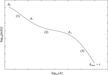
are to be determined from conservation laws and scaling arguments. The number density is shown schematically in figure 1 with ranges (1)–(3) labelled. Also indicated are the characteristic forcing-scale vortex area
 $A_{f}$
and maximum vortex area
 $A_{max}$
, together with the transition regions
 $A_{-}$
and
 $A_{+}$
that demarcate the intermediate range (2).
Before formulating a theory for the proposed scaling ranges, we introduce the concept of a ‘comoving’ interval in
 $A$
-space. In contrast to a fixed interval,
 $[\unicode[STIX]{x1D707}A_{0},A_{0}]$
, where
 $\unicode[STIX]{x1D707}<1$
and
 $A_{0}$
are constant in time, it is convenient to define the ‘comoving’ interval
 $[\unicode[STIX]{x1D707}A_{0}(t),A_{0}(t)]$
whose endpoints evolve at the vortex growth rate. Individually, vortices do not progress smoothly towards larger scales; they may jump from scale to scale and even decrease in size as a result of mergers. However, statistically speaking we picture an ‘average’ vortex as increasing in size continually at the vortex growth rate. In a comoving interval one imagines following such a statistical vortex as it grows in size and moves through
 $A$
-space towards larger scales. We assume that statistical vortices in all three ranges grow in area at the same rate, given by the similarity law
 $a(t)\sim t^{1/2}$
following from (2.3) above.
In terms of scale invariance, we expect conservation laws to hold in comoving intervals because the system should be invariant under the length scale dilatation associated with the inverse cascade as manifested through vortex growth. The particular type of invariance, and hence the conserved quantity, depends on the dynamics of the scaling range.
Schematic of a three-part number density
 $n(A)$
, with forcing-scale area
 $A_{f}$
, transitional areas
 $A_{-}$
and
 $A_{+}$
, and maximum vortex area
 $A_{max}$
labelled.

We now discuss the three proposed scaling regimes obtained by considering conservation of
 $E_{v}$
,
 $Z_{v}$
and
 $N_{v}$
, respectively, in comoving intervals.
(1) We call this regime the ‘thermal bath’. It extends over the range
 $A_{f}<A<A_{-}$
, and is ‘pinned’ at one end to the forcing scale
 $A_{f}$
and equilibrated with the forcing, which injects energy at a constant rate. Because this range is equilibrated, we expect
 $\overline{\unicode[STIX]{x1D714}_{v}^{2}}$
to be time-invariant, and
 $\unicode[STIX]{x1D70E}_{v}$
,
 $N_{v}$
,
 $Z_{v}$
and
 $E_{v}$
all to be constant in the fixed interval
 $[\unicode[STIX]{x1D707}A_{0},A_{0}]$
. This sets
 $\unicode[STIX]{x1D6FC}_{1}=0$
. We also expect conservation of
 $E_{v}^{cm}$
in an interval
 $[\unicode[STIX]{x1D707}A_{0}(t),A_{0}(t)]$
comoving with the vortex area growth rate, where again
 $\unicode[STIX]{x1D707}<1$
is a constant factor. This requirement is the analogue of
 $k$
-independent energy flux through energy-cascading subranges in two-dimensional turbulence, except that here we are not working in
 $k$
-space, but in
 $A$
-space, and the flux is restricted to the vortex subfield. Conservation of
 $E_{v}^{cm}$
then implies
 $r_{1}=3$
, so that
 $$\begin{eqnarray}\displaystyle E_{v}^{cm}=\frac{1}{2{\mathcal{D}}}\int _{\unicode[STIX]{x1D707}A_{0}(t)}^{A_{0}(t)}\overline{\unicode[STIX]{x1D714}_{v}^{2}}A^{2}n(A)\,\text{d}A\sim \int _{\unicode[STIX]{x1D707}A_{0}(t)}^{A_{0}(t)}A^{-1}\,\text{d}A\sim -\log \unicode[STIX]{x1D707}\sim t^{0}. & & \displaystyle\end{eqnarray}$$
From (3.4), using
 $A_{0}(t)\sim t$
, and assuming
 $\overline{\unicode[STIX]{x1D714}_{v}^{2}}$
is constant, it follows that
 $$\begin{eqnarray}\displaystyle Z_{v}^{cm}\sim t^{-1},\quad N_{v}^{cm}\sim t^{-2}. & & \displaystyle\end{eqnarray}$$
(2) In the intermediate scaling regime, which extends over the range
 $A_{-}<A<A_{+}$
, we posit a self-similar distribution of vortex sizes, which constrains the number density
 $n(A)$
. Vortices in a comoving interval occupy an area
 $$\begin{eqnarray}\displaystyle A_{v}=\int _{\unicode[STIX]{x1D707}A_{0}(t)}^{A_{0}(t)}An(A)\,\text{d}A. & & \displaystyle\end{eqnarray}$$
Scale invariance requires
 $A_{v}/A_{0}$
to be independent of
 $A_{0}$
, which is satisfied if
 $n(A)=c(t)/A$
(Dritschel et al.
Reference Dritschel, Scott, Macaskill, Gottwald and Tran2008). Though merger and filament shedding will occur in the forced scale-invariant range as in the decaying system, crucially in the forced system we expect enstrophy so lost to be replaced, so that
 $Z_{v}^{cm}$
is constant. This gives
 $$\begin{eqnarray}\displaystyle Z_{v}^{cm}=\frac{1}{2{\mathcal{D}}}\int _{\unicode[STIX]{x1D707}A_{0}(t)}^{A_{0}(t)}\overline{\unicode[STIX]{x1D714}_{v}^{2}}An(A)\,\text{d}A\sim c(t)\overline{\unicode[STIX]{x1D714}_{v}^{2}}A_{0}(t)\sim t^{0}, & & \displaystyle\end{eqnarray}$$
and since
 $A_{0}(t)\sim t$
for constant energy injection, we obtain
 $$\begin{eqnarray}\displaystyle c(t)\sim t^{-1}, & & \displaystyle\end{eqnarray}$$
where we have again assumed that
 $\overline{\unicode[STIX]{x1D714}_{v}^{2}}$
is constant in time. Equation (3.8) in turn yields
 $$\begin{eqnarray}\displaystyle E_{v}^{cm}\sim t,\quad N_{v}^{cm}\sim t^{-1}. & & \displaystyle\end{eqnarray}$$
The vortices grow in area faster than found in Dritschel et al. (Reference Dritschel, Scott, Macaskill, Gottwald and Tran2008) for the corresponding scale-invariant range in decaying two-dimensional turbulence, where
 $A(t)\sim t^{1/3}$
. The faster growth rate reflects a higher merger rate, which arises in the forced situation because enstrophy is continuously input into the system. The predicted
 $c(t)\sim t^{-1}$
decay of the vortex density in the case of time-invariant
 $\overline{\unicode[STIX]{x1D714}_{v}^{2}}$
is also faster than the
 $c(t)\sim t^{-2/3}$
found for decaying turbulence with constant
 $\overline{\unicode[STIX]{x1D714}_{v}^{2}}$
by Dritschel et al. (Reference Dritschel, Scott, Macaskill, Gottwald and Tran2008); again, the difference arises because the vortex merger rate is higher in the forced system.
(3) This is the ‘front’ of the vortex population, in which vortices populate new and larger scales. In this regime the vortices are large and spaced far apart; we assume that they move relatively freely of each other, interact little and merge with other large vortices only rarely. These considerations suggest that, again for constant
 $\overline{\unicode[STIX]{x1D714}_{v}^{2}}$
, the number of vortices
 $N_{v}$
in a range of scales
 $[\unicode[STIX]{x1D707}A_{0}(t),A_{0}(t)]$
comoving with the vortex area growth rate
 $A_{0}\sim t$
should remain constant. It now follows that
 $$\begin{eqnarray}\displaystyle E_{v}^{cm}\sim t^{2},\quad Z_{v}^{cm}\sim t. & & \displaystyle\end{eqnarray}$$
Integrating
 $N_{v}^{cm}$
as above gives the condition
 $\unicode[STIX]{x1D6FC}_{3}=r_{3}-1$
. Unlike in ranges (1) and (2), there is no immediately obvious feature of the large-scale flow that provides a further constraint on
 $\unicode[STIX]{x1D6FC}_{3}$
and
 $r_{3}$
. In this range of scales, we imagine that vortices are so sparse that they are effectively point objects, merging relatively infrequently at just the rate needed to maintain the front propagation. Because of the hypothesized lower merger rate we expect vortices to accumulate at fixed
 $A$
, resulting in a significantly steeper slope than in the intermediate range. The numerical results below suggest that
 $r_{3}\approx 6$
,
 $\unicode[STIX]{x1D6FC}_{3}\approx 5$
, consistent with this argument and the constraint
 $\unicode[STIX]{x1D6FC}_{3}=r_{3}-1$
obtained above.
In summary, we predict a vortex number density of the form
 $$\begin{eqnarray}\displaystyle n(A,t)\sim \left\{\begin{array}{@{}ll@{}}A^{-3},\quad & A_{f}\leqslant A<A_{-},\\ t^{-1}A^{-1},\quad & A_{-}<A<A_{+},\\ t^{r_{3}-1}A^{-r_{3}},\quad & A_{+}<A\leqslant A_{max},\end{array}\right. & & \displaystyle\end{eqnarray}$$
where
 $A_{-}$
and
 $A_{+}$
are time-evolving transitional vortex areas. Matching the number densities at
 $A_{-}$
and
 $A_{+}$
yields
 $$\begin{eqnarray}\displaystyle A_{-}\sim t^{1/2},\quad A_{+}\sim t^{r_{3}/(r_{3}-1)}. & & \displaystyle\end{eqnarray}$$
The above predictions are obtained under the assumption that
 $\overline{\unicode[STIX]{x1D714}_{v}^{2}}$
is constant in time. If we instead allow for a more general time evolution of
 $\overline{\unicode[STIX]{x1D714}_{v}^{2}}$
, similar scaling arguments give a modified three-part number density of the form
 $$\begin{eqnarray}\displaystyle n(A,t)\sim \left\{\begin{array}{@{}ll@{}}A^{-3},\quad & A_{f}\leqslant A<A_{-},\\ \overline{\unicode[STIX]{x1D714}_{v}^{2}}^{-1}t^{-1}A^{-1},\quad & A_{-}<A<A_{+},\\ \overline{\unicode[STIX]{x1D714}_{v}^{2}}^{-1}t^{r_{3}-1}A^{-r_{3}},\quad & A_{+}<A\leqslant A_{max}.\end{array}\right. & & \displaystyle\end{eqnarray}$$
Further allowing
 $\overline{\unicode[STIX]{x1D714}_{v}^{2}}$
to evolve differently in ranges (2) and (3) gives transitional areas that evolve as
 $$\begin{eqnarray}\displaystyle A_{-}\sim (\overline{\unicode[STIX]{x1D714}_{v}^{2}})_{2}^{1/2}t^{1/2},\quad A_{+}\sim \left[\frac{(\overline{\unicode[STIX]{x1D714}_{v}^{2}})_{2}}{(\overline{\unicode[STIX]{x1D714}_{v}^{2}})_{3}}\right]^{1/(r_{3}-1)}t^{r_{3}/(r_{3}-1)}, & & \displaystyle\end{eqnarray}$$
where the subscripts on
 $(\overline{\unicode[STIX]{x1D714}_{v}^{2}})_{2}$
and
 $(\overline{\unicode[STIX]{x1D714}_{v}^{2}})_{3}$
denote the range. We will discuss the case for time-evolving
 $\overline{\unicode[STIX]{x1D714}_{v}^{2}}$
in the following section.
4 Numerical verification
We simulate the dynamics governed by
 $$\begin{eqnarray}\displaystyle \unicode[STIX]{x2202}_{t}\unicode[STIX]{x1D714}+J(\unicode[STIX]{x1D713},\unicode[STIX]{x1D714})=f+d & & \displaystyle\end{eqnarray}$$
in a doubly periodic domain using a traditional pseudospectral method. Here
 $\unicode[STIX]{x1D714}=-\unicode[STIX]{x1D6FB}^{2}\unicode[STIX]{x1D713}$
, where
 $\unicode[STIX]{x1D713}$
is the streamfunction and
 $\unicode[STIX]{x1D714}$
is the vorticity,
 $J(\unicode[STIX]{x1D713},\unicode[STIX]{x1D714})$
is the two-dimensional Jacobian,
 $f$
is forcing and
 $d$
is dissipation. We ran an ensemble of 10 simulations at resolution
 $8192^{2}$
forced at
 $k_{f}=1024$
. The initial condition is a state of no flow. The forcing is
 $\unicode[STIX]{x1D6FF}$
-correlated in time, and we use a narrow-band forcing such that
 $$\begin{eqnarray}\displaystyle \hat{f}(\boldsymbol{k})=\left\{\begin{array}{@{}ll@{}}\displaystyle \sqrt{\frac{\unicode[STIX]{x1D700}_{I}k}{2\unicode[STIX]{x03C0}\unicode[STIX]{x0394}k\,\text{d}t}},\quad & |k-k_{f}|\leqslant \unicode[STIX]{x0394}k,\\ 0,\quad & |k-k_{f}|>\unicode[STIX]{x0394}k,\end{array}\right. & & \displaystyle\end{eqnarray}$$
where
 $\hat{f}$
is the Fourier transform of
 $f$
,
 $\unicode[STIX]{x1D700}_{I}$
is the injected energy,
 $\text{d}t$
is the time step and
 $\unicode[STIX]{x0394}k$
sets the forcing bandwidth. The forcing satisfies
 $\langle \hat{f}(\boldsymbol{k})\hat{f}(\boldsymbol{k})^{\ast }\rangle =\unicode[STIX]{x1D700}_{I}/\unicode[STIX]{x03C0}k$
and yields an energy injection rate
 $\unicode[STIX]{x1D700}_{I}$
. Here we set
 $\unicode[STIX]{x0394}k=4$
and
 $\unicode[STIX]{x1D700}_{I}=1$
.
The viscous term is of the form
 $d=(-1)^{s+1}\unicode[STIX]{x1D708}\unicode[STIX]{x1D6FB}^{2s}\unicode[STIX]{x1D714}$
, where
 $s$
is the order of hyperviscosity and
 $\unicode[STIX]{x1D708}$
is the strength, and we set
 $s=4$
. In our simulations there is no linear drag or hypoviscosity at large scales and the vortex formation found is therefore not a hypoviscous effect. This absence of large-scale dissipation means the cascade is quasi-steady: though the spectral peak moves towards large scales, the energy spectrum varies only slowly in the inertial range, with the variation due solely to the evolution of the vortex population. Preliminary analysis indicates that a vortex population also forms under more general forcing and dissipation conditions, including broadband forcing and Laplacian viscosity.
Vortices are selected with the simplest possible procedure: regions with
 $\unicode[STIX]{x1D714}\geqslant 2\unicode[STIX]{x1D714}_{rms}$
are identified, and those with
 $A\geqslant A_{min}$
, where
 $A_{min}=\unicode[STIX]{x03C0}r_{min}^{2}$
and
 $r_{min}=\unicode[STIX]{x03C0}/(k_{f})$
, are retained and classified as coherent, while regions with
 $\unicode[STIX]{x1D714}<2\unicode[STIX]{x1D714}_{rms}$
and/or
 $A<A_{min}$
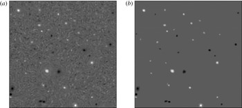
are classified as part of the background. The restriction on minimum area ensures that vortices are at or larger than the forcing scale. The addition of an eccentricity criterion had negligible effect on the extracted coherent field. Though simple, our selection procedure reliably identifies intense, nearly circular, long-lived vortices, and is sufficient for our focus on physical space characteristics. The total (a) and coherent (b) vorticity fields on a
 $384\times 384$
subdomain (0.22 % of the domain) at
 $t=3.1$
are shown in figure 2. Vortices of various sizes are evident.
Total (a) and coherent (b) vorticity fields in a
 $384\times 384$
region (0.22 % of the domain) at
 $t=3.1$
. Black is negative and white positive vorticity.

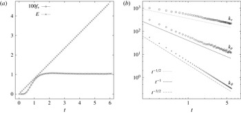
(a) Energy
 $E$
and percentage
 $100f_{v}$
of the domain occupied by inverse-cascade-scale coherent vortices. (b) Wavenumbers associated with the largest vortex
 $k_{v}$
(
 $\boxdot$
), spectral peak
 $k_{p}$
(
 $\odot$
) and streamfunction
 $k_{\unicode[STIX]{x1D713}}$
(
 $+$
) with their predicted growth laws.

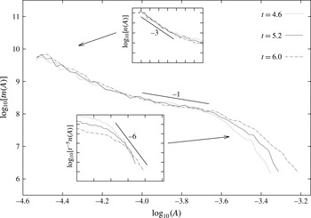
Rescaled number density
 $tn(A)$
(main panel) as a function of
 $A$
at the indicated times. The lower inset shows range (3) collapsed by the scaling
 $t^{-5}n(A)$
, and the upper inset shows the thermal bath range with no overall scaling. Thick solid lines proportional to
 $A^{-3}$
(upper inset),
 $A^{-1}$
(main panel) and
 $A^{-6}$
(lower inset) are shown for comparison.

Vortex self-energy
 $E_{v}^{cm}$
(a), enstrophy
 $Z_{v}^{cm}$
(b), vortex number
 $N_{v}^{cm}$
(c) and
 $\overline{\unicode[STIX]{x1D714}_{v}^{2}}$
-weighted vortex number
 $\unicode[STIX]{x1D70E}_{v}^{cm}$
(d) integrated over comoving intervals
 $[\unicode[STIX]{x1D707}A_{0}(t),A_{0}(t)]$
in ranges (1–3), with slope lines for comparison.

Logarithm of vortex mean square vorticity
 $\overline{\unicode[STIX]{x1D714}_{v}^{2}}$
as a function of
 $\text{log}_{10}(A)$
at the indicated times, and compensated by
 $t^{0}$
(a),
 $t^{-1/3}$
(b) and
 $t^{-2/3}$
(c).

Figure 3(a) shows the total flow energy
 $E$
and the area fraction
 $f_{v}$
occupied by coherent vortices. The energy grows like
 $t$
, as prescribed, and, once the vortex population is established, the prediction that the area fraction
 $f_{v}$
given by (3.2) is constant in time is well supported. The measured wavenumbers
 $k_{v}$
and
 $k_{p}$
corresponding to the largest vortex diameter (
 $\boxdot$
) and the spectral peak (
 $\odot$
), respectively, both averaged over the 10-member ensemble, are shown in figure 3(b), together with their predicted growth laws from (2.3)–(2.5). Also shown is the large-scale wavenumber
 $k_{\unicode[STIX]{x1D713}}=2\unicode[STIX]{x03C0}/l_{\unicode[STIX]{x1D713}}$
(
 $+$
) obtained from the measured value of
 $E$
. The measured wavenumbers
 $k_{v}$
and
 $k_{p}$
follow the predicted growth rates well over a substantial time interval.
The vortex number density is shown in figure 4. In the main panel we show the rescaled density
 $tn(A)$
: while not perfect, this scaling collapses the curves to a reasonable degree throughout the intermediate range (2), supporting the prediction (3.3). The upper inset shows the thermal bath range (1), in which the curves collapse with no overall time scaling, and the density follows an approximate law
 $n(A)\sim A^{-3}$
, as predicted. In the lower inset we show the front of the cascade, range (3), compensated by the temporal scaling
 $t^{-5}$
, which again collapses the curves to a reasonable degree, supporting (3.3). The collapse is not as good as in ranges (1) and (2), but this is not surprising given the short range of scales available and the relatively low occupation numbers of these bins. The slope in this range is approximately
 $-6$
, consistent with the requirement
 $\unicode[STIX]{x1D6FC}_{3}=r_{3}-1$
obtained from conservation of vortex number in this range. Refinements to the temporal scaling in ranges (2) and (3) are considered further below.
To verify the conservation laws introduced in § 3, we integrated
 $E_{v}$
,
 $Z_{v}$
,
 $N_{v}$
and
 $\unicode[STIX]{x1D70E}_{v}$
over comoving intervals
 $[\unicode[STIX]{x1D707}A_{0}(t),A_{0}(t)]$
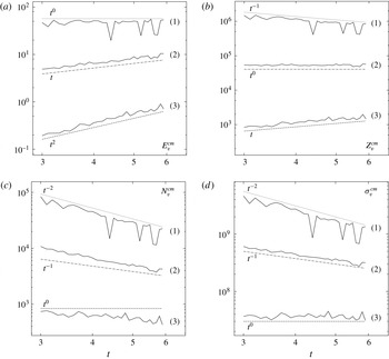
in each of the ranges (1), (2) and (3) separately. The results are shown in figure 5. Although the data are noisy, they broadly support the conservation laws proposed in § 3, particularly in regimes (1) and (2), which conserve
 $E_{v}^{cm}$
and
 $Z_{v}^{cm}$
, respectively, as shown in figure 5(a,b). These panels also indicate that both
 $E_{v}^{cm}$
and
 $Z_{v}^{cm}$
evolve according to the predictions (3.5), (3.9) and (3.10) derived in the other ranges.
The conservation of
 $N_{v}^{cm}$
in range (3) and its time evolution in range (2) are less well supported (figure 5
c). Measured values suggest a scaling closer to
 $N_{v}^{cm}\sim t^{-4/3}$
in range (2) and
 $N_{v}^{cm}\sim t^{-2/3}$
in range (3). As discussed in § 3, the most relevant conserved quantity may not be the raw vortex number, but rather
 $\unicode[STIX]{x1D70E}_{v}$
, the vortex number weighted by the vortex mean square vorticity
 $\overline{\unicode[STIX]{x1D714}_{v}^{2}}$
, as defined in § 3. We turn next to the analysis of
 $\overline{\unicode[STIX]{x1D714}_{v}^{2}}$
and its temporal evolution in our simulations.
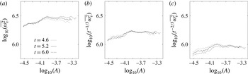
Figure 6(a) shows the vortex mean square vorticity
 $\overline{\unicode[STIX]{x1D714}_{v}^{2}}$
plotted against area
 $A$
at the same three times considered in figure 4. At all times
 $\overline{\unicode[STIX]{x1D714}_{v}^{2}}$
shows very weak dependence on
 $A$
, in the sense that variations around the mean value are small relative to that value, supporting the arguments made above for
 $A$
-independent
 $\overline{\unicode[STIX]{x1D714}_{v}^{2}}$
, and additionally consistent with previous studies of the vortex population in freely decaying turbulence (Dritschel et al.
Reference Dritschel, Scott, Macaskill, Gottwald and Tran2008).
Considering next the temporal dependence, figure 6(a) also indicates a small but systematic increase of
 $\overline{\unicode[STIX]{x1D714}_{v}^{2}}$
in time. This time dependence in fact accounts very well for the discrepancy in the scaling of
 $N_{v}$
noted above, and represents a potentially important refinement to the theory. In the absence of a theoretical prediction, however, we restrict the discussion here to empirically determining the growth of
 $\overline{\unicode[STIX]{x1D714}_{v}^{2}}$
based on the current data. As a first step, we compensate
 $\overline{\unicode[STIX]{x1D714}_{v}^{2}}$
by the factors
 $t^{-1/3}$
and
 $t^{-2/3}$
(figure 6
b,c). The first compensation (
 $t^{-1/3}$
) collapses the curves at intermediate scales, while the second (
 $t^{-2/3}$
) approximately collapses the curves in the large-scale regime, albeit not as well and over a shorter range, again consistent with the relative paucity of data at these scales.
Logarithms of the transitional areas
 $A_{-}$
and
 $A_{+}$
, together with best-fitting slope lines.

Assuming, then, a tentative scaling of
 $\overline{\unicode[STIX]{x1D714}_{v}^{2}}=(\overline{\unicode[STIX]{x1D714}_{v}^{2}})_{2}\sim t^{1/3}$
in the intermediate range (2) and a scaling of
 $\overline{\unicode[STIX]{x1D714}_{v}^{2}}=(\overline{\unicode[STIX]{x1D714}_{v}^{2}})_{3}\sim t^{2/3}$
in the large-scale range (3), we return to the analysis of the conserved quantities in these ranges and make the following two refinements: (i) in range (2), conservation of
 $Z_{v}$
now implies
 $\unicode[STIX]{x1D70E}_{v}\sim t^{-1}$
and
 $N_{v}\sim (\overline{\unicode[STIX]{x1D714}_{v}^{2}})_{2}^{-1}t^{-1}\sim t^{-4/3}$
; (ii) in range (3), conservation of
 $\unicode[STIX]{x1D70E}_{v}$
rather than
 $N_{v}$
now implies
 $N_{v}\sim (\overline{\unicode[STIX]{x1D714}_{v}^{2}})_{3}^{-1}\sim t^{-2/3}$
. These decay rates are consistent with the empirically observed decay of
 $N_{v}^{cm}$
seen in figure 5(c) and discussed above. All other scaling predictions are unchanged by this refinement. In figure 5(d), we show the measured quantity
 $\unicode[STIX]{x1D70E}_{v}$
in the three ranges, together with these predicted slopes. The quantity
 $\unicode[STIX]{x1D70E}_{v}$
follows the temporal scaling laws originally predicted for
 $N_{v}$
in the three ranges noticeably better than the vortex number
 $N_{v}$
itself follows these scalings.
The measurements
 $(\overline{\unicode[STIX]{x1D714}_{v}^{2}})_{2}\sim t^{1/3}$
and
 $(\overline{\unicode[STIX]{x1D714}_{v}^{2}})_{3}\sim t^{2/3}$
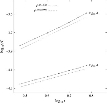
obtained from the compensated plots above are very approximate, but are consistent with a number of aspects of the simulations. For further support of their numerical values, we measured the growth of
 $\overline{\unicode[STIX]{x1D714}_{v}^{2}}$
indirectly by comparing estimates of the transitional areas
 $A_{\pm }$
with the prediction (3.14). Estimates of
 $A_{\pm }$
were obtained by computing the intersection of lines of slope
 $-3$
and
 $-1$
fitted through the thermal bath and intermediate scaling ranges of the number density and the intersection of lines of slope
 $-1$
and
 $-6$
fitted through the intermediate and large-scale ranges. This was done at times
 $t=3.0,3.5,\ldots ,5.5,6.0$
, and the resulting values for
 $A_{\pm }$
are shown in figure 7. A nonlinear least-squares fit to the measured values gives growth laws of
 $A_{-}\sim t^{0.659\pm 0.006}$
and
 $A_{+}\sim t^{1.16\pm 0.02}$
, where the uncertainty given is the asymptotic standard error of the fit. Although the uncertainty obtained is an underestimate, as it neglects the error inherent in fitting slope lines to
 $n(A)$
, comparison with (3.14) is supportive of the growth rates
 $(\overline{\unicode[STIX]{x1D714}_{v}^{2}})_{2}\sim t^{1/3}$
and
 $(\overline{\unicode[STIX]{x1D714}_{v}^{2}})_{3}\sim t^{2/3}$
obtained above. In particular, figure 7 provides evidence that the
 $\overline{\unicode[STIX]{x1D714}_{v}^{2}}$
correction is necessary, since there are clear departures from the uncorrected prediction (3.12).
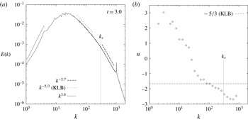
The ensemble-averaged energy spectrum (figure 8
a) for
 $t=3.0$
is steeper than
 $k^{-5/3}$
over the vortex-containing range, with a slope of approximately
 $-2.7$
. In the range
 $[k_{f},k_{v}]$
, where
 $k_{v}$
is the wavenumber associated with the diameter of the largest vortex, we expect
 $E(k)$
to be dominated by the vortex cores, while at larger scales vortex configurations will become important. The scaling clearly changes at the transition wavenumber
 $k_{v}$
, and for
 $k<k_{v}$
the spectrum shallows to approximately
 $k^{-5/3}$
. Slopes computed over equal intervals in
 $\text{log}(k)$
(figure 8
b) show the detailed behaviour over the range
 $k<900$
. There is a short
 $-5/3$
plateau at
 $k\approx 100$
, and the slope at low
 $k$
is approximately
 $3$
, providing verification that domain effects are unimportant (Lowe & Davidson Reference Lowe and Davidson2005; Tran & Dritschel Reference Tran and Dritschel2006). Later in the simulation at
 $t=6.0$
(not shown), the energy spectrum in the range
 $k>k_{p}$
has much the same shape and scaling: the vortex-containing and
 $-5/3$
ranges have extended, but the slopes are unchanged, indicating that domain-scale effects still have yet to influence the inertial range.
Energy spectrum
 $E(k)$
with
 $k^{-2.7}$
(dash-dotted),
 $k^{-5/3}$
(large dotted) and
 $k^{3}$
(small dotted) lines for comparison (a), and local slope averaged over equal intervals in
 $\text{log}(k)$
(b). The wavenumber
 $k_{v}$
corresponding to the largest vortex is indicated.

5 Conclusion
We propose a new similarity theory for the forced two-dimensional inverse cascade based on a population of coherent vortices that dominates the vorticity field at scales larger than the forcing scale. Similarity arguments predict growth rates for the largest vortex in physical space and for the peak of the energy spectrum in wavenumber space. A key part of the theory is the existence of a three-part number density, whose scaling and evolution are derived by considering the transport, mediated by vortex merger within the vortex population, of conserved quantities between the forcing scale and the scale of the largest vortex. Our theory may be considered as an extended forced counterpart of the freely decaying vortex theory of Dritschel et al. (Reference Dritschel, Scott, Macaskill, Gottwald and Tran2008). Although, by the introduction of a scale associated with the largest vortex, the presence of coherent vortices breaks traditional assumptions of scale invariance in the inverse energy cascade, the population itself retains elements of that scale invariance in a physical-space context. The scaling and statistics of the vortex population are robust and the derivation of its evolution from time-honoured principles of material vorticity conservation and scale invariance is in keeping with traditional turbulence research.
The physical-space phenomenology and predicted scaling exponents of the theory are supported by high-resolution numerical simulations, which confirm that, far from being artefacts or peculiarities of forcing or diffusion, coherent vortices are an integral part of the two-dimensional inverse cascade. The simulations also support the key assertions behind the theory, namely independence of mean square vorticity across area, and the conservation of vortex energy, enstrophy and number through vortex area space. Details of the simulations also point towards an important potential modification to the theory, which should take into account a small but systematic temporal variation of mean square vorticity to correctly predict the evolution of the vortex number density and transitional areas
 $A_{-}$
and
 $A_{+}$
between scaling ranges. Current work is under way to understand whether such a modification is an intrinsic part of the theory, or arises here due to inherent limitations of the numerical simulations.
Finally, we note that the scale of the largest vortex is always less than the scale of the peak of the energy spectrum in physical space. This suggests the possibility of a two-part structure of the inverse cascade, in which scales below that of the largest vortex are described most naturally in terms of the vortex population, while scales larger than that of the largest vortex may be described in terms of traditional phenomenology. The two-part nature of the spectrum shown in figure 8 supports this to the extent permitted by the numerical constraints. However, an intriguing possibility is that the inverse energy cascade at scales larger than the largest vortex may nonetheless be influenced by the dynamics of the vortex population, in particular by the tendency of vortices to cluster into groups of like sign. An effective theory of the entire inverse cascade based on vortex interactions in the three number density scaling ranges may thus be possible. Further research will explore this possibility and examine how clustering of the coherent vortex population influences flow dynamics at scales between the largest vortex and the spectral peak.
Acknowledgements
Simulations were run on the St Andrews MHD Cluster. The authors thank D. Dritschel for useful discussions and The Fields Institute for funding to attend the Workshop on Extreme Events and Criticality in Fluid Mechanics, where part of this work was completed. B.H.B. is supported by the Natural Environment Research Council grant NE/M014983/1.