


1. INTRODUCTION
This paper studies the reciprocal causality between migration and the incidence of disease. While it is well known that migration can contribute to spreading diseases through the effect of crowding, we study its consequences for the composition of populations, which, in turn, affects the evolution of disease. If migration responds to disease incidence as well as influences it, feedback effects may either dampen or magnify initial differences in disease prevalence between locations. We show in particular how, for a large class of infectious endemic diseases, migration can magnify initial differences, since the healthy have a stronger incentive than the sick to flee unhealthy neighborhoods. This can turn some localities into “sinks” whose initial high disease prevalence attracts further sick individuals because they cannot compete with healthy individuals for scarce space in healthier localities. We show that several steady states can exist with different degrees of segregation of sick and healthy individuals. In fact, higher segregation is beneficial in the model, since it unambiguously reduces prevalence in low-prevalence locations and does not necessarily increase it in high-prevalence locations. This has implications for public policy towards migration and may provide a case for encouraging or even subsidising migration that has such results.
Epidemiologists have already addressed how individual migration may contribute, among other factors, to the spread of diseaseFootnote 1 and a few studies have assessed its relative importance in malaria’s eradication in the Early twentieth Century United States (Barreca et al., Reference Barreca, Fishback and Kantor2011) or the contribution of forced migration to the incidence of malaria in refugee-receiving countries (Montalvo and Reynal-Querol, Reference Montalvo and Reynal-Querol2007). But much less is known about how migration in turn responds to infectious diseases, although numerous historical instances have been recorded of people fleeing plague or other epidemics by migrating to distant areas (see McNeill, Reference McNeill1977) Footnote 2.
There is also abundant historical evidence of endemic disease as a factor in individuals’ location decisions. Historians have shown that infectious diseases causing high mortality rates among settlers were a key determinant of European colonization. Among other examples, Acemoglu et al. (Reference Acemoglu, Simon and Robinson2001) refer to Crosby (Reference Crosby1986 pp. 143–144) who has shown that the Pilgrim Fathers decided to migrate to the United States rather than to Guyana because of the high mortality rates from infectious diseases in Guyana. We also know from Alexis de Tocqueville and other witnesses of that period that it took the draining of the malarial swamps in the State of Michigan in the mid nineteenth century for the interior of the state to be opened up by settlers on a scale comparable to what had already occurred further west in IllinoisFootnote 3.
Even today, there is a vast difference between different parts of the world in the incidence of infectious disease. Mortality statistics published by the World Health OrganizationFootnote 4 reveal that deaths from infectious or parasitic disease make up just over 2% of all deaths in Europe, and some 3% of deaths in North America, while they make up over 52% of all deaths in Africa (9% of all deaths being due to malaria and 20% of all deaths being due to HIV/AIDS). The world average is a little under 20% of all deaths. Given the importance of infectious disease in mortality, it would be surprising if individuals did not take variations in its incidence into account in their location decisions. The location of some important cities (Nairobi in Kenya, for example, or Colombo in Sri Lanka) seems likely to have benefited from their low rates of malarial incidence compared to the rest of the country.
Obviously, there are correlations between high rates of disease prevalence and a high incidence of poverty, and the complex linkages between poverty and infectious disease make their interaction an interesting area of study. Economists have begun to study the channels through which health outcomes interact with economic factors (Bell and Gersbach, Reference Bell and Gersbach2006, Bell et al. Reference Bell, Devarajan and Gersbach2006, Duncan et al. Reference Duncan, Daly, McDonough and Williams2002, Hurd et al. Reference Hurd, Adams, McFadden, Merill and Ribeiro2003, Marmot, Reference Marmot2002). And there is strong evidence that epidemic outbreaks cause important economic lossesFootnote 5. Furthermore, asset markets may also be affected, as was observed on the housing market in Hong Kong after the SARS outbreak (Wong, Reference Wong2008). However, among these linkages, migration has attracted rather little attention and yet has been under increasing focus since the SARS outbreak in China.
This paper models how the decisions of individuals to live in different areas are determined both by the health environment, captured in our model by different prevalence rates of diseases, and by economic factors such as costs of living. To capture the costs of living or of any fixed asset or amenity attached to a given area, the price of which increases with more people willing to settle in the area, we assume that there is a constant stock of land in each city and that rents will vary to clear the market for land.Footnote 6 This requires of course a dynamic set-up where the economic and health environment are affected by migration, and in turn determine individual decisions such as migration.
At the beginning of each period, individuals find themselves in one of two cities, which differ in a number of characteristics including the prevalence of disease. The two cities could also be interpreted as countries or regions, or even in some circumstances as different sectors of the economy. Footnote 7 Individuals have characteristics of their own, and in the model we focus on their health status (wealth, which normally differs among individuals, is here assumed to be the same for all individuals in one city so as to focus attention on differences in health). These individuals must make decisions about whether to stay in their city of origin or to migrate to the other city, which determines their consumption levels and their risk of being infected in the future : the benefits of risk reduction must be balanced against the costs, which here comprise not just migration costs but also any difference in the cost of living in the two cities. Time is infinite and the significance of the future is summarized in terms of a value function whose parameters are the health status of the individual and the characteristics of the city where she lives, both of these considered at the start of the following period. Each individual’s decisions therefore involve balancing the impact of varying the migration choice on her current utility and her future discounted value function.
We assume that healthy individuals in any one city are ex ante identical in terms of risk of infection. In this respect, we differ from Mesnard and Seabright (Reference Mesnard and Seabright2009), where individuals differ in an individual risk parameter. As individuals may have more information than the health authorities about their probability of being infected, we showed that quarantine measures may have unexpected effects on the spread of diseases, as they may give too high or too low incentives to migrate. This comes from the fact that migrants exert an externality on other individuals living in the destination and origin areas, which depends on their own risk of having caught the disease. The type of externality outlined in that two period model affects the spread of disease in the short run – just after the outbreak of an epidemic disease. In contrast, in the present paper, we show that there is a qualitative difference between short run and long run externalities. When the costs of migration are prohibitively high, an individual living in a city with zero prevalence imposes a very large externality in the long run if she acquires an infectious disease, because the people she infects directly and indirectly lead to the disease eventually reaching a positive steady state prevalence. However, if the same individual can migrate to a high prevalence city, the long run externality he/she imposes is zero. The fact that migration may lead to a sorting of sick/healthy individuals to high/low infected areas, has thus important policy implications that are studied in the present paper.
We first present the model and then solve for a steady state in prevalence in circumstances where migration costs are sufficiently high to discourage migration both in and out of the steady state. As expected, we show that cities with a healthier environment will have lower disease prevalence rates.
Next, we examine the properties of the steady states when migration costs are sufficiently low that healthy individuals in the high prevalence city will wish to migrate to the low-prevalence city, thereby bidding up rents in that city and encouraging sick individuals to migrate in the opposite direction. Historically, there is good reason to think that segregation of neighborhoods by disease incidence has an important influence on the spatial composition of cities and countries, and that relative housing costs play an important part in this process. The East End of London was considered a sink of disease (as well as of other unsavory characteristics) and prosperous citizens paid considerable sums to live in the West End, which thanks to the prevailing (westerly) winds could escape the noxious odors emanating from the east more easily than the east could avoid those from the west (the winds were thought to transmit disease – through “miasma” – as well as foul odors). Thus, although we do not claim that the phenomena we model are the only or even the main influences of infectious diseases on migration, it seems likely that they help explain some important characteristics of the geography of development, past, and present.
We show that, if all sick individuals do thus migrate, the prevalence rate in the low-prevalence city declines to zero so that there are no more infected individuals and migration in the steady state no longer occurs. However, the possibility of migration is important because it removes potentially infectious individuals from the locality where they can infect the most other people. The possibility of migration strictly lowers steady-state prevalence levels, and, it is unambiguously desirable to reduce migration costs to make this possible.
Our prediction that migration may under certain conditions induce sorting by health status has obvious echoes of the literature on segregation by individuals induced by their demand for local public goods such as education. The idea that individuals might sort between locations according to their preferences for local public goods goes back to Tiebout (Reference Tiebout1956), and there is a substantial more recent literature exploring the conditions under which that sorting would result in segregation of households by income (see Ellickson, Reference Ellickson1971, for a pioneering contribution and Epple, Reference Epple2003, for an overview). As documented by Timmins (Reference Timmins2005), there is much controversy about the strength of such effects and about how to estimate them econometrically. Particular applications have included sorting by preference for education provision (see Bénabou, Reference Bénabou1996a, Reference Bénaboub, and Fernandez and Rogerson, Reference Fernandez and Rogerson1996). There is a sense in which our model here documents broadly similar effects, since the prevalence rate of a disease has the relevant characteristics of a public good (or more precisely a public bad).
A distinctive feature of our model is that cities are likely to be in different steady states depending on the level of migration costs, in some of which there is sorting by migration, and with endogenous differences in health status even in the equilibria without sorting. It is also true in our model, unlike in many public-good models, that some of these equilibria can be Pareto-ranked, and in particular that there exist equilibria with the possibility of sorting outside the steady state that dominate equilibria without that possibility. These features in our view cast useful light on the possible role of migration policies in selecting one equilibria.
The paper proceeds as follows. Section 2 presents the links to the literature on epidemiology. Section 3 presents the model, Section 4 explains how individuals make their decisions, Section 5 studies the steady-state equilibria and shows that the existence of one or the other equilibrium depends importantly on the level of migration costs. Section 6 discusses the policy implications and concludes.
2. LINKS TO THE LITERATURE ON EPIDEMIOLOGY
Related work on infectious diseases can be classified in three main strands. A first strand of the literature uses dynamic models of epidemic diseases to understand the effects of different policies on the evolution of infectious diseases. For example, Sethi (Reference Sethi1978) studies optimal quarantine programs, which are modeled as an exogenous decrease in the infectivity parameter characterizing a specific disease. One shortcoming of these papers is that they assume away any potential behavioral response to the policies/changes considered. However, there is growing evidence pointing out that individual behavior is key to explain the evolution of aggregate disease (see Auld Reference Auld2003, Reluga Reference Reluga2010 and Fenichel, Reference Fenichel, Wang, Onofrio and Manfredi2013).
Two further strands of the literature capture this key role of individual decisions.
Models of decisions where individuals are rational have mostly focused on preventive behaviors such as vaccine or safe sex adoption (Geoffard and Philipson Reference Geoffard and Philipson1996, Kremer Reference Kremer, Jaffe, Lerner and Stern2000, Philipson, Reference Philipson2000); or partner choice decision (Philipson, Reference Philipson2000, Dupas et al. Reference Dupas, Duflo and Kremer2014). These studies obtain the common result that centralized measures may be ineffective for a number of reasons overviewed by Chen and Toxvaerd (Reference Chen and Toxvaerd2014). For example, Geoffard and Philipson (Reference Geoffard and Philipson1996) show that if demand for prevention treatments such as vaccines is prevalence elastic initially successful public health efforts typically run into diminishing returns, not simply for technical reasons but because the decline of a disease discourages prevention. Similar considerations apply to the factors determining the adoption of means of contraception as barrier methods for sexually transmissible diseases, and a growing literature now focuses on the microeconomic determinants of such individual decisions, in order to reach a better understanding of epidemiological patterns (See Gersovitz and Hammer (Reference Gersovitz and Hammer2003, Reference Gersovitz and Hammer2004) and Pattanayak et al. (Reference Pattanayak, Poulos and Yang2007) for surveys of the evidence on the prevalence elasticity of preventive behavior).
The third strand of literature, which can be characterized as Behavioral Epidemiology, explores the consequences of individuals’ exposure to risk using models of bounded rationality or studies how information about disease or the value of treatments spreads via word-of-mouth learning (Medlock et al., Reference Medlock, Luz, Struchiner and Galvani2009; d’Onofrio et al., Reference d’Onofrio, Manfredi, Salinelli, d’Onofrio and Manfredi2013; Bauch et al., Reference Bauch, Onofrio, Manfredi, Onofrio and Manfredi2013; Fenichel and Wang, Reference Fenichel, Wang, Onofrio and Manfredi2013).
Although most of these studies appear to focus on a single aspect of epidemiology, namely preventive behaviors, they explore a wide range of behavior types with very different policy implications. Depending on whether individual decisions are complements such as for adoption of safe sex or substitutes such as for vaccination, interventions may have very different effects on the overall disease prevalence. In particular, when prevention leads to complementarities between individual utilities, multiple equilibria are possible. Our model will show that the decision to migrate displays similar properties, which leads to multiple equilibria and an interesting policy coordination issue.
To our knowledge, migration as a preventive behavior has not been studied before Mesnard–Seabright (Reference Mesnard and Seabright2009) and the effects of migration restrictions such as quarantine measures have been overlooked by the literature using decentralized decision making frameworks. Yet, as was observed in the aftermath of the Ebola crisis, individuals may respond to strict quarantine measures by moving to different areas, which may have unexpected effects on the evolution of diseases. In such circumstances, Mesnard–Seabright (Reference Mesnard and Seabright2009) highlighted potential unexpected effects of too strong quarantine measures pushing still asymptomatic but sick individuals to escape from the epicenter of an epidemic disease: individuals who are more accurately informed than the authorities about their previous exposure to infection, may choose to migrate “strategically” just after the outbreak of an epidemic disease into a low prevalence area while still asymptomatic, which entails negative externalities.
The present paper highlights another channel through which migration restrictions for controlling spread of infectious diseases may have undesirable effects. Even without asymmetric informational issues, we show that too strict migration restrictions may lead in the long run to an equilibrium with a higher overall prevalence rate of disease than without restrictions. Indeed, strong migration restrictions may distort the sorting of sick/healthy individuals to high/low infected areas.
3. THE MODEL
Consider a discrete time, infinite horizon model with two equally-sized cities in terms of population, indexed by i ∈ {1, 2}.Footnote 8 Since our purpose here is to capture externalities due to pure compositional effects, we focus on the fact that migration incentives in one direction create pressures for migration in the opposite direction because of resource constraints and adopt the simplifying assumption that populations are constant, and normalized to unityFootnote 9.
Y denotes the constant per-period exogenous income in both cities (income is an endowment, and agents are assumed identical in income).Footnote 10 Out of this income, individuals must pay a rent rit in the city in which they choose to live. To simplify the calculations, we assume that land is not scarce at the margin in the city with low rent, so that rit = 0 whenever rit < rjt. This means we can write rt ≡ rjt for the city with high rent. This rent will be endogenously determined by a land market that clears when the net demand of individuals for migration to the city with high rent is zero.
We assume that one city has a more disease-prone environment, which favors the spread of disease vectors (think for example of low altitude or a high degree of humidity, which may favor airborne or insect borne diseases). We will capture the degree of disease-proneness of city i’s environment by a parameter αi and assume, without loss of generality, that α1, α2 < 1, which ensures interior solutions by ruling out theoretically possible but empirically uninteresting cases of diseases which affect the entire population.
Each individual can be in two states of health, denoted by θ: sick (S) or healthy (H).Footnote 11 At time t, a proportion pit of city i’s population are sick, the proportion of healthy inhabitants being therefore (1 − pit). We call pit the “prevalence” of the disease in city i at time t. We assume that the parameters αi are such as to ensure that
 $$\begin{equation}
p_{1t}+p_{2t}<1
\end{equation}$$
to capture the fact that the sick are a minority of the total population.
There is an exogenous utility cost m of migrating from one city to the other. This represents any kind of costs, which, like psychological costs, may be non-monetary and directly affect individuals’ utility. Utility is separable in this cost and in a term U(ct, θt) that is increasing and weakly concave in consumption ct at time t.
The assumption that utility is separable in the migration cost greatly simplifies the calculations because the derivatives of utility with respect to rents and disease prevalence do not depend on whether an individual has migrated in any given period, but it is unlikely that the qualitative findings of the model turn importantly on this restriction.
At the beginning of each period, individuals observe their current health status. They also have perfect foresight of the values of all parameters and city-level endogenous variables (namely Y, m, p, and r). They choose whether or not to migrate to the other city and all individuals receive the incomes and pay the rents in the city they have chosen to live in and consume the residual.
Accordingly, individuals living in city i face a per period budget constraint:
 $$\begin{equation}
Y-r_{it}=c_{t}.
\end{equation}$$
The health status of individuals evolves as follows:
Healthy individuals’ likelihood of becoming infected increases with the local prevalence, pit, and the degree of disease-proneness of their environment:
 $$\begin{equation}
P\left[ \theta _{t+1}=S/\theta _{t}=H\right] =\alpha _{i}p_{it}.
\end{equation}$$
Sick individuals recover from the disease naturally with exogenous probability π.Footnote 12
 $$\begin{equation}
P\left[ \theta _{t+1}=H/\theta _{t}=S\right] =\pi .
\end{equation}$$
We assume π < α2 < α1 in order to focus on interior solutions (diseases with higher recovery rates never become established as endemic in the population).
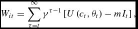
The expected present value of current and future utility of individuals of type θt in city i at time t is
 $$\begin{equation}
W_{it}=\sum _{\tau =t}^{\infty }\gamma ^{\tau -1}\left[ U\left( c_{t},\theta _{t}\right) -mI_{t}\right],
\end{equation}$$
where It is an indicator function taking the value 1 if they migrate in period t, otherwise 0.
We make the following assumptions about the effect of sickness on individual utilities:
Sickness lowers current welfare
 $$\begin{equation}
U\left( c_{t},S\right) \le U\left( c_{t},H\right).
\end{equation}$$
The marginal utility of consumption is independent of health status
 $$\begin{equation}
U^{\prime }\left( c_{t},H\right) =U^{\prime }\left( c_{t},S\right) \text{ for all }c_{t}.
\end{equation}$$
This assumption, it should be noted, implies (by integration of the function over a finite interval) that the utility cost of any given reduction in consumption depends only on the amount of the reduction in consumption and not on the health status of the individual experiencing it. Noting that utility is strictly monotonic in consumption, this assumption implies that, for any θi and θj,
 $$\begin{eqnarray}
U\left( Y,\theta _{i}\right) -U\left( Y-r_{i},\theta _{i}\right) >U\left( Y,\theta _{j}\right) -U\left( Y-r_{j},\theta _{j}\right) \text{ if and only if }r_{i}>r_{j}. \nonumber\\
\end{eqnarray}$$
In the context of our model, this has the consequence, as will be seen, that the healthy are willing to pay more than the sick to migrate to live near to other healthy people.Footnote 13 Our model should hence be seen as exploring the consequences in equilibrium of an empirically interesting phenomenon – namely the greater willingness of the healthy than the sick to migrate to live near other healthy people.
Note that we do not allow individuals to smooth consumption across time. Allowing for savings in our model would make each individual’s decisions in any period dependent on the entire history of their consumption decisions as well as on their entire medical history, which would greatly complexify the model with no extra gains for the understanding of our main results. As it is, individuals’ decisions are fully determined by their current health status and their city of residence, which gives us four distinct cases to study. We therefore write the objective function explicitly as a function of current health status as Wit(θt).
4. INDIVIDUAL DECISIONS
We first note that the objective function can be rewritten as follows, where i is the individual’s city at the beginning of the period and k is the city in which she chooses to live:
 $$\begin{eqnarray}
W_{it}\left( \theta _{t}\right) =U\left( Y-r_{kt},\theta _{t}\right) -mI_{t}+\gamma \sum \limits _{\theta _{t+1}}W_{kt+1}\left( \theta _{t+1}\right) P\left( \theta _{t+1}|\theta _{t}\right),\end{eqnarray}$$
where It = 1 if i ≠ k and 0 otherwise.
From this, it follows that Wit(θt) is strictly increasing in Y and strictly decreasing in rkt, and weakly decreasing in m.
Next, for each value of the current health status, we compare the utility of each individual in case she chooses not to migrate to the utility in case she migrates.
4.1. Individual Migration Choices
A healthy individual who chooses not to migrate and for whom therefore k = i will obtain utility VNit(H), which is equal to
 $$\begin{equation}
V_{it}^{N}(H)=U\left( Y-r_{it},H\right) +\gamma \alpha _{i}p_{it}W_{it+1}(S)+\gamma (1-\alpha _{i}p_{it})W_{it+1}(H).
\end{equation}$$
A healthy individual who chooses instead to migrate will obtain utility VMit(H), which is equal to
 $$\begin{eqnarray}
V_{it}^{M}(H)=U\left( Y-r_{jt},H\right) -m+\gamma \alpha _{j}p_{jt}W_{jt+1}(S)+\gamma (1-\alpha _{j}p_{jt})W_{jt+1}(H)). \nonumber\\
\end{eqnarray}$$
The agent who is currently sick and chooses not to migrate will receive utility VNit(S), which is equal to
 $$\begin{equation}
V_{it}^{N}(S)=U\left( Y-r_{it},S\right) +\gamma \pi W_{it+1}\left( H\right) +\gamma \left( 1-\pi \right) W_{it+1}\left( S\right).
\end{equation}$$
A sick individual who chooses instead to migrate from city i to city j will obtain utility VMit(S), which is equal to
 $$\begin{equation}
V_{it}^{M}(S)=U\left( Y-r_{jt},S\right) -m+\gamma \pi W_{jt+1}\left( H\right) +\gamma \left( 1-\pi \right) W_{jt+1}\left( S\right).
\end{equation}$$
Consequently, the condition for healthy individuals to migrate rather than to remain in their city of origin can be written as VMit(H) − Vit N(H) ⩾ 0, or written out in full as
 $$\begin{eqnarray}
0 &\le &U\left( Y-r_{jt},H\right) -U\left( Y-r_{it},H\right) -m+\gamma \alpha _{j}p_{jt}W_{jt+1}(S)-\gamma \alpha _{i}p_{it}W_{it+1}(S) \nonumber \\
&&+\gamma (1-\alpha _{j}p_{jt})W_{jt+1}(H)-\gamma (1-\alpha _{i}p_{it})W_{it+1}(H).
\end{eqnarray}$$
Similarly, the condition for sick individuals to migrate, VMit(S) − Vit N(S) ⩾ 0, can be written as out in full as
 $$\begin{eqnarray}
0 &\le &U\left( Y-r_{jt},S\right) -U\left( Y-r_{it},S\right) -m+\gamma \pi \left( W_{jt+1}\left( H\right) -W_{it+1}\left( H\right) \right) \nonumber \\
&&+\gamma \left( 1-\pi \right) \left( W_{jt+1}\left( S\right) -W_{it+1}\left( S\right) \right)
\end{eqnarray}$$
and we note that the conditions (13) and (14) are more likely to be fulfilled as rit − rjt increases and as m decreases, as we would expect.
4.2. Migration Flows
Denote by sjt (hjt), the proportion of the sick (healthy) who migrate from j to i in period t.
The proportions sit, sjt, hit, and hjt of individuals of each type migrating from one city to the other result from aggregating individual migration decisions shown by the equations (13) and (14). Hence, they are determined by the level of migration costs, by the differential in rental rates, which clear the market for land and by the differential in disease prevalences. Specifically, if inequality (14) does not hold, sit = 0, while if it holds with strict inequality then sit = 1. Likewise, if inequality (13) does not hold, hit = 0, while if it holds with strict inequality then hit = 1.
We know that those falling sick in any period on a given city consist of those previously healthy in the same city who have not migrated outwards and have fallen sick, plus any previously healthy in the other city who have migrated inwards and have fallen sick, plus those previously sick in the other city who have migrated inwards and have not recovered, plus those who were previously sick in the same city who have not migrated and who have not recovered. We can therefore write the equations governing the evolution of prevalence rates in the two cities as follows:
 $$\begin{eqnarray}
p_{it+1}&=&(1-\pi )p_{it}(1-s_{i,})+\alpha _{i}p_{it}(1-p_{it})(1-h_{it})\nonumber\\
&&+\,p_{jt}(1-\pi )s_{jt}+\alpha _{i}p_{it}(1-p_{jt})h_{jt},
\end{eqnarray}$$
where (1 − π)pit(1 − sit) represents the sick in period t who do not migrate and remain ill; αipit(1 − p 1t)(1 − hit) are the healthy in t who do not migrate and become sick; pjt(1 − π)sjt are the sick in period t who migrate from j to i and remain ill; αipit(1 − pjt)hjt are the healthy who migrate from j to i and become sick.
For the land market to clear requires that net migration is zero, which, with equally sized cities, implies
 $$\begin{equation}
s_{it}p_{it}+h_{it}\left( 1-p_{it}\right) =s_{jt}p_{jt}+h_{jt}\left( 1-p_{jt}\right).
\end{equation}$$
A final useful piece of notation is to define rHt(m) as the value of rt such that inequality (13) binds for i = 1. Intuitively, rHt(m) is the value of rental in the high-rent city in period t that is just high enough, given the level of migration cost m, to dissuade healthy individuals from moving there from the zero-rent city. We define rSt(m) analogously as the value of rental in the high-rent city in period t that is just high enough, given the level of migration cost m, to induce sick individuals to move away from there to the zero-rent city. As we shall see, when migration occurs it is only of the healthy to the high-rent city and of the sick to the low-rent city.
The next section characterises the different equilibria that may occur, a subset of which may represent steady states.
4.3. Equilibrium
An equilibrium of the model at time t given prevalence rates p 1t, p 2t, is a set of values rt, p 1t + 1,p 2t + 1, h 1t, h 2t, s 1t, and s 2t such that
1) p 1t + 1, p 2t + 1 are generated by equation (15);
2) Equation (16) is satisfied (i.e. the land market clears).
The Appendix establishes by Lemma 1 that, in equilibrium, there cannot be migration in both directions by individuals of a given type. This necessary property of any equilibrium is important to establish in Lemma 2 that an equilibrium exists.Footnote 14 We now consider the properties of equilibria in steady state.
5. STEADY STATE EQUILIBRIA
5.1. Properties of Steady State Equilibria
In the steady state, the proportions of individuals in each health category remain the same across periods in each city, so we can write: pit = p it + 1 = pi for i = 1, 2. Therefore, the rental rate which clears the market remains constant in steady state: rt = r t + 1 = r. Similarly, we can write the steady state values of rHt(m) and rSt(m) as rH(m) and rS(m) respectively.
Lemmas 3 and 4 in the Appendix show interesting properties of the continuation values for sick and healthy individuals to live in different cities in steady states, which allow to establish the following Proposition:
Proposition 1 In steady state equilibrium with m > 0 healthy individuals, if they migrate, will do so from the unhealthy city to the healthy city, while sick individuals, if they migrate, will do so in the opposite direction.
With minimal loss of generality, let  $\alpha _{2}p_{2}<\alpha _{1}p_{1\text{ } }$and call 2 the “healthy city” in steady state and 1 the “unhealthy city”.Footnote 15 Therefore, s 1 = h 2 = 0. We ignore the case where
 $\alpha _{2}p_{2}=\alpha _{1}p_{1\text{ }}$since migration would not take place for any positive migration cost.
5.2. Existence, Uniqueness, and Stability of Equilibria
We now turn to studying the existence of different types of steady state equilibria.
It is straightforward to establish Proposition 2.
Proposition 2 There exists a steady state equilibrium with p 1 = p 2 = 0 and zero gross migration.
This simply states that a disease cannot spread if it does not arise in the first place, and follows from the fact that healthy individuals become infected with a probability that is proportional to the prevalence of the city in which they choose to live. The fact that there is zero gross migration follows trivially from the fact that if prevalence is zero there is no motivation for migration from one city to the other.
However, the zero-prevalence steady state is not stable, in the sense that once an infection arises it will spread until the rate of new infections equals the rate at which sick individuals recover from the disease. Our next propositions examine the properties of such positive-prevalence steady states and show that they depend on migration costs. One interpretation of such migration costs is the severity of restrictions on international migration, but other interpretations are possible as well; the important point of such an interpretation is that migration costs may be influenced by public policy.
We now examine the elementary case of steady states where an infection arises and the costs of migration are high enough to discourage all migration within any relevant neighborhood of the steady state (hit = sit = 0 ∀i, t). Where gross migration is zero, we know that those falling sick in any period consist of those previously healthy who fall sick in the same city, and in the steady state, these will exactly match the numbers recovering from the disease.
Indeed, the prevalence rate of disease in city i in period t + 1 will be equal to the proportion of healthy individuals in period t who fell sick plus the proportion of sick individuals in t who have not recovered from the disease. This can also be seen easily after rewriting equation (15) in the case where hit = sit = 0 ∀i, t, which yields p it + 1 = αipit(1 − pit) + pit(1 − π). Substituting the steady state conditions that p it + 1 = pit = pi implies that pi = 1 − π/αi for i = 1, 2. We have thus established the following proposition:
Proposition 3 When migration is impossible there exists a steady state in which pi = 1 − π/αi for i = 1, 2.
This defines a unique equilibrium and implies cities with lower α (as for example low degree of humidity for the case of malaria) have lower steady state levels of disease prevalence and diseases with higher rates of natural recovery have lower prevalence in the steady-state. We show in the Appendix that the steady state prevalence rate in each city is locally stable.
Next, we consider whether there exist steady states that are compatible with positive levels of gross migration. We first establish some properties of such a steady state, if it exists, and we consider the conditions for its existence later.
Proposition 1 has established that it is not possible in the steady state to have flows of healthy individuals migrating to city 1 (h 2 = 0) and flows of sick individuals migrating to city 2 (s 1 = 0). Where gross migration is not zero, the zero net migration implied by clearing of the rental market implies that some proportion h 1 of the healthy migrate from high prevalence to low prevalence cities, and those who migrate in the other direction are a proportion s 2 of the sick (who,unless they recover from disease, have nothing to fear from high prevalence). We specify “a proportion” because of our assumption that there are more healthy than sick individuals, so complete migration by both populations will not be feasible.
Let the value ψ and φ be the the values taken in equilibrium by the variables h 1 and s 2 respectively. Note that φ > ψ when migration is strictly positive, because p 1t + p 2t < 1 which implies that the sick in city 2 are less numerous than the healthy in city 1.
We use the dynamics governing the evolution of diseases in the two cities open to migration and the properties of steady state equilibria established earlier to characterize the steady state equilibria with non-zero gross migration out of the equilibrium as follows.
From equation (15) and given h 2 = 0, s 1 = 0 the steady state prevalence rates in city 1 and city 2 will respectively satisfy
 $$\begin{equation}
p_{1}=(1-p)(1-\psi )\alpha _{1}p_{1}+\phi p_{2}(1-\pi )+p_{1}(1-\pi );
\end{equation}$$
 $$\begin{equation}
p_{2}=\alpha _{2}p_{2}(1-p_{2})+\psi (1-p_{1})\alpha _{2}p_{2}+(1-\phi )p_{2}(1-\pi ).
\end{equation}$$
Moreover, the “adding up condition” has to hold in steady state, which implies that the proportion φ of the sick who migrate in the steady state yields the same absolute number of migrants as the proportion ψ of the healthy who migrate, so that
 $$\begin{equation}
\phi p_{2}=\psi \left( 1-p_{1}\right).
\end{equation}$$
And the “behavioral condition” implies that the demand for migration by proportion φ of the sick is generated by the same r in city 2 as generates the demand for migration by a proportion ψ of the healthy.
Replacing equation (19) into equation (17) and equation (18) gives the following conditions characterizing these steady state equilibria:
 $$\begin{eqnarray}
p_{1} &=&(1-p_{1})(1-\psi )\alpha _{1}p_{1}+\psi \left( 1-p_{1}\right) (1-\pi )+p_{1}(1-\pi );
\end{eqnarray}$$
 $$\begin{eqnarray}
p_{2} &=&\frac{\alpha _{2}-\pi -\phi (1-\pi )}{\alpha _{2}(1-\phi )}\text{ or }p_{2}=0.
\end{eqnarray}$$
Studying condition (21), we can show easily that there will no longer be migration at the steady state if p 2 = 0 (Indeed 1 − p 1 > 0 and equation (19) imply that ψ = 0). Substituting ψ = p 2 = 0 into equation (20), we show that 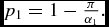 $p_{1}=1-\frac{\pi }{\alpha _{1}}.$
The question now is whether such steady states exist. To explore this question, recall that rH(m) and rS(m) denote respectively, for any m, the rental rate at which healthy individuals in the high-prevalence city are just deterred from migrating to the low prevalence city, and the rental rate at which sick individuals in the low-prevalence city can just be induced to migrate to the high-prevalence city. It is evident that rH(m) is decreasing in m and rS(m) is increasing in m. Let m* be the value of m such that rH(m*) = rS(m*).
Figure 1 illustrates as follows: It shows rH(m) and rS(m), which will cross at a strictly positive value of m, which we have defined as m*, provided that rH(0) > rS(0).Footnote 16
Combinations of migration costs and rental rates leading sick and healthy individuals to be indifferent about migration.

Appendix shows that rH(0) > rS(0), such that we can establish the following Proposition:
Proposition 4 There exists m* > 0 such that, for all m < m*, an equilibrium exists with 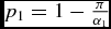 $p_{1}=1-\frac{\pi }{\alpha _{1}}$ and p 2 = 0. In this equilibrium, there is non-zero gross migration outside the steady state but not at the steady state.
The intuition behind the proof is relatively straightforward: because the healthy are more willing than the sick to pay to live in the low-prevalence city, there will be a rental rate that compensates the sick for moving to the high-prevalence city and does not deter the healthy from migrating to the low-prevalence city, provided migration costs are low enough.
Note how the possibility of migration out of the steady state makes the crucial difference between the steady states described in Propositions 3 and 4 even though in the steady state no actual migration takes place. This is because any infected individuals who arise in city 2, instead of remaining in city 2 where they progressively infect the rest of the population, migrate out immediately to city 1. This keeps the prevalence rate at zero in city 2. It has no lasting effect on the prevalence in city 1, though, because in the steady state there is no further in-migration and the prevalence in city 1 is determined in exactly the same way as it was in the non-migration steady state.
Moreover, we show in the Appendix that the Low migration costs characterized above generate an unstable root, which pushes the prevalence rate in the healthy city to a corner. This type of corner steady state is the only one compatible with positive migration flows along the transition path and is robust to small changes of parameter values.
It is straightforward to show that there is no steady state equilibrium with non-zero gross migration in steady state (such that ϕ > 0, ψ > 0 ), because to do so would require the two migration inequalities (13) and (14) to bind at the same level of r, which is impossible as shown in the proof of Proposition 1.Footnote 17
Having established the existence of these equilibria, we now turn to highlighting an interesting property of the steady state with migration in Proposition 5.
Proposition 5 In the equilibrium with p 2 = 0, the healthy city may be the city with the more disease-prone environment, that is,  $p_{2}<p_{1\text{ }}$is compatible with α2 > α1.
The proof of this proposition follows immediately from Proposition 1 and noting that if p 2 = 0, α2p 2 = 0 < α1p 1 whatever the value of α2.
This shows that, in the case of Low migration costs, there is a possibility of multiple equilibria because of strategic complementarities in the utility function. Indeed the probability of becoming infected is a positive function of the degree of disease-proneness in city i, αi, and of the proportion of sick individuals in city i, pi, but the latter is determined in equilibrium. This generates a clear coordination problem and underlines an important role of expectations in the model. A city can be established as the more healthy city, and therefore become a destination for healthy individuals, with higher rents that drive out sick individuals, simply because it is expected to be more healthy, in spite of having a more disease-prone environment. However, it is unlikely that it would become so established if migration costs are initially very high and are gradually reduced, since the autarky prevalence of the more disease-prone city will be higher, so that initial migration by the healthy is likely to be from the more disease-prone to the less disease-prone environment.
Finally, we can show that the range of values of m for which a steady state exists with migration by the healthy to the city with the more disease-prone environment is strictly smaller than the range of values of m for which a steady state exists with migration by the healthy to the city with the less disease-prone environment. A consequence of the proof of Proposition 4 is that rH(0) − rS(0) is strictly decreasing in the value of α2 as well as in the value of π. Thus, the more disease prone the environment of the city to which the healthy are migrating and the higher the recovery rate, the smaller the value of the m* for which a migration equilibrium exists. This is rather intuitive since a more disease prone environment of the healthy city and a higher recovery rate make migration less attractive as a way of escaping from endemic diseases.
This allows us to state our final proposition which characterizes existence conditions of steady state equilibria for all values of m.
Proposition 6 For any value of π, there exists two strictly positive values of m, m*, and m′, with m′ < m* such that, the following steady state equilibria exist:
1) when migration costs exceed m*, there is no migration;
 $p_{1}=1- \frac{\pi }{\alpha _{1}}$ and $p_{2}=1-\frac{\pi }{\alpha _{2}}$.
2) when migration costs lie between m′ and m*, the only equilibrium has migration out of steady state by the healthy from the city with the more disease-prone environment to the city with the less disease-prone environment;
$p_{1}=1-\frac{\pi }{\alpha _{1}}$ and p 2 = 0.3) when migration costs lie below m′, there are two steady state equilibria in each of which
$p_{1}=1-\frac{\pi }{\alpha _{1}}$ and p 2 = 0 . In the first steady state, city 2, the city to which the healthy migrate out of steady state, is the one with the less disease-prone environment and, in the second, city 2 is the one with the more disease-prone environment.
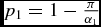
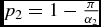
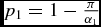
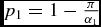
Figure 2 illustrates the relation of m′ to m*.
Thresholds for existence and multiplicity of steady state equilibria.
5.3. Welfare Comparisons
Now, we can consider the comparative welfare properties of the steady states with and without the possibility of migration. It is straightforward to see that the steady states with migration are Pareto-superior to the steady state without migration. Prevalence in city 1 is the same in the steady states defined by Propositions 3 and 4; only that in city 2 differs (and is strictly lower in the migration steady states). Given that there is no migration (and therefore no migration costs incurred) in all steady states, this means that the steady states with migration have fewer sick individuals and incur no offsetting costs. We have therefore established the following:
Proposition 7 The steady states with migration are Pareto-Superior to the steady state without migration.
However, we can also Pareto-rank the two steady states that exist when migration costs lie below m′, since they differ in their values of α1, and therefore in the prevalence rates in the high-prevalence city. It is immediate that
Proposition 8 The second steady state, that exists only when migration costs are lower than m′, has lower prevalence than, and is therefore Pareto Superior to, the first steady state.
Proposition 6 has merely characterized the steady states according to whether or not migration costs are low enough for gross migration to occur out of steady state. The fact that the steady states with non-zero gross migration out of equilibrium Pareto-dominate that with zero migration has important implications for policy. In this model, it is a good thing for there to be outmigration of sick individuals from city 2 (driven by the higher rents due to competition from individuals in-migrating from city 1 ). The reason for this is that outmigration of such individuals removes them from where they would contribute to new infections and places them in a city in which the disease is already established and to which their presence will bring no lasting deterioration in the prevalence. In these circumstances, action by the authorities should not be to discourage migration (which may be a by-product of quarantine measure or of other types of migration restrictions) but rather actively to encourage it. In the steady state, there will in fact be no migration, but out of the steady state such migration is an important means of reducing the risk that the disease established in city 1 also establishes itself in city 2.
6. CONCLUSION
Our analysis indicates that differences in disease prevalence rates can emerge as the equilibrium outcome of more fundamental differences in environment, with migration behavior acting as a means of arbitrage between locations with different prevalence levels. We have also shown that whether migration takes place out of the steady state has important implications for steady state prevalence levels even if there is no migration at the steady state. In particular, it is desirable for infected individuals to migrate away from low-prevalence localities since these are the ones in which they create the greatest negative externalities. This has potentially important implications for policy since it suggests that, far from seeking to discourage voluntary migration in conditions of endemic disease, it may sometimes be desirable to encourage it.
A key mechanism in our model is that the willingness to pay of healthy individuals to live close to other healthy individuals exceeds that of sick individuals, which leads to sorting by health and higher costs of living in healthier areas. This, however, is true only under certain conditions. As we discussed, under certain alternative assumptions, it could be that sick individuals would have a higher willingness to pay to live in low-prevalence environments, which would act against segregation: recovery rates may, for example, be higher in rich cities due to better health infrastructures and income dynamics or family decisions may make sick people less likely to migrate to poor cities with high prevalence rates. Moreover, as highlighted in Mesnard and Seabright (Reference Mesnard and Seabright2009), under different assumptions about the distribution of past exposure to the disease and the asymmetric information individuals may have on their own risk, migrants to low-prevalence destinations may include a significant proportion of asymptomatic individuals likely to become sick, thereby mitigating segregation effects in the short run even if they do not wholly offset them.
Finally, we have shown that expectations may matter in this model with fully rational individuals, which leads to the possibility of multiple equilibria and generates an interesting coordination problem. However, it is also possible that individuals are not fully rational nor perfectly informed on their health risks when considering their location decisions, which may lead to the existence of other equilibria.
The conditions described in our model are thus not general but they do constitute an important class of cases for public policy to bear in mind. They warn policy makers to take into account positive externalities generated by migration in the presence of endemic diseases. Public policy needs to model very carefully the interactions between disease and migration in order to ensure that policy interventions do not have counter-productive consequences in the short run (Mesnard and Seabright Reference Mesnard and Seabright2009) and in the long run, as highlighted in the present paper. We also believe that segregation by disease-prevalence of neighborhoods within cities, and of regions within countries, has been a phenomenon of historical significance which models of this kind can help us to understand. Given the startling differences in disease prevalence between different regions of the world, it remains of real significance today. And given the likely emergence of new forms of antibiotic-resistant infections in years to come, some of which may become endemic in certain parts of the world, the problem can only grow in importance in the future.
APPENDIX A: PROOFS
Lemma 1 There cannot be migration in both directions in equilibrium by individuals of a given type.
Proof of Lemma 1.
The proof is by contradiction. Suppose that if rt = rHt(m), inequality (13) is weakly satisfied for i = 2.
Then, inserting rHt(m) in inequality (13) for i = 1 yields
 $$\begin{equation}
U\left( Y,H\right) -U\left( Y-r_{t}^{H}(m),H\right) =Z_{t}-m,
\end{equation}$$
where
 $$\begin{eqnarray*}
Z_{t}&=&\gamma \alpha _{2}p_{2t}W_{2t+1}(S)-\gamma \alpha _{1}p_{1t}W_{1t+1}(S)\\
&&+\,\gamma (1-\alpha _{2}p_{2t})W_{2t+1}(H)-\gamma (1-\alpha _{1}p_{1t})W_{1t+1}(H).
\end{eqnarray*}$$
Setting i = 2 in inequality (13) yields
 $$\begin{equation*}
0\le U\left( Y,H\right) -U\left( Y-r_{t}^{H}(m),H\right) -m-Z_{t}
\end{equation*}$$
and substituting equation (22) in inequality (13) yields
 $$\begin{equation*}
0\le Z_{t}-m-m-Z_{t}
\end{equation*}$$
which is a contradiction as m > 0. This shows that inequality (13) cannot be satisfied for both i = 1 and i = 2 if rt = rHt(m). For all rt > rHt(m), inequality (13) will not be satisfied for i = 1, while for all rt < rHt(m) inequality (13) will not be satisfied for i = 2. Thus, inequality (13) cannot be simultaneously satisfied for i = 1 and i = 2 at any value of rt. Analogous arguments when inequality (14) binds for i = 2 inequality (14) cannot be simultaneously satisfied for i = 1 and i = 2 at any value of rt. ▪
Lemma 2 establishes that an equilibrium exists:
Lemma 2 For any p 1t, p 2tand for any s 1t, s 2timplied by p 1t, p 2t, there exist hit, for i = 1, 2 such that equation (16) is satisfied with0 ⩽ hit ⩽ 1.
Proof of Lemma 2.
From Lemma 1, we know that if sit > 0, sjt = 0 and that if hit > 0 , hjt = 0. Thus, equation (16) implies
 $$\begin{equation*}
s_{it}p_{it}=h_{jt}\left( 1-p_{jt}\right) \text{ for }i=1,2
\end{equation*}$$
which can be rewritten
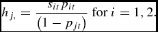 $$\begin{equation*}
h_{j,}=\frac{s_{it}p_{it}}{\left( 1-p_{jt}\right) }\text{ for }i=1,2.
\end{equation*}$$
Since equation (1) implies that 0 ⩽ pit < (1 − pjt) and since 0 ⩽ sit ⩽ 1, it follows that 0 ⩽ hit ⩽ 1. ▪
Properties of Steady State Equilibria
We write Wi(H) = Wit(H) = W it + 1(H) and Wi(S) = Wit(S) = W it + 1(S) for the continuation value of living in city i for a healthy and a sick individual respectively.
We can therefore write the migration conditions (13) and (14) in their steady state forms as
 $$\begin{eqnarray}
0 &\le &U\left( Y-r_{j},H\right) -U\left( Y-r_{i},H\right) -m+\gamma \alpha _{j}p_{j}W_{j}(S)-\gamma \alpha _{i}p_{i}W_{i}(S) \nonumber \\
&&+\gamma (1-\alpha _{j}p_{j})W_{j}(H)-\gamma (1-\alpha _{i}p_{i})W_{i}(H)
\end{eqnarray}$$
and
 $$\begin{eqnarray}
0 &\le &U\left( Y-r_{j},S\right) -U\left( Y-r_{i},S\right) -m+\gamma \pi \left( W_{j}\left( H\right) -W_{i}\left( H\right) \right) \nonumber \\
&&+\gamma \left( 1-\pi \right) \left( W_{j}\left( S\right) -W_{i}\left( S\right) \right).
\end{eqnarray}$$
We can then show two properties of the continuation values summarized in Lemmas 3 and 4.
Lemma 3 In steady state equilibrium, the additional continuation value of being healthy rather than sick in city i, Wi(H) − Wi(S), is strictly positive and decreasing in the prevalence rate pi, in the unhealthiness parameter αi, and in the recovery rate π.
Proof. Subtracting equation (11) from equation (9) yields
 $$\begin{eqnarray*}
W^{i}\left( H\right) -W^{i}\left( S\right) &=&U\left( Y-r_{i},H\right) -U\left( Y-r_{i},S\right) \\
&&+\gamma (1-\alpha _{i}p_{i}-\pi )W^{i}\left( H\right) -\gamma (1-\alpha _{i}p_{i}-\pi )W^{i}\left( S\right)
\end{eqnarray*}$$
which implies that
 $$\begin{equation*}
W^{i}\left( H\right) -W^{i}\left( S\right) =\frac{U\left( Y-r_{i},H\right) -U\left( Y-r_{i},S\right) }{1-\gamma (1-\alpha _{i}p_{i}-\pi )}
\end{equation*}$$
which is strictly positive by assumption (6) and strictly decreasing in αi, pi, and π. ▪
Lemma 4 In steady state equilibrium, if αjpj > αipi the difference between the additional continuation values for healthy and sick individuals of living in city i rather than in city j, (Wi(H) − Wj(H)) − (Wi(S) − Wj(S)), is str ictly positive and decreasing in the prevalence rate pi, in the unhealthiness parameter αi, and in the recovery rate π.
Proof.
From equation (9) we can write
 $$\begin{eqnarray}
W^{i}\left( H\right) -W^{j}\left( H\right) &=&U\left( Y-r_{i},H\right) -U\left( Y-r_{j},H\right) +\gamma \alpha _{i}p_{i}W^{i}\left( S\right) -\gamma \alpha _{j}p_{j}W^{j}\left( S\right) \nonumber \\
&&+\gamma \left( 1-\alpha _{i}p_{i}\right) W^{i}\left( H\right) -\gamma \left( 1-\alpha _{j}p_{j}\right) W^{j}\left( H\right).
\end{eqnarray}$$
Similarly,
 $$\begin{eqnarray}
W^{i}\left( S\right) -W^{j}\left( S\right) &=&U\left( Y-r_{i},S\right) -U\left( Y-r_{j},S\right) +\gamma \pi \left[ W^{i}\left( H\right) -W^{j}\left( H\right) \right] \nonumber \\
&&+\gamma \left( 1-\pi \right) \left[ W^{i}\left( S\right) -W^{j}\left( S\right) \right].
\end{eqnarray}$$
First, note that U(Y − ri, θ) − U(Y − rj, θ) is independent of θ by equation (8), thus [U(Y − ri, H) − U(Y − rj, H)] − [U(Y − ri, S) − U(Y − rj, S)] = 0.
Therefore, subtracting equation (26) from equation (25) and re-arranging yields
 $$\begin{eqnarray*}
&&W^{i}\left( H\right) -W^{j}\left( H\right) -\left[ W^{i}\left( S\right) -W^{j}\left( S\right) \right] \\
&&\quad =W^{i}\left( H\right) \left[ \gamma (1-\alpha _{i}p_{i}-\pi )\right] -W^{i}\left( S\right) \left[ \gamma (1-\alpha _{i}p_{i}-\pi )\right] \\
&&\qquad \ldots -W^{j}\left( H\right) \left[ \gamma (1-\alpha _{j}p_{j}-\pi )\right] +W^{j}\left( S\right) \left[ \gamma (1-\alpha _{j}p_{j}-\pi )\right]
\end{eqnarray*}$$
which in turn yields
 $$\begin{eqnarray*}
&&W^{i}\left( H\right) -W^{j}\left( H\right) -W^{i}\left( S\right) +W^{j}\left( S\right) \\
&&\quad =\frac{1}{1-\gamma (1-\pi )}\left[ \alpha _{j}p_{j}\left( W^{j}\left( H\right) -W^{j}\left( S\right) \right) -\alpha _{i}p_{i}\left( W^{i}\left( H\right) -W^{i}\left( S\right) \right) \right].
\end{eqnarray*}$$
The RHS expression is strictly positive because αjpj > αipi and
 $$\begin{equation*}
\alpha _{i}p_{i}\left( W^{i}\left( H\right) -W^{i}\left( S\right) \right) =\alpha _{i}p_{i}\frac{U\left( Y-r_{i},H\right) -U\left( Y-r_{i},S\right) }{ 1-\gamma (1-\alpha _{i}p_{i}-\pi )}
\end{equation*}$$
which is strictly increasing in αipi because  $\frac{x}{1+c+bx}$ is strictly increasing in x for all x if 1 + c ⩾ 0. ▪
Proof of Proposition 1.
Define r*(S) as the value of r 2 such that inequality (24) binds for i = 1. Intuitively, r*(S) is the value of rental in the low-prevalence city that is just high enough to dissuade sick individuals from moving there from the high-prevalence city. This yields
 $$\begin{equation}
U\left( Y,S\right) -U\left( Y-r^{\ast }(S),S\right) =Z^{^{\prime }}-m,
\end{equation}$$
where
 $$\begin{equation*}
Z^{^{\prime }}=\gamma \pi \left( W^{2}\left( H\right) -W^{1}\left( H\right) \right) +\gamma \left( 1-\pi \right) \left( W^{2}\left( S\right) -W^{1}\left( S\right) \right).
\end{equation*}$$
Substracting Z ′ from Z yields
 $$\begin{eqnarray*}
Z-Z^{^{\prime }} &=&W^{2}(H)\left[ \gamma (1-\alpha _{2}p_{2}-\pi )\right] -W^{1}(H)\left[ \gamma (1-\alpha _{1}p_{1}-\pi )\right] \\
&&+W^{2}(S)\left[ \gamma \left( \alpha _{2}p_{2}+\pi -1\right) \right] -W^{1}(S)\left[ \gamma \left( \alpha _{1}p_{1}+\pi -1\right) \right].
\end{eqnarray*}$$
Simplifying yields
 $$\begin{equation*}
Z-Z^{^{\prime }}=\gamma (1-\alpha _{2}p_{2}-\pi )\left[ W^{2}(H)-W^{2}(S) \right] -\gamma (1-\alpha _{1}p_{1}-\pi )\left[ W^{1}(H)-W^{1}(S)\right].
\end{equation*}$$
This must be strictly greater than zero since (1 − α2p 2 − π) > (1 − α1p 1 − π) and W 2(H) − W 1(H) ⩾ W 2(S) − W 1(S) from Lemma 4. Therefore, from equations (22) and (27) we can see that
 $$\begin{equation*}
U\left( Y,H\right) -U\left( Y-r^{\ast }(H),H\right) >U\left( Y,S\right) -U\left( Y-r^{\ast }(S),S\right)
\end{equation*}$$
which implies that r*(H) > r*(S) given equation (8). Thus, sick individuals will be dissuaded from migrating to the low-prevalence city at a lower rental rate than will dissuade healthy individuals. Thus, for any rental rate at which sick individuals want to migrate to the low-prevalence city, healthy individuals also want to migrate in this direction. Since by Lemma 1, there cannot be individuals of either health status simultaneously wishing to migrate in the opposite direction, this cannot be an equilibrium satisfying the zero net migration condition. Thus, in equilibrium sick individuals, if they migrate at all in equilibrium, must migrate only to the high-prevalence city. Analogous arguments show that sick individuals will choose to migrate from the high-prevalence city at a lower rental rate than healthy individuals.
Therefore, there is no rental rate at which only sick individuals migrate to the low-prevalence city and healthy individuals to the high-prevalence city. Thus, healthy individuals, if they migrate, will do so from the high-prevalence to the low-prevalence city while sick individuals, if they migrate, will do so in the opposite direction. ▪
Proof of Proposition 4.
Using equation (13), we define rHt(m) implicitly as follows:
 $$\begin{eqnarray}
m &=&U\left( Y-r_{t}^{H}(m),H\right) -U\left( Y,H\right) +\gamma \alpha _{j}p_{jt}W_{jt+1}(S)-\gamma \alpha _{i}p_{it}W_{it+1}(S) \nonumber \\
&&+\gamma (1-\alpha _{j}p_{jt})W_{jt+1}(H)-\gamma (1-\alpha _{i}p_{it})W_{it+1}(H).
\end{eqnarray}$$
Substituting i = 1 and j = 2, taking steady state values and noting that 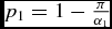 $p_{1}=1-\frac{\pi }{\alpha _{1}}$ and p 2 = 0 yields
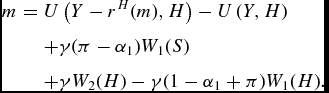 $$\begin{eqnarray}
m &=&U\left( Y-r^{H}(m),H\right) -U\left( Y,H\right) \nonumber \\
&&+\gamma (\pi -\alpha _{1})W_{1}(S) \nonumber \\
&&+\gamma W_{2}(H)-\gamma (1-\alpha _{1}+\pi )W_{1}(H).
\end{eqnarray}$$
Using equation (14), we define rSt(m) implicitly as follows:
 $$\begin{eqnarray}
m &=&U\left( Y,S\right) -U\left( Y-r_{t}^{S}(m),S\right) +\gamma \pi \left( W_{jt+1}\left( H\right) -W_{it+1}\left( H\right) \right) \nonumber \\
&&+\gamma \left( 1-\pi \right) \left( W_{jt+1}\left( S\right) -W_{it+1}\left( S\right) \right).
\end{eqnarray}$$
Substituting i = 2 and j = 1, taking steady state values and noting that 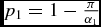 $p_{1}=1-\frac{\pi }{\alpha _{1}}$ and p 2 = 0 yields
 $$\begin{eqnarray}
m &=&U\left( Y,S\right) -U\left( Y-r^{S}(m),S\right) +\gamma \pi \left( W_{1}\left( H\right) -W_{2}\left( H\right) \right) \nonumber \\
&&+\gamma \left( 1-\pi \right) \left( W_{1}\left( S\right) -W_{2}\left( S\right) \right).
\end{eqnarray}$$
Equation (8) implies that rH(0) > rS(0) if U(Y, H) − U(Y − rH(0), H) > U(Y, S) − U(Y − rS(0), S).
Define R ≡ (U(Y, H) − U(Y − rH(0), H)) − (U(Y, S) − U(Y − rS(0), S)). Then, setting m = 0 and using equations (29) and (31) yields
 $$\begin{eqnarray}
R &=&\gamma W_{2}(H)-\gamma (1-\alpha _{1}+\pi )W_{1}(H)+\gamma (\pi -\alpha _{1})W_{1}(S) \nonumber \\
&&+\gamma \pi \left( W_{1}\left( H\right) -W_{2}\left( H\right) \right) +\gamma \left( 1-\pi \right) \left( W_{1}\left( S\right) -W_{2}\left( S\right) \right).
\end{eqnarray}$$
This can be rewritten as R = Aγ(1 − π) + B(α1 − π), where
 $$\begin{equation*}
A=\left( W_{2}\left( H\right) -W_{1}\left( H\right) \right) -\left( W_{2}\left( S\right) -W_{1}\left( S\right) \right)
\end{equation*}$$
which, since α1p 1 > α2p 2, is strictly positive by Lemma 4, and
 $$\begin{equation*}
B=\left( W_{1}\left( H\right) -W_{1}\left( S\right) \right)
\end{equation*}$$
which is strictly positive by Lemma 3. Therefore, R > 0, which implies that rH(0) > rS(0).
Using the definition of m* this implies that m* > 0.
Lemmas 3 and 4 also imply that R, and therefore rH(0) − rS(0), is decreasing in α2 and in π. ▪
APPENDIX B
Local Stability of the Equilibrium without Migration
 $$\begin{equation*}
p_{it+1}=u(p_{it})=\alpha _{i}p_{it}(1-p_{it})+p_{it}(1-\pi ).
\end{equation*}$$
The steady state equilibrium in each city is a fixed point such that u′(pi) = pi.
We can derive the function u(.) as u′(pit) = 1 − π + αi − 2αipit and note that the steady state pi is stable if |u′(pit)| < 1 around the steady state.
This condition is equivalent to
 $$\begin{equation*}
2(\alpha _{i}p_{it}-1)<-\pi +\alpha _{i}<2\alpha _{i}p_{it}.
\end{equation*}$$
We can show easily that 2(αipit − 1) < −π + αi since − π + αi > 0 by assumption and αipit < 1.
Since pi = 1 − π/αi for i = 1, 2 we show easily that, close to the steady state, 2αipit≅2(αi − π), which is clearly larger than αi − π.
Therefore, the steady state equilibrium is locally stable.
Local Stability of the Equilibria with Migration
We have the following dynamic system:
 $$\begin{eqnarray*}
p_{1t+1} &=&f(p_{1t},p_{2t})=\left[ (1-p_{1t})(1-h_{1t})\alpha _{1}+(1-\pi ) \right] p_{1t}+s_{2t}p_{2t}(1-\pi ); \\
p_{2t+1} &=&g(p_{1t},p_{2t})=h_{1t}(1-p_{1t})\alpha _{2}p_{2t}+\alpha _{2}p_{2t}(1-p_{2t})+(1-s_{2t})p_{2,}(1-\pi ).
\end{eqnarray*}$$
We note
 $$\begin{equation*}
J=\left(\begin{array}{cc}(1-\pi )-(1-h_{1t})\alpha _{1}p_{1t}+(1-h_{1t})\alpha _{1} & s_{2t}(1-\pi ) \\
-h_{1t}\alpha _{2}p_{2t} & \alpha _{2}-\alpha _{2}p_{2t}+h_{1t}(1-p_{1t})\alpha _{2}+(1-s_{2t})(1-\pi ) \end{array}\right).
\end{equation*}$$
After writing  $p(\chi )=\left|J-\chi I\right|=|\scriptsize\begin{array}{cc}f_{p_{1}}-\chi & f_{p_{2}} \\
g_{p_{1}} & g_{p_{2}}-\chi \end{array} |$, we can study the Eigenvalues of J, roots of the equation p(χ) ≡ χ2 − (tr
 $J)\chi +\det J=0.$
We know that in Equilibrium s 2(=φ) = h 1(=ψ) = 0, p 1 = 1 − π/α1, and p 2 = 0 such that 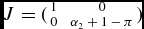 $J=(\scriptsize\begin{array}{c@c}1 & 0 \\
0 & \alpha _{2}+1-\pi \end{array})$ and p(χ) can be rewritten as
 $$\begin{equation*}
p(\chi )=\chi ^{2}-(2-\pi +\alpha _{2})\chi +(\alpha _{2}+1-\pi ).
\end{equation*}$$
The two Eigenvalues χ1 and χ2 are as follows:
 $$\begin{eqnarray*}
\chi _{1} &=&\alpha _{2}-\pi +1; \\
\chi _{2} &=&1.
\end{eqnarray*}$$
Since |χ1| > 1 and |χ2| = 1 such equilibria are locally unstable.




