1. Introduction
The scramjet is a key technology in supersonic and hypersonic aircraft research due to its superior thrust performance (Hank, Murphy & Mutzman Reference Hank, Murphy and Mutzman2008). Scramjet engine typically comprises four main components: supersonic intake (Shi et al. Reference Shi, Chang, Ma, Wang, Gao and Bao2019), isolator (Xiong et al. Reference Xiong, Fan, Wang, Zhou and Tao2017a ; Wang et al. Reference Wang, Huang, Li, Zheng, Guo and Chang2023), combustor (Lv et al. Reference Lv, Xia, Liu and Huang2017) and nozzle (Ijas Muhammed et al. Reference Ijas Muhammed, Shamsia Banu, Suryan, Lijo, Simurda and Kim2024). At supersonic speeds, the internal flow field within the scramjet becomes highly unstable, which can significantly impact the safety and operational stability of the aircraft. The isolator plays a crucial role in mitigating these instabilities. It prevents the interaction between multiple shock waves generated in the intake and the unsteady, pulsating combustion occurring in the combustor. By doing so, it inhibits the transmission of pressure oscillations from the downstream combustor to the upstream intake, thereby reducing the risk of inlet unstart and ensuring safer engine operation (Huang et al. Reference Huang, Wang, Pourkashanian, Ma, Ingham, Luo and Lei2011; Tan et al. Reference Tan, Li, Wen and Zhang2011; Idris et al. Reference Idris, Saad, Zare-Behtash and Kontis2014). Moreover, the isolator facilitates flow deceleration and pressurisation through complex internal dynamics, supplying the combustor with higher pressure and relatively lower-speed airflow compared with the intake (Wagner et al. Reference Wagner, Yuceil, Valdivia, Clemens and Dolling2009). It not only enhances combustion efficiency, but also contributes to improved overall thrust performance of the scramjet engine.
The supersonic flow within the duct passes through a pseudo-shock wave (PSW) structure that includes both the shock train and a downstream mixing region, as demonstrated in figure 1. During this process, multiple shock waves, expansion fans and boundary layer separations can be observed (Gnani, Zare-Behtash & Kontis Reference Gnani, Zare-Behtash and Kontis2016). The incoming supersonic flow generates multiple shock waves within the duct and the interaction between these shock waves and the boundary layer, which is known as the shock wave/boundary layer interaction (SWBLI), further complicates the flow field. Matsuo, Miyazato & Kim (Reference Matsuo, Miyazato and Kim1999) proposed a classification of shock wave modes based on the interaction between normal shock waves and turbulent boundary layers. When the Mach number is below 1.2, a normal shock wave similar to an inviscid normal shock wave is formed within the duct. For Mach numbers between 1.2 and 1.3, the shock becomes slightly curved with minimal boundary layer separation. In the range of Mach 1.3–1.5, increased separation of the boundary layer causes the shock wave to form the ‘λ’ foot structure. At Mach number above 1.5, a multiple shock wave system is formed in the duct, which is termed a shock train. If the duct is sufficiently long, then the flow reaches the mixing region where the high momentum core flow mixes with low momentum boundary layer flow. As the inlet Mach number increases, the shock wave pattern transforms from the normal shock to the oblique shock pattern.
The unsteady motion of shock trains can be roughly divided into self-excited oscillation and forced oscillation. In addition to these, factors such as duct resonance, boundary layer separation behind shocks and the presence of turbulent fluctuations make the actual oscillation spectrum distribution extremely complex. Summarising previous research findings, studies on shock train oscillations in isolators have mainly focused on the geometric shape of the isolator (Wang et al. Reference Wang, Tian, Cheng and Wu2008) and boundary conditions such as the incoming Mach number (Hou et al. Reference Hou, Chang, Kong, Bao and Dala2020), wall temperature gradients (Mahmood et al. Reference Mahmood, Kamali, Sotoudeh, Karimi and Khojasteh2021), and the pressure ratio between the upstream and downstream of the duct (Sethuraman, Kim & Kim Reference Sethuraman, Kim and Kim2020).
Schematic of the PSW.

Self-excited oscillation is an unsteady phenomenon associated with a shock train, characterised by spontaneous movement of the shock system without any change in the initial boundary condition. This behaviour reflects the inherently unsteady feature of the shock train. Such self-excited oscillation has been observed in various components of the scramjet engine (Chen, Gao & Liang Reference Chen, Gao and Liang2019; James, Suryan & Kim Reference James, Suryan and Kim2021; Wu et al. Reference Wu, Fan, Fu, Kumar and Sethuraman2024). When the supersonic flow enters the isolator, periodic fluctuations are induced by self-excited oscillation in flow parameters, which can significantly impact the isolator’s stability and compromise the overall safety of the scramjet operation. Deng et al. (Reference Deng, Wu, Kim and Chen2023) conducted a numerical study on the relationship between the self-excited oscillation of the shock train and the isolator length. They found that the length of the shock train increases with the increase in the isolator length; under this condition, the leading shock tends to be stable, while the subsequent shocks show an opposite variation trend. James, Sethuraman & Kim (Reference James, Sethuraman and Kim2023) conducted numerical studies on the duct length downstream of the isolator to analyse the influence of duct acoustics on the dynamics of shock train self-excited oscillation. Their results demonstrated, through narrow-band time delay analysis, that disturbances induced by flow separation can propagate upstream and downstream within the shock train region. As the duct length increases, the velocity of the downstream disturbances decreases, indicating that the resonance effect within the duct influences the characteristics of the self-excited oscillation. Xiong et al. (Reference Xiong, Wang, Fan and Wang2017b ; Reference Xiong, Fan, Wang and Tao2018) experimentally detected self-excited oscillations of the shock train at M a = 3, characterised by low-frequency oscillations below 200 Hz. They ascribed this behaviour to the driving effect of separation shock motions, with the separation bubble enhancing disturbance frequencies. Ikui et al. (Reference Ikui, Matsuo, Nagai and Honjo1974) noted that a rise in the incoming flow Mach number leads to enhanced self-excited oscillations of the shock train, and they ascribed this trend to the interplay between minor upstream disturbances and the shock waves. Hou et al. (Reference Hou, Chang, Kong, Bao and Dala2020) studied shock train self-excited oscillation in an isolator with a background wave system via wind tunnel tests. They found discontinuous pressure pulsations from the background wave system severely affected shock train asymmetry and unstable separation near the shock train leading edge (STLE) interfered with oscillation. Sethuraman, Yang & Kim (Reference Sethuraman, Yang and Kim2022) carried out numerical simulations on the self-excited oscillation of shock trains under boundary layer suction conditions. Through comparative analysis of three inclined suction slots with different suction flow ratios in a constant area duct, it was confirmed that the length of the shock train would be significantly shortened compared with the condition without suction, and the curve of power spectral density showed that the length of the shock train would be reduced significantly. The dominant frequency increases with the increase of the suction ratio. Wang, Xiong & Fan (Reference Wang, Xiong and Fan2021, Reference Wang, Chang, Hou and Yu2020) conducted wind tunnel tests combined with coherence and phase analysis to reveal the kinematic correlation between various shock waves in the isolator and identify Type III oscillations, which are independent shock wave motion processes. Their research results showed that downstream disturbances first trigger the movement of the STLE, and the closer the downstream shock wave is to the STLE, the faster the response. Additionally, the greater the number of shock waves in the shock train, the more frequent the reflections, which in turn reduces the overall coherence of the system.
In addition to self-excited oscillation, forced oscillation represents another key unsteady phenomenon: it describes shock train oscillation driven by variable disturbances in external boundary conditions, and its excitation sources are disturbances from the unsteady operation of the inlet and combustor. Regarding studies on the effect of upstream disturbances on the forced oscillation of shock trains, James & Kim (Reference James and Kim2023) conducted numerical research and found that a larger amplitude of upstream disturbances causes the probability density function (p.d.f.) of shock location to deviate notably from a Gaussian distribution, with a concurrent rise in the root mean square (r.m.s.) of the oscillation amplitude. Gnani et al. (Reference Gnani, Zare-Behtash, White and Kontis2018a ) and Sethuraman, Kim & Kim (Reference Sethuraman, Kim and Kim2021) analysed the forced oscillations of the shock train caused by backpressure disturbances in a rectangular isolator with a Mach number of 1.75. Their results indicated that the peak frequency of self-excited oscillation decreased while the peak value of the power spectrum value increased linearly with the increase of disturbance amplitude. In addition, Deng, Kim & Chen (Reference Deng, Kim and Chen2020) also found that the amplitude of the forced oscillation of the shock train driven by backpressure disturbances is inversely proportional to the driving frequency. Li (Reference Li2022) used URANS simulations to investigate how the fluctuating amplitude and frequency of the incoming flow angle of attack affect shock train dynamics. The results showed that the shock train’s oscillation amplitude does not rise monotonically with the excitation amplitude; certain excitation amplitudes can enhance pressure peaks in the SWBLI region, thus effectively inhibiting the upstream movement of the separation shock. Once the excitation amplitude surpasses a critical threshold, however, the shock train’s oscillation region expands substantially, along with heightened pressure fluctuations.
To evaluate the differences in oscillation between the normal shock train and the oblique shock train, Wang et al. (Reference Wang, Chang, Wu and Yu2021) conducted experiments in a rectangular duct with Mach numbers 2 and 3. By mechanically adjusting the throttling ratio, the shock train was forced to oscillate under different backpressure ratios. The results display that the forced oscillation of the shock train with Mach number 3 is more obvious and is a compound mode, which is the coupling of the excitation frequency and the natural pulsation frequency. In addition, a frequency correlation was observed between the wall pressure and the downstream excitation. Many other scholars have also conducted research on the propagation mechanism of disturbances under forced oscillations and it is now generally recognised that the spread of downstream disturbances triggers oscillations of the leading shock. This shock subsequently produces perturbations that travel downstream and influence the oscillations of other shocks (Yamane et al. Reference Yamane, Kondo, Tomita and Sakae1984). The propagation speeds of disturbances in the flow field show a negative correlation with the frequencies of backpressure disturbances (Sethuraman et al. Reference Sethuraman, Kim and Kim2021).
Separating the research on self-excited oscillations and forced oscillations helps simplify complex multi-modal oscillations, thereby obtaining conclusions with stronger pertinence. The pressure ratio at the inlet and outlet of the isolator is a direct factor affecting the STLE; therefore, this study uses this single independent variable to investigate the self-excited oscillation of the shock train. For forced oscillations, this study sets pressure fluctuation functions upstream and downstream of the model to simulate disturbance sources. Although the current research approach has been reflected in previous studies, the innovation of this paper lies in the adoption of a three-dimensional (3-D) rectangular diverging isolator and the use of large-eddy simulation (LES) (Lee et al. Reference Lee, Wantanabe, Kouchi and Masuya2012; Quaatz et al. Reference Quaatz, Giglmaier, Hickel and Adams2014) as the numerical simulation method. Previous two-dimensional (2-D) models ignored the 3-D effects in actual engineering and led to inaccuracies in boundary layer thickness (Gnani et al. Reference Gnani, Zare-Behtash, White and Kontis2018b ).
Previous experimental and computational studies have revealed the multi-shock structure and low-frequency breathing of shock trains, yet most analyses report only time-averaged or short excerpts, leaving the phase-resolved dynamics and input–output response under-characterised. Furthermore, several forcing studies employed reflective outlets or limited durations, complicating the distinction between true suppression and boundary-feedback artefacts. Existing high-speed LES typically emphasise shock robustness through AUSM+/Roe/WENO schemes but seldom document spectral adequacy, wall-resolution metrics (y +, Δx +, Δz +) or scheme sensitivity. In this context, the present work applies LES with AUSM+ flux splitting, full near-wall and anisotropy metrics, implements non-reflecting far-field boundaries with buffer domains, and analyses statistically converged long-duration data to extract PSDs with 95 % confidence intervals, phase, coherence and p.d.f.s. These efforts aim to isolate the intrinsic low-frequency shock train response from boundary-induced artefacts and to provide a reproducible benchmark for future studies of unsteady isolator dynamics.
Detailed geometrical specification of the complete isolator model.

2. Numerical methodology
2.1. Geometrical configuration and boundary conditions
A complete 3-D simulation model of the rectangular diverging isolator is established in this research. The geometric and flow conditions are based on the work of Weiss (Reference Weiss, Grzona and Olivier2010) as detailed in table 1. To facilitate the investigation of flow mechanisms, the experimental model was appropriately simplified for numerical simulation. Figure 2 provides a schematic illustration of the computational domain, boundary conditions and the location of monitoring points. Large fluid domains are established to reduce the influence of the boundary layer on flow characteristics. Due to the geometric simplicity of the isolator model, a multi-block structured hexahedral mesh with O-type topology around the isolator walls and H-blocks through the main duct, with a high boundary conformity, is employed. The near-wall region employs prismatic layers with smooth expansion towards the core flow. The rectangular duct surface is set to a no-slip wall condition, while the duct inlet and outlet faces are set as pressure inlet and pressure outlet. The upstream and downstream planes were treated using pressure far-field/non-reflecting boundary conditions (NRBCs) within the density-based solver, which apply characteristic-wave relations to minimise acoustic reflections. The L 3 region, where a shock wave is formed, is deemed to be the isolator region. Lay monitoring points at equal intervals on the upper and bottom walls of the centre line of the isolator, and each monitoring point is 10 mm apart in the X-direction. The upper wall is U 1 to U 18, and the bottom wall is B 1 to B 18, which are 36 monitoring points in total.
Computational domain and boundary conditions.

2.2. Numerical methodology and set-up
The numerical simulations are performed using ANSYS Fluent 2021R1, a commercial computational fluid dynamics (CFD) software based on the finite volume method. LES is a method of establishing dissipative relations based on the basic large-scale of flow and connecting with the grid. LES can capture the interaction and energy transfer between large and small vortices, providing a more realistic representation of turbulent flow behaviour. Because of the flow of the small vortex calculated by the statistical method, the computational resources are relatively small. In the mathematical formulation of LES, large vortices are directly resolved, while small-scale vortices are modelled. This process introduces subgrid-scale (SGS) stress; in this study, the SGS model selection for LES computation is the Smagorinsky–Lilly model.
A Favre-filtered compressible LES formulation is used, with the filter width defined as
 \begin{align} {\varDelta} =\left({\unicode[Arial]{x0394}} \mathit{x}{\unicode[Arial]{x0394}} y{\unicode[Arial]{x0394}} z\right)^{1/3}. \end{align}
The Smagorinsky–Lilly model closes the SGS stress as
 \begin{align} \tau _{\textit{ij}}^{\textit{SGS}}=-2\nu _{t}S_{\textit{ij}},\nu _{t}=\left(C_{\!S}{\unicode[Arial]{x0394}} \right)^{2}\left| S\right| ,\left| S\right| =\sqrt{2S_{\textit{ij}}S_{\textit{ij}}}. \end{align}
A constant C S = 0.12 is adopted for all cases. Larger values were tested but produced excessive damping of large-scale unsteadiness, which is not the focus of this study. The standard Van Driest damping is applied to smoothly reduce SGS viscosity near solid surfaces, shown as
 \begin{align} C_{s}\rightarrow C_{s}\!\left[1-\exp\! \left(-y^{+}/A^{+}\right)\right]^{2}\!, A^{+}=26. \end{align}
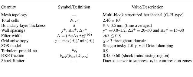
The grid is wall-resolved with y + = 0.8–1.2, Δx + ≈ 20–50 and Δz + ≈ 15–30, ensuring adequate near-wall resolution without requiring wall modelling. To prevent overproduction of eddy viscosity in compression zones, a Ducros-type sensor is used to limit SGS viscosity, which is defined as
 \begin{align} D=\frac{\left(\boldsymbol{\nabla }\boldsymbol{\cdot }u\right)^{2}}{\left(\boldsymbol{\nabla }\boldsymbol{\cdot }u\right)^{2}+\left| \omega \right| ^{2}+10^{-20}}, \end{align}
where
 $D$
≈ 1 identifies purely compressive (shock) regions and
 ${D}$
≈ 0 indicates vortical shear. The limiter ensures that νt
is suppressed near shocks but remains active in shear layers.
The three-dimensional, transient and compressible flow governing equations are solved based on density solvers. In the general coordinate system, the dimensionless detailed governing equation can be expressed as
 \begin{align} \frac{\partial }{\partial t}\!\left(\frac{Q}{J}\right)+\frac{\partial }{\partial \xi }\!\left(F-\frac{M_{\infty }}{\textit{Re}}F_{\upsilon }\right)+\frac{\partial }{\partial \eta }\!\left(G-\frac{M_{\infty }}{\textit{Re}}G_{\upsilon }\right)+\frac{\partial }{\partial \zeta }\!\left(H-\frac{M_{\infty }}{\textit{Re}}H_{\upsilon }\right)=0, \end{align}
where
 $Q=[\overline{\rho },\overline{\rho }\tilde{u},\overline{\rho }\tilde{w},\tilde{E}]^{T}$
is a conservative primitive variable, and
 $J=\partial (\xi ,\eta ,\zeta )/ {}\partial (x,y,z)$
is expressed as the Jacobian determinant of the transformation between the conservative and rectangular coordinate systems. The
 $\overline{\rho } , \tilde{u_{i}} , \tilde{p}$
and
 $\tilde{E}$
variables correspond to the density, velocity component, pressure and total energy in the cartesian coordinate system, respectively. Here, F, G and H are convection flux and the formulae are
 \begin{align} F=\frac{1}{J}\!\left[\begin{array}{c} \overline{\rho }\tilde{U}\\[5pt] \overline{\rho }\tilde{U}\tilde{u}+\xi _{x}\overline{p}\\[5pt] \overline{\rho }\tilde{U}\tilde{v}+\xi _{y}\overline{p}\\[5pt] \overline{\rho }\tilde{U}\tilde{w}+\xi _{y}\overline{p}\\[5pt] \left(\tilde{E}+\overline{p}\right)\tilde{U} \end{array}\right]\!,\quad G=\frac{1}{J}\!\left[\begin{array}{c} \overline{\rho }\tilde{V}\\[5pt] \overline{\rho }\tilde{V}\tilde{u}+\eta _{x}\overline{p}\\[5pt] \overline{\rho }\tilde{V}\tilde{v}+\eta _{y}\overline{p}\\[5pt] \overline{\rho }\tilde{V}\tilde{w}+\eta _{y}\overline{p}\\[5pt] \left(\tilde{E}+\overline{p}\right)\tilde{V} \end{array}\right]\!,\quad H=\frac{1}{J}\!\left[\begin{array}{c} \overline{\rho }\tilde{W}\\[5pt] \overline{\rho }\tilde{W}\tilde{u}+\zeta _{x}\overline{p}\\[5pt] \overline{\rho }\tilde{W}\tilde{v}+\zeta _{y}\overline{p}\\[5pt] \overline{\rho }\tilde{W}\tilde{w}+\zeta _{y}\overline{p}\\[5pt] \left(\tilde{E}+\overline{p}\right)\tilde{W} \end{array}\right]\!, \end{align}
where the expansion formula of
 $\tilde{U} , \tilde{V} , \tilde{W}$
and
 $\tilde{E}$
in (2.6) is (2.7)–(2.10). Top label ‘
 $\overline{\,}$
’ indicates direct filtering procedure and ‘∼’ indicates Favre filtering procedure.
 \begin{align} \tilde{U}=\xi _{x}\tilde{u}+\xi _{y}\tilde{v}+\xi _{z}\tilde{w}, \\[-26pt] \nonumber \end{align}
 \begin{align} \tilde{V}=\xi _{x}\tilde{u}+\xi _{y}\tilde{v}+\xi _{z}\tilde{w} , \\[-26pt] \nonumber \end{align}
 \begin{align} \tilde{W}=\xi _{x}\tilde{u}+\xi _{y}\tilde{v}+\xi _{z}\tilde{w}, \\[-26pt] \nonumber \end{align}
 \begin{align} \tilde{E}=\frac{\overline{\rho }\tilde{T}}{\gamma \left(\gamma -1\right)}+\frac{1}{2}\overline{\rho }\tilde{u_{k}}\tilde{u_{k}} , \end{align}
where F ν , G ν and H ν are viscous flux, which are defined as
 \begin{align} F_{\upsilon }=\frac{1}{J}\!\left[\begin{array}{c} 0\\[5pt] \xi _{\textit{xi}}\tilde{\sigma }_{i1}\\[5pt] \xi _{\textit{xi}}\tilde{\sigma }_{i2}\\[5pt] \xi _{\textit{xi}}\tilde{\sigma }_{i3}\\[5pt] \xi _{\textit{xi}}B_{i} \end{array}\right]\!,\quad G_{\upsilon }=\frac{1}{J}\! \left[\begin{array}{c} 0\\[5pt] \eta _{\textit{xi}}\tilde{\sigma }_{i1}\\[5pt] \eta _{\textit{xi}}\tilde{\sigma }_{i2}\\[5pt] \eta _{\textit{xi}}\tilde{\sigma }_{i3}\\[5pt] \eta _{\textit{xi}}B_{i} \end{array}\right]\!,\quad H_{\upsilon }=\frac{1}{J}\! \left[\begin{array}{c} 0\\[5pt] \zeta _{\textit{xi}}\tilde{\sigma }_{i1}\\[5pt] \zeta _{\textit{xi}}\tilde{\sigma }_{i2}\\[5pt] \zeta _{\textit{xi}}\tilde{\sigma }_{i3}\\[5pt] \zeta _{\textit{xi}}B_{i} \end{array}\right]\!. \end{align}
The ideal gas equation and the Sutherland formula (Vanna, Picano & Benini Reference Vanna, Picano and Benini2020) for calculating the molecular viscosity coefficient
 $\tilde{\mu }(T)$
are used for the closed equation, as expressed as
 \begin{align} \overline{p}&=\frac{\overline{\rho }\tilde{T}}{\gamma }, \end{align}
 \begin{align} \tilde{\mu }(T)&=\tilde{T}^{\frac{3}{2}}\left(\frac{T_{0}+S}{T+S}\right)\!, \end{align}
where T
0 is the thermodynamic temperature equal to 273.15 K and S = 110.4 K is the empirical parameter. Here,
 $\tilde{\sigma _{\textit{ij}}}$
and the viscous stress tensor
 $\tilde{\tau _{\textit{ij}}}$
expressed respectively as
 \begin{align} \tilde{\sigma _{\textit{ij}}}&=\tilde{\tau _{\textit{ij}}}-\tau _{\textit{ij}}^{\textit{SGS}}, \end{align}
 \begin{align} \tilde{\tau _{\textit{ij}}}&=2\tilde{\mu }\tilde{S_{\textit{ij}}}-\frac{2}{3}\tilde{\mu }\tilde{S_{kk}}\delta _{\textit{ij}}, \end{align}
where
 $\tilde{\mu }$
is the dynamic viscosity coefficient of the fluid.
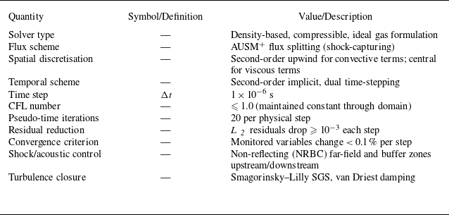
The steady calculation is based on the 3-Dcompressible Reynolds-averaged Navier–Stokes (RANS) equation, and the two-equation eddy viscosity model (k-ω SST) is used for fluid turbulence. The steady convergence result is taken as the initial transient calculation. The ideal gas is set as a fluid medium. The kinetic viscosity calculation equation selects the Sutherland viscosity. The advection upstream splitting method (AUSM) was chosen as the 3-D flux splitting scheme. The momentum equation and energy equation of the spatial control volumes are discretised by a second-order upwind scheme. A second-order implicit scheme is adopted to dispose of the transient equation. The CFL of the transient calculation is fixed at 1 and the number of iterations of the time step is 20. Dual time-stepping ensures per-iteration residual reduction ≥ 10−3 and monitor stability < 0.1 %. Refinement to different time step size changed STLE r.m.s. by < 3 % and phase by < 2°, confirming time-step convergence and statistical consistency. The numerical-scheme and solver parameters used in the LES computations are shown in table 2.
Numerical-scheme and solver parameters used in the LES computations.

2.3. Mesh independence study and solver validation
To eliminate the influence of grid resolution on flow characteristics and to balance computational accuracy with time efficiency, a grid independence study was conducted. A multi-block structured hexahedral mesh with O-type topology around the isolator walls and H-blocks in the main duct was used. Near-wall layers are prismatic with smooth expansion towards the core. Three different grid resolutions were selected for this analysis: grid 1 (1.23 × 10⁶ cells), grid 2 (2.46 × 10⁶ cells) and grid 3 (4.88 × 10⁶ cells). Sparse and dense grids differ by a factor of 4. The experimental conditions are consistent with the simulation conditions, in which the inlet pressure P 0 is set to 4.8 bar, the outlet pressure P b is set to 3 bar and the stagnation temperature T 0 is fixed to 293 K. The curve of the bottom wall centreline pressure in figure 3 shows the distribution of the three grids. The vertical coordinate is wall pressure normalised with P 0. The pressure deviation of the grids in the isolator is large, and the fit of the medium grid and the dense grid is better, which proves that the medium grid can satisfy the calculation accuracy. Considering the calculated time cost, grid 2 was chosen as the grid for subsequent simulation work.
Comparison of static pressure distributions along the centreline of the bottom wall for three grids.

Time step size independence study.

Three kinds of time steps are selected for the time step size independence study for LES as exhibited in figure 4: Δt = 1 × 10⁻⁵ s, Δt = 1 × 10⁻⁶ s and Δt = 5 × 10⁻⁷ s. Within 1 ms, Δt = 1 × 10⁻⁵ s differs greatly from the other time steps. Here, Δt = 1 × 10⁻⁶ s is sufficient for transient calculation, so this study fixed Δt = 1 × 10⁻⁶ s as the time step. All unsteady variables were stored at every step, giving an effective sampling frequency of 1 MHz (Nyquist = 500 kHz). Each record spans 10 ms, corresponding to a spectral resolution of 100 Hz. This temporal resolution is sufficient to capture all shock-train and acoustic oscillations.
Based on grid 2, in transient simulation, the SGS heat flux uses Pr t = 0.9. Wall-based spacings are y + = 0.8–1.2, Δx + = 20–50 and Δz + = 15–30. The local filter width Δ = (ΔxΔyΔz)(1/3) yields Δ/δ ≲ 0.8 based on the measured boundary-layer thickness δ ≈ 3.5, while the grid-anisotropy ratio χ< 3 throughout the isolator. RKEF confirms that the resolved fraction dominates in the shock-train and shear-layer regions, demonstrating adequate spatial resolution for the present flow physics. The specific LES grid-resolution and quality metrics are presented in table 3.
LES grid-resolution and quality metrics.

The experimental and simulation results are verified to prove the reliability of the calculation method, as demonstrated in figure 5. The results are well fitted, proving that the k-ω SST turbulence model can better predict the specific location and energy level of the shock train.
Comparison of static pressure distributions along the centreline of the bottom wall between computational and experimental results.

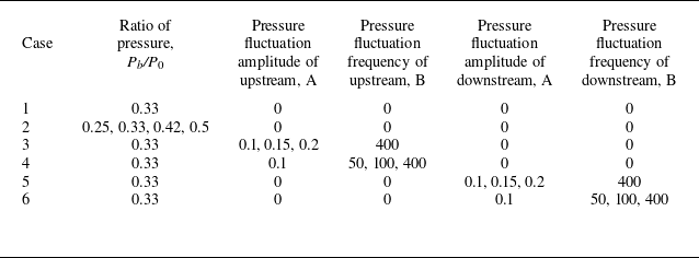
Summary of all conditions.

2.4. Condition statement and flow conditions
The purpose of the current study is to explore the effect of unsteady oscillation on a shock train in the isolator. Self-excited oscillation and forced oscillation cases are studied separately, as shown in table 4. In this paper, P 0 is maintained at 4.8 bar and T 0 = 293 K for all conditions. The research on self-excited oscillation is divided into two parts. In Case 1, the self-excited oscillation with a pressure ratio of 0.33 is analysed in depth. In Case 2, the pressure ratio of upstream and downstream is changed to explore the effect of pressure ratios on shock train self-excited oscillation. The forced oscillation behaviour of the shock train is investigated by introducing a pressure disturbance at the upstream and downstream far fields of the isolator. The amplitude and frequency of the upstream pressure disturbance and the downstream pressure disturbance were studied in Cases 3 to 6. The first is to analyse the upstream and downstream interference modes to the shock train, and the second is to quantitatively and qualitatively analyse the influence of pressure amplitude and frequency on the shock train behaviour. The law of upstream pressure fluctuation selects a sinusoidal function, which is expressed as
 \begin{align}P=P_0(1+A\,\sin(2\pi Bt)).\end{align}
The law of downstream pressure fluctuation selects a sinusoidal function, which is expressed as
 \begin{align}P=P_b(1+A\,\sin(2\pi Bt)).\end{align}
The amplitude of the excitation is denoted by A and ranges from 0.1 to 0.2. The frequency of the fluctuation is denoted by B and ranges from 50 to 400 Hz. For upstream pressure fluctuations, P 0 is fixed at 4.8 bar. For downstream pressure fluctuations, P b is fixed at 1.6 bar.
3. Results and discussion
3.1. Self-excited oscillation of shock train
A total flow time of 10 ms is calculated by the LES method for Case 1, with all boundary conditions remaining unchanged. The shock train oscillates back and forth in the isolator over time. Figure 6 shows the Mach number contours at various
 $x/L$
slices over time. Between 5.5 and 6.9 ms, the unsteady behaviour of the shock train is observed, with significant periodic oscillations. Due to the interaction between the incoming flow and vortices, the unsteady flow in the mixing region lacks a distinct pattern. The Mach number contours slice at
 $x/L$
= 0.63 confirm the oscillation’s periodicity and the three-dimensional characteristics of the STLE are captured. At T = 5.5 ms and 6.9 ms, the Z-direction distribution shows supersonic regions in the central region, while the region near the upper and bottom walls remains subsonic. The STLE overall exhibits an hourglass-like ‘x’ shape. Boundary layer separation at the shock train’s corner intensifies, with this trend increasing along the flow direction and accompanied by angular vortex region expansion. The complex unsteady flow in the mixing region disrupts the separation vortex region developed in the shock train region, leading to intensified self-excited oscillations.
Mach contours at various
 $x/L$
slices over time.

Figure 7 presents Mach number contours of shock train oscillations and vortex distributions within the isolator. Figure 7(a) displays Mach number contours of the shock train oscillations, illustrating their behaviour along the flow direction. At T = 5.5–5.7 ms and 6.7–6.9 ms, the shock train moves upstream. Under an adverse pressure gradient, the shock train’s post-compression shape remains well defined. During T = 5.7–6.7 ms, the shock train propagates downstream under a favourable pressure gradient. Figure 7(b) depicts Mach number contours superimposed with vortex distributions during shock train oscillations. Vortex formation positions are identified using the Q criterion (Hunt, Wray & Moin Reference Hunt, Wray and Moin1988; Silva & Pereira Reference Silva and Pereira2008). The Q criterion approximates vortex positions in the 3-D isolator and the associated Mach number distributions. Small vortices forming in the subsonic region behind each shock wave are clearly resolved. At the corner domain of the isolator, the vortex is close to the wall surface. Near the corners of the isolator, vortices adhere to the wall surface, exhibiting slow motion and small sizes. The Mach number here is lower than that of the vortices at the centre. Vortex sizes near the isolator centre increase with higher Mach numbers. The pronounced asymmetry in vortex motion along the flow direction underscores the importance of analysing 3-D unsteady features.
Mach contours of shock train oscillations and vortex distributions within the isolator: (a) Mach contours for the shock train oscillations; (b) Mach contours with vortex distribution for the shock train oscillations.

Static pressure oscillations at multiple monitoring locations.

To further investigate the self-excited oscillation characteristics of the shock train, figure 8 presents pressure distribution oscillations under static pressure monitoring at multiple locations. Pressure data from four upper-wall monitoring points are analysed: U 3 (front leading shock), U 5 (near leading shock), U 9 (behind leading shock) and U 15 (in the mixing region). The U 3 upstream region remains supersonic, exhibiting minimal and stable pressure fluctuations. As airflow enters the shock train region, the pressure profile undergoes abrupt changes and pressure oscillations are intense yet periodic near U 5. Supersonic flow induces small-range pressure jitter, whereas shock waves trigger sharp pressure fluctuations. As the flow develops downstream in the shock train, it is affected by three key factors: oscillations at the shock train leading edge, oscillation signals from the interaction of multiple internal shocks and flow oscillations in the subsonic/supersonic mixing region. Thus, the pressure at U 9 shows small-range jitter alongside wide-range fluctuations. At U 15 in the mixing region, subsonic–supersonic flow superposition creates highly complex and unsteady dynamics. Consequently, pressure oscillates violently near P/P 0 = 0.25 without discernible periodicity.
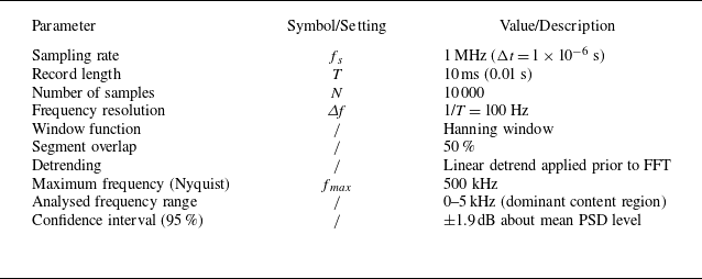
Parameters used for FFT-based PSD analysis.

PSD distributions along the centreline of the upper and bottom walls.

PSDs of wall pressure were computed using ANSYS Fluent’s built-in FFT-based routine. Each signal contained 10 000 samples over a 10 ms record (sampling rate = 1 MHz), yielding a frequency resolution of 100 Hz. A Hanning window with 50 % overlap and linear detrending was applied to minimise leakage and bias. The resulting spectra possess 95 % confidence intervals of approximately ±1.9 dB, confirming the statistical reliability of the identified dominant frequencies in the 0–5 kHz range. Parameters used for FFT-based PSD analysis in ANSYS Fluent are shown in table 5. The total sampling covers several full cycles of the dominant 0.8–1.2 kHz oscillation, ensuring convergence of the primary low-frequency modes relevant to the present analysis. Figure 9 presents PSDs along the centreline of the upper and bottom walls. The pressure self-excited oscillation of the isolator is within the range of 0–5000 Hz, which is in the low-frequency oscillation range. Upper and bottom wall pressure distributions exhibit marked differences. Below 2000 Hz, intense shock train oscillations dominate, yielding higher pressure energy in the shock train region versus the mixing region. In the 2000–5000 Hz range, complex vortex dynamics (formation/rupture) and boundary layer separation enhance pressure energy in the mixing region relative to the shock train region. As seen in figure 9(b), the bottom wall has marginally greater pressure oscillation energy than the upper wall in both regions, accompanied by a high-frequency distribution bias. Higher pressure energy levels and high-frequency components suggest the shock train develops lateral deviation when the isolator operates unsteadily.
Figure 10 presents the shear stress distribution on both upper and bottom walls in attached and separated flow regions at a pressure ratio of 0.33 (Case 1). The wall shear stress component in the X-direction (aligned with incoming flow) is analysed. Positive shear stress values (shown in red) indicate attached flow regions and negative values (shown in blue) represent separated flow regions. The periodic nature of shock train self-excited oscillations is evident from time-varying boundary layer separation positions. Asymmetric shear stress distributions between the upper and bottom walls reveal shock train asymmetry. Shock train oscillations differ fundamentally from flow oscillations in the mixing region. The shock train exhibits large-amplitude oscillations, whereas the mixing region flow alternates between subsonic and supersonic states with frequent boundary layer separation/reattachment, producing small-amplitude oscillations. Notable flow differences exist at symmetric centreline positions (Z = ±2.5 mm and Z = ±5 mm). This demonstrates the inherently 3-D feature of shock train oscillations. Three-dimensional modelling is required to accurately capture these flow phenomena. Flow propagates radially from the centreline to the isolator corners, with expanding corner vortices in the separation region.
Contours of attached and separated flow regions: (a) isolator upper wall; (b) isolator bottom wall.

3.2. Effect of upstream and downstream pressure ratios
The flow conditions upstream and downstream of the isolator are primarily determined by thermodynamic parameters, including temperature and pressure. Variations in these parameters lead to corresponding changes in shock train morphology within the isolator. This investigation examines four pressure ratio conditions (P b /P 0 = 0.25, 0.33, 0.42, 0.5) using the LES method to simulate isolator operation in a scramjet engine. The characteristic self-excited oscillation modes of the shock train were compared across pressure ratios through detailed data analysis. Figure 11 presents Mach number contours at T = 4.2 ms, illustrating shock train oscillations at each pressure ratio. Decreasing pressure ratios result in increased shock wave spacing and more pronounced oblique shock structures. For P b /P 0 = 0.25, the shock train system exhibits incomplete development within the isolator. Shock wave interactions under this condition cause combustion instability in the downstream combustor. Consequently, this case proves unsuitable for the practical operation of the scramjet.
Mach contours of the shock train oscillations for different pressure ratios.

Figure 12 presents the unsteady pressure variation of different pressure ratios of upstream and downstream (Case 2). At a pressure ratio of 0.25, monitoring point U 5 is located upstream of the shock train and the self-excited oscillation amplitude is attenuated in the supersonic region. As the pressure ratio increases, the shock train moves upstream; in this case, U 5 lies near the STLE, and the shock train’s self-excited oscillation mode differs distinctly from those in the supersonic region and mixing region. Large amplitude and regular fluctuations demonstrate the highly periodic motion of the STLE. With further increase in the pressure ratio, monitoring points within the mixing region exhibit self-excited oscillations comprising small-scale fluctuations superimposed on large-scale variations. Furthermore, small-scale pressure oscillations intensify progressively at monitoring points nearer to the downstream region.
Unsteady pressure variation of different pressure ratios of upstream and downstream.

Pressure PSD distributions for four pressure ratio conditions.

Figure 13 displays the pressure PSDs for four pressure ratio conditions (Case 2). Fourier transformation of pressure data from monitoring point U 5 reveals that PSD trends directly correlate with pressure variations. Figure 13(a) presents the pressure PSD in the upstream supersonic region, demonstrating the suppression of oscillation development in this flow regime. Figure 13(b) illustrates the pressure PSD distribution near the STLE, where self-excited oscillations reach maximum intensity. Conversely, figures 13(c) and 13(d) reveal suppressed self-excited oscillations within the mid-section of the shock system. While individual shock waves convect with the large-scale shock train motion, their relative positions deviate from the shock train’s absolute movement pattern. The observed suppression of self-excited oscillations in the shock train suggests that inter-shock interactions attenuate oscillation amplitudes. In the mixing region, supersonic flow separation and subsequent vortex interactions generate highly complex unsteady flow patterns. The value of pressure PSD magnitudes in the mixing region exceeds those within the shock train system. All observed pressure PSD fluctuations occur below 5000 Hz, characteristic of low-frequency phenomena.
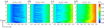
Figure 14 presents contours indicating the variation of static pressure on the upper wall, effectively demonstrating the self-excited oscillation phenomena of the shock train under four pressure ratios. The results demonstrate that increasing pressure ratios produce more regular shock train oscillations, with reduced oscillation periods and progressive shock train shortening. The self-excited oscillation mode of the wake in the mixing region is different from that of the shock train region. While sharing identical oscillation periods, the complex flow dynamics in the mixing region amplify small-scale oscillation components.
Contours indicating the variation of static pressure on the upper wall.

Figure 15 displays contours showing the regions of attached and separated flow under four pressure ratio conditions, quantitatively characterising the shock train length and oscillatory displacement range. Comparative analysis between P b /P 0 = 0.25 and 0.5 conditions reveals that for the shock train at higher pressure ratio, the self-excited oscillations exhibit enhanced regularity while their frequency rises, accompanied by a progressive reduction in shock train length. Higher P b /P 0 produces longer-lived, broader separated patches (flatter streaks), consistent with a thicker, more dissipative buffer that attenuates downstream-to-upstream transmission and diminishes STLE response.
Contours showing the regions of attached and separated flow for four pressure ratio conditions.

Probability distribution histogram of STLE position and the probability distribution curve fitted by the Gaussian formula.

Figure 16 shows the probability distribution histogram of STLE position and the probability distribution curve fitted by the Gaussian formula. The STLE position was determined from the streamwise gradient of the centreline wall pressure using Savitzky–Golay differentiation with mild low-pass filtering; an independent iso-surface of ∣∇ρ∣ provided consistent locations within one grid spacing. The histogram statistically quantifies STLE position occurrence frequency, while the Gaussian fitting characterises the spatial distribution characteristics of shock train leading edge positions. Under adverse pressure gradient conditions, the shock train demonstrates gradual upstream movement. Conversely, when subjected to favourable pressure gradients, the shock train exhibits rapid downstream propagation accompanied by flow structure diffusion. After maintaining a downstream position, the shock train subsequently initiates gradual upstream migration. The motion resistance under adverse pressure gradients significantly exceeds that under favourable gradients, resulting in non-normal distribution characteristics. Furthermore, increasing pressure ratios produce more concentrated STLE position distributions.
Pressure standard deviation distributions along the upper wall for different pressure ratio conditions.

The pressure standard deviation
 $\sigma _{P/{P_{0}}}$
can reflect the stability of the information, and the formula is
 \begin{align} \sigma _{P/{P_{0}}}=\sqrt{\frac{1}{N}\sum _{i=1}^{N}\big(x_{P/{P_{0}},i}-\mu _{\kern-1.5pt P/{P_{0}}}\big)^{2}}, \end{align}
where N represents the time step and equals 10 000. Here,
 $x_{P/{P_{0}},i}$
represents the value of the non-dimensionalised pressure at a certain time and
 $\mu _{P/{P_{0}}}$
represents the average value of the static pressure in the total time after the undimensionalisation.
Figure 17 is the pressure standard deviation distributions along the upper wall for different pressure ratio conditions. The oscillation intensity and position of the shock train are determined based on the standard deviation distribution characteristics. The isolator flow field comprises four distinct regions: the supersonic region, the shock train region, the mixing region and the subsonic region. Upstream of the STLE in the supersonic region, oscillation behaviour is suppressed, with suppression effects intensifying near the STLE location. A sharp increase in pressure standard deviation near STLE indicates intensified self-excited oscillations. Downstream of multiple shock waves, the standard deviation gradually decreases as shock train oscillations weaken. In the mixing region, boundary layer separation, vortex motion and upstream shock wave interactions together intensify flow oscillations and increase the amplitude of pressure standard deviation. Conversely, the subsonic region demonstrates progressively decreasing standard deviation values due to diminished upstream disturbance effects. Comparative analysis shows that smaller pressure ratios correspond to longer shock trains and identifiable average positions. As evidenced in figure 17(a), reduced pressure ratios extend the shock system length, enabling better resolution of pressure fluctuations. The second shock wave position can be identified through characteristic standard deviation variations. This standard deviation analysis method provides an innovative approach for shock train research.
3.3. Effect of upstream pressure amplitude
Pressure perturbations are introduced at the isolator inlet to investigate upstream effects on shock train forced oscillations. The perturbations follow a sinusoidal waveform with controlled variations in both amplitude and frequency. Three distinct perturbation amplitudes (A = 0.1, 0.15 and 0.2; Case 3) and frequencies (B = 50 Hz, 100 Hz and 400 Hz; Case 4) are implemented at the upstream boundary, as illustrated in figure 18. The computational simulation spans a total duration of 10 ms under a constant downstream-to-upstream pressure ratio of 0.33.
Upstream pressure disturbance control function: (a) pressure variations for different upstream amplitudes at 400 Hz; (b) pressure variations for different upstream frequencies at fixed 0.1 amplitudes.

Figure 19 displays the Mach number contours capturing shock train oscillations under upstream pressure conditions of A = 0.1 with B = 400 Hz, where the temporal evolution of the STLE position exhibits periodic oscillatory behaviour between T = 5.5 ms and T = 6.7 ms. In the initial phase (5.5–5.8 ms), the shock train moves upstream against the flow; it then accelerates rapidly downstream (5.8–6.4 ms) to reach maximum forced oscillation displacement. The oscillation cycle completes as the shock train returns to its initial position during the final phase from 6.4 to 6.7 ms, demonstrating a complete periodic oscillation under these controlled conditions.
Mach contours capturing shock train oscillations for the upstream pressure condition of A = 0.1 with B = 400 Hz.

Pressure variation curves at the U 5 over time for different upstream pressure disturbance amplitudes.

Figure 20 presents pressure variation curves at the U 5 monitoring point over time under different upstream pressure disturbance amplitudes at a fixed frequency of 400 Hz (Case 3), examining three amplitude conditions (0.1, 0.15 and 0.2). The pressure oscillation amplitude at U 5 exhibits a direct correlation with increasing upstream disturbance amplitude. Comparative analysis shows that pressure distribution curves under disturbed conditions have smaller oscillation magnitudes than the self-excited oscillations of the undisturbed shock train, confirming upstream pressure perturbations significantly influence shock train dynamics. Specifically, under the A = 0.1 and B = 400 Hz condition, the upstream disturbance modifies the shock train natural oscillation state, yielding pressure values lower than those observed in unperturbed self-excited oscillations.
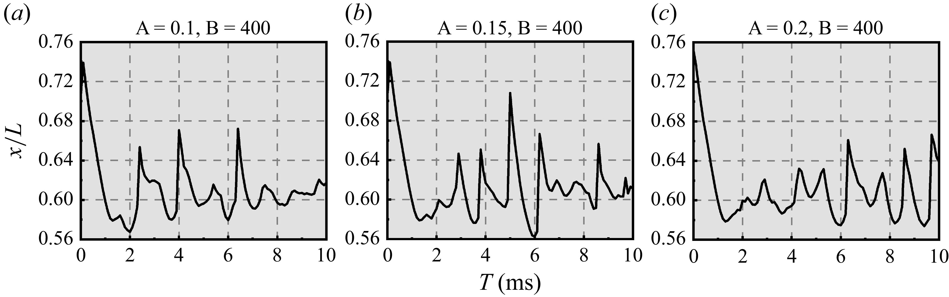
Figure 21 shows the variation curves of the STLE position with time under different upstream pressure disturbance amplitudes. As the disturbance amplitude increases, the STLE position changes exhibit distinct patterns at corresponding time instances, showing no consistent similarity across amplitudes. The shock train oscillations demonstrate clear asynchronicity in both spatial position and temporal evolution, revealing that upstream amplitude variations produce non-uniform effects on oscillation characteristics. This complex forced oscillation behaviour stems from the combined influence of inherent isolator flow unsteadiness and external pressure perturbations, resulting in multifaceted shock train dynamics.
Variation curves of STLE position with time for different upstream pressure disturbance amplitudes.

Figure 22 displays the pressure PSD curves at monitoring point U 5 for different upstream pressure disturbance amplitudes. The shock train oscillations represent a superposition of self-excited oscillation and forced oscillation induced by upstream pressure perturbations. Comparative analysis reveals that the oscillatory pressure energy under all three disturbance amplitudes remains lower than that of undisturbed self-excited oscillations, demonstrating the suppressive effect of upstream perturbations on shock train oscillations. However, within this suppressed state, increasing the disturbance amplitude leads to intensified shock train oscillations. Notably, the peak oscillation frequency remains largely unaffected by variations in upstream pressure amplitude. The pressure PSD distribution spans 0–2000 Hz, confirming low-frequency oscillation characteristics consistent with the undisturbed shock train self-excited oscillation behaviour.
Pressure PSD curves at U 5 for different upstream pressure disturbance amplitudes.

Figure 23 presents the contours indicating the variation of static pressure on the upper wall under different upstream pressure disturbance amplitudes. In the region of
 $x/L$
= 0.5–0.6, the upstream pressure pulsation is transmitted downstream and the number of pressure transmission events is affected by the upstream interference period. Within a duration of 10 ms and at a frequency of 400 Hz, four complete cycles of pressure fluctuations occurred and four distinct pressure transmission phenomena were observed in all three conditions. When the pressure disturbance reaches its minimum value, the pressure wave propagates to the downstream shock train. As the upstream pressure amplitude increases, the magnitude of reduction in the minimum pressure value becomes larger, resulting in stronger transmission of upstream interference effects downstream.
Contours indicating the variation of static pressure on the upper wall for different upstream pressure disturbance amplitudes.

Figure 24 presents the contours showing the regions of attached and separated flow under different upstream disturbance amplitudes. The shear stress distribution along the upper wall centreline serves to identify flow separation and reattachment locations. The shock train oscillation exhibits distinct characteristics from the flow oscillation in the mixing region, enabling clear differentiation between the shock train region (
 $x/L$
= 0.6–0.8) and the mixing region (
 $x/L$
= 0.8–1.0) based on shear stress distribution. As the upstream disturbance amplitude increases, both the shock train region and the mixing region experience a slight reduction in flow separation area.
Contours showing the regions of attached and separated flow for different upstream disturbance amplitudes.

The standard deviation serves as an effective indicator of data dispersion and is particularly valuable for quantifying shock train oscillation intensity. Figure 25 presents the pressure standard deviation distributions along the upper wall varying upstream pressure disturbance amplitudes. The analysis reveals that pressure standard deviations in the supersonic region, shock train region and mixing region all increase with growing upstream disturbance amplitude, while concurrently exhibiting a reduction in shock train length. In the supersonic region, the pressure standard deviation progressively decreases until reaching a minimum value just upstream of the shock train leading edge. As the flow enters the shock train region, characterised by a sharp pressure rise, all three test conditions demonstrate suppressed oscillations near x = 0.23 m. This behaviour suggests the presence of an extensive, stable boundary layer separation zone near this pressure monitoring location that remains unaffected by variations in upstream disturbance amplitude. Within the mixing region, the pressure standard deviation follows the characteristic wall pressure distribution profile. The sustained pressure rise in this region amplifies the flow oscillation amplitude, consistent with the observed enhancement of pressure fluctuations under increased disturbance conditions.
Pressure standard deviation distributions along the upper wall vary with upstream pressure disturbance amplitudes.

3.4. Effect of upstream pressure frequency
Three conditions (Case 4) were investigated with an upstream pressure disturbance amplitude of A = 0.1 at frequencies of B = 50 Hz, 100 Hz and 400 Hz. Figure 26 presents the pressure variation curves at the U 5 monitoring point over time under different upstream pressure disturbance frequencies, derived from processed static pressure data. The analysis reveals that higher upstream disturbance frequencies correspond to reduced peak and trough values in the wall pressure fluctuations over time. For the 50 Hz condition, the pressure variation completes half a sine function cycle within the total flow duration. The peak and trough values of pressure oscillations exhibit a characteristic trend of initial increase followed by decrease along the frequency variation curve, which mirrors sinusoidal behaviour. For slow changes in boundary conditions, such as those in low-frequency disturbances, the shock train adapts promptly and maintains synchronisation with the upstream disturbance pattern. At 100 Hz, the temporal variation of minimum pressure follows a sinusoidal trend. However, at the higher frequency of 400 Hz (four complete cycles), the shock train motion becomes unable to respond sufficiently quickly. This response delay prevents the shock train’s inherent unsteady motion from adapting to the rapidly changing upstream boundary conditions. The shock train’s inherent resistance to external disturbances during movement introduces both oppositional forces and temporal lag in its oscillations, ultimately leading to oscillation suppression. Comparative analysis shows that relative to undisturbed conditions, increasing upstream disturbance frequencies produce progressively more disordered shock train oscillations while simultaneously enhancing oscillation suppression effects. This frequency-dependent behaviour demonstrates a clear trade-off between disturbance response fidelity and oscillation control effectiveness.
Figure 27 presents the variation curves of STLE position with time under different upstream pressure disturbance frequencies. During the initial 2–4 ms period, corresponding to the first complete oscillation cycle of the shock train, the shock train movement exhibits distinct periodic characteristics. Comparative analysis reveals that upstream frequency disturbances only minimally affect the periodic oscillation of the shock train leading edge when compared with undisturbed conditions. At B = 50 Hz, the upstream excitation exerts a relatively minor influence, with the shock train’s oscillatory behaviour maintaining periodicity similar to that observed in undisturbed conditions. The oscillation patterns demonstrate remarkable consistency with the baseline case, suggesting that low-frequency disturbances preserve the shock train’s inherent dynamic characteristics.
Pressure variation curves at the U 5 over time for different upstream pressure disturbance frequencies.

Variation curves of STLE position with time for different upstream pressure disturbance frequencies.

Figure 28 presents the pressure PSD curves at monitoring point U 5 for different upstream pressure disturbance frequencies. In contrast to the effects of amplitude variations on shock train oscillations, increasing frequency demonstrates a suppression effect on oscillation energy. Comparative analysis reveals that upstream frequency disturbances stabilise shock train motion relative to its natural self-excited oscillations, with higher frequencies exhibiting stronger suppression characteristics. These observations indicate that upstream frequency disturbances exert a beneficial influence on shock train oscillation control within the isolator. Notably, frequency variations show a negligible impact on the peak frequency of shock train pressure PSD. The pulsation signal remains concentrated within the 0–2000 Hz range, aligning with the shock train’s natural self-excited oscillation frequency and maintaining a low-frequency oscillatory state.
Pressure PSD curves at U 5 for different upstream pressure disturbance frequencies.

Figure 29 displays the contours indicating the variation of static pressure on the upper wall under different upstream pressure disturbance frequencies. The analysis reveals that the frequency of pressure pulsation transmission from upstream to downstream increases proportionally with disturbance frequency. Consistent with the behaviour observed under upstream amplitude variations, pressure signal transmission occurs at minimum pressure values, with distinct first and fourth transmission signals identifiable at B = 100 Hz and B = 400 Hz conditions, respectively. Within the shock train region (
 $x/L$
= 0.6–0.8), the pressure distribution gradient difference decreases with higher upstream disturbance frequencies, indicating a corresponding reduction in shock train oscillation intensity. This observed attenuation of pressure gradient variations directly correlates with weakened shock train oscillations under increased frequency conditions.
Contours indicating the variation of static pressure on the upper wall for different upstream pressure disturbance frequencies.

Figure 30 presents the contours showing the regions of attached and separated flow under different upstream disturbance frequencies. The analysis demonstrates that increasing upstream excitation frequency promotes stabilisation of the boundary layer within the isolator. This stabilisation effect is characterised by the formation of large-scale vortical structures that effectively dampen shock train oscillations. These observations indicate that elevated upstream frequency disturbances exert a significant suppressive effect on shock train oscillatory behaviour.
Contours showing the regions of attached and separated flow for different upstream disturbance frequencies.

Pressure standard deviation distributions along the upper wall vary with upstream pressure disturbance frequencies.

Figure 31 displays the pressure standard deviation distributions along the upper wall varying upstream pressure disturbance frequencies. At the 50 Hz condition, the shock train responds promptly to upstream disturbances, where the combined effect of self-excited and forced oscillations leads to more intense oscillations compared with the undisturbed case. For higher frequency conditions (100 Hz and 400 Hz), when the upstream pressure reaches low values, the shock train tends to move upstream. However, the presence of adverse pressure gradients significantly hinders this upstream movement, creating a mismatch between the upstream disturbance characteristics and the internal flow dynamics of the isolator. This phase discrepancy exerts a detrimental effect on shock train oscillation. Additionally, the spatial analysis reveals that while the shock train occupies the region between x = 0.19 and 0.26 m under undisturbed conditions, it shifts downstream to x = 0.2–0.27 m when subjected to upstream frequency disturbances. This systematic downstream displacement demonstrates that upstream frequency perturbations induce an overall shift in shock train position.
Probability distribution histogram of STLE position and the probability distribution curve fitted by the Gaussian formula for different upstream disturbance conditions.

The statistical analysis encompassed five distinct conditions, including three upstream amplitude variations (B = 400 Hz with A = 0.1, 0.15, 0.2; Case 3) and three upstream frequency variations (A = 0.1 with B = 50, 100, 400 Hz; Case 4). Figure 32 presents the probability distribution histogram of STLE position and the probability distribution curve fitted by the Gaussian formula under different upstream disturbance conditions. Comparative analysis with undisturbed conditions reveals that all five disturbed cases exhibit more symmetrical STLE position distributions, demonstrating that upstream unsteady disturbances facilitate shock train upstream propagation by reducing flow resistance. Frequency-dependent analysis shows that higher upstream disturbance frequencies (B = 50, 100, 400 Hz at constant A = 0.1) produce progressively more concentrated STLE position distributions. This frequency-dependent focusing effect confirms that increased upstream disturbance frequencies effectively suppress shock train oscillations and promote flow stabilisation. Conversely, amplitude-dependent analysis demonstrates that greater upstream disturbance amplitudes (A = 0.1, 0.15, 0.2 at constant B = 400 Hz) result in increasingly dispersed STLE position distributions. This amplitude-dependent dispersion effect indicates that stronger upstream disturbances amplify shock train leading edge oscillations, consistent with the observed destabilisation trend under high-amplitude conditions.
3.5. Effect of downstream pressure amplitude
A comprehensive investigation was performed to analyse shock train oscillations induced by downstream pressure disturbances within the isolator. The study examined these oscillations over a total computational duration of 10 ms. For Case 5, the analysis focused on downstream amplitude disturbances across four complete pressure cycles, backpressure P b is 1.6 bar, as illustrated in figure 33(a). Case 6, presented in figure 33(b), explored the effects of disturbances with amplitude A = 0.1 over varying numbers of cycles (0.5, 1 and 4 cycles).
Downstream pressure disturbance control function: (a) pressure variations for different downstream amplitudes at 400 Hz; (b) pressure variations for different downstream frequencies at fixed 0.1 amplitudes.

Figure 34 displays the Mach contours capturing shock train oscillations under the downstream pressure condition of A = 0.1 with B = 400 Hz. Detailed examination of the temporal evolution between 6.4 and 7.8 ms reveals asymmetric displacement behaviour, with significantly greater downstream movement occurring during at 6.8–7.6 ms compared with the upstream displacement observed in both the preceding (6.4–6.8 ms) and subsequent (7.6–7.8 ms) intervals. The shock train demonstrates a complete oscillation cycle comprising three distinct phases: initial upstream propagation (6.4–6.8 ms), followed by rapid downstream movement with subsequent flow stabilisation and finally gradual upstream recovery to its original position. This dynamic process highlights the fundamental asymmetry in shock train motion, where downstream propagation occurs more rapidly and with greater morphological variability than the more constrained upstream movement, indicating substantially different flow resistance characteristics in each direction. Throughout the entire oscillation cycle, the shock system maintains remarkable structural integrity, showing no significant changes in the shock sequence configuration despite the substantial positional variations.
Mach contours capturing shock train oscillations under the downstream pressure condition of A = 0.1 with B = 400 Hz.

Figure 35 presents the pressure variation curves at the U 5 monitoring point over time under different downstream pressure disturbance amplitudes. During the initial phase (T = 1–3 ms), all cases exhibit consistent pressure oscillation characteristics. Similar to upstream amplitude effects, increasing downstream disturbance amplitude amplifies pressure fluctuations near STLE at point U 5. However, downstream disturbances induce more periodic forced oscillations in the shock train compared with upstream excitations. The high-amplitude condition (A = 0.2, B = 400 Hz) demonstrates particularly noteworthy behaviour: while producing more regular oscillations than low-frequency downstream disturbances, it simultaneously generates significantly larger oscillation amplitudes. The analysis suggests that optimal flow control should prioritise both minimising oscillation energy and reducing spatial displacement of shock train motion.
Pressure variation curves at the U 5 over time for different downstream pressure disturbance amplitudes.

Variation curves of STLE position with time for different downstream pressure disturbance amplitudes.

Figure 36 illustrates the variation curves of STLE position with time under different downstream pressure disturbance amplitudes. The analysis reveals that the condition with A = 0.1 and B = 400 Hz demonstrates superior oscillation suppression effectiveness compared with other tested conditions, exhibiting significantly reduced STLE position fluctuations. This suppression performance surpasses all previously examined upstream disturbance cases. A comparative evaluation with equivalent upstream disturbance conditions (A = 0.1, B = 400 Hz) shows that while both scenarios produce similar pressure variation patterns, the downstream disturbance exhibits two distinct advantages: first, the absolute pressure variation magnitude remains smaller as it is superimposed on the baseline backpressure; second, it achieves better oscillation suppression than corresponding upstream disturbances. These findings demonstrate the stronger influence of downstream disturbances on shock train dynamics. Furthermore, the study identifies an amplitude-dependent response characteristic: larger downstream pressure pulsation amplitudes generate more pronounced STLE oscillations while simultaneously producing more regular motion patterns. This regularity progressively approaches the characteristic behaviour of shock train self-excited oscillations, suggesting that increased disturbance amplitudes may effectively ‘entrain’ the shock train into more predictable oscillation modes. The results highlight the complex interplay between disturbance amplitude, oscillation regularity and the system’s inherent self-excited oscillation characteristics.
Figure 37 presents the pressure PSD curves at monitoring point U 5 for different downstream pressure disturbance amplitudes, obtained through Fourier transform analysis of unsteady wall pressure data. At A = 0.1 and B = 400 Hz, the PSD of the shock train pressure is lower than that under other conditions, indicating effective oscillation suppression that outperforms upstream disturbance effects. With increasing downstream pressure amplitude, the shock train oscillation energy shows corresponding enhancement. Comparative analysis of identical parameter sets (A = 0.15, B = 400 Hz and A = 0.2, B = 400 Hz) reveals that downstream conditions exert greater influence on shock train oscillations on the isolator than their upstream counterparts. The results demonstrate a positive correlation between downstream amplitude magnitude and shock train oscillation intensity, with more pronounced effects relative to upstream disturbances. Under downstream amplitude effects, all pressure PSD values remain below those of the shock train’s self-excited oscillation condition, with frequency components concentrated below 2000 Hz.
Pressure PSD curves at U 5 for different downstream pressure disturbance amplitudes.

Contours indicating the variation of static pressure on the upper wall for different downstream pressure disturbance amplitudes.

Figure 38 presents the contours indicating the variation of static pressure on the upper wall under different downstream pressure disturbance amplitudes. The downstream disturbance mechanism exhibits fundamentally different characteristics from upstream interference. Unlike upstream disturbances that directly impact the shock train region along the flow direction, downstream perturbations propagate upstream through a stepwise transmission process from the mixing region to the shock train region in the reverse flow direction. The downstream unsteady influence primarily affects the mixing region, where the complex flow dynamics amplify the disturbance before its transmission to the upstream shock train region. This amplification process results in distinct flow responses, where increased downstream amplitude variations produce more regular and intensified shock train motions. The observed regularity and intensity of shock train movement demonstrate a direct correlation with the magnitude of downstream pressure fluctuations.
Contours showing the regions of attached and separated flow for different downstream disturbance amplitudes.

Figure 39 displays the contours showing the regions of attached and separated flow under different downstream disturbance amplitudes. The flow attachment and separation zones are determined by positive and negative X-directional wall shear stress values, respectively. Analysis reveals that the STLE undergoes oscillatory motion about
 $x/L$
= 0.6. The study demonstrates that increased downstream excitation amplitudes produce two significant effects: first, they enlarge the attached flow area in the mixing region (
 $x/L$
= 0.8–1); second, this enhanced flow attachment strengthens flow signal transmission, consequently intensifying shock train oscillations. These observations establish a clear relationship between downstream disturbance magnitude and shock train dynamic response, where greater excitation amplitudes systematically modify both flow attachment characteristics and oscillation intensity.
Figure 40 presents the standard deviation distribution of wall pressure along the upper surface for different downstream disturbance amplitudes. The analysis reveals several key findings regarding shock train behaviour. Near the STLE position, increasing downstream frequency produces a negative feedback effect on shock train oscillation. The data demonstrate a direct correlation between downstream disturbance amplitude and oscillation intensity, with larger amplitudes generating more pronounced shock train movements. The small-amplitude condition (A = 0.1) exhibits the most rapid pressure rise in the mixing region. Comparative analysis with upstream amplitude variations shows distinct response characteristics: while upstream amplitudes show positive correlation with pressure standard deviation in the supersonic region, downstream disturbances do not propagate upstream to significantly affect the STLE. Consequently, all three downstream conditions maintain consistent pressure standard deviation distributions in the supersonic region. Furthermore, flow oscillation amplitudes throughout the isolator are systematically smaller under downstream amplitude effects compared with equivalent upstream amplitude conditions. This consistent reduction in oscillation magnitude confirms that downstream disturbances provide superior suppression of shock train oscillations relative to upstream perturbations. The improved suppression effectiveness manifests across all monitored regions of the flow field.
Pressure standard deviation distributions along the upper wall vary with downstream pressure disturbance amplitudes.

3.6. Effect of downstream pressure frequency
Figure 41 presents the pressure variation curves at the U 5 monitoring point over time under different downstream pressure disturbance frequencies. Comparative analysis of the three frequency conditions (50 Hz, 100 Hz and 400 Hz; Case 6) reveals that higher downstream frequencies correspond to reduced peak pressures. The influence mechanisms of downstream and upstream frequency disturbances share both similarities and distinct characteristics. The common feature is that elevated disturbance frequencies in both cases effectively suppress shock train oscillation amplitudes while intensifying small-scale oscillatory behaviour, thereby reducing overall oscillation regularity. However, a key difference emerges in the STLE pressure response: unlike the upstream 50 Hz condition, where minimum pressure fluctuations vary significantly, downstream frequency variations maintain relatively stable minimum pressure levels at P/P 0 = 0.5, regardless of frequency changes. This behaviour results from the complex signal transformation occurring during upstream propagation. When downstream disturbances travel countercurrent towards the shock train, the mixing region’s internal flow dynamics modify the original signal. Consequently, the pressure pulsation reaching the upstream shock train region is no longer a simple, frequency-preserved signal as observed in downstream-travelling disturbances. The combined effects of multiple shock wave interactions and boundary layer separation create a highly coupled pressure signal at the STLE location. While the shock train oscillation pattern does not directly mirror the downstream frequency variation, the downstream disturbances nonetheless effectively suppress oscillation amplitudes. This demonstrates that the suppression mechanism operates through complex flow interactions rather than simple frequency matching.
Pressure variation curves at the U 5 over time for different downstream pressure disturbance frequencies.

Figure 42 displays the variation curves of STLE position with time under different downstream pressure disturbance frequencies. The results demonstrate that increasing downstream frequency effectively suppresses STLE oscillations, with higher frequencies corresponding to progressively smaller oscillation amplitudes. The downstream frequency disturbances propagate sequentially through the mixing region and shock train region, modifying the isolator’s internal flow field and thereby influencing STLE oscillation characteristics. A comparative analysis with upstream frequency disturbances (Case 4) reveals that downstream frequency variations (Case 6) produce a more pronounced suppression effect on shock train oscillations across all tested conditions (B = 50, 100 and 400 Hz). This enhanced suppression highlights the distinct influence of downstream perturbations on shock train dynamics compared with upstream disturbances.
Variation curves of STLE position with time for different downstream pressure disturbance frequencies.

Figure 43 displays the pressure PSD curves at monitoring point U 5 for different downstream pressure disturbance frequencies. Similar to upstream frequency effects, increasing downstream frequency restricts shock train oscillations. However, a key difference emerges: downstream low-frequency disturbances (B = 50 and 100 Hz) amplify wall pressure PSD values near the STLE, indicating a nonlinear relationship between downstream frequency variation and shock train oscillation intensity. These low-frequency pressure variations intensify shock train oscillations. At high frequency (B = 400 Hz), the shock train’s unsteady motion exhibits a delayed response that cannot keep pace with the rapid downstream pressure variations. This response lag results in an apparent suppression effect in the statistical analysis. The findings demonstrate that downstream frequency influences shock train behaviour through fundamentally different mechanisms than upstream frequency disturbances.
Pressure PSD curves at U 5 for different downstream pressure disturbance frequencies.

Figure 44 presents the contours indicating the variation of static pressure on the upper wall under different downstream pressure disturbance frequencies. The results demonstrate significant differences between flow oscillation behaviour in the mixing region and shock train oscillations, both in periodicity and modal characteristics. As downstream frequency increases, flow oscillations decrease within the
 $x/L$
= 0.8–0.9 range. The frequency variation signal propagates upstream to the shock train region (
 $x/L$
= 0.6–0.8), suppressing shock train oscillations. However, downstream frequency disturbances cannot propagate further upstream to affect the supersonic region, where the pressure distribution remains relatively constant over time. Unlike upstream frequency disturbances that transmit signals downstream when pressure changes reach minimum values, downstream disturbances exhibit different transmission characteristics. While all upstream frequency conditions suppress shock train oscillations, downstream frequency variations produce more complex effects. Combined with transonic flow phenomena in the isolator, low-frequency downstream disturbances intensify shock train oscillations, whereas high frequencies effectively suppress them.
Contours indicating the variation of static pressure on the upper wall for different downstream pressure disturbance frequencies.

Figure 45 displays contours showing the regions of attached and separated flow under different downstream disturbance frequencies. As downstream excitation frequency increases, the separation area progressively expands between the shock train and mixing regions. Pressure signal propagation through this separated flow effectively suppresses STLE oscillation phenomena.
Contours showing the regions of attached and separated flow for different downstream disturbance frequencies.

Figure 46 shows the pressure standard deviation distributions along the upper wall varying downstream pressure disturbance frequencies. Higher downstream frequencies reduce the shock train’s self-excited oscillation amplitude. At 50 Hz, the shock train moves upstream as a whole and its oscillations intensify following a downstream disturbance. Downstream pressure changes disrupt the shock train’s original dynamic equilibrium, leading to a time lag in its dynamic response. When external disturbances match the shock train’s internal state, complex unsteady phenomena occur, making forced oscillation amplitudes exceed undisturbed self-excited oscillation. As frequency increases further, the shock train oscillations conflict with downstream frequency changes, confining oscillations to smaller displacement ranges. Downstream frequency variations produce similar effects to upstream disturbances. High-frequency pressure variations effectively suppress shock train oscillations and enhance isolator flow stability.
Pressure standard deviation distributions along the upper wall vary with downstream pressure disturbance frequencies.

Figure 47 shows the probability distribution histogram of STLE position and the probability distribution curve fitted by the Gaussian formula under different downstream disturbance conditions (Case 5 and Case 6). The STLE position distribution becomes more concentrated with increasing downstream frequency. Under the condition of A = 0.1 and B = 400 Hz, the STLE positions cluster around
 $x/L$
= 0.59, indicating this pressure disturbance helps stabilise shock train motion. Larger downstream amplitudes cause more dispersed STLE position distributions, directly increasing shock train displacement and intensifying oscillations. Five different conditions were compared, including both amplitude and frequency variations. The results demonstrate that the downstream pressure condition of A = 0.1 and B = 400 Hz most effectively suppresses shock train oscillations in the isolator.
Probability distribution histogram of STLE position and the probability distribution curve fitted by the Gaussian formula for different downstream disturbance conditions.

4. Summary and conclusions
The oscillatory behaviour of the shock train in a three-dimensional rectangular diverging isolator, encompassing both self-excited and forced oscillations, is systematically investigated using the LES method. The self-excited oscillation analysis examines multiple upstream-to-downstream pressure ratios, with one representative case selected for detailed study. User-defined codes control the pressure amplitude and frequency at both upstream and downstream far-field boundaries of the isolator. Principal conclusions drawn from this investigation are as follows.
-
(i) The self-excited oscillation phenomenon of the shock train in the isolator was investigated using the LES method at a fixed pressure ratio of P b /P 0 = 0.33. The results demonstrate three-dimensional characteristics in the shock train oscillations within the flow field. Oscillation distribution patterns vary spatially due to differing influences from the upstream supersonic inflow and downstream mixing region. Flow field variations in the isolator were analysed by comparing four pressure ratio conditions (P b /P 0 = 0.25, 0.33, 0.42, 0.5). The results reveal distinct oscillation modes in different flow regions. Flow oscillations in the supersonic region exhibit small, stable amplitudes, while pressure oscillations at the shock train leading edge display clear regularity and periodicity. The shock train oscillations are influenced by three primary factors: the large-scale regular fluctuations originating from the leading edge of the shock train, the modified oscillations resulting from interactions between shock waves within the shock train itself, and the large-scale oscillations generated by complex flows in the mixing region. These combined influences create a composite oscillation pattern that represents the superposition of multiple distinct oscillation modes.
-
(ii) Through controlled variations in the amplitude and frequency of upstream and downstream pressure disturbances, the forced oscillation characteristics of the shock train under environmental influences were investigated. Results show that at an upstream frequency of 400 Hz, increasing the upstream pressure amplitude enhances the oscillation intensity in the supersonic region, shock train region and mixing region, a trend supported by the upper wall pressure standard deviation distribution. When the pressure disturbance amplitude is fixed at 0.1, the upstream disturbance frequency (B = 50, 100, 400 Hz) does not exhibit a singular influence on shock train oscillations. The shock train displays slow oscillation response characteristics. Under low upstream interference frequencies, the shock train adapts to external variations, resulting in oscillation intensification. Conversely, higher upstream pressure frequencies induce movement lag as the shock train fails to accommodate rapid external disturbances, consequently reducing oscillation amplitudes. The upstream pressure variations maintain isolator flow field oscillations within the low-frequency range, consistent with self-excited oscillation characteristics. Notably, the external upstream interference frequency shows no direct correlation with the oscillation frequency, while increased interference amplitude shifts the shock train’s self-excited oscillations towards relatively higher frequency regions.
-
(iii) The shock wave motion intensifies with increasing downstream disturbance amplitude. External influences propagate from the mixing region upstream, inducing regular fluctuations in shock train oscillations whose amplitude grows with downstream amplitude. Shock train oscillations are increasingly suppressed with higher downstream pressure disturbance frequencies. Low-frequency disturbances amplify shock train oscillations, whereas high-frequency disturbances suppress shock train movement. Downstream pressure frequencies suppress shock train oscillations more effectively than upstream frequencies. While upstream and downstream pressure amplitude and frequency changes produce similar effects on shock train oscillations, their underlying mechanisms differ. Pressure pulsation propagation differs between supersonic and subsonic regions. Forward and reverse pressure gradient transmission directions additionally influence shock train oscillation intensity. External high-frequency pressure disturbances maintain relatively stable shock train conditions in the isolator, with downstream high-frequency disturbances proving more effective than upstream ones.
Funding
The authors are grateful for the support from the National Natural Science Foundation of China (Grant No. 52206058), Natural Science Foundation of Zhejiang Province (Grant No. LQ22E060002), Zhejiang Sci-Tech University Foundation (Grant No. 21022247-Y), and Zhejiang Key Laboratory of Multiflow and Fluid Machinery (Grant No. 2024E10006).
Declaration of interests
We have no conflicts of interest to disclose.
Data availability statement
The data that support the findings of this study are available from the corresponding author upon reasonable request.