Crop growth models

There are many crop growth models for crop yield prediction and management (Steduto, Reference Steduto2003; Panday, Reference Panday2014). In these models, the main physiological and physical processes include the development of leaf area, light interception and dry matter production, partitioning of dry matter, effects of soil water dynamics and, in some, nutrients (Kabat et al., Reference Kabat, Marshall, van den Broek, Vas and van Keulen1995).

The potato growth model in MAPP simulates the development and growth process of a single plant, including stages of tuber sprouting, appearance and expansion of leaves, initiation of tubers and senescence. It calculates the fraction of radiation intercepted as a function of leaf area index, and then relates this to the dry matter production, which the soil moisture deficit affects (Jefferies and Heilbronn 1995). In MAPP, the dry matter partitioning is modelled using a thermal-time dependent ‘harvest index’ and the total yield is calculated by estimating the tuber dry matter concentration as a function of soil moisture deficit and temperature.

The growth model calculates a water balance daily from inputs of precipitation and irrigation and losses by evaporation from both soil and crop, and the total extractable soil water is obtained by defining the maximum rooting depth and multiplying it by the extractable soil moisture volume fraction. Nutrient dynamics and the dependence of plant growth on nutrients are not currently modelled in MAPP.

The tuber size distribution (TSD) model in MAPP is an empirical model, a truncated normal distribution. It estimates the proportion by fresh weight of daughter tubers produced in any specified size range, where tuber size is defined either by square mesh riddle size (mm) or by the fresh weight (g) of the individual tuber. In order to predict a TSD, one needs to know both the total yield and total number of daughter tubers produced which are greater than 15 mm square mesh riddle size. This is usually generated from mid-season manual digs.

The growth and yield model and the tuber size distribution model of the MAPP were developed by the James Hutton Institute (formerly Scottish Crop Research Institute), Dundee, Scotland. The growth and yield model is designed to simulate an individual plant that is representative of the field average. It does not aggregate over multiple individuals nor does it model the interaction between neighbouring plants. However, it is known that there is variability within a field in many of the drivers of the model, particularly the canopy development and size and the availability of soil water supply to the crop (Allaire et al., Reference Allaire, Cambouris, Lafond, Lange, Pelletier and Dutilleul2014).

Spatialisation - conceptual spatial crop modelling

There are several potential ways that the MAPP model (or any crop model) could be made spatial. It could be simply spatialised through running the existing model independently at a finer spatial resolution ignoring neighbourhood effects, or converted into a true spatial model that runs at a finer spatial scale and incorporates information on the effect of the neighbourhood in the modelling process. The latter, modifying existing models by integrating spatial interactions, is preferable but more complex and not practical at the current stage.

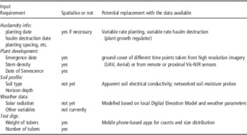
The possibility for running the model at a finer spatial scale lies in the availability of spatial data. Currently MAPP uses aspatial environmental input data, including weather data and soil profile information, for the simulation of each field/farm. However, fine resolution spatial data such as soil electrical conductivity, crop growth imagery, and sampling data of soil moisture is increasingly available. Table 1 compares the current model input with current available data, highlighting the gap between the spatial data available and the data required for modelling at a finer spatial scale. However, there exists a potential to make use of the spatial data for spatial modelling. The challenge now lies in which scale the model should be applied and how to replace the input with the spatial data we have.

Possible scales to run the MAPP model at include but are not limited to:

1. 1. Individual plant

2. 2. Bed planting spacing (~3 m*3 m grid)

3. 3. An arbitrary pixel size (e.g. 5 m² or 10 m²)

4. 4. Management units

5. 5. Whole field

To determine which scale is the best to run the model is a complex task, depending on multiple criteria: including the purpose, data availability and model requirements. Generally, the purpose is to provide growers with as accurate information as possible for their decision-making, so the finest scale is preferred. Since the original model simulates individual plants, applying the model at a scale smaller than a single plant scale is not sensible. The whole field, the original scale of output of the MAPP models, is obviously not appropriate for this project either.

Considering the nature of the basic MAPP model, the more reasonable choices would be choices 1 and 2. However, due to a lack of corresponding input data at those scales, these choices would be better regarded as a long-term target for crop production and management. As a simplified interim step, modelling crop development and yield/tuber distribution can be done at a MU level. This MU scale is variable, depending on the number of management units specified. This is normally limited to a maximum of 3 or 4 units, and often only 2 (Pedroso et al., Reference Pedroso, Taylor, Tisseyre, Charnomordic and Guillaume2010), due to the feasibility of machinery operations.

With advances in agricultural machinery, in the foreseeable future, variable-rate operations are unlikely to be a factor that limits the scale of SSCM. It is more likely that limitations in scale will be imposed by the ability to process, interpret and generate decisions from the multitude of information sources now available to growers/agronomists. In this study, the intent was to identify, without considering the limitation of operation, what management unit level maximally integrates the data available and is the most accurate when applying the models to estimate the yield and graded yields of the field and assist with the field management.

Spatial variability is the driver for model spatialisation. The other challenge (as mentioned above) is to find spatially varying data that reflect different environmental conditions and management activities of different areas within a field as model input to run the model spatially for more accurate prediction and decision-making. In many cases, available spatial data are non-identical to required input variables, so investigating how to transform them becomes the main task. To identify what spatial data to use to replace some certain model inputs and how, their influence on the crop yield needs to be analysed and appropriate methods for their inclusion to replace the original homogeneous variables need to be determined.

With in-season stratified sampling of crops, it is possible to test the spatial variability of their dry matter, tuber weight and number, plant and stem density, etc. Also, with stratified heterogeneity test (Wang et al., Reference Wang, Christakos and Hu2009), we can see if they are significantly different among the strata, derived from soil ECa. If yes, then the ECa probably is the reason for the heterogeneity. This test could also be done based on strata other than those used for sampling, even on the strata generated with different criteria, e.g. planting date. In this way, an optimum MU level would be found for a criterion (here each unit does not have to be contiguous) and potential influential factors would be identified.

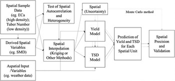
As mentioned above, quantification of influential factors as model input is desirable and challenging, requiring a thorough exploration through lab experiments or data analysis. Once this is achieved, the crop models can be applied to the determined units with varied input. Decisions that can be made using the model for the field as a whole can be made for each unit, for example, when to irrigate, where and how much. Figure 1 illustrates the whole process, in which model spatialisation is realised through several steps: determination of optimal units, preparation of varied input, model application to spatial units and at the end, uncertainty analysis.

Figure 1

Spatialisation through applying the models to each spatial unit

Some experimental results

A survey was performed in a field in Yorkshire, UK for a preliminary case study and the results are listed in Tables 2 and 3, where sampling data of yield, dry matter, stems and canopy cover have been processed and analysed. In this field, multiple data collections have been conducted at 100 sampling points that were selected based on an existing apparent soil electrical conductivity map (EC_a).

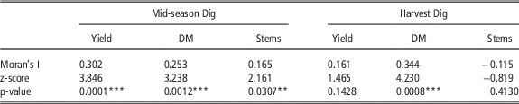
Spatial autocorrelation helps understand the degree to which one object is similar to other nearby objects. Moran’s I (Index) (Moran, Reference Moran1950) is used to measure spatial autocorrelation. As we can see from Table 2, the yield, DM and stems of the first dig have significant spatial autocorrelation, while only the DM variable exhibits autocorrelation at harvest. Through cluster and outlier analysis in ArcGIS (ESRI, Redlands CA, USA), which identifies statistically significant hot/cold spots and outliers using the Anselin Local Moran’s I statistic, it is easy to find that the high value clusters are all concentrated on the northern section of the field.

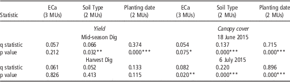
The field was then divided into two units, a northern and a southern unit, and tested for stratified heterogeneity with the q statistic (Wang et al., Reference Wang, Zhang and Fu2016). The results are presented in Table 3, where the greatest q value is 0.896, which means that 89.6% of variance of the canopy cover measured on July 6, 2015 can be explained by the division and is statistically significant. Farmer’s planting at the northern part approximately 3 weeks earlier than the southern was identified as a major reason for this variance.

Therefore, the influence factor leading to the difference between these two units is planting date. Since planting date is directly a model input, the process of transforming the influence factor as an input can be omitted and the varied input for planting date are directly formed by the two actual dates. Applying the growth model and graded model to the two units with the varied planting dates, yield and tuber size distribution predictions were generated from the model, and the accuracy can be calculated through comparing with the observed unit averages.

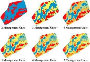
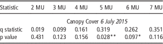
Although the above is a simple case study, in principle, it embodies the essence of the spatialisation process in Figure 1. The situation could be more complex if the influence factors are environmental, not managerial. For example, with soil EC_a, the field can be split into management units (classes) using k-means classification (Taylor et al., Reference Taylor, Whelan and McBratney2007) (Fig. 2) in a number of ways. Testing their stratified heterogeneity using the canopy cover of 6 July, 2015, it can be seen that the most statistically significant q value is 0.31, indicating that 5 management units is optimal (see Table 3). Statistically this level is more reasonable than others for transforming soil ECa as varied input for model simulation. Combining varied input (layers), managerial or environmental, could lead to a finer spatial scale for model application.

Figure 2

Potential Management Units based on classification for 2–7 classes using the SoilEC_a data