Introduction
Understanding and quantifying the rates of production and the postmortem fates of skeletal carbonates is important to many aspects of geology, paleobiology, and ecology. The interaction between carbonate production, loss, reworking, and burial determine the overall carbonate budget of ecosystems dominated by carbonate producers (Pandolfi et al. Reference Pandolfi, Connolly, Marshall and Cohen2011; Perry et al. Reference Perry, Murphy, Kench, Edinger, Smithers, Steneck and Mumby2014; Waldbusser and Salisbury Reference Waldbusser and Salisbury2014), the availability of skeletal debris in benthic habitats and the preservation of reef framework (Powell et al. Reference Powell, Kraeuter and Ashton-Alcox2006; Waldbusser et al. Reference Waldbusser, Powell and Mann2013), the temporal resolution and completeness of death assemblages and accuracy of paleoecological indices (Bush and Bambach Reference Bush and Bambach2004; Hunt Reference Hunt2004; Olszewski Reference Olszewski2004; Kidwell et al. Reference Kidwell, Best and Kaufmann2005; Tomašových and Kidwell Reference Tomašových and Kidwell2010; Olszewski 2012; Berkeley et al. Reference Berkeley, Perry, Smithers and Hoon2014; Tomašových et al. Reference Tomašových, Kidwell, Foygel Barber and Kaufman2014), the reconstruction of baseline states and onset of anthropogenic habitat changes (Kowalewski et al. Reference Kowalewski, Avila Serrano, Flessa and Goodfriend2000; Kidwell Reference Kidwell2007), and carbonate accumulation rates and flux in depositional systems (Scarponi et al. Reference Scarponi, Kaufman, Amorosi and Kowalewski2013; Kemp and Sadler Reference Kemp and Sadler2014; Kosnik et al. Reference Kosnik, Hua, Kaufman and Zawadzki2014; Olszewski and Kaufman Reference Olszewski and Kaufman2015). Similar dynamics apply to the postmortem fates of any organic remains, such as diatoms, bones, pollen, and wood (Cameron Reference Cameron1995; Kavvadias et al. Reference Kavvadias, Alifragis, Tsiontsis, Brofas and Stamatelos2001; Leorri and Martin Reference Leorri and Martin2009; Terry Reference Terry2010; Terry et al. Reference Terry, Li and Hadly2011; Dawson et al. Reference Dawson, Smithers and Hua2014).
Postmortem skeletal loss rates are evaluated in two ways: (1) by tracking the disintegration of individual shells through time in laboratory and field experiments, usually over short periods of a few days to years (Cummins et al. Reference Cummins, Powell, Stanton and Staff1986; Glover and Kidwell Reference Glover and Kidwell1993; Dittert and Henrich Reference Dittert and Henrich2000; Powell et al. Reference Powell, Kraeuter and Ashton-Alcox2006, Reference Powell, Callender, Staff, Parsons-Hubbard, Brett, Walker, Raymond and Ashton-Alcox2008; Waldbusser et al. Reference Waldbusser, Steenson and Green2011; Ford and Kench Reference Ford and Kench2012); and (2) by measuring frequency distributions of the radiocarbon-calibrated ages of shells in mixed-layer death assemblages sampled at a single time (Meldahl et al. Reference Meldahl, Flessa and Cutler1997; Olszewski Reference Olszewski1999; Kidwell et al. Reference Kidwell, Best and Kaufmann2005; Kosnik et al. Reference Kosnik, Hua, Kaufman and Wüst2009, Reference Kosnik, Kaufman and Hua2013; Tomašových et al. Reference Tomašových, Kidwell, Foygel Barber and Kaufman2014). Short-term experiments are extremely valuable, and can calibrate preservation indices that track down-core changes in preservation (Conan et al. Reference Conan, Ivanova and Brummer2002). However, the postmortem age-frequency distributions (AFDs) produced by the latter approach reveal the full temporal dimension of time-averaged accumulation: molluscan, brachiopod, and foraminiferal shells sampled from modern seabeds, for example, can be hundreds of years to a few thousands or tens of thousands of years old (for reviews, see Kosnik et al. Reference Kosnik, Hua, Kaufman and Wüst2009; Kidwell and Tomasovych Reference Kidwell and Tomasovych2013). AFDs thus provide decadal- to millennial-scale perspectives on the net effects of dissolution, bioerosion, diagenetic precipitation and burial in the mixed layer. The models used to quantify rates of skeletal loss using AFDs are represented either by a simple exponential model where the rate of loss is constant in time (Meldahl et al. Reference Meldahl, Flessa and Cutler1997; Kosnik et al. Reference Kosnik, Hua, Kaufman and Wüst2009) or by models with temporally declining loss rates (Olszewski Reference Olszewski2004; Tomašových et al. Reference Tomašových, Kidwell, Foygel Barber and Kaufman2014).
However, the shapes of AFDs are almost certainly determined not simply by rates of disintegration and burial but also by temporal changes in biological production (Flessa et al. Reference Flessa, Cutler and Meldahl1993; Krause et al. Reference Krause, Barbour, Kowalewski, Kaufman, Romanek, Simoes and Wehmiller2010; Dexter et al. Reference Dexter, Kaufman, Krause, Barbour Wood, Simoes, Huntley, Yanes, Romanek and Kowalewski2014). Both simple exponential and time-varying models of shell loss assume a constant rate of input of individuals into a death assemblage over the duration of time-averaged accumulation, and so their estimates of loss rates might be inaccurate. Populations can wax and wane on many time-frames, such as in response to annual and decadal climate cycles, millennial-scale climate-driven changes in range size and location, and anthropogenic stresses such as acidification, nutrification, and the introduction of non-native species. All of these fluctuations can occur within the window of time averaging. Such changes can be captured by AFDs, thus providing a unique tool for one of the major goals in conservation paleobiology and historical ecology, namely inferring changes in abundance and productivity over the recent past. However, disintegration and burial likely modulate the signature of temporal history in production. It is thus important to assess how loss and production jointly affect the shapes of AFDs if we are to accurately infer past production pulses as well as disintegration and burial rates from death assemblages encountered in the surficial mixed layer of the sedimentary record.
Here, first, we expand three models of shell loss within and below the mixed layer, introduced in Tomašových et al. (Reference Tomašových, Kidwell, Foygel Barber and Kaufman2014), that assume constant production, using these to assess the consequences of variable production on estimates of loss rates. These models can estimate loss rates using either: (1) information on the distributions of ages of dead individuals at the time of their disintegration, such as derived from time-lapse experiments; or (2) information on the distributions of ages of dead individuals sampled in a mixed layer at a single time (AFDs). Second, we assess how the dynamics of production and loss can be jointly inferred from mixed-layer death assemblages sampled from modern seabeds and landscapes. We present two models that couple temporal variation in production with shell loss: (1) a single past pulse of production, following a normal distribution trajectory, subjected both to constant loss and to a more realistic model where per-capita loss rates decline over time; and (2) a scenario of production that started at a specific time (e.g., initial flooding of a marine habitat) and terminated at another time (e.g., anthropogenic stress), subjected both to constant loss and to temporally declining loss.
With these approaches, we assess: (1) the extent to which estimates of loss rates based on constant-production models are robust to variation in production, and (2) the extent to which temporal variability in production could be masked by loss rates, thus providing useful heuristics for conservation paleobiology to detect true changes in skeletal production. We focus on a single species, the aragonitic deposit-feeding bivalve Nuculana taphria that prefers a relatively narrow, 19–56 m depth zone on the southern California shelf. If this species migrated with post-glacial sea-level rise, tracking its preferred shallow waters, then its AFDs should vary significantly in shape across the modern shelf if changes in the timing of production control the shape of mixed-layer AFDs.
Material and Methods
Death Assemblages
A total of 253 dead specimens of Nuculana taphria were acquired from Van Veen grab samples taken at 15 sites on the continental shelf between Santa Barbara and San Diego during the Southern California Bight Regional Monitoring Program in 2003 (Ranasinghe et al. 2007) and during a sediment mapping project of the San Diego shelf conducted by the City of San Diego in 2004 (Stebbins et al. Reference Stebbins, Schiff and Ritter2004) (Fig. 1). Each grab had a surface area about 0.1 m2 and penetrated approximately 10 cm into the seabed. We randomly selected 25 specimens per grab from samples that contained more than 25 specimens of N. taphria. We pooled samples to four assemblages that correspond to four water depth intervals along the bathymetric gradient, including: (1) seven sites at 23–31 m (n=105 shells), (2) three sites at 40–48 m (n=66), (3) five sites at 51–58 m (n=61), and (4) two sites at 89 m (n=46). A subset of the samples from the 23 to 58 m depth range was analyzed by Tomašových et al. (Reference Tomašových, Kidwell, Foygel Barber and Kaufman2014). Here, we add 46 specimens from the two deeper sites (89 m), and exclude two shallow-water sites from the Palos Verdes shelf where habitat modification was severe in the second half of the 20th century (Supplementary Table 1). Knowledge of the preferred water depth of N. taphria is based on our compilation of benthic data from 490 stations on the southern California shelf sampled by Van Veen grabs during publicly funded surveys in 2003 and 2004 (Ranasinghe et al. Reference Ranasinghe, Montagne, Smith, Mikel, Weisberg, Cadien, Velarde and Dalkey2003, Stebbins et al. Reference Stebbins, Schiff and Ritter2004). The proportional abundance of living N. taphria peaks between 19 and 56 m.
Southern California Bight study area and sample sites grouped by water depth interval (coordinates in Supplementary Appendix Table 1). Bathymetric contours in meters.

Radiometric Ages and Calibration of AAR Ratios
All 253 shells of Nuculana taphria were analyzed for the extent of amino acid racemization (AAR) at Northern Arizona University using the procedures of Kaufman and Manley (Reference Kaufman and Manley1998). Eleven specimens were selected for AMS 14C dating at the NOSAMS facility in Woods Hole, using the screening criteria of Kosnik and Kaufman (Reference Kosnik and Kaufman2008). Radiocarbon ages have been converted to calendar years using Calib6.0 (Stuiver and Reimer Reference Stuiver and Reimer1993) and calibrated with the Marine04 data (Hughen et al. Reference Hughen, Baillie, Bard, Bayliss, Beck, Bertrand, Blackwell, Buck, Burr, Cutler, Damon, Edwards, Fairbanks, Friedrich, Guilderson, Kromer, McCormac, Manning, Bronk Ramsey, Reimer, Reimer, Remmele, Southon, Stuiver, Talamo, Taylor, van der Plicht and Weyhenmeyer2004), using a regional marine reservoir correction (∆R) of 234 years (SD=96). The calibration curves were constrained to pass through the origin and the D/L value of live-collected specimens was used as value that determines zero age. The ages are computed as b*([D/L]e−[D/L]alivee), where b is a slope and e is a power-law exponent that minimize: (1) absolute differences between the measured 14C age and the age predicted by the linear relationship between D/Le and the calibrated 14C age, divided by the measured 14C age, and (2) absolute differences between age estimates derived from aspartic and glutamic acid, divided by the measured 14C age. The mean calibrated AAR age (averaged over two calibrations for aspartic and glutamic D/L values, respectively) is weighted by the inverse of the standard error of the age squared. All ages are calibrated relative to AD 2003, when the samples were collected from the seafloor (Supplementary Table 2). Details on specimen preparation, AAR age calibration and the source codes written in R (R Development Core Team 2014) are presented in the Supplement and in Tomašových et al. (Reference Tomašových, Kidwell, Foygel Barber and Kaufman2014).
Model Evaluation
We estimate maximum- likelihood parameters of three models assuming constant production and two truncated-normal models permitting variation in production. Akaike Information Criterion (AIC) values quantify the level of fit and penalize for the number of parameters (Burnham and Anderson Reference Burnham and Anderson2002). However, the mixtures of truncated-normal and exponential densities in the varying-production models represent different classes of models. Therefore, we evaluate the goodness of fit of both of the two varying-production models and the three constant-production models using a G-test. The G-statistic measures the deviation between the observed frequencies and the frequencies expected under a random sampling from the distributions fitted by the five models. Although this test depends on the choice of age binning, varying bin size between 100 and 1000 years leads to similar results, and so we report the values only for bins with 250 years. We also compare the observed estimates of median age and interquartile range with the estimates predicted by models.
Models
We consider three scenarios of loss of skeletal carbonates from the mixed layer (by disintegration and burial) (Fig. 2), each represented by a probability density function of shell ages under an assumption of constant production. Shells can be lost from the mixed layer of the seabed, where taphonomic processes tend to be most intense (i.e., in the taphonomically active zone, TAZ of Davies et al. Reference Davies, Powell and Stanton1989), by two pathways, which are not mutually exclusive: (1) disintegration (caused by any process that damages shells, reducing their taxonomic identifiability); and/or (2) net burial to a deeper sediment zone, eventually to a zone of final burial (caused by any biological or physical process that moves shells downward, away from the TAZ). Loss can also be caused by a third pathway, namely transport to other sites (e.g., Flessa Reference Flessa1998), but this effect is minimized with an increasing spatial extent of sampling: out-of-habitat transport becomes less likely over increasingly large areas. In addition, between-habitat transport of significant numbers of shells is generally limited to a few high-energy or non-level settings (see reviews by Kidwell and Bosence Reference Kidwell and Bosence1991; Kidwell Reference Kidwell2013).
A–C, Three changes in loss rate as a function of shell age in the mixed layer, with A, one-phase model (λ is constant), B, Weibull model (λ declines gradually with time), and C, two-phase model (λ declines abruptly from high λ 1 to a much lower rate λ 2). Loss of shells from the mixed layer can arise from disintegration and/or from burial to deeper layers. The depth of burial within the mixed layer may or may not correlate with shell age. D–F, Three possible scenarios of the two-phase model plotted against sediment depth. D, Shells subject to high λ 1 in the TAZ (white layer) shift by burial to the SZ (gray layer) where they experience much lower λ 2. Variable τ corresponds to net burial rate if shells that are exhumed back to the TAZ but do not retain their λ 2. Sampling gear penetrates into the SZ. E, The same scenario as in (D), but shells exhumed back to the TAZ retain λ 2, e.g., if burial in the SZ is coupled with diagenetic stabilization. Sampling gear not penetrating into the SZ will still encounter shells that reflect the two-phase model. F, the SZ represents a patchy microenvironment favoring diagenetic stabilization. Diagenetic stabilization still results in a decline of λ with time but with little or no burial below the sediment-water interface. Final burial zone (FBZ) denotes a position below the sediment-water interface where shells are beyond the reach of further physical and biogenic reworking, and where further disintegration is determined by the realm of late diagenesis.
If disintegration rates vary vertically or horizontally within the mixed layer, then this layer can be subdivided conceptually into a TAZ with high disintegration rates and a sequestration zone (SZ) with low disintegration rates (e.g., Olszewski Reference Olszewski2004). Our three models differ in the way they account for shell loss via disintegration and/or burial within and below the mixed layer (left three graphs in Fig. 2; adapted from Tomašových et al. Reference Tomašových, Kidwell, Foygel Barber and Kaufman2014). The first model is defined by a single parameter that represents an instantaneous per individual loss rate that is constant in time within the mixed layer (one-phase exponential model), whereas the other two models permit a gradual (Weibull model) or an abrupt (two-phase exponential model) temporal decline in the instantaneous per-individual loss rate. Although sedimentological and biological evidence implies that the loss-rate parameter is dominated by disintegration rather than by burial below the mixed layer in marine systems (Tomašových et al. Reference Tomašových, Kidwell, Foygel Barber and Kaufman2014), the relative contributions of disintegration and burial processes to the loss parameter likely vary as a function of taxa and environments (Terry and Novak Reference Terry and Novak2015).
All three models assume that production is constant. To evaluate the joint effects of variation in production and shell loss, we combine our one-phase and two-phase models of loss described above with (1) a gradual change in production following a normal distribution trajectory; and (2) a stepwise change in production following a rectangular distribution trajectory, with production increasing sharply at one point and then declining sharply at a later point.
Censored age data
When using age data (e.g., AFDs) to estimate the time until the occurrence of some event (here, the timing of loss of a shell from a death assemblage), those age data are considered to be censored if the event of interest did not occur at the actual time when the age data were collected—that is, the event of interest either pre-dates or post-dates the time of sampling (Kleinbaum and Klein Reference Kleinbaum and Klein2005). Right censoring refers to the scenario where the event—here, the loss of individuals from the death assemblage—has not yet occurred: the time to shell loss—i.e., the postmortem shell lifespan—exceeds the observed age at the time of sampling. We focus here on right censoring because the age of shells sampled on the seafloor pre-dates their loss. Left censoring refers to a scenario where the loss of individuals occurred before the age data were sampled (i.e., the time to shell loss is smaller than the observed age). Such censoring would apply where rates of fragmentation are estimated on the basis of the postmortem ages of shell fragments (fragmentation could have occurred at any time prior to sampling), or in time-lapse experiments where rates of loss are inferred from the first sampling when shells are no longer present rather than from the last sampling when they are present.
Figure 3 visualizes the importance of right censoring of postmortem lifespans of shells under conditions of temporally constant production (the postmortem lifespans of shells are represented by horizontal black lines, each bounded by the time of input to and loss from the death assemblage) and a single time of sampling (vertical dashed line). The time of sampling splits postmortem lifespans into right-censored parts (light grey shading) and unsampled parts (dark grey shading). Several features are evident. First, shell age at the time of sampling underestimates the full postmortem lifespans of the shells that are sampled in the mixed layer. This effect decreases the median age of sampled shells relative to the median age of a random selection of shells at the time of their actual loss. Second, shells with shorter lifespans are less likely to be sampled than are shells with longer lifespans. This effect increases the median age of sampled shells relative to the median age of a random selection of shells at the time of their actual loss. These two biases cancel each other in models with constant loss (Fig. 3A): the snapshot AFD produced by sampling shells in the mixed layer at any given moment (gray histogram) provides an accurate estimate of the AFD that would be produced by a random sampling of the true, full lifespans of shells (black histogram in Fig. 3A), with differences in AFD shape arising purely from the effects of finite sampling. In contrast, if loss rates change over time, the snapshot AFD provides a biased estimate of the AFD based on a random sampling of full lifespans (Fig. 3B–C; we use a simple Weibull function to explore the effects). Older shells are more likely to be sampled than younger shells in models with decreasing loss rates (as in the Weibull and two-phase models in Fig. 2; Fig. 3B), and older shells are less likely to be sampled than younger shells in models with increasing loss rates (Fig. 3C). Under conditions of constant production, the right-censored distributions will always monotonically decrease from young to old postmortem ages. The most frequent shells will thus tend to have a ‘zero’ age, that is will fall in the first age bin, regardless of the shape of the underlying non-censored probability density function. That function can be non-monotonic, for example if loss rate increases with time (Fig. 3C).
Visualizing the effects of right censoring on the shape of AFDs sampled at a single time (vertical dashed lines) under constant shell production (with 100,000 shells produced) and A, temporally constant loss rates, B, temporally declining loss rates, and C, temporally increasing loss rates. Black horizontal lines represent individual shells bounded by the time of their input (death) on the left and by the time of their loss on the right. The lengths of lines thus correspond to full postmortem lifespans of shells (for clarity, each plot shows only 2,500 shells). The time of sampling splits the lifespans into: (1) thick light grey bands representing the censored ages of shells (i.e., their right-censored lifespans), and (2) thick dark gray bands representing the unsampled portions of lifespans. Gray histograms represent snapshot AFDs, i.e., the expected frequency distributions of (right-censored) shells ages at the time of their sampling on the seafloor, and the black histograms represent the expected frequency distributions of a random sample of the full, true lifespans of shells. In contrast to a scenario with constant loss (A), the snapshot AFD provides a biased estimate of the AFD based on a random sampling of full lifespans if loss rates change over time (B, C).
Therefore, AFDs sampled at a single time are different from the AFD based on a random sampling of the full postmortem lifespans of shells (i.e., the kind of data more likely to be generated by time-lapse experiments); only in the special case when the loss rate is constant would a snapshot AFD match the AFD of true lifespans (Fig. 3A). Probability density functions used to estimate times to loss on the basis of censored age data thus differ from those using non-censored age data. Analyses of survivorship in population biology (Colchero and Clark Reference Colchero and Clark2012) and evolutionary paleobiology (Gilinsky Reference Gilinsky1988; Foote and Raup Reference Foote and Raup1996; Ezard et al. Reference Ezard, Pearson, Aze and Purvis2012) also correct for age censoring. This issue thus has consequences for many paleobiological studies that work with age data.
Models with Constant Production
For all three constant-production models, we present both: (1) non-censored and (2) right censored density functions because both types of age data can be collected in taphonomic and paleobiologic analyses. Non-censored functions can be used to quantify loss rate by measuring shell ages at the time of their loss. This kind of data—or a very close approximation of it, depending upon the spacing of successive samplings—is produced by experiments that track individual shells or cohorts of shells through time (e.g., Cummins et al. Reference Cummins, Powell, Stanton and Staff1986; Kotler et al. Reference Kotler, Martin and Liddell1992; Glover and Kidwell Reference Glover and Kidwell1993; Simon et al. Reference Simon, Poulicek, Velimirov and MacKenzie1994; Powell et al. Reference Powell, Callender, Staff, Parsons-Hubbard, Brett, Walker, Raymond and Ashton-Alcox2008, Reference Powell, Staff, Callender, Ashton-Alcox, Brett, Parsons-Hubbard, Walker and Raymond2011; Waldbusser et al. Reference Waldbusser, Steenson and Green2011). Right-censored density functions permit one to estimate loss rates using the frequency distribution of shell ages that are sampled in the mixed layer at a single time.
Thus, for each constant-production model, we specify a probability density function f(t) that represents the likelihood of a shell being lost at time t, and a right-censored probability density function g(t) that represents the likelihood of a shell being sampled in the mixed layer at time t, assuming that time-to-loss follows the density f(t). In general, to relate f(t) and g(t), we first use f(t) to calculate a survival function S(t), which is the probability that a shell has not been lost at time t:
 $$S(t)=1-\mathop{\int}\nolimits_{s\,=\,0}^{s\,=\,t} {f(s)\,ds},$$
where s refers to time intervals between the time of death (time of input to the death assemblage), i.e., 0 years, and time of loss t. The ages of the sampled shells then follow a density that is proportional to S(t). For example, if half the shells disintegrate by time t 1 (that is, S(t 1)=0.5), then we are twice as likely to sample a shell of age 0 than a shell of age t 1 (assuming a steady rate of shells entering the system). This means that the right-censored density g(t) is
 $$g(t)=1/C\,{\asterisk}\,S(t),$$
where C is a normalization constant ensuring that g(t) integrates to one,
 $$C=\mathop{\int}\nolimits_{t\,=\,0}^\infty {S(t)\,dt} .$$
One-Phase Exponential Model of Constant Loss Rate
This function is identical to radiometric decay, with the distribution of time-to-loss f(t) equal to
 $$f(t)=\lambda e^{{{\minus}\lambda t}} ,$$
where t is shell age and λ is the maximum-likelihood estimate of the instantaneous per-individual loss rate. The density for a right-censored distribution g(t) has the same form as f(t) because λ of a shell is independent of the time that shell has already spent in a death assemblage (see Fig. 3A). This model specifies that λ is vertically and horizontally homogeneous throughout the mixed layer. Burial to deeper layers and transport laterally to some other site can contribute to the loss of a shell from the mixed layer—the formulation does not specify that loss must be exclusively or largely from disintegration.
Weibull Model of Gradual Decline in Loss Rate
The Weibull density describes the instantaneous per-individual loss rate using two parameters r and k. The parameter r is a baseline rate in the exponential function that is raised to the power of k: if k<1, the loss rate declines over time; if k>1, the loss rate increases; and if k=1, then the Weibull density is equivalent to the one-phase exponential density and the parameter r is equal to the parameter λ. The decline in loss rate in this formulation is thus expected to be gradual, i.e., progressing through many very small incremental steps. At small k values (k<~0.5) this decline may occur within a very short interval. The gradual decline in loss rate might reflect several different mechanisms: (1) a gradual burial, which removes the shell from the most perilous part of the mixed layer; and/or (2) a progressive increase in the durability of shells as they age, for example, owing to authigenic precipitates.
The Weibull probability density in non-censored f(t) and right-censored g(t) forms is
 $$f(t)=rk(rt)^{{k-1}} e^{{\_(rt)^{k} }} ,$$
and
 $$g(t)={1 \over {(1/r)\Gamma (1{\plus}1/k)}}e^{{{\minus}(rt)^{k} }} .$$
Two-Phase Exponential Model of Abrupt Decline in Loss Rate
This density models a decline in instantaneous per-individual loss rate that is abrupt rather than gradual: each shell undergoes a sudden drop in loss rate within the mixed layer, and thus experiences a second phase of loss if it survives the first phase (Tomašových et al. Reference Tomašových, Kidwell, Foygel Barber and Kaufman2014). A mixture of two exponential functions allows the loss rate experienced by a shell to alternate between two finite positive values. Such a scenario might occur if shells abruptly transit from a TAZ characterized by very high loss rates λ 1 (due to rapid disintegration) into a sequestration zone (SZ) characterized by much smaller loss rates λ 2 (due to slow disintegration and/or slow burial below the SZ). This transition occurs either by burial into the SZ (by storms and some bioturbators, e.g., “non-local” conveyor-belt feeders such as Arenicola and Callianassa) and/or by diagenetic stabilization. The two zones in such a scenario might be spatial phases – for example, vertically-separated layers or distinct, horizontally-separated microenvironments within the seabed created by patchiness in organic content or by bioturbation (Aller Reference Aller2014)—or might be distinct temporal stages in the postmortem existence of shells, such as before and after some threshold in diagenetic stabilization (Morse and Casey Reference Morse and Casey1988).
A useful bridge between a one-phase model and a more complex two-phase, abrupt-shift model is represented by a model where a mixture of two exponential distributions is separated by a fixed time T (see Krug et al. (Reference Krug, Jablonski and Valentine2009), who applied it to changes in taxonomic origination rate before and after the K/T boundary). At this fixed time, each shell shifts to the lower loss rate λ F2 that characterizes the SZ, distinct from the high λ F1 that characterizes the TAZ. We use the subscript F to signify that this model assumes that shells shift from TAZ to SZ at a fixed time. The probability densities for this two-phase exponential model in non-censored f(t) and right-censored g(t) forms are
 $$f(t)=\left\{ {\matrix{ \hskip -32pt {\lambda _{{F\it 1}} e^{{{\minus}\lambda _{{F\it1^{t} }} }} ,} & {t\leq T} \cr {\lambda _{{F\it2}} e^{{{\minus}\lambda _{{F\it 2}} ^{{\ \ (t{\minus}T)}} }} .e^{{{\minus}\lambda _{\it F1} T}} ,} & {t\gt T} \cr } } \right\},$$
and
 $$g(t)={1 \over C} \cdot \left\{ {\matrix{ \hskip -45pt {e^{{{\minus}\lambda _{{\rm 1}} t}} } & {t\leq T} \cr {e^{{{\minus}\lambda _{2} (t{\minus}T)}} \cdot e^{{{\minus}\lambda _{1} T}} ,} & {t\,\gt\, T} \cr } } \right\},$$
where λ F1 is the disintegration rate for shells younger than or equal to T (i.e., shells located in the TAZ), λ F2 is the loss rate for shells older than T (encompassing the disintegration rate in the SZ and processes that bury shells below the SZ), T represents the elapsed postmortem time until shells are subjected to λ F2, and C represents a normalization constant equal to (1/λ F1) (1−e −λF1T)+(1/λ F2)e −λF1T.
It is more likely, however, that the time of sequestration that separates λ 1 in the TAZ from λ 2 in the SZ varies among individual shells, i.e. each shell follows its own trajectory owing to the vagaries of burial within the mixed layer and/or diagenetic stabilization. We place an exponential distribution on this random time to sequestration of shells of a given age and describe it by a rate τ. This rate permits variation among shells in the time at which they abruptly shift to a lower disintegration rate and can also accommodate scenarios where shells of different ages are buried at the same time. In contrast, Terry and Novak (Reference Terry and Novak2015) model burial processes using a mean burial rate and diffusive mixing; disintegration rate does not change with the depth of burial.
To summarize the two-phase exponential density, for each shell that enters the TAZ:
1. We first run two independent exponential loss processes, both starting at the time that the shell enters the TAZ. One process has rate τ (representing sequestration to the SZ) and the other has rate λ 1 (representing disintegration within the TAZ).
2. If disintegration in the TAZ occurs first (i.e., before burial or diagenetic stabilization to the SZ), then the shell has disintegrated and does not move to the SZ. If sequestration to the SZ occurs first, then the shell has moved to the SZ and now we run an exponential loss process with slower rate λ 2 to determine when the shell disintegrates and/or is buried to the next layer.
The probability density for this model in non-censored f(t) and right-censored g(t) forms is
 $$f(t)=(1{\minus}\alpha )\,(\tau {\plus}\lambda _{1} )\,e^{{{\minus}(\tau {\plus}\lambda _{1} )t}} {\plus}\alpha \lambda _{2} e^{{{\minus}\lambda _{2} t}} ,$$
where α=τ/(τ+λ 1−λ 2),
and
 $$g(t)=(1{\minus}\beta )\,(\tau {\plus}\lambda _{1} )\,e^{{{\minus}(\tau {\plus}\lambda _{1} )t}} {\plus}\beta \lambda _{2} e^{{{\minus}\lambda _{2} t}} ,$$
where β=τ(τ+λ 1)/(τ(τ+λ 1)+(λ 1−λ 2)λ 2). Large differences between λ 1 and λ 2 can generate strongly right-skewed and long-tailed, visibly L-shaped distributions (Tomašových et al. Reference Tomašových, Kidwell, Foygel Barber and Kaufman2014). Although the two-phase exponential model predicts an abrupt decline in disintegration rate for each shell, the mean trajectory in disintegration rates nonetheless declines gradually because individual shells make this transition from TAZ to SZ at different times. The timing of this decline and the kink in the AFD shape is determined not just by τ but also by λ 1 because higher λ 1 shifts the kink to smaller ages.
Results
Sensitivity of Loss-Rate Parameters to Variable Production
In reporting the sensitivity of loss rates to varying production, we focus on: (1) the one-phase model, which provides a useful baseline because it is nested within Weibull and two-phase models; and (2) the two-phase model, which has the highest AIC weights and the smallest G-statistic (see below). The disintegration rates that we test encompass the range of empirically estimated parameters derived from death assemblages from the Southern California Bight (adopted from Tomašových et al. Reference Tomašových, Kidwell, Foygel Barber and Kaufman2014).
In the first scenario, we assess the effects of regular fluctuations in production on loss-rate estimates, with samples of n=100 individuals. We generate sinusoidal fluctuations in production with five periods (25, 50, 125, 500 and 1000 years) and standardize them so that production varies between 0 and 1 (Fig. 4A). Sampling occurs at the time of minimum production, representing the scenario with the largest potential for bias. We multiply these fluctuations with survival functions (with predetermined loss-rate parameters) that specify the probability that a shell has not yet disintegrated at time t in order to generate the probabilities of sampling individuals that differ in age. We then simulate AFDs by drawing shell ages (with replacement) with such probabilities, and then estimate fitted model parameters.
In the second scenario, we assess the sensitivity of parameters to a sudden termination in production (preceded by constant production) at time T min=50, 100, and 500 years before the time of sampling, at n=100 individuals. Although such a decline in production to zero levels is more likely to be gradual than abrupt, this extreme scenario with an abrupt drop represents the worst-case scenario for bias in estimating loss rates.
Effects of fluctuations in production and of a recent termination in production on estimated rates of shell loss, for three different true rates of loss. A, Hypothetical histories of fluctuation in production (dashed black lines), with each fluctuation ranging from 0 to 1 and recurring at periods from 100 to 1000 y, and of sudden terminations in production at varied times in the past (heavy gray lines). To maximize bias, production is at a minimum value at the time of sampling the death assemblage (0 years). The effects of production period (B) and of the timing in termination of production (C, D) on loss rate λ (left column), on λ 1 under τ=0.00025 and τ=0.0001 (middle column), and on λ 2 (right column), using three true values of λ and λ 1 ranging between 0.05 (solid black lines, half-life=13.8 years), 0.005 (dashed dark gray lines, half-life=138 years), and 0.0005 (dotted light gray lines, half-life=1386 years), and using λ 2=0.0001. If models do not take into account fluctuations in production (dashed lines in A), estimates of λ and λ 1 are biased downward but only if the production period exceeds one disintegration half-life; in those cases, estimates of λ 1 converge towards the very low values of λ 2. C, in models assuming constant production and not accounting for recent termination in production, estimates of λ and λ 1 are biased downward across almost the entire range of times of termination in production (gray lines in A) and converge towards values of λ 2. D, when models assume constant production but add a prior T min for recent termination in production, for example based on knowledge of recent climate or cultural change, then estimates of loss rates are accurate as long as the duration of zero production does not exceed one disintegration half-life. Thick and thin lines represent means and 95% confidence intervals.
Effects of Variable Production
We find that all loss-rate estimates are robust to fluctuations in production whose periods are at time scales commensurate with the time scales of half-lives (Fig. 4B). If the fluctuation has a long period, so that production is at a relatively prolonged low phase at the time of sampling (i.e., the last maximum in production occurred in the distant past), then few shells are produced recently to register the high loss rate; the proportion of the death assemblage in the second phase of shell loss in two-phase models thus tends to be overestimated. Once the period of fluctuation in production approximately exceeds the duration of the half-life driven by λ 1, then the initial loss rate will be underestimated, declining towards λ 2 (set to 0.0001 in Fig. 4B–D). Similarly, if production stops abruptly after formerly constant production, a shortage of shells in the early high-loss phase (thus having half-lives that are shorter than the duration of zero production) will lead to marked underestimates of λ 1 (Fig. 4C). This dependence of estimates of λ or λ 1 on active skeletal production has clear implications for published estimates of half-lives that have been based, perhaps inadvertently, on populations that have declined in production. Death assemblages produced under such conditions will have AFDs that are better fitted by a one-phase than by a two-phase model, and the calculated half-life will reflect the loss rate in the SZ (λ 2). In AFDs from settings without active production of shells, information on the initial disintegration trajectory in the TAZ (λ 1) is thus missing.
Effects of Loss on the Detection of Variable Production
We develop here two models where one-phase and two-phase models of loss are combined with temporal changes in production in order to determine the ability of AFDs to capture an unbiased signal of such changes, exploring two different scenarios of production (Fig. 5). First, the history of production is envisioned as a normal distribution that mimics a gradual increase and/or a decrease in production; shells are then subjected to either a one-phase (Fig. 5A) or a two-phase loss model (Fig. 5B). The fluctuation in production may be brief (left graph in Fig. 6), e.g. in response to a short incursion of well-oxygenated water, or prolonged (other graphs in Fig. 6), e.g. reflecting the tracking of a preferred water depth. Second, we envision a sudden onset of production (e.g., no production occurs before the time of transgression) followed by constant production, which is suddenly terminated to zero levels, generating a rectangular distribution (Fig. 5C).
Preservation of production trajectories that follow (A, B) a normal distribution of gradual increase and decrease, and C, a rectangular distribution with an abrupt onset and termination. Dashed lines show the original production trajectories with production pulses at three different times, and solid lines depict the expected shape of the corresponding snapshot AFDs. Thin dotted lines are survival curves of shells (i.e., expected trajectories of loss at λ=0.01 in a one-phase model and at λ 1=0.01 declining to λ 2=0.0005 in a two-phase model). In A and B, vertical solid lines represent apparent timing of peak of production, with arrows showing the offset relative to the true timing of production pulses. In B, the decline in loss rates can produce bimodal distributions. In contrast, rectangular trajectories (C) translate into exponential distributions that are not shifted in time relative to the original production trajectories.
The joint effects of loss rate (λ) and of rate of change in production (i.e., inverse of standard deviation of the production trajectory) on the shape of an AFD, assuming A, a one-phase model and B, a two-phase model of loss. Production is assumed to have peaked 5000 years ago and followed the trajectory of a normal distribution (thick gray line). Each graph shows the effects of varying λ on the shapes of AFDs under a specific standard deviation of this trajectory, from a temporally narrowly focused event, e.g. injection of favorable food or oxygen, to more prolonged phases, e.g., tracking a preferred water depth across the site. AFDs do the best job of registering the existence of a past peak in production, preserving it as a distinct mode, if: (1) that event was narrowly focused in time and production declined rapidly (left columns), and/or (2) λ is low (gray dashed and solid lines). As the peak broadens in temporal duration (right columns) and/or loss rate λ becomes high (black dashed and solid lines), the AFD does not match the original production trajectory. Past pulses of production are better captured by two-phase models with declining loss rate.
We find that normal trajectories in production are transformed into unimodal AFDs with significantly different shapes when combined with a one-phase model of constant loss (Fig. 5A with λ=0.001). Single pulses can be transformed into bimodal AFDs when combined with a two-phase model of constant loss (Fig. 5B with λ 1=0.01 and λ 2=0.0005). In contrast, rectangular trajectories simply translate into exponential AFDs, regardless of loss model (Fig. 5C). Four empirical AFDs from the southern California shelf were fitted to the first type of model. The second model requires independent estimates of production onset and termination (see below).
One-Phase Truncated-Normal Model
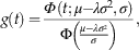
This model shows how a one phase model of loss filters the normally distributed trajectory generated by a single fluctuation in production (Fig. 6). If production over time follows a normal distribution with mean μ (i.e., the time of maximum production) and variance σ 2 (determined by the rate of increase and decrease in production), and the time to disintegration follows a one-phase model with loss rate λ, then the expected distribution of shells with ages > 0 years is equal to
 $$g(t)={{\iPhi \,(t;\mu {\minus}\lambda \sigma ^{2} ,\sigma )} \over {\Phi \left( {{{\mu {\minus}\lambda \sigma ^{2} } \over \sigma }} \right)}},$$
where Φ refers to the density for a normal distribution with mean μ t equal to μ−λσ 2 and with variance equal to σ 2, and Φ refers to the cumulative distribution function for a normal distribution with mean equal to 0 and variance equal to 1. The frequency distribution of shell ages thus follows a truncated-normal distribution (i.e., only positive shell ages are drawn from a normal distribution). The higher the loss rate (thin black lines in Fig. 6, as opposed to thin gray lines) and/or the lower the rate of decline in production (decreases from left to right in graphs of Fig. 6), then the larger the difference between the original production trajectory and the snapshot AFD, and between μ t and μ (Fig. 7). As loss rates increase and/or the rates of change in production decrease, the modes of AFDs will be shifted to younger age cohorts, causing the true timing of past production pulses to be underestimated (Fig. 6). High loss rates result in only the most recent part of the production pulse being captured by the death assemblage. Even when the mode in the AFD is younger than the true peak in production, the variance of its truncated-normal distribution is equal to variance in the trajectory in production, and so can be used to directly estimate the rate of increase or decrease in production.
Effects of shell loss and of rate of change in production on the timing of maximum past production. Assuming a one-phase model of loss, the difference between the true time of maximum production (i.e., mode of the original production trajectory) and the mean of the truncated-normal model estimated on the basis the AFD (i.e., mode of the AFD) increases with A, increasing loss rate (scenarios differing in standard deviation shaded in different colors) and B, increasing standard deviation of the original production trajectory (i.e., decreasing rate of change in production). The same two effects will also affect the difference between the true and apparent time of maximum production under a two-phase model of loss, but this difference will be reduced with increasing τ (time to attain SZ) and decreasing λ 2 (loss rate in SZ).
Two-Phase Truncated-Normal Model
This model shows how a two-phase model of loss affects the AFD generated by a single fluctuation in production. If the time to disintegration is a mixture of two phases of loss, then the expected distribution of postmortem ages is
 $$g(t)=\beta {{\iPhi \,(t;\mu {\minus}\lambda _{2} \sigma ^{2} ,\sigma )} \over {\Phi \left( {{{\mu {\minus}\lambda _{2} \sigma ^{2} } \over \sigma }} \right)}}{\plus}(1{\minus}\beta ){{\iPhi \,(t;\mu {\minus}({\rm \lambda }_{{\rm 1}} {\plus}\tau )\sigma ^{2} ,\sigma )} \over {\Phi \left( {{{\mu {\minus}({\rm \lambda }_{{\rm 1}} {\plus}\tau )\sigma ^{2} } \over \sigma }} \right)}}.$$
The distribution of postmortem ages is thus a mixture of two truncated-normal distributions, with means equal to μ t1=μ−(λ 1+τ) σ 2 and μ t2=μ−λ 2σ 2. Identical values of μ t1 and μ t2 imply that the difference between λ 1+τ and λ 2 is negligible, thus supporting the one-phase model rather than the two-phase model of loss. As in the one-phase model described above, the relationship between these means and the original time of maximum production μ depends on loss rates (determined by λ 1, τ, and λ 2) and on the magnitude of σ 2: both of these parameters shift μ t, and thus also the observed AFD mode, towards younger ages relative to the true timing of the production pulse (μ). The timing of maximum production μ can nonetheless be inferred by using a range of loss rates estimated at sites where shells are still being produced, i.e., where a key assumption of the loss-rate model is not violated.
In contrast to the effects of a one-phase model, the two-phase loss model can, under some circumstances, generate bimodal AFDs. The young mode is composed of shells still surviving from recent, post-pulse production, and the older mode is composed of shells surviving from the past pulse of production: sequestration in the SZ allows the relicts of past production pulses to persist in death assemblages even when an AFD is dominated by the youngest cohorts, which peak at ~0 age. This bimodality thus arises under conditions of high λ 1 and very low λ 2 (thereby minimizing the shift of the production pulse towards modern time), combined with an intermediate rate of change in production. At a very slow decline in production, only the recent production is preserved, whereas at a very rapid decline in production, only the past production pulse is preserved.
One-Phase and Two-Phase Models of Abrupt Increase and/or Termination in Production
The time of first colonization of a seafloor or landscape, for example determined by the flooding of an estuary or human introduction of an alien species, can lead to a rapid increase in production; a natural or anthropogenic disturbance can also result in an abrupt decline in production to zero levels. If the timing of first colonization T max and/or the timing of the termination in production T min can be estimated from independent data, then loss can be estimated by the addition of a prior probability that accounts for times with zero production, so that f(t)=0 for t<T min, t>T max, f(t)=1 for t≥T min, and t≤T max. The expected distribution of postmortem ages for one-phase model is
 $$g(t)=\left[ {{1 \over {{{\lambda _{{\rm 1}} \left( {e^{{{\minus}\lambda _{1} T_{{min}} }} {\minus}e^{{{\minus}\lambda _{1} T_{\vskip 1ptmax} }} } \right)} \over {\lambda _{1} }}}}} \right]^{n} .\mathop{\Pi }\limits_{{i=1}}^{n} \left[ {\lambda _{1} \,e^{{{\minus}\lambda _{1} t}} } \right].$$
The expected distribution of postmortem ages for two-phase model is
 $$\eqalignno{ g(t)=&\left[ {{1 \over {{{\tau (e^{{\minus}{\lambda_{2} T_{min} }} {\minus}e^{{{\minus\lambda _{2} T_{\vskip 1ptmax}{}} }} )} \over {\lambda _{2} }}{\plus}{{(\lambda _{1} {\minus}\lambda _{2} )(e^{{{\minus}(\tau {\plus}\lambda _{1} )T_{min} }} {\minus}e^{{{\minus}(\tau {\plus}\lambda _{1} )T_{{\vskip 1ptmax }} }} )} \over {\tau {\plus}\lambda _{1} }}}}} \right]^{n} \cr &\times \mathop{\prod}\limits_{{i=1}}^{n} [\tau e^{{{\minus}\lambda _{2} t}} {\plus}(\lambda _{1} {\minus}\lambda _{2} )e^{{{\minus}(\tau {\plus}\lambda _{1} )t}} ].$$
By adding to the model a prior probability that accounts for the absence of shells that are younger than T min (Fig. 4D), estimates of loss rate can be estimated with higher accuracy than those obtained from constant-production models (Fig. 4C).
AFDs from the Southern California Shelf
Onshore-Offshore Gradient in the Shape of AFDs
AFDs change markedly in their shape with increasing water depth. The median shell age increases from 21 y at 23–31 m, to 141 y at 40–48 m, 4778 y at 51–58 m, and 12,112 y at 89 m (Table 1). AFDs of the three shallowest assemblages show a L-shaped, hollow-curve distribution: they are dominated by shells <50 years old but possess long tails with shells as old as ~12,000 years (Fig. 8). The 51–58 -m assemblage has two modes, with a major mode at 100 years and a second more subtle mode at ~6,000 years, whereas the 89 m assemblage is rather unimodal, peaking at ~11,500 years (Fig. 8, Table 1). Thus with increasing water depth, the skew of the AFDs changes from positive to negative values. The age range in the three shallowest assemblages is as large as ~11,000–12,000 years, and that of the 89-m assemblage is 21,189 years. The onshore-offshore gradient in interquartile range (IQR) is less marked, with a smaller IQR in the two shallowest assemblages (2731 y and 3136 y) than in two deeper assemblages (6908 y and 4880 y).
A–D, Age-frequency distributions (AFDs) of shells of the bivalve Nuculana taphria in death assemblages sampled at four water depths on the Southern California continental shelf, based on amino acid racemization dating and calibrated in years before 2003 AD. With increasing water depth, median shell age increases and the skewness of AFDs decreases.
Median age, IQR, total age range, and skewness of age-frequency distributions (AFDs) of Nuculana taphria in four bathymetrically arrayed death assemblages from the southern California continental shelf. Median is in years before 2003 AD with bootstrapped 95% confidence intervals in parentheses. N=number of shells dated.
Model Fitting
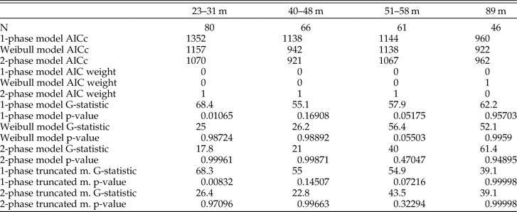
The two-phase model has an AIC weight equal to ~1 and thus outperforms both the Weibull and the one-phase models in explaining the shape of the AFDs of the three shallowest assemblages (Table 2; as also found with a larger array of AFDs in this region by Tomašových et al. Reference Tomašových, Kidwell, Foygel Barber and Kaufman2014). The two-phase model also does best at explaining these assemblages using a G-test and outperforms other models in predicting the median age and IQR of three shallowest assemblages (black points in Fig. 9A,B). However, the G-statistic of the assemblage at 51–58 m is not significantly different from the prediction of the two-phase truncated-normal model. This model clearly captures the bimodal shape of the AFD observed at this water depth, suggesting the fingerprints of a past production pulse here.
A, B, Comparison of median ages and interquartile ranges (IQR) observed in death assemblages and those predicted by five models of loss. In the three shallowest assemblages (from 23 to 58 m), both summary statistics are accurately predicted by a two-phase model (black circles): these predicted values lie closest to or on top of the diagonal line indicating equivalence with observed values. In contrast, the deepest assemblage (89 m; with median=12,113 years and IQR=4880 years) is best predicted by truncated-normal models (crosses and stars), indicating that production has not been constant. Some results plot on top of others so that not all 20 data points are visible. C, Estimates of loss rates λ 1 and λ 2 (black and gray circles, respectively) and of sequestration rate τ (white circles) for AFDs along a bathymetric gradient (with bootstrapped 95%confidence intervals). Even though the shapes of AFDs change markedly with increasing water depth (x-axis), each parameter remains fairly constant along the bathymetric gradient, with λ 1 and λ 2 differing consistently by two orders of magnitude.
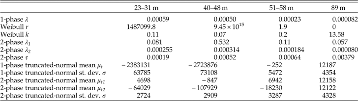
Estimated parameters of three models with constant production and two models with varying production (see explanation in text).
In contrast, based on AIC, the Weibull model outperforms a two-phase model in the deepest, 89-m assemblage, where it predicts a rather uniform right-censored distribution with k=13.6. When k > 1, the Weibull function can generate unimodal and even left-skewed non-censored distributions because shells degrade at a higher rate as they age. However, such a dynamic cannot generate a left-skewed right-censored distribution. Based on the G-statistic, the deepest assemblage is best supported by both of the truncated-normal models that allow production to vary, and the expected distributions of these models do not differ significantly from the AFD observed at 89 m (Table 2). Truncated-normal models also predict the median age and IQR of the deepest assemblage fairly accurately (stars in Fig. 9A,B).
Estimates of Disintegration and Sequestration
In the three shallowest assemblages (23–58 m), λ 1 varies between 0.076 and 0.53 (corresponding to decadal to yearly half-lives, or a annual loss of 7 and 41% of shells in a cohort, Table 3) and is two orders of magnitude larger than λ 2, which varies between 0.00018 and 0.00031 (half-lives of ~3900 to 2200 years, or annual loss of 1.7 and 3%). τ ranges between 0.00019 and 0.00064, which correspond to the median time to sequestration (stabilization or burial) falling between ~3650 and 1100 years. The variables τ and λ 1 are independent and thus, even when τ is much smaller than λ 1, some shells can still be sequestered during the first few decades (e.g., about six out of 1000 shells at τ=0.00064), even when they represent a minor proportion of the original production.
Goodness of fit with AIC weights and the G-statistic for three constant-production models and two truncated-normal models that allow production to vary. The three shallowest assemblages are best supported by a two-phase model on the basis of AIC weights and G-test. The assemblage from 89 m has stronger support from both truncated-normal models.
The Weibull model also outperforms a one-phase model in shallow assemblages, and its very low shape parameter (k=0.09–0.20) implies a similar, markedly rapid temporal decline in loss rates. The baseline rate parameter r of the Weibull model is extremely high (106–1015), but likelihood surfaces of the Weibull model (1) yield a very broad range of rate estimates with very similar log-likelihood values, and (2) show a negative correlation between the estimates of r and k. In contrast, log-likelihood surfaces show that two-phase model parameter estimates are uncorrelated and have relatively steep log-likelihood surfaces (Supplementary Figure 1). The parameters of the Weibull models are thus less precise compared to the estimates of two-phase models. In spite of the increase in median shell age and IQR from 23 to 58 m (Table 1), the two-phase model parameters detects a two order-of-magnitude decline in loss rates in each of the three shallow-water assemblages, and yields water depth-invariant estimates of λ 1, τ, and λ 2 across most of the shelf transect (Fig. 9C).
Estimates of Past Changes in Production
AFDs that are better fit by constant production models can nonetheless still originate under variable production because the signature of a change in production is essentially removed by high loss rates and/or by slow rates of change in production. Thus, when estimating the timing of a past change in production, we focus both on the 89 m assemblage and on the 51–58-m assemblage: the latter is better supported by a two-phase model with constant production, but appears to be bimodal as predicted by the two-phase truncated-normal model, with the second mode at ~6000 years. The two-phase truncated-normal model shows that the standard deviation of the original normal distribution is ~3287 years for the 51–58 m assemblage and ~4328 years for the 89 m assemblage: that is, in both water depths, the rise and decline in production occurred on a millennial scale. The estimated means of the truncated-normal distributions are ~6942 years ago for the 51–58-m assemblage and ~12,100 years ago for the 89-m assemblage (slightly older than the observed mode of that distribution at 11,591 years). We use (1) the loss rates estimated from the two-phase models and (2) estimates of μ and σ 2 from the two-phase truncated-normal models to compute the timing of maximum production μ (i.e., the mean of the normal distribution) for assemblages at 51–58 m (gray lines in Fig. 10) and at 89 m (black lines in Fig. 10): the two-phase dynamic is best supported at the shallow sites with active production. Using the range of loss rates estimated from all four assemblages, the timing of maximum production was ~7800–10,300 years ago for 51–58 m (Fig. 10C) and ~13,650–18,050 years ago for 89 m (Fig. 10D).
Inferring the timing of maximum production based on AFDs from two water depths (51–58 m and 89 m), assuming that the change in production follows a normal distribution trajectory. In A, we use the probability densities of the two-phase model estimated from all four assemblages because they are rather depth-invariant (Fig. 8C). B, The truncated-normal models fitted to the 51–58 m (gray line) and 89 m (black line) assemblages. C, D, the inferred production trajectories at 51–58 m and 89 m, where the means of the distributions are determined from the four two-phase densities in A and from the fits of the truncated-normal models in B. The standard deviations are determined from the fits of the truncated-normal models in B. Past pulses in production (sets of thick lines in C, D) occurred a few thousand years earlier (arrow) than would be suggested by the modes of the observed truncated-normal distributions (faint dashed line shows fit as determined in B).
Discussion
Mechanisms of Disintegration and Sequestration
The shallowest death assemblages with active production of Nuculana taphria shells in southern California, that is those assemblages collected from seafloors within the preferred 19–56 meter depth range of this species, all possess right-skewed AFDs that are better supported by models assuming constant production than models assuming variable production. In these assemblages, our analysis gives the strongest support to models that imply a very high disintegration rate (decadal half-lives), such as commonly measured during bench and field experiments, followed by a slow long-term disintegration rate and/or slow net burial rates below the mixed layer (millennial half-lives) that can explain the large window of time averaging. The rapid decline in loss rate experienced by shells as they age can be conceptualized as the threshold between significantly different preservation regimes. For intrinsically fragile shell types (such as very thin and/or organic-rich shells), a fast-track to the SZ via burial may well be the only successful route for long-term carbonate preservation: this can be achieved if the TAZ is very thin, or if large-scale burial events are frequent, e.g. via downward advection by burrowers or thick storm deposits (e.g., Aller Reference Aller1982). Refuge in the SZ can also be achieved in sediments where the probability of diagenetic stabilization increases abruptly across short physical distances, for example from incomplete bioturbation that permits pockets of saturated or supersaturated pore waters near the sediment-water interface. While in those pockets, we postulate diagenetic stabilization, for example from intercrystalline cementation and coatings (Perry Reference Perry1999; Rivers et al. Reference Rivers, James and Kyser2008; Jarochowska 2012), annealing (coarsening of microstructure) in the absence of mineralogical change (Walter and Morse 1984; Morse and Casey Reference Morse and Casey1988; Hu and Burdige Reference Hu and Burdige2007), and/or recrystallization of aragonite or high-Mg calcite to thermodynamically more stable minerals (Reid and Macintyre Reference Reid and Macintyre1998; Brachert and Dullo Reference Brachert and Dullo2000; Hover et al. 2001). Any of these processes might reduce the likelihood of disintegration during reworking. “Safety in numbers”, whereby a primary concentration of shells benefits by self-buffering of porewaters and/or by resisting erosional reworking, might also contribute (e.g., Seilacher Reference Seilacher1985; Kidwell Reference Kidwell1989), as might bioencrustation and bioimmuration. These diverse mechanisms are not mutually exclusive, and all have been invoked, singly or in combination, to explain the ‘paradox of preservation’ of diverse skeletal carbonates, especially aragonite, under conditions of low net seafloor aggradation, although burial is usually favored (e.g., Kidwell 1985, Reference Kidwell1989; Davies et al. Reference Davies, Powell and Stanton1989). Preliminary SEM analyses imply that N. taphria shells only a few thousands years old show coalescence of original crystallites, suggesting that the decline in loss rates is related to microstructural changes.
The two-phase model does not explicitly disentangle burial of shells downward from exhumation of shells upward (from the SZ into the TAZ). If sequestration (movement to a SZ) is coupled with burial (greater sediment depth below the depositional interface), τ can correspond to a simple burial rate (in the absence of exhumation) or to a net burial rate when burial events are counteracted by exhumation events. When partitioning of λ 1 and λ 2 is generated by vertical separation of TAZ and SZ rather than by horizontal heterogeneities, two-phase models can conceptualize the AFD of a death assemblage sampled by gear that bites down into (1) at least some portion of the SZ (Fig. 2D) or (2) into the TAZ only, but where that TAZ has received shells reworked upward after some period experiencing low rates of loss in a SZ (Fig. 2E).
In situations where (1) the sampled death assemblage derives entirely from the uppermost part of the seabed, presumably just the TAZ, and yet (2) the empirical data support a two-phase exponential model, then (3) the estimate of λ 2 indicates that shells were in fact reworked up from the SZ to the TAZ. At least two natural scenarios are possible. In the first, shells are diagenetically stabilized irreversibly during their residence in the SZ, and thus keep their slow loss rates λ 2 after they move back to the TAZ (Fig. 2E). In the second, shells revert to fast disintegration rates λ 1 when they are reworked back into the TAZ (Fig. 2D). They are older than other shells in the TAZ because they had a “time-out” from those fast loss rates but, once back in the TAZ, they resume disintegrating as fast as younger shells there. In this second scenario, λ 2 in the SZ will be underestimated relative to its true values. Both scenarios produce a set of shells within the TAZ that are much older than they would have been had they spent their entire postmortem existence within the TAZ. They can be thus expected to produce a strongly right-skewed and long tailed, characteristically L-shaped AFD within the TAZ.
Sampling designs with stratified depth of burial, presently underway on the southern California shelf by us (2-cm core increments) and elsewhere by others, will be needed to detect whether old shells (1) derive from deeper parts of the mixed layer corresponding to the SZ, and/or (2) represent shells reworked upward from the SZ. On the basis of bone-age data from a series of fully buried and well-stratified small-mammal assemblages, Terry and Novak (Reference Terry and Novak2015) suggest that disintegration rates can be biased upward (i.e., inferred rates will be erroneously high) if skeletal hardparts are not completely mixed within the top sediment layer because hardparts reworked downward would be more frequent than those reworked upward. This situation would arise from a down-core decline in hardpart abundance under constant disintegration; and would increase the slope of an AFD. Their cave-hosted record contrasts with the marine conditions considered here. On the southern California shelf, as elsewhere, biological processes mix sediment at monthly, yearly, and decadal scales that are rapid relative to centennial or millennial scales of long term burial rates (e.g., Alexander and Lee Reference Alexander and Lee2009). Our models thus assume that the TAZ and SZ are vertically or horizontally separated but internally well mixed.
The Dynamic of Production
With increasing water depth, southern California AFDs of N. taphria become less skewed, unimodal, and better supported by models with temporally variable production. The variance of the truncated-normal distribution implies a millennial-scale decline in production. This millennial-scale offset is almost certainly linked to N. taphria tracking its preferred shallow-water habitat with post-glacial rise in sea level. The onshore-offshore gradient in the shapes of AFDs is thus driven by a gradient in the timing of active production, with earlier onset and earlier shutdown of production in deeper environments. This conclusion is supported by our finding that estimates of disintegration and sequestration do not change markedly with water depth (Fig. 9C). Based on data for live-collected bivalves in the Southern California Bight, the proportional abundance of living N. taphria peaks between 19 and 56 m (Fig. 11). Death assemblages from 89 m depth on the modern shelf are thus presently out of the depth range preferred by N. taphria, and the assemblages at 51–58 m are on the outer edge of preferred water depths.
Timing in the production of Nuculana taphria found in death assemblages at 51–58 m and 89 m water depth on the present-day southern California shelf. Left graph: Based on sampling of living macrobenthos on the shelf (2003–2004), N. taphria has peak abundances at shallow depths, with the 5th and 95th percentiles between 19 and 56 m. Right graph: Based on the two-phase truncated-normal models fitted to AFDs from our two depth zones, maximum production occurred ~7800–10,300 years ago at the 51–58 m sites and 13,650–18,050 years ago at the 89 m sites (gray bands, based on Fig. 10C,D). The brackets on these time-frames of maximum production are based on the minima and maxima of loss rates of the two-phase model (vertical dashed lines). These estimates are in good agreement with the independent sea-level curve of Nardin et al. (Reference Nardin, Osborne, Bottjer and Scheidemann1981) for southern California, which is reproduced here to show the history of deepening at these two sites. Our 51–58 m depth zone (thick black line is its water depth trajectory) supported a water column 19–56 m deep between 0 and 11 ka, and the 89 m depth zone (thick gray line) supported the preferred water depths ~12.5 ka to 17.5 ka. At the times of maximum production estimated from the AFDs, the estimated water depths at these two depth zones were thus within the preferred depth range of N. taphria (horizontal dashed lines) at the times of maximum production estimated from the AFDs.
Based on the two-phase truncated-normal models of the AFDs at these two sites (Fig. 10C–D), maximum production at the 51–58 m sites is estimated at ~7800–10,300 years ago and maximum production at the 89 m sites is estimated to have occurred 13,650–18,050 years ago (intervals denoted by gray bands in right-hand graph of Fig. 11). These estimates of maximum production derived from AFDs are in good agreement with the independent sea-level curve of Nardin et al. (Reference Nardin, Osborne, Bottjer and Scheidemann1981) for southern California. At the times of maximum production estimated from AFDs, the water depths of these sites were indeed within the preferred depth range of N. taphria (horizontal dashed lines)—the 51–58 m sites were 19–56 m deep between 0 and 11 ka (thick black line is the water depth trajectory), and the 89 m sites were in that depth range ~12.5 ka to 17.5 ka (thick gray line). Although sea-level change since the last glacial maximum on the southern California shelf remains poorly constrained, the estimated times and depths of maximum production are comparable to the preferred depth of Nuculana taphria. Similar migrations of species producing local population declines can be predicted for other species on continental shelves, along with analogous shifts in latitude and, on land, altitude with climate change.
Conclusions and Implications
Our new models demonstrate for the first time the joint effects of skeletal loss and variable production on the postmortem age-frequency distributions (AFDs) of death assemblages sampled in the mixed layer, and thus show how these key variables can be reconstructed, using molluscan shell assemblages from the southern California shelf.
First, when interpreting the timing of a past peak in production or the timing of a recent decline, such as for conservation and historical ecology studies, it should be expected that high loss rates and slow declines in production have pulled the modes of AFDs forward toward a more modern time. These factors will also tend to modify unimodal trajectories of production (symmetrical pulses) into right-skewed AFDs, with the result that those AFDs might be better fitted by constant-production models even though production was declining over the course of time averaging. Care thus must be exercised, but these biases are predictable in direction magnitude. Specifically, they underestimate the timing of production pulses.
Second, where populations were extirpated or their production declined strongly, loss rates inferred from AFDs will approximate the long-term rates of disintegration within the mixed layer and/or the rates of burial below the mixed layer, and thus the true rates of recycling in the taphonomically active zone will be underestimated. In the absence of recently produced shells, the AFD cannot detect the short-term, initially high loss rates such as would be detected in short-term experimental deployments of shells.
Finally, we find from our field test that, although AFD shapes vary across the southern California shelf, with increasing median shell age and age range and loss of skew with water depth, estimated rates of disintegration and sequestration do not change. The cross-shelf gradient in time averaging is thus created by a gradient in the timing of production (here, the transgressive migration of our target species with sea-level rise) rather than by gradients in disintegration and burial rates. Regardless of water depth, most shells in the mixed layer disintegrate quickly, with decadal-scale half-lives, whereas a small subset of shells persist for millennia by attaining a refuge from high loss rates. This postmortem persistence permits death assemblages sampled at local scales to carry information on composition and diversity accrued over long temporal scales, permitting the capture of regional-scale composition (Warme Reference Warme1969; Kowalewski et al. Reference Kowalewski, Goodfriend and Flessa1998; Smith Reference Smith2008; Tomašových and Kidwell Reference Tomašových and Kidwell2010; Miller et al. Reference Miller, Behrensmeyer, Du, Lyons, Patterson, Toth, Villasenor, Kanga and Reed2014; Hassan Reference Hassan2015) even when most shells disintegrate quickly. This consistency in dynamics across the shelf, derived from AFD data, is also encouraging for habitat-scale paleoecological inference: it suggests that bathymetric variation in live-dead agreement in species composition that is encountered in some meta-analyses (e.g., Kidwell 2001; Tomašových and Kidwell 2011) arises from differences in scales of time averaging (and thus environmental condensation) rather than from bias per se (interspecies differences in preservation), a distinction that has not previously been possible.
Acknowledgments
We thank A. Ranasinghe of the Southern California Coastal Water Research Project for arranging release of sieve residues from the Bight’03 survey; R. Velarde, D. Cadien, and T. Parker for helpful insights into the Southern California Bight system; D. S. Kaufman of Northern Arizona University for AAR analyses; the NOSAMS facility in Woods Hole for radiocarbon analyses; and for funding the University of Southern California Sea Grant Program (National Oceanic and Atmospheric Administration), the National Science Foundation (EAR-0345897 and EAR-1124189), the Slovak Research and Development Agency (APVV 0644-10), and the Slovak Scientific Grant Agency (VEGA 0136-15). We thank an anonymous reviewer for helpful comments, T. D. Olszewski for a review and help with a graphical presentation of censoring effects, and M. Foote for raising the issue of censoring at the beginning of our project.
Supplementary Material
Supplemental materials deposited at Dryad: doi: 10.5061/dryad.rv0k6