1. Introduction
Owing to their abundance in scientific and engineering applications, wall-bounded flows have been a key area in turbulence research. Initially, the focus centred on the near-wall region owing to its direct relation to the generation of skin friction. Over the last couple of decades, however, the focus has shifted towards the logarithmic layer, partly because advancements in experimental technique and numerical computing have enabled access to flow databases with a sufficiently resolved logarithmic layer. Yet, a more fundamental reason for the interest in the logarithmic layer is that it is of great importance in the large-scale applications of high-Reynolds-number wall-bounded turbulence (such as large transportation devices). For instance, the amount of bulk turbulent kinetic energy (TKE) production and dissipation within the logarithmic layer (Marusic, Mathis & Hutchins Reference Marusic, Mathis and Hutchins2010; Jiménez Reference Jiménez2018) and the contributions to the skin friction from the flow structures residing in the logarithmic layer (de Giovanetti, Hwang & Choi Reference de Giovanetti, Hwang and Choi2016) both increase with increasing Reynolds number.
One way of investigating the intrinsic dynamics of a particular subregion of the flow is to isolate it from the rest of the flow. In wall-bounded turbulence, one of the prime examples is the minimal flow unit of Jiménez & Moin (Reference Jiménez and Moin1991). They were able to isolate a quasi-cyclic sequence of a single set of flow structures in the buffer layer by systematically restricting the simulation domain, which shed light on its intrinsic dynamics. Flores & Jiménez (Reference Flores and Jiménez2010) extended this approach to the logarithmic layer and identified a series of restricted minimal domains in which turbulence characteristics are well-replicated up to a wall-normal distance proportional to the spanwise domain size. They used them to study the characteristics of a hierarchy of the minimal logarithmic layer structures without an influence from the large-scale outer layer motions. Later, Hwang (Reference Hwang2015) combined this method with an overdamped large eddy simulation (LES) (use of an intentionally elevated value of eddy viscosity to damp out the small-scale motions; see Hwang & Cossu Reference Hwang and Cossu2010) to isolate flow structures of a given step in the hierarchy. Based on this experiment, he concluded that the flow structures at each hierarchy can sustain themselves. However, there is still a question of whether overdamping simply filters out the small-scale motions (without affecting the large-scale motions) or modifies the dynamics of the whole flow by effectively reducing the Reynolds number (Feldmann & Avila Reference Feldmann and Avila2018).
Whereas the previous examples attempt to isolate structures of certain sizes or locations, the study of statistically stationary homogeneous shear turbulence (SSHST) takes the different approach of isolating a particular element of the logarithmic layer, namely the shear. Unlike experimental homogeneous shear flows, where the size of the structures grows indefinitely, a statistically stationary state is achieved numerically by using a limited spanwise flow domain (e.g. Pumir Reference Pumir1996; Sekimoto, Dong & Jiménez Reference Sekimoto, Dong and Jiménez2016). This flow setup lacks near-wall dynamics, and is hence suitable for investigating the isolated effect of the mean shear on the flow dynamics. Dong et al. (Reference Dong, Lozano-Durán, Sekimoto and Jiménez2017) conducted an extensive study of the coherent structures in SSHST, and concluded that its structures are essentially symmetrised and unconstrained (by the wall) versions of the structures in turbulent channels, which suggests that the shear is the main ingredient of the coherent structure dynamics in the logarithmic layer. However, SSHST is still not equivalent to the logarithmic layer because it cannot replicate the wall-normal dependence of the characteristic length scale or the inhomogeneity along the wall-normal direction.
In this regard, a closer reproduction of the logarithmic layer is the numerical experiment by Mizuno & Jiménez (Reference Mizuno and Jiménez2013) where the buffer layer (as well as the wall itself) was removed and substituted by an off-wall boundary condition. They introduced the scale variation along the wall-normal direction by using a rescaled interior plane as the off-wall boundary (without the rescaling, the resulting flow was very similar to SSHST). Their numerical experiment reproduced many characteristics of the natural logarithmic layer, albeit not perfectly. For example, a spurious ‘buffer layer’ formed near the off-wall boundary owing to the formation of small-scale vortices caused by the incoherence between the off-wall boundary and the adjacent flow. Alternatively, Lozano-Durán & Bae (Reference Lozano-Durán and Bae2019) achieved the same objective by using slip and permeable boundary conditions. This experiment reproduces the outer layer dynamics of the no-slip channel well but only does so above some adaptation height, which is of the order of the slip length applied for the boundary conditions. In combination with that, Bae & Lozano-Durán (Reference Bae and Lozano-Durán2019) used a minimal spanwise domain to remove the large-scale outer layer structures to isolate the logarithmic layer.
All the aforementioned studies were successful at replicating or isolating certain features of the logarithmic layer, but also had some drawbacks which made them incompatible with the natural flow. In the previous attempts to isolate the logarithmic layer of turbulent channel flows, there have been numerous strategies for removing the buffer layer dynamics. However, to the best of the authors’ knowledge, the removal of the outer layer large-scale structures has relied almost exclusively on the use of a minimal spanwise domain. In this work, an alternative strategy is employed to remove the large-scale outer motions by modifying the driving force of the flow. It has an advantage that the large-scale structures are removed without artificially saturating their wall-parallel growth. This method is somewhat similar to the method of Jiménez & Pinelli (Reference Jiménez and Pinelli1999) where they introduced an explicit damping term in the evolution equations of the flow above the buffer layer to remove the outer layer motions. The resulting flow had a laminar outer flow while the undisturbed part of the flow displayed similar behaviour to the near-wall turbulence, although some of the flow statistics were altered. However, in the present work, the evolution equations of the flow are not modified except by the body force. Therefore, this investigation aims to isolate the logarithmic layer of turbulent channel flows with a minimal disturbance to its essential dynamics.
As in most of the examples just mentioned, the system that we analyse here is only an approximation to the canonical logarithmic layer. As in those cases, it is best understood as an example of the ‘thought experiments’ that have been a mainstay of physics for a long time. The system is intended to represent the logarithmic layer in the same sense that point masses are often used to represent planets. In all these cases, it is equally important to recognise which features are retained by the approximation and which are not. We show in the following that some properties that could be expected to depend on the near-wall region (e.g.the self-similar hierarchy of attached eddies) are well-reproduced by our approximation, even if that region is missing from our model. However, properties linked to the outer flow are not well-reproduced, and this will be used to explain the origin of some of the features observed in true logarithmic layers. It is also important to emphasise that the logarithmic layer requires a theory that cannot simply be provided by increasing the Reynolds number of the simulations. In intermediate asymptotic ranges, such as the logarithmic layer or the inertial range of isotropic turbulence, the theory for the self-similar regime requires being able to separate its dynamics from the details of its interactions with the inner and outer limits (Barenblatt Reference Barenblatt1996). Nonetheless, those details are often important in themselves. For example, the interaction of the logarithmic layer with the near-wall layer is key to formulating correct boundary conditions for large-eddy simulations (Jiménez & Moser Reference Jiménez and Moser2000), whereas the interaction with the outer flow is required to understand why and how properties such as the turbulence intensities depend on the Reynolds number (Hutchins & Marusic Reference Hutchins and Marusic2007).
The organisation of this paper is the following. § 2 outlines the details of the numerical experiments and § 3 assesses the quality of the isolated logarithmic layer. Finally, the major findings of this paper are discussed in § 4 with the conclusions presented in § 5.
2. Numerical experiment
For this investigation, turbulent flow between two parallel plates, separated by the distance  $2h$, was simulated at a nominal
 $Re_\tau =hU_\tau /\nu =2000$, where
 $\nu$ is the kinematic viscosity of the fluid and
 $U_\tau$ is the friction velocity. Periodic boundary conditions were used along the wall-parallel directions and no-slip and impermeable boundary conditions were applied at both walls. Throughout the paper, the streamwise, wall-normal and spanwise coordinates are denoted by
 $x$,
 $y$ and
 $z$, respectively, and the corresponding velocity components by
 $U$,
 $V$ and
 $W$. The
 $y$-dependent ensemble-averaged quantities are represented by an overline, whereas lowercase velocity variables indicate fluctuations with respect to this average (e.g.
 $U=\bar {U}+u$). A ‘
 $+$’ superscript indicates normalisation by the viscous scale
 $\nu /U_\tau$ for length and by
 $U_\tau$ for velocity. The domain length in
 $x$ and
 $z$ are
 $L_x=2{\rm \pi} h$ and
 $L_z={\rm \pi} h$, respectively, to make sure that the entire flow domain is not minimal in the wall-parallel directions (Flores & Jiménez Reference Flores and Jiménez2010). The flow was simulated via LES with a static Smagorinsky sub-grid scale (SGS) model (Smargorinsky Reference Smargorinsky1963). The Smagorinsky constant was chosen to be
 $C_s=0.1$, and the statistics of the LES compared well with a direct numerical simulation (DNS) database at the same Reynolds number. The computational algorithm and the numerical code were taken from those employed in Vela-Martín et al. (Reference Vela-Martín, Encinar, García-Gutiérrez and Jiménez2019), but adapted for LES. The code solves the wall-normal vorticity and the Laplacian of
 $v$ formulation of the Navier–Stokes equations (Kim, Moin & Moser Reference Kim, Moin and Moser1987). Along the wall-parallel directions, the equations were projected onto Fourier basis functions along a uniform mesh. A non-uniform mesh was used in the wall-normal direction to account for the inhomogeneity in that direction, and the wall-normal gradients were computed by using seven-point compact finite differences with spectral-like resolution (Lele Reference Lele1992). For temporal integration, a low-storage semi-implicit third-order Runge–Kutta scheme was used (Spalart, Moser & Rogers Reference Spalart, Moser and Rogers1991).
Because the purpose of the current experiment is to isolate the dynamics of the logarithmic layer, it has to adequately resolve the energy-containing motions in that region. For this purpose, a DNS database of channel flow at the comparable  $Re_\tau$ (Hoyas & Jiménez Reference Hoyas and Jiménez2006, hereafter referred to as HJ06) was examined as a benchmark, and it was found that more than
 $95\,\%$ of the total turbulent kinetic energy,
 $k=(\overline {u^2}+\overline {v^2}+\overline {w^2})/2$ was contained within motions whose streamwise and spanwise wavelengths were larger than 74 viscous length units for
 $y^+>100$. Therefore, the nominal grid spacings in
 $x$ and
 $z$ were chosen to be
 ${\rm \Delta} x^+={\rm \Delta} z^+\simeq 37$, after de-aliasing. In the wall-normal direction, the grid was defined by a hyperbolic tangent stretch function such that the
 $n$th grid location is given by
 $y_n/h=\tanh [3(n-1)/511-3/2]/\tanh (3/2)+1$ for
 $n=1,2,\ldots ,512$, between the lower wall at
 $y=0$ and the upper wall at
 $y=2h$. The parameters of the simulations are summarised in table 1. Here,
 $Re_\tau$ for LW, LWc and LN are given based on
 $U_\tau$ from the extrapolated total shear stress at the wall to highlight the agreement of the total stress profile within the linear-stress layer. However, it does not carry the usual meaning of the ‘Reynolds number’ for the canonical channel flows because the scale separation and the wall-normal gradient of the total shear stress become independent parameters for our isolated layers (for the canonical channel flows, they are both related by
 $Re_\tau$).
Simulation parameters for the numerical experiments and for the reference DNS database. Here,  ${\rm \Delta}$ represents the grid spacing in each direction. The grid spacings in the wall-parallel directions are calculated after dropping 1/3 of the high-wavenumber modes for de-aliasing. The LES cases include the base case (LB), the main experiment with a wider logarithmic layer (LW), the supplementary experiment with a narrower logarithmic layer (LN) and the experiment with a constant stress profile (LWc). For LW, LWc and LN,
 $U_\tau$ is computed by extrapolating the total shear stress to the wall. For LWc,
 $h$ is the wall-normal simulation domain. The next-to-last column shows the total time over which the statistics are gathered, in terms of the large-eddy turnover time (
 $h/U_\tau$).

To validate this numerical methodology, the base LES (case LB) was first conducted and compared against HJ06. For this case, a van Driest damping function of the form  $D(y^+) = [1-\exp (-y^+/26)]^2$ was used on the Smagorinsky eddy viscosity to enforce the zero SGS stress conditions at the wall. Figure 1 shows the profiles of the mean streamwise velocity
 $\bar {U}$ and of the second-order velocity statistics of LB. The primed velocity variables indicate the root-mean-square (RMS) value. A good agreement was observed between the statistics of LB and HJ06. Although not shown here for brevity, the one-dimensional velocity spectra also showed a good agreement. Throughout the paper, further statistical comparisons will be made where appropriate to demonstrate that our LES code reproduces well the logarithmic layer of turbulent channel flows.
(a) Mean streamwise velocity: solid line, LB; dashed line, HJ06. (b) Second-order velocity statistics:  $\rhd$,
 $u'^+$;
 $\triangle$,
 $v'^+$;
 $\circ$,
 $w'^+$;
 $\square$,
 $\overline {uv}^+$; solid lines with closed symbols, LB; dashed lines with open symbols, HJ06.

Several methods were tested to isolate the logarithmic layer by removing the turbulent fluctuations outside it. The initial strategy was to employ an elevated value of  $C_s$ outside the logarithmic layer (i.e. overdamped LES; see Hwang & Cossu Reference Hwang and Cossu2010) and its effect on the flow was investigated by varying the value of
 $C_s$ in the usual buffer layer (
 $y^+<70$). However, with increasing
 $C_s$ near the wall, it was observed that the spectral signature of the near-wall cycle gradually moved outwards instead of being eliminated at a fixed location (see the Appendix).
Hence, instead of damping previously created turbulent fluctuations, an alternative approach is sought where the necessity of ‘active’ turbulent fluctuations is eliminated outside the logarithmic layer. This is achieved by setting a prescribed total mean shear stress (sum of viscous, Reynolds and SGS stresses) profile which drops to zero outside the nominal logarithmic layer. In practice, this is done by imposing a modified profile of the body force. This method is found to be effective at eliminating the buffer layer, and was chosen as our preferred method for isolating the logarithmic layer. The method of modifying the stress profile also means that the elimination of the outer layer dynamics can be achieved without relying on the restricted flow domain and hence allows us to investigate its effects on the large-scale structures, which is not possible in the case of the minimal logarithmic layer experiments where the large-scale structures are, by construction, truncated. In fact, the idea is not new. For example, Tuerke & Jiménez (Reference Tuerke and Jiménez2013) simulated turbulent channel flows with a prescribed mean velocity profile to study its effects on the dynamics of energy containing eddies, and Borrell (Reference Borrell2015) applied an extra body force to model the effects of roughness near the wall. It is also known that a modified body force can lead to laminarisation of the flow at transitional Reynolds numbers (He, He & Seddighi Reference He, He and Seddighi2016; Kühnen et al. Reference Kühnen, Song, Scarselli, Budanur, Riedl, Willis, Avila and Hof2018). Russo & Luchini (Reference Russo and Luchini2016) investigated the linear response of the mean streamwise velocity of turbulent channel flows to a body force, albeit at low Reynolds number. However, to the best of our knowledge, this method has not been used for the purpose of isolating a particular subregion of the flow.
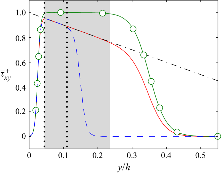
Two numerical experiments were performed with different prescribed mean stress profiles, as shown below and in figure 2,
 \begin{equation} \bar{\tau}_{xy} = \frac{U_\tau^2}{4}(1-y/h)\left(1+\tanh[\beta_l(y/h-y_l/h)]\right)(1-\tanh[\beta_u(y/h-y_u/h)]). \end{equation}
This equation is defined for  $0 \leq y \leq h$, but the prescribed stress profile was extended to the opposite side of the channel using symmetry. The parameters
 $y_l$ and
 $\beta _l$ control the location and width of the region where the stress profile decays from its natural value to zero between the nominal logarithmic layer and the wall. Likewise,
 $y_u$ and
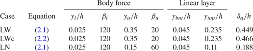
 $\beta _u$ control the location and width of the region where the stress profile decays smoothly to zero above the nominal logarithmic layer. The parameters for the stress profiles for the main experiment with an isolated logarithmic layer (case LW) and for the supplementary experiment with a narrower log layer (case LN) are given in table 2. The values of
 $y_l$,
 $\beta _l$,
 $y_u$ and
 $\beta _u$ are set empirically.
Profiles of the mean shear stress. The lines are as indicated in table 1, except for the dashed-dotted line,  $\bar {\tau }_{xy}^+=1-y/h$ (LW, LWc and LN are presented by red, green and blue colours, respectively). The linear-stress layer for LW and LWc is indicated by the grey shaded area and that for LN is indicated by the vertical dotted lines.

Parameters for the prescribed stress profiles. The linear-stress layer is the region where the deviation from the natural stress profile ( $\bar {\tau }_{xy}^+=1-y/h$ for LW and LN, and
 $\bar {\tau }_{xy}^+=1$ for LWc) is below
 $1\,\%$. Here
 $\delta _a$ represents the height of the active stress region where
 $\bar {\tau }_{xy}^+>0.01$.

In addition to the cases of LW and LN, another experiment was performed in which the prescribed stress profile was constant within the isolated layer. This intended to mimic the total stress profile in the logarithmic layer as the streamwise pressure gradient vanished. For this experiment, referred to as LWc, the prescribed stress profile is
 \begin{equation} \bar{\tau}_{xy} = \frac{U_\tau^2}{4}\left(1+\tanh[\beta_l(y/h-y_l/h)]\right)(1-\tanh[\beta_u(y/h-y_u/h)]), \end{equation}
which only differed from (2.1) by the missing  $(1-y/h)$ factor. The parameters
 $y_l$,
 $\beta _l$,
 $y_u$ and
 $\beta _u$ were kept as in LW to study the effect of changing the stress profile independently from other factors. In conventional channel flows, the channel centreline provides a natural symmetry plane for the total stress profile (i.e.
 $\bar {\tau }_{xy}=0$). This does not apply to LWc, where the extrapolated location of zero mean shear stress would be infinitely far from the wall. Therefore, the upper wall of LWc was replaced by a free-slip impermeable boundary at
 $y=h$ (
 $\partial u/\partial y=\partial w/\partial y=0$ and
 $v=0$). Although physically not required, fine grid spacing is needed near the free-slip wall to numerically enforce the boundary conditions (in particular, to numerically resolve exponential functions with large exponents for high wavenumbers). Hence, a different wall-normal grid was used for LWc, such that the
 $n$th grid location is given by
 $y_n/h=\tanh [3(n-1)/383-3/2]/(2\tanh (3/2))+1/2$ for
 $n=1,2,\ldots ,384$ for
 $0\leq y_n\leq h$. This grid was designed such that the wall-normal spacing was kept similar to that used for LB, LW and LN within the domain of interest (
 $0.05\lesssim y/h\lesssim 0.2$). It should be noted that
 $h$ simply means the wall-normal domain size for LWc, not the channel half height.
We defined the ‘linear-stress’, or ‘active’, layer to be the region in which the prescribed shear-stress profile deviates by less than  $1\,\%$ from the natural stress profile in channels with an unmodified body force (i.e.
 $\bar {\tau }_{xy}^+=1-y/h$ for LW and LN, and
 $\bar {\tau }_{xy}^+=1$ for LWc). While eddies within this layer could be expected to be ‘most natural’, taller eddies have to exist up to the level at which some tangential stress must be carried by the flow. We therefore also introduced a length scale,
 $\delta _a$, intended to be indicative of the height of the largest momentum-transferring eddies, defined as the point at which
 $\bar {\tau }_{xy}^+=0.01$ (approximately
 $1\,\%$ of the wall shear stress in the natural channel). The limits
 $y_{bot} < y < y_{top}$ of the linear layer and
 $\delta _a$ of the active layer are given in table 2. Note that although
 $y_{top}$ and
 $\delta _a$ are related, they are independent parameters, whose ratio can be changed by modifying the stress profile. Both will be used below to scale different quantities, but, because
 $y_{top}/\delta _a\approx 0.5$–0.6 in all our experiments, it is impossible to say which of the two, if any, was the most physically relevant scale. However, it follows from the definition of
 $\delta _a$ that we can tentatively assign
 $\delta _a=h$ in unmodified channels.
Within the linear-stress layer, the flow experiences a body force equivalent to that generated by the mean pressure gradient in a canonical channel, and most of the stress is carried by the Reynolds stress. For example, the flow in LN and LW has to produce the same mean momentum flux as in a natural channel at  $Re_\tau =2000$, and could therefore be expected to have the same dynamics as the logarithmic layer in such a channel. For LWc, no driving body force is present in the linear region, and the flow is maintained by the localised body forces applied above and below the linear-stress layer. For the actual numerical computation, the stress profile was enforced by replacing the mean pressure gradient in the mean streamwise momentum equation with
 $-{\rm d} \bar {\tau }_{xy}/{\rm d} y$. No van Driest damping was used, because the buffer layer was outside the domain of validity of the experiments, and there was no need to reproduce its behaviour. Figure 2 shows the actual stress profiles for LW, LWc and LN, which followed the prescribed profiles well. For all the numerical experiments in which the wall shear stress was intentionally modified, the effective
 $U_\tau$ was estimated by extrapolating the stress in the linear-stress layer to the wall. This was the velocity scale used for normalisation in table 1.
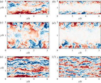
As a preliminary result and a qualitative comparison, instantaneous snapshots of the field of  $u$ for LB and LW are shown in figure 3. They demonstrate that the turbulent fluctuations in the centre of the channel were eliminated in LW. This was also true in the buffer layer, although they were too small to be observed visually. Within the isolated layer, the turbulent structures were qualitatively similar in both cases, although it is noteworthy that streaks whose streamwise length was comparable to the streamwise domain were observed in LB but not in LW. This difference will be further investigated by the spectral analysis in § 3.2.
Instantaneous fields of  $u$ for: (a,c,e) LB; (b,d,f) LW. The wall-parallel planes in (e,f) are at
 $y/h=0.15$. The colours range from
 $u=-4U_\tau$ (dark blue) to
 $4U_\tau$ (dark red).

3. Assessment of the isolated logarithmic layer
3.1. One-point statistics
In this section, we examine whether the flow in an isolated linear-stress layer can replicate the characteristics of the natural logarithmic layer by comparing the statistics of the truncated cases, LN and LW, with those of the full channel LB. In addition to that, we examine the effects of changing the stress profile by comparing case LW with LWc, which is intended to represent the limiting case of the channel flow without the driving force. Figure 4(a) shows the profiles of the mean streamwise velocity. Note that because the walls were outside the domain of validity of the three isolated cases, the no-slip condition did not provide an absolute velocity reference, and a Galilean offset of the profile is required in general (Mizuno & Jiménez Reference Mizuno and Jiménez2013). In fact, it is clear from the figure that the mean velocity of the truncated layers vanished below  $y^+\approx 60$ (and actually became slightly negative). Much of the effect of the no-slip condition was taken over by the dragging effect of the body force, and the profiles for LW, LWc and LN needed to be shifted by
 $15U_\tau$ to be comparable to the canonical logarithmic layer. The agreement of the mean velocity after this shift was fair within the active layer, but the velocity gradient became steeper as the linear-stress layer became narrower. This is further examined in figure 4(b), which tested the mixing length,
 $l_m=U_\tau /S$, where
 $S={\rm d} \bar {U}/{\rm d} y$. For a logarithmic mean velocity,
 $l_m^+ (y^+)$ is a linear function whose slope is the Kármán constant, but the mixing-length profile of LW, LWc and LN is not linear, even within the active layer. By comparing wall-bounded flows with different geometries (with the exception of Ekman layers), Johnstone, Coleman & Spalart (Reference Johnstone, Coleman and Spalart2010) and Luchini (Reference Luchini2017) found that in the logarithmic and outer layers, the negative streamwise pressure gradient induces a positive shift in the mean streamwise velocity, and vice versa. In our experiments, the mean streamwise velocity of LWc was higher than that of LW, which seems to be contradictory to the previous results. However, a direct comparison was not possible here because a positive shift in the
 $\bar {U}$ profile of LWc with respect to LW was caused by the difference in the wall-normal profile of the body force, rather than by the geometry or pressure gradient. Although the total integrated force must sum to zero in both LW and LWc, the magnitudes of integrated positive and negative forces (i.e. the difference between the minimum and maximum
 $\bar {\tau }_{xy}$) were approximately
 $5\,\%$ larger in LWc, which resulted in a greater amount of mean shear and the positive shift in
 $\bar {U}$.
(a) Mean streamwise velocity (shifted by  $15U_\tau$ for LW, LWc and LN). (b) Mixing length. For LW, LWc and LN, only the linear shear stress region is shown. The lines are as indicated in table 1 (LB, LW, LWc and LN are presented by black, red, green and blue colours, respectively). The linear-stress layer for LW and LWc is indicated by the grey shaded area and that for LN is indicated by vertical dotted lines.

The difference in the mean velocity was further investigated by comparing the mean shear profiles of the four LES cases. Figure 5(a) shows that they collapsed poorly when  $S$ was normalised by
 $U_\tau$ and
 $h$. However, in our experiments,
 $h$ did not convey the usual meaning of an outer length scale, because the eddies of height
 $h$ were purposely suppressed. Instead, we propose that the alternative length scale,
 $\delta _a$, was more relevant to the physics of the flow, because it represents the height of the tallest momentum-transferring eddies. Figure 5(b) shows that the profiles collapsed well within the linear-stress layer when both
 $S$ and
 $y$ were normalised with
 $\delta _a$, at least up to
 $y\simeq 0.4\delta _a$. It was particularly interesting that the profile of the mean shear scaled with
 $\delta _a$ even when the profile of total shear stress (which also represents the driving force) changed within the active layer, such as between LW and LWc. This suggests that the value of shear within the logarithmic layer is associated with, or possibly decided by, the size of the largest active eddies in the flow, and that this size is controlled by
 $\delta _a$. Moreover, the fact that the profiles agree within the active layer, when properly scaled, suggests that the truncated flows contain a self-similar eddy hierarchy, as in the natural logarithmic layer, although the range of sizes within the hierarchy may differ.
Mean shear profile scaled by (a) the channel half height; (b) the width of active stress layer. The lines are as indicated in table 1 (LB, LW, LWc and LN are presented by black, red, green and blue colours, respectively). The linear-stress layer for LW and LWc is indicated by the grey shaded area and that for LN is indicated by vertical dotted lines.

Figure 6 compares the Reynolds stress profiles of the four LES cases. All the stresses decayed for  $y\gtrsim 2\delta _a$, and figure 6(d) shows that the shear stress agreed well within the active layer for LB, LW and LN, as expected from the design of the experiment. An important observation was the absence of a buffer-layer
 $u'$ peak in LW, LWc and LN, which suggests that the buffer-layer dynamics had been suppressed. There were some residual velocity fluctuations below the linear-stress layer, but they were not involved in the net momentum transfer or in TKE production, because they only carried a negligible fraction of the tangential Reynolds stress (i.e. they were inactive, see figure 6d). The shape of the
 $u'$ profiles within the linear-stress layer was similar for LB, LW and LN, but their amplitude decreased as the width of the active layer decreased. The same decreasing trend was observed for
 $w'$ when comparing LW and LN, and we will argue below that both trends resulted from the attenuation of the large-scale fluctuations by the restricted height of the active layer. Here, the effects of changing the height of the active layer was solely attributed to the change in the scale separation within the eddy hierarchy, because LB, LW and LN shared the same mean shear stress within the linear-stress layer. In contrast, the value of
 $v'$ was slightly higher for LW and LN than for LB. The exact reason for this is not clear, but the most likely explanation was that an elevated
 $v'$ is required to compensate for the missing tangential Reynolds stress that used to be contributed by the large-scale
 $u$-eddies that would otherwise have originated above the active region (see figure 3). In the outer part of the flow, where
 $y\sim \mathcal {O}(\delta _a)$, the profiles of the truncated simulations collapsed well when
 $y$ was scaled with
 $\delta _a$ (not shown), which indicated that they had similar outer layer dynamics.
Profiles of (a)  $u'^+$, (b)
 $v'^+$, (c)
 $w'^+$ and (d)
 $-\overline {uv}^+$. The lines are as indicated in table 1 (LB, LW, LWc and LN are presented by black, red, green and blue colours, respectively). The linear-stress layer for LW and LWc is indicated by the grey shaded area and that for LN is indicated by vertical dotted lines.

The RMS velocity fluctuations in LWc were stronger than in LW. This was expected, because previous investigations of channel flows with altered stress profiles (Tuerke & Jiménez Reference Tuerke and Jiménez2013; Lozano-Durán & Bae Reference Lozano-Durán and Bae2019) have concluded that the magnitude of the fluctuations within the logarithmic layer scales with the local value of tangential Reynolds stress, and because the primary role of turbulent fluctuations in the logarithmic layer is to carry the tangential Reynolds stress required for the transfer of momentum. To check this, the RMS velocity profiles are shown in figure 7 scaled with the local velocity scale  $u^*=(-\overline {uv})^{1/2}$. Figure 7(d) confirms that it is indeed true that most of the mean shear stress was carried by
 $-\overline {uv}$ within the linear-stress layer, as in the logarithmic layer of natural flows. The profiles of LW and LWc now agreed well, but the consistent decrease with decreasing
 $\delta _a$ remained, especially for
 $u'/u^*$. Note that figure 7 includes profiles from the DNS channel by del Álamo et al. (Reference del Álamo, Jiménez, Zandonade and Moser2004), whose
 $h^+=934$ is comparable to the
 $\delta _a^+$ of LW and LWc. The three flows agreed reasonably well.
Profiles of (a)  $u'$, (b)
 $v'$, (c)
 $w'$ and (d)
 $-\overline {uv}$ normalised by (a–c)
 $u^*=(-\overline {uv})^{1/2}$ and (d)
 $\bar {\tau }_{xy}$. The lines are as indicated in table 1 (LB, LW, LWc and LN are presented by black, red, green and blue colours, respectively). In (a–c), solid lines with triangles are the
 $Re_\tau =934$ channel by del Álamo et al. (Reference del Álamo, Jiménez, Zandonade and Moser2004). The linear-stress layer for LW and LWc is indicated by the grey shaded area and that for LN is indicated by vertical dotted lines. The vertical scale is kept as in figure 6 to facilitate comparison.

We therefore turned our attention to the effect of  $\delta _a^+$, and plotted in figure 8 the average value over
 $100 < y^+ < 200$ of the TKEs of the three velocity components as functions of
 $\delta _a^+$ for the different DNS databases and LES experiments. The averaging range was chosen to be within the active or logarithmic layer in all the datasets included, and we set
 $\delta _a=h$ for the DNS databases. In all cases, the TKEs were normalised with the local
 $\overline {uv}$. For the DNS databases,
 $\overline {u^2}$ and
 $\overline {w^2}$ displayed a log-linear trend with respect to
 $h^+$, whereas
 $\overline {v^2}$ stayed roughly constant. This was consistent with the predictions from the attached eddy hypothesis (Perry & Abell Reference Perry and Abell1977; Perry & Chong Reference Perry and Chong1982), in which the main effect of increasing
 $h^+$ was considered to be to extend the range of scales of the self-similar attached eddy hierarchy. The results from the LES experiments (solid symbols) agreed well with the trend of the DNS databases, except for a slight
 $\overline {w^2}$ excess for LW and LWc, which arose from the mild hump in their
 $w'$ profile within the linear-stress layer (figure 7c). In addition to reinforcing the importance of
 $\delta _a$ as a parameter, this agreement supported the equivalence of
 $\delta _a$ and
 $h$ in natural channels, which suggests that the active part of the largest Townsend-type self-similar attached eddies reaches the channel centreline, even though they are obscured in that region by the presence of wake structures (see also del Álamo et al. Reference del Álamo, Jiménez, Zandonade and Moser2006; Lozano-Durán, Flores & Jiménez Reference Lozano-Durán, Flores and Jiménez2012). Another implication of this result is that the level of TKE in the logarithmic layer is almost exclusively determined by the scale separation among the self-similar momentum-transferring eddies, whereas the Reynolds shear stress provides the velocity scale. Therefore, for the isolated layers,
 $\delta _a$ acts as a control parameter that determines the scale separation as well as the mean shear as a function of
 $y/\delta _a$ (figure 5b), and
 $\delta _a$ is an independent parameter from the shear stress gradient, unlike natural channel flows. This is made especially clear by the agreement between LW, LWc and del Álamo et al. (Reference del Álamo, Jiménez, Zandonade and Moser2004) despite having different mean Reynolds shear stress gradients and driving forces. Such comparisons are not possible in natural channel flows because the scale separation within the self-similar attached eddies and the mean stress gradient both depend on the Reynolds number.
TKE of each velocity component normalised by the local  $\overline {uv}$ averaged over
 $100 < y^+ < 200$:
 $\rhd$,
 $\overline {u^2}/{-\overline {uv}}$;
 $\triangle$,
 $\overline {v^2}/{-\overline {uv}}$;
 $\circ$,
 $\overline {w^2}/{-\overline {uv}}$. Open symbols connected with solid lines represent DNS databases at
 $Re_\tau =547$ (del Álamo & Jiménez Reference del Álamo and Jiménez2003), 934 (del Álamo et al. Reference del Álamo, Jiménez, Zandonade and Moser2004), 2004 (HJ06), 4179 (Lozano-Durán & Jiménez Reference Lozano-Durán and Jiménez2014) and 5181 (Lee & Moser Reference Lee and Moser2015). Solid symbols represent LES experiments LB (black), LW (red), LWc (green) and LN (blue).

3.2. Spectra
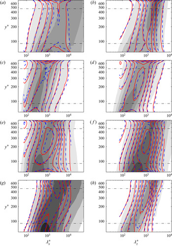
To examine the distribution of turbulent kinetic energy at different scales, one-dimensional premultiplied spectra are plotted in figure 9. All the spectra were suppressed outside the linear-stress layer, but the most notable observation was the elimination of the near-wall spectral peak in the spectrum of  $u$ for LW and LN, which is especially clear in figure 9(b) and proved that our numerical experiment effectively removed the dynamics of the buffer layer. Another important difference was the attenuation, within the linear-stress layer of LW and LN, of the spectrum of
 $u$ at very large
 $\lambda _x$ and
 $\lambda _z$. The motions in this range of wavelengths are commonly referred to as the very large-scale motions (VLSMs) of the logarithmic layer (e.g. Jiménez Reference Jiménez1998; Kim & Adrian Reference Kim and Adrian1999) and some attention has been dedicated to them, because they carry a substantial fraction of the TKE and of the Reynolds stresses (Balakumar & Adrian Reference Balakumar and Adrian2007). However, the present result suggests that the VLSMs are not part of the intrinsic dynamics of the logarithmic layer, but of the region above it, which has been suppressed by the body force in LN and LW. This idea is consistent with the concepts of ‘inertial waves’ in Jiménez (Reference Jiménez2018) or of ‘global modes’ in del Álamo & Jiménez (Reference del Álamo and Jiménez2003), introduced to describe the energetic motions of
 $u$ at very large wavelengths which occupy the majority of the channel half width. Kwon (Reference Kwon2016) tried a different way of eliminating the outer layer contributions to the velocity fluctuations from the perspective of the quiescent core. He observed that, upon the removal of the velocity fluctuations associated with the quiescent core, most of the energy of
 $u$ in the VLSM range disappears.
One-dimensional pre-multiplied spectral density of (a,b)  $u^2$, (c,d)
 $v^2$, (e,f)
 $w^2$ and (g,h)
 $-uv$ along the (a,c,e,g) streamwise and (b,d,f,h) spanwise directions. The grey shaded contours are for HJ06, solid contours are for LW and dashed contours are for LN. Contour lines are drawn at multiples of
 $0.1U_\tau ^2$ except for (a) 0.2; (b) 0.4; (g) 0.05. The horizontal dashed-dotted lines are
 $y/h=0.045$,
 $0.11$ and
 $0.235$, and mark the boundaries of the linear-stress layer for LW and LN.

The damping of the long and wide wavelengths in LN and LW is made explicit in figure 10, which shows the difference between their spectra and the full LES case. The restricted layers exhibited an energy deficit with respect to LB, and this was restricted to the large scales. Moreover, the length of the region in which LN fell below LB (e.g.  $\lambda _x^+\approx 3500$ at the
 $0.1U_\tau ^2$ level of
 $k_x\phi _{uu}$ in figure 10a) was approximately twice as short than for LW, proportionally to their respective
 $\delta _a$. The width of the spanwise defect followed a similar trend but the peak was located at
 $\lambda _z \approx h$ in both cases, which is consistent with the known width of the VLSM (Jiménez Reference Jiménez2018). Note that there are no plots for
 $\phi _{vv}$ in figure 10. This velocity component had no VLSM and the corresponding plots were almost empty.
Difference between the one-dimensional pre-multiplied spectral density of (a,b)  $u^2$, (c,d)
 $w^2$ and (e,f)
 $-uv$ along the (a,c,e) streamwise and (b,d,f) spanwise directions. The grey shaded contours are LB-LW and line contours are for LB-LN. In (a) the contours are separated by
 $0.1 U_\tau ^2$, in (b) the contours are separated by
 $0.2 U_\tau ^2$ and in (c–f) the contours are separated by
 $0.05 U_\tau ^2$. The horizontal lines are the limits for the two linear-stress layers.

All these studies converged to the conclusion that the VLSMs do not belong to the self-similar wall-attached eddy hierarchy intrinsic to the logarithmic layer. This is not to say that they have no influence on its dynamics, but suggests that the origin and dynamics of the VLSMs are associated with the outer layer rather than with the logarithmic layer. A similar attenuation of the large scales was observed for  $w$ and, to a lesser degree, for
 $uv$, but not for
 $v$, consistent with Reference TownsendTownsend's (Reference Townsend1976) idea that the
 $u$ and
 $w$ fluctuations are attached, in the sense that they are created far from the wall and extend downwards to fill the space underneath, while the
 $v$ fluctuations are local in
 $y$. This is also clear from the triangular spectral ‘skirts’ in figures 9(a,b) and 9(e,f). The lack of skirts in figures 9(c,d) and 9(g,h) shows that these roots are ‘inactive’ with respect to the tangential stress. It is interesting to observe the dependence of the large-scale energy attenuation on the thickness of the linear-stress layer, which is demonstrated by the greater attenuation in LN compared with LW. This supports the idea that restricting the wall-normal dimension over which turbulent fluctuations can develop also limits their growth in the wall-parallel directions. Long structures at a given
 $y$ are the skirts of structures farther up, and truncating the top of the spectral triangle also truncates the long wavelengths. Therefore, the structures in the linear-stress layer are ‘minimal’ in the wall-normal direction, and the upper bound of the linear-stress layer acts as a ‘ceiling’ that limits the growth of the structures in the wall-parallel directions as well. This also explains the decreasing trend of
 $u'$ and
 $w'$ with decreasing
 $\delta _a$ shown in figure 8.
Figure 11 presents two-dimensional velocity spectra at three wall-normal locations to examine the self-similarity of the velocity fluctuations in the isolated linear-stress layer, which is the defining characteristic of natural logarithmic layers. For brevity, only LW and LB are compared in the figure, but LN and LWc displayed a similar collapse. The wavelengths were scaled with the local mixing length, which was shown by Mizuno & Jiménez (Reference Mizuno and Jiménez2011) to collapse the velocity spectra in DNS channels better than the distance from the wall. More recently, Lozano-Durán & Bae (Reference Lozano-Durán and Bae2019) proposed a similar length scale, also based on the mean shear but using the local velocity scale  $\overline {-uv}^{1/2}$ instead of
 $U_\tau$, but the difference between the two scales is small for the range of wall-normal locations in figure 11, and we have kept the traditional definition. The energetic cores of the spectra of LW at different wall-normal locations showed an excellent collapse, which supported the conclusion that the mixing length is the correct length scale for the energy-containing eddies in the logarithmic layer, even when the profile of the mixing length is not linear. If the typical velocity scale within the logarithmic layer is given by
 $U_\tau$, this implies that the time scale of the energy-containing eddies is dictated by the local mean shear rather than by a local eddy turnover based on the distance from the wall and
 $U_\tau$. The core of the spectra of LW also agreed well with LB. The lack of collapse at the large-scale ends of
 $k_xk_z\phi _{uu}$ and
 $k_xk_z\phi _{ww}$ was already discussed in figure 9, and corresponds to the inactive structures, which scale with
 $h$ or with
 $\delta _a$. In particular, note the damping of the spectrum of LW in the upper-right corner of figure 11(a,d).
Contour plots of (a)  $k_xk_z\phi _{uu}$, (b)
 $k_xk_z\phi _{vv}$, (c)
 $k_xk_z\phi _{ww}$ and (d)
 ${-}k_xk_z\phi _{uv}$ against
 $\lambda _x/l_m$ and
 $\lambda _z/l_m$, scaled by the mixing length at each height. The solid greyscale contours are for LW and computed at
 $y/h\simeq 0.1$, 0.15 and 0.2 (from light grey to black). The dashed colour contours are for LB and computed at
 $y/h\simeq 0.1$ (blue),
 $0.15$ (red) and
 $0.2$ (green). Contour levels are drawn at (a)
 $[0.1\ 0.3]U_\tau ^2$, (b,d)
 $[0.03\ 0.1]U_\tau ^2$ and (c)
 $[0.05\ 0.15]U_\tau ^2$.

Figure 12 examines the effect of changing the stress profile in layers of similar thickness by comparing the cases LW and LWc. The one-dimensional spectra were normalised with  $u^*$, which was shown in the previous section to be the correct scale for the intensities, and shown only within the linear-stress layer. They collapsed well, showing that the spectral distribution of the fluctuations, and not only their TKE, was independent of the existence of a pressure gradient.
One-dimensional pre-multiplied spectral density of (a,b)  $u^2$, (c,d)
 $v^2$, (e,f)
 $w^2$ and (g,h)
 $-uv$ along the (a,c,e,g) streamwise and (b,d,f,h) spanwise directions. The grey shaded contours are for HJ06, solid contours are for LW and dashed contours are for LWc. Contour lines are drawn at multiples of
 $0.1u^{*2}$ except for (a) 0.2; (b) 0.4; (g) 0.05. The horizontal dashed-dotted lines indicate
 $y=0.045h$ and
 $0.235h$, which mark the boundaries of linear-stress layers.

To complement the observations on the trend of the large-scale energy attenuation, figure 13 compares two-dimensional energy spectra at  $y/h\simeq 0.1$, scaled with
 $u^*$. The spectra for the full LES (LB) agreed well with HJ06, again demonstrating the adequacy of the current LES simulations for the study of the logarithmic layer. There was some accumulation of energy at the scales close to the grid resolution of LES, owing to the slightly insufficient dissipation by the SGS model, but this effect did not extend to the energy-containing region. The spectra for LW and LWc agreed well, which reinforced the conclusions from the one-dimensional data. The comparison between LB, LW and LN clearly showed the removal of large-scale energy as the width of the linear-stress layer decreased, especially for
 $u$ and
 $w$. This also explained the previously observed decreasing trend of the
 $u'$ and
 $w'$ profiles with decreasing
 $\delta _a^+$, discussed in figure 6.
Contour plots of (a)  $k_xk_z\phi _{uu}$, (b)
 $k_xk_z\phi _{vv}$, (c)
 $k_xk_z\phi _{ww}$ and (d)
 ${-}k_xk_z\phi _{uv}$ at
 $y\simeq 0.1h$ plotted against
 $\lambda _x/l_m$ and
 $\lambda _z/l_m$. The shaded contours are HJ06. The line contours are LES experiments as indicated in table 1 (LB, LW, LWc and LN are presented by black, red, green and blue colours, respectively). Contour levels are drawn at (a)
 $[0.1\ 0.3]u^{*2}$, (b,d)
 $[0.03\ 0.1]u^{*2}$ and (c)
 $[0.05\ 0.15]u^{*2}$. The black dashed diagonal lines represent
 $\lambda _x=\lambda _z$.

However, there was a TKE excess in the spectra of all the restricted-layer experiments with respect to LB and HJ06, at the intermediate scales, which can be observed in figures 11 and 13. The wavelengths of the excess energy in the LW scale, with the mixing length above  $y/h=0.075\ (y^+=150)$, were centred around
 $(\lambda _x,\lambda _z) \simeq (15l_m,10l_m)$ for
 $v$ and
 $w$, and around
 $(\lambda _x,\lambda _z) \simeq (30l_m,10l_m)$ for
 $u$. This energy excess also produced some extra Reynolds shear stress, which appeared as an upper ‘horn’ in figure 13(d). This extra Reynolds shear stress was needed to compensate for the attenuated Reynolds shear stress at the large scales. The same energy excess also appeared in LN, where it was stronger because it had to compensate for an even larger attenuation. Except for these localised effects, the agreement in the other regions of the two-dimensional spectra was very good.
There was also an energy excess in the wide modes of  $v$ in LN, which can be observed in figure 13(b), and which also appeared in LW near the lower limit of the linear-stress layer (not shown). Because its wavelengths were wide and relatively short, it was tempting to attribute this extra energy to a spanwise instability of the shear layer that formed underneath the linear-stress region (see the peak at
 $y^+\approx 70$ in figure 5). The extra energy in the near-wall region is also visible in figure 9(a,b) as a ‘stem’ at
 $\lambda _x^+\approx 700$ and
 $\lambda _z^+\approx 2000\text {--}3000$, hanging below the spectrum of LW into the near-wall damped layer. It can also be shown that the spectrum of
 $u$ at
 $y^+=20$, although weak overall, contained very wide structures with
 $\lambda _x^+\approx 700$. Note that these wavelengths were much wider in the spanwise direction than any residual near-wall peak that might have not been fully damped by the forcing. Jiménez et al. (Reference Jiménez, Uhlmann, Pinelli and Kawahara2001) showed that any profile with an approximate inflexion point near the wall developed a Kelvin–Helmholtz like instability as soon as any amount of wall transpiration was allowed. García-Mayoral & Jiménez (Reference García-Mayoral and Jiménez2011) showed that, in ribbed surfaces modelled by a layer of retarding body forces, this effect results in transverse unstable rolls. This instability, like Kelvin–Helmholtz's, is essentially inviscid and depends only on the mean
 $u$ profile and on the
 $v$ velocity that separates the inflection point from the impermeable wall. Its typical wavelengths are of the order of 5 to 10 times the thickness of the drag layer, which in the present case of
 $(\lambda _x^+\approx 450\text {--}900)$ would not be too far from the observed values. In the case of the ribbed surface mentioned above, the effect of the instability is mostly confined to the damped layer. However, in our cases, there was another shear layer above the linear-stress layer, so there could be a resonance between two shear layer instabilities located below and above the linear-stress layer, which may act as a seeding mechanism for the energy excess within the isolated layer. To confirm this possibility is beyond the scope of the present paper, but the direct influence of the possible instabilities does not seem to be significant, and the characteristics of the energy-containing eddies are well-reproduced.
3.3. Dynamic indicators of the flow
Examination of velocity statistics reveals that our numerical experiment was able to replicate key kinematic properties of the natural logarithmic layer. To further assess the resemblance of the linear-stress layer to the natural logarithmic layer, we also examined and compared some of the dynamic characteristics of the flow. First, we examined the ratio between the production and dissipation of TKE, because it is widely known that these two quantities are approximately in balance in the logarithmic layer. For LES channel flows, the balance of the mean TKE of the filtered velocity fields is given by
 \begin{equation} \frac{Dk}{Dt} = P+\epsilon+\varPi_p+\varPi_t+\varPi_v+\varPi_r, \end{equation}
where the terms on the right-hand side represent production, dissipation, pressure transport, turbulent transport, viscous diffusion and diffusion by residual stress, respectively. They are defined as
 \begin{gather} P ={-}S\overline{uv}, \end{gather}
 \begin{gather}\epsilon ={-}\overline{\boldsymbol{\tau^v}\boldsymbol{:}\boldsymbol{\mathsf{E}}}+\overline{\boldsymbol{\tau^r}\boldsymbol{:}\boldsymbol{\mathsf{E}}}, \end{gather}
 \begin{gather}\varPi_p ={-}\frac{\partial\overline{vp}}{\partial y}, \end{gather}
 \begin{gather}\varPi_t ={-}\frac{\partial\overline{vk}}{\partial y}, \end{gather}
 \begin{gather}\varPi_v = \nabla \boldsymbol{\cdot} \overline{\boldsymbol{u}\boldsymbol{\cdot}\boldsymbol{\tau^v}}, \end{gather}
 \begin{gather}\varPi_r ={-}\nabla \boldsymbol{\cdot} \overline{\boldsymbol{u}\boldsymbol{\cdot}\boldsymbol{\tau^r}}, \end{gather}
where  $\boldsymbol {u}$ is the fluctuating velocity vector
 $(u,v,w)$,
 $p$ is the kinematic pressure,
 $\boldsymbol{\mathsf{E}}$ is the strain rate tensor of the filtered velocity fields,
 $\boldsymbol {\tau ^v}=2\nu \boldsymbol{\mathsf{E}}$ is the viscous stress tensor and
 $\boldsymbol {\tau ^r}=-2\nu _r\boldsymbol{\mathsf{E}}$ is the residual stress tensor, where
 $\nu _r$ is the LES eddy viscosity given by the SGS model.
Another key parameter for characterising the dynamics of shear flow is the Corrsin parameter, which is defined as the ratio between the dissipative time scale of eddies ( $2k/\epsilon$) and the time scale of the mean shear (
 $1/S$). Therefore, it represents the relative importance of shear to the dynamics of turbulent eddies. For example,
 $2kS/\epsilon \gg 1$ means that the structures live long enough to experience the effects of the shear. Figure 14 shows the plots of the production/dissipation ratio and the Corrsin parameter for all the LES cases and for HJ06. The two full channels, LB and HJ06, showed some discrepancies below
 $y^+\simeq 100$, but agreed reasonably well above that level, which demonstrated the adequacy of our LES scheme for studying the logarithmic layer. For these two flows,
 $P/\epsilon \simeq 1$ over a wide range of wall-normal locations corresponding to the conventional logarithmic layer. The two isolated layers LW and LWc have a narrower region in which the deviation of the
 $P/\epsilon$ profile with respect to LB remains less than
 $5\,\%$, located in
 $200\lesssim y^+\lesssim 390$ (
 $0.1\lesssim y/h\lesssim 0.195$). However, the
 $P/\epsilon$ ratio never reaches unity in LN, presumably because the linear-stress layer is too narrow to fully recover the TKE balance. In the middle of the linear-stress layer, the Corrsin parameter in figure 14(b) agrees well among all of the LES cases and HJ06, and stays approximately constant at
 $2kS/\epsilon \approx 8.$ This agreement suggests that similar dynamic processes take place in all these flows. These observations demonstrate that our numerical experiments are able to produce a region whose dynamic characteristics are similar to those of the natural logarithmic layer.
(a) Ratio between production and dissipation. (b) Corrsin parameter. The lines are as indicated in table 1 (LB, LW, LWc and LN are presented by black, red, green and blue colours, respectively). The linear-stress layer for LW and LWc is indicated by the grey shaded area and that for LN is indicated by vertical dotted lines.

However, the profiles of  $P/\epsilon$ and of the Corrsin parameter for LW have peaks at
 $y^+\simeq 70$ and
 $y^+\simeq 570$ in figure 14, which are just outside of the linear-stress layer. This could potentially be worrying because the excess
 $P/\epsilon$ in these regions may influence the dynamics of the linear-stress layer. To investigate this possibility, figure 15 compares the actual production and dissipation profiles. When
 $P$ and
 $\epsilon$ were premultiplied by
 $y$ in figure 15(a) to highlight the logarithmic and outer regions, they did not agree well, even within the linear-stress layer. However, we saw in the previous section that the correct length scale for this region was the mixing length, and when the production was premultiplied by
 $l_m$ in figure 15(b), LW, LN and LB agreed excellently, while LWc did not. This was essentially automatic, because
 $l_m^+P^+=-\overline {uv}^+$, which was set by the body force, and whose profile was only different for LWc. The behaviour of
 $l_m^+\epsilon ^+$ was more interesting. The agreement between LB and LW near
 $y^+\simeq 280$ was consistent with the collapse of
 $l_m^+P^+$ and of
 $P/\epsilon$ in this region, but it is clear from figure 15(b) that the peaks of
 $P/\epsilon$ near the edge of the linear layer were caused by a reduced level of dissipation, not by an increased level of production. The balance of the two quantities was never reached for LN, because its linear-stress layer was too narrow (the scale separation between the two edges was only a factor of two). Tuerke & Jiménez (Reference Tuerke and Jiménez2013) investigated a turbulent channel flow with a sharp change in the mean shear, and found that the production adapts to the change in the shear almost immediately, while the dissipation does so more gradually, in agreement with the behaviour near the edges of the linear-stress layer in figure 15(b). They attributed this phenomenon to the temporal delay between the production and dissipation mechanisms.
Profiles of production and dissipation. Lines on the positive and negatives sides represent the production and dissipation, respectively: (a) premultiplied by  $y$ and (b) premultiplied by
 $l_m$. The lines are as indicated in table 1 (LB, LW, LWc and LN are presented by black, red, green and blue colours, respectively). The linear-stress layer for LW and LWc is indicated by the grey shaded area and that for LN is indicated by vertical dotted lines. In (b), profiles for LW and LWc are plotted only near the vicinity of the linear-stress layer (
 $70 < y^+ < 600$).

To further inspect this behaviour, the wall-normal flux of the mean TKE was considered. The transport terms in (3.1) are in the form of a flux divergence, and the wall-normal flux of the mean TKE,  $\varTheta$, can be computed as
 \begin{equation} \varTheta(y)=\int_{0}^{y}\left(\varPi_p(\xi)+\varPi_t(\xi)+\varPi_v(\xi)+\varPi_r(\xi)\right){\rm d} \xi . \end{equation}
As per (3.1), regions with positive  ${\rm d} \varTheta /{\rm d} y$ (i.e. positive transport) indicate net energy sinks,
 $\epsilon >P$, which draw energy from other wall-normal locations and vice versa. Also, because (3.8) vanishes at the wall, a positive
 $\varTheta$ indicates a net TKE flux towards the wall at that wall-normal location. Figure 16 shows
 $\varTheta$ for the LES cases and HJ06 (Hoyas & Jiménez Reference Hoyas and Jiménez2008). LW, LWc and LN agreed well below the linear-stress layer but LN did not exhibit a plateau region because it never recovered the local TKE balance. LW, LWc, LB and HJ06 exhibited a mild plateau region within the linear-stress or logarithmic layer but they only approximately agreed in the upper half of the linear-stress layer. The slope of
 $\varTheta$ in the logarithmic and linear-stress layers was negative, because
 $P/\epsilon$ was slightly greater than unity there (at least up to
 $Re_\tau =5200$; see Bernardini, Pirozzoli & Orlandi Reference Bernardini, Pirozzoli and Orlandi2014; Lee & Moser Reference Lee and Moser2015). Otherwise,
 $\varTheta$ had a positive slope at
 $y^+<55$ and
 $y^+>645$ for LW, which indicated that the flow acted as an energy sink outside of the linear-stress layer, except in the vicinity of the layer edges. In full channels, like LB and HJ06, the buffer layer (
 $5 < y^+ < 40$) acted as a strong energy source owing to the intense production activities. However, the removal of the buffer layer in LW turned this region into a net energy sink, whose energy deficit was balanced by an energy flux coming from the linear-stress layer. The region above
 $y^+\simeq 645$ also acted as a net energy sink and drew energy from the linear-stress layer. In LW and LWc,
 $\varTheta$ crossed zero at
 $y^+\simeq 125$, which meant that the TKE was transported towards the wall at
 $y^+<125$ and towards the centre at
 $y^+>125$. On average, some of the TKE produced in the linear-stress layer was transported away from the layer instead of being dissipated within it. This is different from the behaviour of natural logarithmic layers and explains the reduced level of dissipation near the edge of the linear-stress layer. For
 $200 < y^+ < 400$, the slope of
 $\varTheta$ in LW approached that of LB and HJ06, while the actual magnitude of TKE flux was smaller because there was less upward TKE flux coming from below. This region coincided with the location where a good agreement was observed for
 $P/\epsilon$ and the Corrsin parameter between LW, LWc and LB. Overall, the shear production mechanism of the logarithmic layer was well-reproduced in the linear-stress layer, although there were some differences in how the TKE was transported and dissipated near the layer edges. Therefore, the current numerical experiment is an adequate reproduction of the natural logarithmic layer as far as the energy producing and energy containing motions are concerned.
Profiles of the wall-normal TKE flux. The lines are as indicated in table 1 (LB, LW, LWc and LN are presented by black, red, green and blue colours, respectively). The linear-stress layer for LW and LWc is indicated by the grey shaded area and that for LN is indicated by vertical dotted lines.

4. Discussion
To isolate the logarithmic layer of wall-bounded turbulent flows, we have presented a series of numerical experiments in which a body force is used to impose a prescribed total stress profile. The resulting flow has an ‘active’ layer in which the total stress follows a linear trend, as in natural channels, but the stress is made to decay to zero elsewhere. As a result, the turbulent fluctuations are effectively eliminated outside the active layer, especially those carrying the tangential Reynolds stress. Various statistical comparisons demonstrate the kinematic and dynamic equivalence between the isolated active layer and the natural logarithmic layer, and the experiments allow us to assess separately the effects of the range of scales of the self-similar eddies (using cases LB, LW and LN), and of the profile of the shear stress within the active layer (using LW and LWc). These effects cannot be separated in natural channel flows because both are controlled by the Reynolds number. We show that the scale range of the self-similar eddies is related to the thickness,  $\delta _a$, of the active layer, which controls the size of the largest momentum-transferring eddies. This thickness determines the mean shear below
 $y=0.4\delta _a$ and the largest wall-parallel scales of the flow. However, the primary effect of the average shear stress within the linear-stress layer is to act as a scale for the velocity fluctuations, while the slope of the shear stress profile, which is equivalent in natural channels to the mean streamwise pressure gradient, does not significantly affect the dynamics.
The characteristics of the energy-containing eddies are investigated using their energy spectra. Within the linear-stress layer, our experiments agree with natural channel flows when the wavelengths are scaled with the mixing length of the mean streamwise velocity profile. This agreement includes the spectrum at different wall-normal locations, even if the mixing length profile is not strictly linear in  $y$. This suggests that the linear dependence of the length scale in natural channels is not a necessary condition for self-similarity, and that the length scale of the self-similar eddies in the logarithmic layer is associated with the local value of mean shear, not with the absolute distance from the wall, in line with the conclusions of Mizuno & Jiménez (Reference Mizuno and Jiménez2011) and Lozano-Durán & Bae (Reference Lozano-Durán and Bae2019). The implication is that the distance from the wall relative to the size of the largest active eddies determines the mean shear (figure 5), and the mean shear, together with the mean momentum flux (roughly
 $U_\tau ^2$ in the logarithmic layer), determines the scale of the self-similar eddies in the logarithmic layer, rather than the absolute distance from the wall. In this regard, although the absolute distance from the wall does not provide a scale for the self-similar active eddies, the isolated layer is not truly independent of the wall because the value of the mean shear depends on
 $y/\delta _a$. Another noteworthy difference between our numerical experiments and the natural channel is the attenuation in the former of the TKE of the very large-scale motions, which suggests that these motions are not an intrinsic part of the dynamics of the logarithmic layer.
By comparing experiments having linear-stress layers of different thickness, we confirm that the upper boundary of the layer acts like a ‘ceiling’ for the structures, and that inhibiting the wall-normal growth of turbulent structures also limits their wall-parallel scales. This attenuation of the large-scale energy also explains the observed decrease of  $u'$ and
 $w'$ as
 $\delta _a$ decreases, or equivalently, as the scale separation within the self-similar eddy hierarchy gets narrower. The wavelengths of the vertical energetic ridge in the spectrum of
 $u$ in figures 9(a) and 9(b) are approximately
 $\lambda _x\approx 3\delta _a$ and
 $\lambda _z\approx 1.5\delta _a$. It is interesting to compare this result with the aspect ratio of the vortex clusters (3:1:1.5 in
 $x$,
 $y$ and
 $z$, in del Álamo et al. Reference del Álamo, Jiménez, Zandonade and Moser2006), and of the sweep-ejection pairs (4:1:1.5 in
 $x$,
 $y$ and
 $z$, in Lozano-Durán et al. Reference Lozano-Durán, Flores and Jiménez2012), although it is not immediately clear how
 $\delta _a$ should be related to the wall-normal dimension of those threshold-based structures.
We finally compare the dynamic properties of the linear-stress layer with those of the natural logarithmic layer. There is a central region within the active layer in which the production and dissipation of the TKE match those of the natural logarithmic layer. The dissipation decays towards both ends of the active layer because the TKE is transported away from it to compensate for the TKE deficit caused outside the active layer by the elimination of the buffer and outer layer dynamics, instead of being dissipated in place. However, the TKE production or, equivalently, the mean shear, compares well with the natural logarithmic layer throughout the linear-stress layer when scaled with the mixing length. The Corrsin parameter is approximately constant  $2kS/\epsilon =8$, both in the active layer and in the logarithmic layer, which supports the conclusion that the dynamics of the eddies are dominated by the effect of the mean shear in both cases and provides a rationale for the use of the mixing length as a length scale for the structures.
5. Conclusions
In conclusion, we demonstrate that the linear- and constant-stress layer of the present experiments successfully reproduces the essential dynamics of the natural logarithmic layer, even in the absence of a buffer and of an outer layer. Although there are some differences between the two flows, such as a nonlinear mixing-length profile and the details of the TKE transport and dissipation, the essential dynamics of the energy-producing and energy-containing motions in the natural logarithmic layer are well-reproduced. Hence, the isolated system introduced here should be useful to identify other intrinsic features of the logarithmic layer as well as the features that are not intrinsic to the logarithmic layer such as very large-scale structures. In the present paper, we use the isolated system to support the previous idea that the logarithmic layer has its own autonomous dynamics, which depend only weakly on inputs from other parts of the flow. This is not to say that the other parts of the flow do not have an influence on the logarithmic layer. In particular, we show that the dimensions of the longest structures depend on the flow above. Moreover, the size of self-similar logarithmic layer eddies is related to the height of the largest momentum-transferring eddies in the flow through the agency of the mean shear and momentum flux. However, the sustenance of the logarithmic layer does not depend on the other parts of the flow. The key problem in simulating an isolated logarithmic layer is how to limit the tendency of the size of the turbulent structures to grow indefinitely as a result of the shear. To achieve this objective, most of the previous attempts (Flores & Jiménez Reference Flores and Jiménez2010; Hwang Reference Hwang2015; Bae & Lozano-Durán Reference Bae and Lozano-Durán2019) have taken a ‘minimal box’ approach, which controls the wall-normal eddy size by limiting the spanwise domain dimension. However, the use of a minimal box inherently causes a significant portion of the TKE to remain outside the range of resolvable scales, and their aggregate dynamics are projected onto the streamwise- or spanwise-uniform modes. Instead, the present system represents the opposite approach of creating a non-uniform shear profile by directly limiting the wall-normal eddy size, which can accommodate the full-scale dynamics of the energy-containing eddies in the logarithmic layer.
Funding
This work was supported by the European Research Council under Coturb Grant No. ERC2014.AdG-669505.
Declaration of interests
The authors report no conflict of interest.
Appendix. Effects of overdamping on the near-wall turbulence
As a preliminary trial, overdamping was applied in the buffer layer to test its effectiveness in suppressing the near-wall turbulence. Note that, because it was a test case, the simulation was conducted at a reduced spatial domain ( $L_x/h={\rm \pi}$ and
 $L_z/h={\rm \pi} /2$) and spatial resolution (
 ${\rm \Delta} x^+={\rm \Delta} z^+\simeq 74$) compared with LB. All other simulation parameters were identical to LB. The overdamping was applied below
 $y^+=70$ and its degree was controlled by a parameter
 $C_{s,w}$, which represented the value of
 $C_s$ at the wall. The gradient of
 $C_s$ with respect to
 $y$ was set to be zero at the wall, and
 $C_s=0.1$ above
 $y^+=70$. For
 $0 < y^+\leq 70$, a cubic polynomial was fitted such that
 $C_s$ was continuous and differentiable at
 $y^+=70$. No van Driest damping was applied close to the wall. The profiles of
 $C_s$ for
 $C_{s,w}=0.1$, 0.2, 0.4 and 0.8 are shown in figure 17.
The profiles of  $C_s$ for
 $C_{s,w}=0.1$ (dotted), 0.2 (dashed), 0.4 (dash-dotted) and 0.8 (solid). The vertical line is at
 $y^+=70$.

As the most illustrative measure, the spanwise pre-multiplied spectra of  $u$ for different values of
 $C_{s,w}$ are shown in figure 18. Overdamping was effective at suppressing velocity fluctuations below
 $y^+=70$. However, with increasing
 $C_{s,w}$, the spectral signature of the near-wall cycle simply moved away from the wall and to the wider wavelengths instead of being eliminated at a fixed location. For the higher
 $C_{s,w}$ (especially for 0.8), the spectral signature even protruded into the non-overdamped region. This is in-line with the observation by Feldmann & Avila (Reference Feldmann and Avila2018), where the peak location of turbulent kinetic energy progressively moved outwards in the outer-scaled coordinates with increasing
 $C_s$, which they interpreted as an effective reduction of the Reynolds number.
Spanwise pre-multiplied spectra of  $u$ for different values of
 $C_{s,w}$. The black (filled with greyscale colours in between) and red solid contours represent HJ06 and the overdamped experiments, respectively. The contour lines are drawn at multiples of
 $0.3U_\tau ^2$. The horizontal dashed lines indicate
 $y^+=70$.

This problem does not exist when the buffer layer is suppressed by a modified body force. Figure 9(b) shows that the spectral signature of the near-wall cycle was eliminated without leaving a residual in the cases of LW and LN. Therefore, a modification of the body force is chosen as the preferred method for suppressing the buffer layer turbulence.