


Understanding how the policy preferences of elected officials and the institutions of government produce laws is central to the study of public policy because it is through the passage of laws that governments structure society and affect their citizens’ quality of life. Even so, robust disagreements persist regarding which institutional features and whose preferences are most influential for lawmaking. For example, how important are political parties to law-making outcomes in majoritarian institutions (Rohde Reference Rohde1991; Aldrich Reference Aldrich1995; Aldrich and Rohde Reference Aldrich and Rohde1997; Cox and McCubbins Reference Cox and McCubbins2005)? How do institutions and supermajoritarian requirements affect lawmaking (Brady and Volden Reference Brady and Volden1998; Krehbiel Reference Krehbiel1998; Wawro and Schickler Reference Wawro and Schickler2004; Anzia and Jackman Reference Anzia and Jackman2013)?
Answers to these questions have wide-ranging implications for understanding the nature of politics, policy and governance. Given recent increases in the level of partisan conflict and competition within legislatures at the national and state level (Lee Reference Lee2016) and claims regarding the increasing ideological differences between the elected officials of competing parties (Shor and McCarty Reference Shor and McCarty2011), understanding how government institutions and elite preferences interact to produce policy change is critical for investigating the consequences of these trends on lawmaking. We contribute to this essential task by evaluating whether inferences based on investigations focussing on the US Congress hold true when considering lawmaking in the states. Recent work has argued that state legislators face very different electoral circumstances despite working in similar institutional structures – with their fate being determined largely by actions taken at the national level outside of their control (see e.g. Rogers Reference Rogers2016, Reference Rogers2017) − and this work raises important questions about whether such differences also affect the nature of lawmaking. Given similarly structured legislative institutions, do lawmakers at the state and national level behave similarly when making law?
Evaluating whether and which stylised law-making model best describes the patterns we observe is important for providing insights into the determinants of public policy and for evaluating whether the incentives that arguably exist at the national level are also present at the state level. Pivot models, for example, emphasise the impact of an executive’s veto, and other supermajoritarian procedures in legislatures to argue that any policy change will move policy towards the policy most preferred by the chamber median only if it is preferred by the governor (or enough legislators to override a veto) and a supermajority of legislators (if applicable). On the other hand, law-making models focussed on the power of political parties in the legislature emphasise the potential for the majority party to control the agenda and prevent changes that are not preferred by a majority of the majority party. It is also possible that the executive, rather than the legislature, is primarily responsible for the policy agenda because of informal agenda-setting powers owing to the governor’s prominent, and public, position in a state’s political system.
A robust literature is devoted to theorising, measuring and evaluating law-making activity, but progress linking the empirical relationship between elite preferences, institutional characteristics and law-making outcomes to theoretical predictions has been hampered by the difficulty of measuring policy change. We use new data and measures to examine the relationship between policy change and the preferences of political elites in 49 state legislatures over nearly two decades using an aggregate measure of policy liberalism (Caughey and Warshaw Reference Caughey and Warshaw2015b) and the interest group ratings of two salient and distinctive policies − the regulation of abortions and the support for charter schools.
To connect theoretical and empirical predictions, we argue for the importance of using simulations to characterise the empirical patterns we should observe if each theory were responsible for generating the data. Without knowing what patterns each theory would produce in the observable data, it can be hard to interpret the patterns that we estimate. This is true not only because it is unclear how to interpret a variable’s correlation when it is critical to multiple theories, but also because commonly used measures are often highly correlated [e.g. the chamber median and majority party median (Wiseman and Wright Reference Wiseman and Wright2008)]. For example, because the chamber median plays a prominent role in every spatial law-making theory we examine, how should we interpret a correlation between the conservatism of chamber medians and the conservatism of policy outcomes? A simulation study generates the pattern of correlations that should be observed if each theory were responsible for generating the observed data and, in so doing, it allows us to better interpret the reduced-form regression coefficients in terms of their support for competing theoretical models.
We show that both the level and change of state policies are most closely associated with the chamber median and the party of the governor, and that this pattern is most similar to the patterns produced by simulations generated by either a pivot-based law-making model or an agenda-setting executive model. Given that few state legislatures require supermajoritarian procedures to end debate, i.e. there is no filibuster, this finding implies that state lawmaking is best explained by the interaction of the governor’s policy preferences and that of the chamber median. Although it is unfortunately impossible to distinguish between these theories further using the available data given the well-known difficulty of relating policy outcomes to policy preferences, the results clearly demonstrate that studying lawmaking in a single institution or chamber is unlikely to provide insights into policymaking because of the impact of governors’ formal and informal agenda-setting powers.
Our results have several implications for state law-making activity. First, status quo policies will be durable absent significant changes in the preferences of the governor or the chamber median. Changes in control of the legislature that do not also significantly shift the policy preferences of the chamber median are not likely to have much effect on policy, if any. Because the chamber median is a member of the majority party, however, increasing ideological distance between parties increases the likelihood that a change in party control will result in a large change in the chamber median, but this is because of the change in the median, not because of the change in party.
Second, given the absence of a filibuster in most states, a change in the party control of the governorship is most likely to open up previously durable status quo policies to change (i.e. the gridlock interval flips to the opposite side of the chamber median) even when the composition of the legislature is unchanged. Moreover, if the chief executive is able to use their position to set the agenda, the impact is even more pronounced. As a result, so long as governors’ preferences are non-centrist (perhaps as a result of emerging from a party primary), changes in the governor’s party can produce significant shifts in policy − perhaps justifying the intense focus on governors’ actions by the press. Finally, because policy change will result from a change in the governor or chamber median, policy changes following the initial enactment are likely to be relatively minor and towards the chamber median.
Predicting lawmaking
We do not lack for theoretical accounts of the law-making process. Some point to unified partisan control of the government as a critical correlate of successful legislative action (Coleman Reference Coleman1999). Others disagree (Mayhew Reference Mayhew2005) or argue that what matters is not partisan control per se, but rather the political elites who occupy pivotal roles in the law-making process (e.g. Brady and Volden Reference Brady and Volden1998; Krehbiel Reference Krehbiel1998). Some argue that the most salient feature of lawmaking is the ability and desire of the majority party to control the legislative agenda (Cox and McCubbins Reference Cox and McCubbins2005) and others point out that these accounts are not necessarily at odds with each other and that perhaps features emphasised by several accounts are true (Chiou and Rothenberg Reference Chiou and Rothenberg2003, Reference Chiou and Rothenberg2009). Still others emphasise the influence of the executive (Moe and Howell Reference Moe and Howell1999; Cameron Reference Cameron2000; Howell Reference Howell2003; Kernell Reference Kernell2007; Lewis Reference Lewis2008).
We focus on several prominent and widely known spatial models that generate precise predictions about how various institutional features affect the change of policy from the existing status quo policy to a new policy − a basic median voter model (Black Reference Black1958), a “pivot” model with a veto override constraint and, where applicable, a filibuster (Krehbiel Reference Krehbiel1998), a majority party negative agenda control model (Cox and McCubbins Reference Cox and McCubbins2005), and a majority party positive agenda control model (Romer and Rosenthal Reference Romer and Rosenthal1978; Smith Reference Smith2007). To these commonly used models, we add another to account for the possibility that the prominence of the executive in the political system. To do so, we follow Chiou and Rothenberg (Reference Chiou and Rothenberg2003) and model the consequences of allowing the executive − rather than the majority party median or chamber median − to set the agenda (executive agenda power). Of course, states vary in their institutions − some legislatures lack a supermajoritarian cloture requirement, and others allow a veto override on a majority vote – but it is nonetheless useful to articulate the possible differences for completeness. In states with purely majoritarian institutions, for example, the median voter model and the pivot model will be equivalent because the median legislator is also the veto override and filibuster pivot. Our ability to distinguish between these two theories will therefore depend on what happens in the states with institutions that allow us to disentangle theoretical predictions.
We focus on spatial law-making models for three reasons. First, because we are interested in modelling policy change, we focus on models that generate predictions about both when a status quo policy will be changed and also what the new policy should be. Theories such as Conditional Party Government (Rohde Reference Rohde1991; Aldrich Reference Aldrich1995; Aldrich and Rohde Reference Aldrich and Rohde2000) do not satisfy this requirement because there is no underlying theoretical model that predicts how a given status quo will change given a configuration of elite preferences and institutions; Conditional Party Government is arguably more a statement about how the production of legislation may vary depending on the configuration of preferences between and within the parties rather than a theory about particular policy changes.
Second, we focus on models that share a common set of assumptions to facilitate comparisons holding all else equal (Diermeier and Krehbiel Reference Diermeier and Krehbiel2003). While any model is a simplified representation of reality, to the extent that the models share common assumptions (e.g. the motivations of lawmakers) it becomes easier to interpret what it means to find support for one theory relative to another because the theories differ only in terms of the emphasis that they place on various political elites in the law-making process. Insofar as we are interested in identifying the extent to which lawmaking is responsive to more centrist or extreme members, for example, focussing on models that vary only in terms of the influence that such individuals have on law-making outcomes facilitates our ability to identify patterns of lawmaking that would be consistent with each by limiting the relevant differences involved in the comparison.
Third, we focus on spatial models because the discussion of the policy issues we study are explicitly measured in spatial terms by those who are engaged in lawmaking on those issues. Although issues related to abortion and school choice contain an immense amount of detail and it is not clear a priori why either policy would necessarily be unidimensional, the fact that interest groups regularly grade each state’s policy by projecting the various aspects of each policy onto a unidimensional scale suggests that interest groups themselves think of these policies in unidimensional terms and they likely pressure lawmakers accordingly.
Given shared theoretical foundations, the predicted policy outcome for each model is a function of the status quo’s location relative to the configuration of elite preferences and the equilibrium predictions of each has been widely articulated and studied (e.g. Chiou and Rothenberg Reference Chiou and Rothenberg2003; Peress Reference Peress2013).Footnote 1 To the commonly studied models, we add a model emphasising the potential of the governor (with ideal point g to set the agenda). To capture this possibility, we endow the governor with positive agenda-setting power and derive the straightforward equilibrium predictions by substituting g for m in the positive agenda power model.
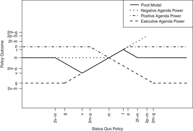
To ground what follows, Figure 1 plots equilibrium policy outcomes as a function of the location of the status quo relative to the ideal point of key actors for the pivot model and each agenda-setting model. Of course, the median voter model always produces an outcome at the median’s ideal point (m). In cases with no filibuster pivot, the pivot model predicts that policy will converge to the median’s ideal point (m) for all status quos on the opposite side of the median from the veto pivot (v).
Equilibrium policy outcomes. Note: This figure plots equilibrium outcomes for the pivot model and both party agenda-setting models. The policy preferences of the chamber median is denoted by m, the majority party median by p, the filibuster pivot by f, the veto pivot by v and the governor by g. The median voter model predicts a constant policy outcome of m.
The predictions in Figure 1 result from stylised models emphasising the importance of different institutional characteristics and different elites. None of the models are true in the sense of being able to explain the totality of what we observe, but the usefulness of these models is arguably best answered by investigating their ability to explain variation in law-making outcomes. If we see patterns that are consistent with theoretical predictions, the models can improve our understanding by providing some deeper insights into the meaning of the observed empirical correlations. In the absence of theoretical guidance, it can be difficult, if not impossible, to interpret the meaning of an empirical relationship. For example, a correlation between the preferences of the chamber median and policy outcomes could indicate at least three things: that the enacted policy outcomes exactly match the preferences of the chamber median voter as the median voter theory predicts, that the majority party median is proposing (and passing) policies strategically that make the chamber median at least indifferent to the status quo so that changes in the chamber median will change what the majority party is able to do, or that the chamber median is proposing policies to overcome the potential constraints imposed by the preferences of the governor or other veto-players in the law-making process.
Law-making theories can provide important leverage for interpreting the meaning of estimated relationships between policy outcomes and law-making participants, but determining whether actual law-making matches the predictions of the dominant spatial law-making models is difficult. One difficulty is that absent an ability to measure elite preferences and policy outcomes on the same scale, it is unclear how to relate observable law-making outcomes to theoretical predictions (Clinton Reference Clinton2017). Locating the policy preferences of the governor relative to the preferences of those legislators who would need to overcome a gubernatorial veto is difficult (see e.g. Treier Reference Treier2010 on the analogous difficulty in locating the president), as is locating the status quo and policy proposals in a way that can be directly compared with the measures of elite preferences (but see Peress Reference Peress2013).
Bridging theory and empirics with simulations
These measurement difficulties have secondary implications for how best to investigate the empirical support for the theoretical predictions graphed in Figure 1. One approach is to take a structural approach and to derive a likelihood function directly from the theoretical model (see e.g. Reiss and Wolak Reference Reiss and Wolak2007). Doing so requires an ability to measure all parameters of theoretical interest − in this case the preferences of all of the relevant actors, pivots, including the executive, as well as the location of the status quo − measures that are exceptionally elusive. A second approach is to adopt a reduced-form regression approach that identifies theoretically relevant covariates that are used to predict law-making activities and interpreting correlations between law-making outcomes and included covariates in terms of the predictions of competing law-making models.
Given the measurement difficulties involved in structurally estimating the theoretically implied relationships, we adopt a reduced-form approach. Even so, difficulties emerge − it is not obvious how to translate equilibrium predictions regarding policy outcomes into expectations about regression coefficients and it is not clear that a regression-based analysis of policy outcomes can adequately discriminate between the various models. Figure 1, for example, reveals that the equilibrium outcome for many of these models is a function of the chamber median’s ideal point m. Given this, absent an ability to measure policy and preferences on the same scale, how should we interpret a correlation between the chamber median and policy outcomes in terms of these four law-making models? Moreover, even if we find that conservative chamber medians are associated with more conservative policy, it is unclear what this correlation reveals about the relative support for the various theories because the location of the chamber median is important for every law-making model. Another difficulty is that because measures that are commonly used to characterise the policy preferences of relevant elites are highly correlated overtime (Wiseman and Wright Reference Wiseman and Wright2008) − legislatures with more conservative chamber medians are also more likely to have more conservative party medians − it can be hard to precisely estimate quantities of theoretical interest in a regression model.
Rather than assuming that correlations between measures of elite ideal points and policy outcomes are resolute for determining the model of lawmaking that is most likely responsible for the pattern of observed policies, we use a simulation study to characterise the pattern of partial correlations between the chamber median, majority party median, party of the governor and policy outcomes that are true for each law-making model. A simulation study provides us with predictions about the pattern of regression coefficients we should observe in a reduced-form regression if each theory were responsible for generating the data. By comparing these predictions with the pattern that we observe when applying the same regression specification to the data generated by state legislatures, we can identify the law-making theory that produces the most similar pattern of estimates. A simulation study is important because it reveals whether a simplified reduced-form specification containing only a few covariates can differentiate between competing law-making predictions, or whether more complicated statistical models are required.
We focus on the empirical relationship between policy outcomes and the ideal points of three political elites: the chamber median is important because of its importance in majoritarian systems (see e.g. Black Reference Black1958; Krehbiel Reference Krehbiel1998); the governor is important because they are sometimes empowered with a veto that requires a supermajority to override (Krehbiel Reference Krehbiel1998; Cameron Reference Cameron2000) and they may be able to mobilise public support (Canes-Wrone Reference Canes-Wrone2006; Kernell Reference Kernell2007); and the majority party median is of interest for determining whether the majority party is able to achieve its desired outcome in an electoral arena where voters may have little connection to their particular legislator beyond the party label (Cox and McCubbins Reference Cox and McCubbins2005).
To measure the policy preferences of these elites, we use the state legislative ideal points from 1993 to 2013 produced by Shor and McCarty (Reference Shor and McCarty2014).Footnote 2 Measuring the preferences of governors is more difficult, and we follow the existing literature in using the party of the governor as a proxy for policy preferences.Footnote 3 Although we focus on the composition of the lower house when conducting analyses in the text, including the composition of the upper chamber produces substantively identical results (see third section in the Online Appendix).
To collect information on cloture requirements − if they exist − we use a legislative research report based on data collected by the National Conference of State Legislatures to identify which chambers allow filibusters, and the votes that are required to overcome them (Reilly Reference Reilly2009). To allow filibusters, chamber rules must have no time limit on debate per legislator or in total and must require a supermajority to limit debate either through a motion to limit debate or move the previous question. We use the chamber rules that are most restrictive for each state (e.g. if the house does not allow filibusters but the senate does, we use the senate rules for that state).Footnote 4
Given these data and these rules, for each state and each time period we calculate the veto pivot and filibuster pivot according to the rules in each state. When computing the predictions of the pivot model, we set the veto pivot on the same side of the chamber median as the governor as defined by the proportion required to overcome a veto in the state (thereby assuming that the governor is at least as extreme as the veto pivot), and we identify the location of the filibuster pivot − if it exists − according to the proportion of votes required to end debate in the most restrictive chamber on the opposite side of the chamber median from the governor.Footnote 5
To perform the simulations and generate data that share the same properties as the data we use in later sections, we:
1. Draw an initial status quo for each of the 49 legislatures from a [−3,3] uniform distribution whose support coincides with the support of the distribution of estimated ideal points.Footnote 6
2. For each of the 49 legislatures:
a For each of the nine law-making periods:
Generate ideal points for each party using a Normal distribution characterised by the mean and standard deviation of ideal points of each party using the Shor-McCarty (Reference Shor and McCarty2014) estimates for the same chamber period. The size of each party in each legislature in each period is determined by the actual size of each party in the same chamber period (normalised to 100 legislators).Footnote 7 In each chamber period, the chamber median, majority party median and the filibuster and veto pivots are identified from the distribution of simulated legislators. We use the party of the governor to determine the correct side of the median for each pivot.Footnote 8
(a.1) For each of the four law-making models:
*Derive the equilibrium policy outcomes given the elite preferences from step 2a using the rules particular to each state and the location of the status quo inherited from the equilibrium outcome of the prior period (with the first period being generated in step 1).
3. Regress each set of policy outcomes on the chamber median, majority party median, party of the governor and a time trend along with state fixed effects using the same regression specification that we apply to the observed data. This includes both a level model (in the text) and a first-difference model (in the Online Appendix).
We replicate the steps outlined above to conduct 10,000 simulations that each produces a 49×9 matrix (49 states×9 time periods) of equilibrium outcomes for each of the five law-making models, as well as the matrix of generated ideal points used to generate the predictions. (The generated ideal points vary across the 10,000 simulations, but they are fixed across law-making models within each simulation.) Thus, each of the 10,000 simulations produces a data set that mirrors our observed data, but with policy outcomes that are produced by known models of lawmaking calculated using models that account for both the institutional variation across states and also the variation in ideal points overtime in each state.
To determine how the equilibrium predictions summarised in Figure 1 generate testable predictions in a reduced-form regression, we estimate the following specification for each of the 10,000 simulations:
 $$Y_{{i,t}} \, \, {\equals}\, \, \beta _{M} \,M_{{i,t}} {\plus}\beta _{P} \,P_{{i,t}} {\plus}\beta _{G} \,G_{{i,t}} {\plus}\tau \,{\rm time}{\plus}\gamma _{i} {\plus}{\epsilon}_{{i,t}} $$
where Y i,t is the equilibrium outcome for state i at time period t for a chosen law-making model, M i,t the ideal point of the (lower house) chamber median in state i at time t, P i,t the ideal point of the median member of the majority party in the lower house in state i at time t, G i,t an indicator for the presence of a Republican governor, τ the impact of a linear time trend to account for changing national conditions (e.g. federal grants for charter schools) and γ i a fixed effect for state i that accounts for persistent between-state differences (e.g. strength of teachers’ unions). Because the goal is to use the simulations to identify how the theoretical predications relate to the pattern of observed data and to explore our ability to distinguish between the theories using such a reduced-form specification, the specification we use is identical to the specification we use to analyse the actual pattern of law-making outcomes in later sections, the exception being that we use the equilibrium predictions of the various law-making models as Y i,t rather than measures of actual law-making outcomes.
Table 1 describes the resulting relationships. For each model, Table 1 reports the proportion of times a coefficient is positive and distinguishable from 0 using the simulated data. For example, the top row of Table 1 gives the proportion of the coefficients that are positive and distinguishable from 0 from the 10,000 regressions of the vector of 49×9=441 policy outcomes generated using the pivot model with a filibuster (if applicable) on the chamber median’s ideal point, the majority party median’s ideal point, an indicator for the governor’s party, state fixed effects, and a time trend. The coefficient on the chamber median’s ideal point is positive and distinguishable from 0 in every regression (100%), the coefficient on the majority party median’s ideal point is positive and distinguishable from 0 in fewer than half of the regressions (38%), and the indicator for a Republican governor is positive and distinguishable from 0 in every regression (100%). In contrast, when we use the same regression to analyse the set of policy outcomes produced by the median voter model, we find the chamber median covaries with the policy outcome in 100% of the regressions, but the ideal point of the majority party median is never positive and distinguishable from 0 and the party of the governor is also almost never positive and distinguishable from 0 (only 11% of the simulations).
Statistically significant correlations from simulation study.
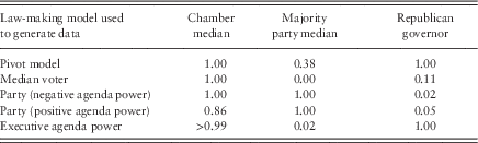
Note: Cell entries are the proportion of 10,000 ordinary least squares regressions of policy outcomes on elite preferences using legislative histories of length nine that produce correlation coefficients that are correctly signed and distinguishable from 0 with 95% confidence. Cell entries are rounded to two decimal digits. Regressions include state fixed effects and a time trend.
Several useful conclusions emerge from the simulation study. First, it is immediately clear that a single regression correlation coefficient cannot identify the theory responsible for generating the data. A positive association between the ideal point of the chamber median and policy outcomes, for example, is consistent with all five of the law-making models. Similarly, the regression coefficient for the ideal point of the majority party median is positively correlated with policy outcomes for every law-making model except the median voter model, although there is a positive and statistically significant correlation less often for the pivot model than for the party models. As a consequence, absent the simulation study, we would be unable to easily infer which law-making model is most consistent with regression models based on any single coefficient.
Second, the pattern of statistically significant coefficients is more resolute. Finding that only the coefficients on the chamber median and the Republican governor indicator are positive and statistically distinguishable from 0, for example, is most consistent with the pivot model or the executive agenda power model. The coefficient on party of the governor is positive and statistically significant in less than 11% of the simulations if the data are generated by the median voter model and less than 5% of the simulations if the data are generated by one of the party agenda power models. Alternatively, if only the ideal point of the chamber median is positively related to policy outcomes, the median voter model is most likely responsible for generating the data. If only the ideal points of the chamber median and majority party median are positive and significant (i.e. the indicator for the party of the governor is insignificant), then that pattern would be most consistent data generated by models of party agenda setting. Thus, the varying patterns of positive and statistically significant coefficients in Table 1 reveals that a simplified reduced-form model can be used to infer which law-making model is most consistent with the observed data. Moreover, the simulations are also useful for identifying when we cannot distinguish between theories using available data; finding a relationship with the chamber median and Republican governor, for example, is consistent with either a pivot-based theory in which the chamber median exercises agenda-setting power or else a situation where the executive wields agenda-setting power.
Third, the fact that the same regression specification produces different patterns of correlations depending on the law-making model used to generate the data justifies the use of this reduced-form specification for evaluating the competing law-making models. Even though we are not explicitly accounting for the ideal point of the governor, the simulation study results indicate that we do not need to do so to determine whether the pattern of law-making outcomes is more consistent with a pivot-based theory or a party-based theory so long as we include an indicator for the party of the governor. Thus, while we can imagine more elaborate empirical specifications, the simulation results suggest that the reduced-form specifications can distinguish between the law-making theories we examine.
To be clear, law-making models are a much-simplified version of reality that focus on certain aspects of lawmaking and omit others. Whether these simplifications are so severe so as to miss the primary determinants of lawmaking is an empirical question. If a model captures the primary law-making aspects, the pattern of statistically significant coefficients we observe when analysing simulated data resulting from that model should be observed in the patterns of actual lawmaking. If the models omit critical features of lawmaking at the state level, then the observed patterns may differ noticeably. Thus, while we may be concerned about the simplifying assumptions of each model, the utility of each model is ultimately determined by its ability to explain variation in lawmaking at the state level across the United States. Our simulation study suggests that a reduced-form empirical specification is sufficient for distinguishing between predictions, but we turn now to consider whether there is any evidence that the patterns of lawmaking we observe match these simulated patterns.Footnote 9
Measuring policy
The spatial law-making models of the prior section focus on the impact of various institutional rules on policy outcomes given two primitives: the policy preferences of elected officials and the location of the status quo policy. Progress has been made in characterising the ideal points of political elites (Poole and Rosenthal Reference Poole and Rosenthal1997; Clinton et al. Reference Clinton, Jackman and Rivers2004; Shor and McCarty Reference Shor and McCarty2011) – commonly assumed to describe policy preferences − but assessing policy change has proven more difficult. To make progress, we explore lawmaking in state legislatures (Hamm and Squire Reference Hamm and Squire2005; Squire Reference Squire2012) overtime using a general measure of the ideological content of policy, as well as policy measures related to the regulation of abortion and school choice in the states.
To measure the policy produced by the 49 state lower chambers over two decades, we use measures that vary in scope and content.Footnote 10 First, we use a measure of a state’s average policy liberalism that was produced by analysing the pattern of lawmaking across multiple issue areas overtime using a statistical measurement model (Caughey and Warshaw Reference Caughey and Warshaw2015b). Focussing on the dynamics of average state policy liberalism is important for providing an overall characterisation of state policy outcomes, but it can be difficult to detect subtle policy movements using a model-based average because of the limited impact that a single policy change can have on the average. Policy averages will measure concurrent unidirectional changes of multiple policies across time, but are not able to precisely measure changes in a single policy or cases where multiple policies change in conflicting directions (i.e. some policies become more conservative, whereas others become more liberal).
To explore the dynamics of particular policies, we therefore also analyse lawmaking on two salient policies with different relationships to national partisan divisions − the regulation of abortion and the establishment of charter schools.Footnote 11 Policy regulating the availability of abortion in a state is a highly salient and partisan issue on which state-level innovation is possible because of gridlock at the national level. It is also a well-defined issue with organised interests that are active nationally and clear ideological and party positions. Policies related to the establishment of charter schools provide an important and appropriate contrast. While charter school policy is also a salient issue that is largely, but not wholly, at the discretion of state legislatures, its connection to political ideology and parties is less well-defined (see the discussion in third section). The first charter school law was passed in Minnesota in 1991 and, between then and 2014, 42 states and the District of Columbia have adopted legislation allowing charter schools (for a total of 43 states that allow charter schools). Analysis of these two policies allows us to look at a mature policy with longstanding partisan positions (abortion) and a new policy that many states were debating and adopting for the first time during the period for which we have data (charter schools).
To characterise the content of, and change in, a state’s abortion policy overtime, we use the scorecard produced by NARAL Pro-Choice America. These ratings measure the cumulative burden of accessing reproductive health care in each state starting in 2004, and every state is scored every year on a 13-point grade scale ranging from F to A+.Footnote 12
These letter grades are presumably cardinal in the same way that letter grades in secondary schools are cardinal because they are based on an underlying numerical score − for example, the difference in policies between a state getting an A or a B is four times smaller than the policy differences between a state getting a B versus an F − but treating the scores as ordinal does not affect our findings. To measure the content of, and change in, a state’s laws related to the regulation of charter schools, we use the scores produced by the Center for Education Reform (CER), a pro-charter school interest group. These scores begin in 1997 and we scale them to range continuously from 0 to 1, with 0 indicating that charter schools are not allowed and 1 indicating that charter schools are allowed and have significant autonomy.Footnote 13
Interest group scores provide an appropriate and valuable measure of policy outcomes because they provide a summary score for each state in each year using standardised grading criteria. By using interest group scores, we avoid the difficult task of measuring policy using observable outcomes whose relationship to policy choices may be difficult to know and compare − for example, which of the multitude of educational outcomes related to “education policy” (i.e. dropout rates, standardised test scores) should be used to differentiate state policy and how is it possible to disentangle whether differences are due to state policy decisions or confounding considerations (e.g. parent involvement)? Interest groups’ desire to promote a particular policy outcome (e.g. more access to abortion, more autonomous charter schools) will not bias our analysis because we use the measure to characterise relative variation between states overtime − even if the rating system is systematically biased to favour a particular policy outcome this will not affect our ability to evaluate relative change because the scoring criteria are stable. Nor is it a problem that the policy scores may be influenced by actions of the judiciary or bureaucracy – actions taken by nonlegislative actors will only make it more difficult for us to find a relationship between the policy scores and the preferences of legislators. The actions of nonlegislative actors are also conceptually relevant because we are interested in the extent to which the policy change occurs relative to the status quo, not the last policy enacted by the legislature (which may no longer be policy relevant); legislators may enact a law to respond to judicial or bureaucratic action that alters the status quo.
Exploring the effect of some notable instances of policy change reveals the ratings’ sensibility. Between 2009 and 2012, Arizona enacted legislation that banned partial-birth abortions except to save the life of the mother, required notarised parental consent for a minor to get an abortion and banned abortions after 20 weeks of pregnancy (Rau Reference Rau2013; Florsheim Reference Florsheim2014). This sequence of policymaking resulted in their NARAL score declining from C+ in 2008 to D in 2009 to F in 2012. This change in policy coincides with the governorship changing party control from a Democrat to a Republican in 2009 and the election of increasingly conservative chamber and majority party medians. New Hampshire’s law authorising charter schools, for example, was first passed in 1995 and it was amended in 2003 to allow the State Board of Education to authorise charter schools (State of New Hampshire Charter School Program Review 2007). Because the CER considers the number of chartering authorities in their scoring, and laws that permit more chartering authorities receiving a higher (i.e. more conservative) score, this change in policy increased New Hampshire’s score by 3.5 points, or 10% of our 0–1 scale. This conservative change in policy coincided with the election of a Republican governor and more conservative chamber and majority party medians.
To provide a sense of the variation that exists in our overtime state-level policy measures, Figure 2 graphs the score of every state in the first period for which we have data [1992 for the policy liberalism score of Caughey and Warshaw (Reference Caughey and Warshaw2015b); 1997 for charter school policy; 2004 for abortion policy] against the state’s score as of 2014. Every scatter plot shows considerable between-state variation throughout the time period regardless of the measure being used. There is clear evidence that aggregate policy (i.e. state policy liberalism) and the particular policies of abortion and charter schools vary by state. Conversely, the within-state difference between the first and last observation of the aggregate measure is qualitatively different from the differences evident in the interest group measures even though the aggregate measure covers a longer time period. Because it is a model-based estimate of the state’s average policy in a latent dimension, the policy liberalism score changes only slightly between 1992–1994 and 2012–2014 within a state. In contrast, because the interest group scores focus on a single policy, the differences evident in the bottom graphs of Figure 2 reveal substantial overtime variation within states.Footnote 14
Net change in policy scores. Note: Higher values indicate more conservative policy positions. The 45° line denotes instances of no change.
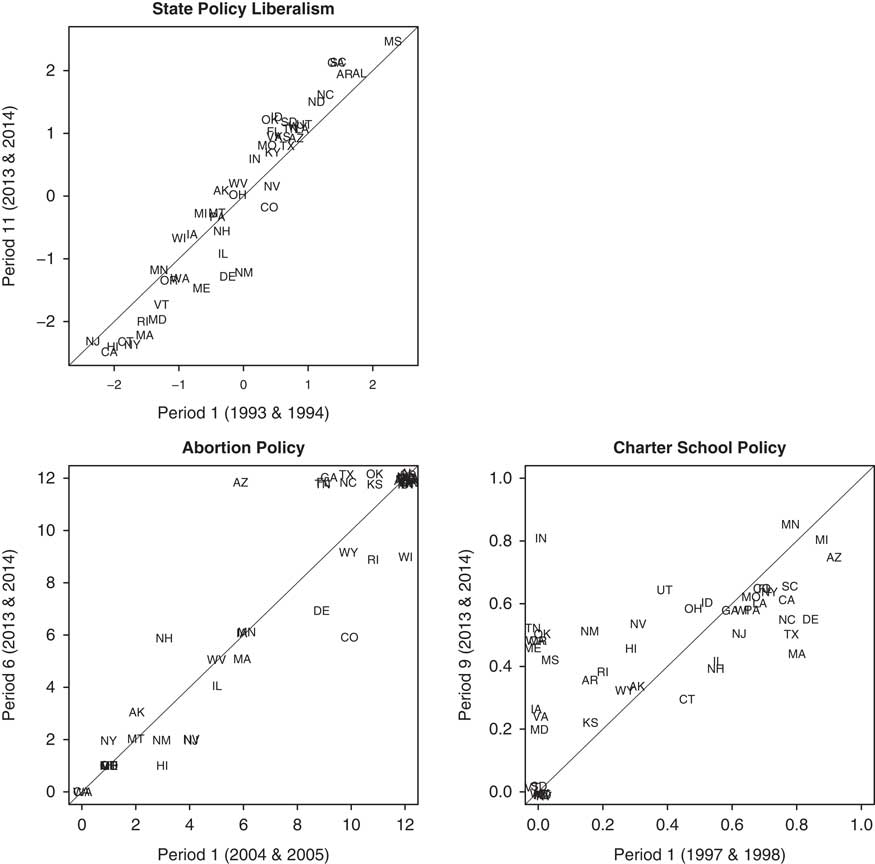
The lower right plot clearly reveals variation in the magnitude of change in states’ charter school policies. Importantly, the observed variation can be easily related to variation in the newly enacted policies. Among those states with no charter schools as of 1997 (i.e. a score of 0), the law enacted by Indiana in 2003 (0.79) − subsequently amended by legislative action to 0.82 as of 2013–2014 — allowed an unlimited number of charter schools to be sponsored by local school boards, five per year by public universities, and five per year by the mayor of Indianapolis, provided an automatic waiver from most state and district regulation, and gave charter schools full legal and fiscal autonomy. In contrast, the initial law enacted by Maryland in 2003 (0.24) was much more restrictive. It gave school districts the authority to determine the number of charter schools in each district, and while it allowed charter schools to apply for a waiver from state and district regulations it granted them only limited fiscal autonomy and no legal autonomy. Among states with preexisting charter school laws (i.e. states with scores greater than 0 as of 1997), some states chose to enact more permissive laws (e.g. Minnesota), whereas others placed more restrictions on charter schools (e.g. Kansas). Seven states did not enact a single pro-charter school law during the time period [the point mass at (0,0)].
Examining the net change in abortion policy (lower left plot) reveals several states that are graded as very conservative in both 2004 and 2014 [the point mass at (12,12)], but also that many states have notably altered abortion policy. While abortion regulations became more conservative in several states − the collection of points that are at 12 in period 6, but not period 1 − they also become more liberal in several others (those points beneath the 45° line).
Empirical results
We characterise the empirical relationship between the law-making outcomes described in second section and elites’ ideal points in two ways. First, we characterise the level of policy overtime and across states by modelling the policy score for each state in each time period controlling for differences in political elites’ preferences along with possible state and temporal differences. This specification exactly mirrors our simulation study by examining whether policy is more conservative in states where political elites are more conservative. Second, because policy is largely persistent overtime, we also explore how changes in policy relate to changes in elites’ ideal points. Doing so not only better accounts for the impact of policy persistence, but it also explores the speed of policy change − specifically, whether policy change occurs in the 2 years following each election.Footnote 15
To estimate the relationship between the conservatism of policy and elite ideal points across states i=1, … , 49 and time periods t=1, … , p, let Y i,t be either the policy liberalism score of Caughey and Warshaw (Reference Caughey and Warshaw2015b) or the policy score assigned to state i by the interest group as close as possible to the end of time period t.Footnote 16 We estimate the following specification:
 $$Y_{{i,t}} \, \, {\equals}\, \, \beta _{M} \,M_{{i,t}} {\plus}\beta _{P} \,P_{{i,t}} {\plus}\beta _{G} \,G_{{i,t}} {\plus}\tau \,{\rm time}{\plus}\gamma _{i} {\plus}{\epsilon}_{{i,t}} $$
where the constituent terms are as defined in first section. By allowing for systematic differences across states via the inclusion of γ i , we isolate the extent to which elite ideal points covary with a state’s policy score within states overtime. This is important because interpreting the meaning of cross-sectional variation is far more difficult given the many state characteristics that may affect policy outcomes − for example, whether the legislature is professional (Squire Reference Squire2007), the political strength of education reformers and teachers’ unions (e.g. Moe Reference Moe2006; Anzia Reference Anzia2011) and characteristics of the state’s educational system (e.g. Mintrom and Vergari Reference Mintrom and Vergari1998; Shober et al. Reference Shober, Manna and Witte2006). In contrast, a fixed effect estimator like the one we use controls for the impact of stable (i.e. time-invariant) state characteristics; for our estimates to be affected by omitted variable bias, the omitted variable must affect policy outcomes independent of elite preferences and vary within states across time in ways that are uncorrelated with the included time trend. (For robustness, fifth section of the Online Appendix shows that controlling for various state-level education characteristics produces nearly identical results.)
To measure the ideal points of the chamber and majority party medians, we use the composition of the lower chamber. Focussing on the lower chamber is conceptually sensible because the composition of the lower chamber is more likely to reflect the current political environment than the composition of the upper chamber because of more frequent elections, but replicating the results using the upper chamber does not change the results (see the Online Appendix). While it is possible to also include detailed measures of the veto pivot and filibuster pivot if appropriate given the rules particular to each state − not all states have rules requiring a supermajority vote to invoke cloture or override a veto − the simulation study in first section demonstrates that the pattern of regression coefficients from Equation (1) is sufficient for distinguishing between most law-making models.
To explore the possibility that the relationships depend on the level of legislative professionalisation in the state, we conduct all of the analyses separately for states with above and below average levels of legislative professionalisation using the measures of Bowen and Greene (Reference Bowen and Greene2014, Reference Bowen and Greene2016). Because we find substantively identical results, we focus on the pooled results to provide the most precisely estimated effects − the results by professionalism are reported in the Online Appendix.
Table 2 reports the results for the three outcome measures we examine: the policy liberalism (PL) measure of Caughey and Warshaw (Reference Caughey and Warshaw2015b), NARAL’s score for the state’s abortion policy (A) and CER’s score for the state’s charter school policy (CS). Newey-West standard errors are used to account for possible heteroskedasticity and autocorrelation. Including lagged policy scores produces qualitatively similar results (see Online Appendix).
Correlates of the level of policy
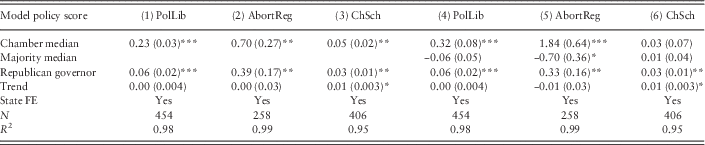
Note: Heteroskedasticity and autocorrelation consistent standard errors in parentheses.
FE=fixed effects.
*, **, ***Significant at p<0.10, p<0.05, p<0.01, respectively, in a two-sided test.
Several substantive conclusions emerge from Table 2. First, because policy is persistent within states across time and we include state fixed effects to account for between-state differences, the variation “explained” by the specifications is unsurprisingly high. That said, because the identification of the coefficients reported in Table 2 is based on within-state variation, the existence of non-zero partial correlations is strong evidence because the effect being detected is a consequence of variation occurring within states. Second, the results consistently suggest that Republican governors are, on average, more likely to enact more conservative policies than states with Democratic governors regardless of the ideal points of the chamber and majority party median.
Third, the results of Models 1, 2 and 3 reveal a robust relationship between the conservatism of the chamber median and policy conservatism when controlling for the party of the governor along with state fixed effects and a common time trend. Moreover, the relationship between the chamber median and policy outcomes increases in magnitude when including the ideal point of the majority party median and predicting overall policy liberalism (Model 4) and abortion policy (Model 5), but the relationship between the policy score and the majority party median is contrary to expectations. In terms of the implied substantive significance, a 1 SD conservative change in the ideal point of the chamber median is related to a 1.21 point change (0.66×1.84) in the 13-point policy score for abortion. The relationships between elite preferences and charter school policy outcomes are in the same direction across models; states with more conservative chamber medians adopt more conservative charter school policy (Model 3), but we can no longer distinguish this correlation from 0 when also controlling for the ideal point of the majority party median (Model 6).
The weaker relationships for charter school policy relative to abortion policy are likely attributable to how well the two policies map onto the partisan-cleavages captured by the ideal points of Shor-McCarty (Reference Shor and McCarty2014). Whereas the politics of abortion were consistently partisan and ideological across the time period we examine, the debate over charter schools was less clearly so. As of 1997, for example, California had a relatively permissive (i.e. “conservative”) charter school score of 0.78 despite having consistently liberal elites, whereas Wyoming only had a charter school law score of 0.27 despite having consistently more conservative elites. Between 1997 and 2014, however, California’s charter school law became more liberal (ending at 0.62) and Wyoming’s law became more conservative (ending at 0.32), but as of 2014 Wyoming’s policy on charter schools was still more restrictive (i.e. “liberal”) than California. In contrast, the initial scores for the abortion regulations in California and Wyoming were A+ (“liberal”) and D+ (“conservative”), respectively, and their scores remained unchanged through 2014. This difference not only illustrates why there is a stronger relationship in abortion policy than charter school policy in Table 2, but it also highlights the importance of moving beyond the analysis of levels of policy to also consider the correlates of policy change to account for the stability of policy across time.
To interpret the results in terms of extant law-making models, we compare the patterns of positive and statistically significant regression coefficients in Table 2 with the patterns from simulation study results reported in Table 1. The pattern of coefficients we find in Table 2 − positive and significant coefficients on the chamber median and Republican governor, but an insignificant coefficient on majority party median − was most frequently produced by data generated from simulations using either the pivot model or executive agenda-setting models of lawmaking. Whereas the majority party median was correlated with policy in 38% of the simulations using data generated from the pivot model, because we only have a single realisation of data and we are trying to infer the data-generating process it can be hard to conclusively interpret this aspect of the prediction. In contrast, it is highly unlikely that the median voter model could account for the pattern given the persistent significance of the Republican governor indicator, and the lack of correlation with the ideal point of the majority party median is contrary to the predicted relationships for the negative and positive agenda-setting predictions.
Overall, even though the results cannot determine whether the executive branch is powerful because of its veto (pivot model) or its agenda-setting power (executive agenda-setting model), the results are resolute in terms of revealing that law-making outcomes depend critically on both the legislative and executive branches and that accounts of lawmaking need to account for both to explain law-making activity. Focussing exclusively on the politics of either the legislature or the executive is therefore unlikely to yield an adequate characterisation of lawmaking. Additionally, models designed to explain lawmaking at the federal level also appear useful for explaining lawmaking at the state level.
Correlates of policy change overtime
Having shown that the level of policy is most closely associated with the ideal point of the chamber median in ways that are most consistent with the predictions of the pivot model or executive agenda setter, we now consider whether changes in policy correlate with changes in the composition of elected officials’ preferences. This is important not only because the persistence of policy across time within states makes it difficult to precisely identify the correlates of policy outcomes, but also because we can better control for the effect of the status quo on lawmaking. To do so, we use a first-difference model predicting the change in policy conservatism according to NARAL and CER as a function of the change in the ideal points of key legislators. We do not examine the change in the policy liberalism score of Caughey and Warshaw (Reference Caughey and Warshaw2015b) because Figure 2 reveals that there is almost no change over the time period we examine.Footnote 17
Our first-difference specification examines whether the policy change occurring between the election at time t and the election held at time t−1 correlates with the change in ideal points due to the election at time t−1. Put differently, does an election that results in elite turnover at time t−1 produce a change in policy as of time t that correlates with the estimated shift in ideal points? Note that if some legislatures wait longer (formally, until after the election at time t) to change policy, the first-difference model will underestimate the relationship. For example, suppose a majority party takes power at time t and it is reelected to the majority at time t+1 and it waits until time t+1 to change policy (perhaps because other issues are more pressing), the policy change between t−1 and t would be 0 even though elite preferences change between t−1 and t, and the policy change between t and t+1 would be non-zero even through there is no change in elite preferences.
To denote the empirical specification we use, let M i,t and P i,t be the ideal points of the chamber and majority party medians in state i at time t, respectively, and let G i,t indicate whether the governor is a Republican. Our basic estimating equation is as follows:
 $$(Y_{{i,t}} {\minus}Y_{{i,t{\minus}1}} )\, {\equals}\, \beta _{M} (M_{{i,t}} {\minus}M_{{i,t{\minus}1}} ){\plus}\beta _{P} (P_{{i,t}} {\minus}P_{{i,t{\minus}1}} ){\plus}\beta _{G} \,G_{{i,t}} {\plus}\gamma _{i} {\plus}{\epsilon}_{{i,t}} $$
where γ t is a fixed effect for state i. Because we continue to use state fixed effects to account for omitted between-state differences, the effect we estimate is due to within-state covariation. Because we include an indicator for a Republican indicator, β G measures whether policy drifts overtime depending on the partisanship of the governor; β G >0 implies that policy is drifting in a conservative direction holding the change in legislative ideal points constant. This could reflect the ability of the governor to influence policy through the administration and implementation of enacted legislation. The Online Appendix reports the results of applying this specification to the simulations studies described in first section and shows that this specification is able to distinguish between the theoretical predictions.
Table 3 reports the results from applying specification (2) to the observed law-making patterns involving changes in policies related to the regulation of abortion and charter schools. As the Online Appendix shows, allowing the relationship to vary by the level of legislative professionalism produces similar results, as does using the change in the governor’s party G i,t −G i,t−1 instead of a Republican indicator.
Correlates of policy change
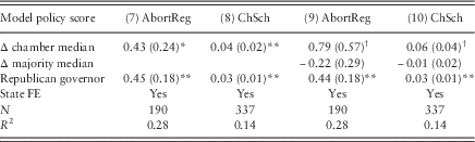
Note: Heteroskedasticity and autocorrelation consistent standard errors in parentheses.
FE=fixed effects.
*, **Significant at p<0.10, p<0.05, respectively, in a two-sided test.
†Significant at p<0.10 in a one-sided test of H A : β>0.
The findings in Table 3 are reassuringly consistent with the results of the level model in terms of the estimated relationships. First, the presence of a Republican governor is associated with more conservative policy changes on average. Whether this is because of the executive’s influence in law-making activities or because of the governor’s control over the bureaucracy responsible for implementing the policy change is unclear, but it is clear that the executive is important for policy changes in the states. To put the magnitude of the estimated relationships in perspective, the SD of the observed policy change is 0.82 for abortion regulations and 0.11 for charter school policies. As the Online Appendix shows, changes in the party controlling the governorship are correlated with changes in policy outcomes.
Second, controlling for the party of the governor, a conservative change in the chamber median is associated with a conservative change in policy for both abortion regulations (Model 7) and charter schools (Model 8). The fact that the chamber median is related to both the level and the change in policy outcomes is reassuring because it implies that not only is the chamber median closely connected to the level of policy enacted, but also that amendments to the existing policy are also likely related to changes in the chamber median.
Third, while the precision of these estimates slightly decreases after controlling for changes in the ideal point of the majority median, the relationship between changes in policy and changes in the ideal point of the chamber median persists (Models 9 and 10). Finally, as was the case in the level models reported in Table 2, there is no relationship between changes in the ideal point of the majority party median and changes in policy.
Comparing this pattern with the patterns produced by a simulation study investigating the expected predictions from estimating Equation (2) reveals that the patterns estimated in the observed data again best match the patterns produced by data generated from a data-generating process based either on the pivot model or the executive agenda-setting models of lawmaking (see Online Appendix).
The fact that changes in policy outcomes are correlated with changes in the ideal point of the chamber median is important because it reveals that the relationship between the chamber median and policy that was revealed in the level models of Table 2 is not simply a consequence of the fact that both are relatively stable overtime. There is a persistent relationship between the ideal point of the chamber median and the policy score within a state overtime and there is also a persistent relationship between changes in the ideal point of the chamber median and changes in the policy score within a state over time. This consistency suggests that our results are not simply attributable to chance and that the relationship is substantively meaningful. It also suggests, but certainly does not prove, that the pivot model emphasising the veto power of the governor may be a more reasonable explanation for the law-making patterns we observe because, all else equal, the equilibrium policy changes in a pivot model are smaller and less frequent that those in an executive agenda-setting model.
Conclusion and implications
Lawmaking is one of the most important actions that a legislature can take, but we know far more about how law-making works in theory than we do in practice. In part, this unfortunate gap is a consequence of the difficulty that scholars face when trying to characterise the magnitude of policy change overtime and across states in relation to changes in the composition of lawmakers. The gap is also likely related to the fact that we have largely assumed that explanations developed with the national government in mind apply equally to state governments despite the different electoral environments that state lawmakers face (Rogers Reference Rogers2016).
We use newly available data on the ideal points of political elites (Shor and McCarty Reference Shor and McCarty2014) and state policy (Caughey and Warshaw Reference Caughey and Warshaw2015b) along with policy scores provided by interest groups for two important and salient issues to provide a novel and revealing characterisation of state lawmaking over nearly two decades and across 49 legislatures. Our data allow us to examine the extent to which the preferences of political elites covary with the content and magnitude of policy change.
We find robust evidence of a substantively meaningful relationship between the ideal point of the chamber median and policy even when accounting for static systemic differences between states. Not only is the level of conservatism of the chamber median associated with the level of policy conservatism in a state, but the change in the conservatism of the chamber median is also associated with change in conservatism of state policy. We also find clear evidence that the partisanship of the governor also matters for both the level and change in policy. While our results do not identify the precise conditions under which governors are more or less influential – see, for example, Kousser and Phillips (Reference Kousser and Phillips2009) – and our results cannot determine whether governors’ influence is attributable to their veto or their ability to formally and informally set the agenda – the results unambiguously highlight the importance of the executive in determining the content of state policy.
Our finding that policy outcomes covary with the ideal point of the relatively “centrist” chamber median in terms of both the level and the change mirrors previous findings of Erikson et al. (Reference Erikson, Wright and McIver1993) and Battista et al. (Reference Battista and Richman2014). They are also consistent with a strong relationship that others have found between public opinion and state policymaking (Wright et al. Reference Wright, Erikson and McIver1987; Erikson et al. Reference Erikson, Wright and McIver1993; Lax and Phillips Reference Lax and Phillips2012; Caughey and Warshaw Reference Caughey and Warshaw2015a) given the connection between public opinion and the preferences of the median legislator. To be clear, because our results are based on the covariation of differently scaled measures, we cannot necessarily conclude anything about the proximity of policy outcomes vis-á-vis elite preferences and our results do not necessarily suggest that policy converges to the chamber median. Even so, our results suggest an influential role for the relatively centrist chamber median; not only do the policy scores vary with the ideal point of the chamber median within states, but the within-state changes in policy scores are also most closely associated with the changes in the chamber median’s ideal point.Footnote 18
Interpreting the meaning of these relationships in terms of law-making theories is possible because of the simulation study we conduct that relates law-making models to empirically predicted relationships. We are better able to identify what patterns of regression coefficients are and are not consistent with each of the law-making theories because we generate empirical predictions using simulations from data-generating processes that are known and determined by the law-making theories of interest. Doing so provides guidance for interpreting the patterns we estimate from the actual lawmaking by identifying the patterns predicted by each law-making theory in similar, but simulated, data.
The pattern we find in the observed data for both the level and first-difference models − positive correlations with the partisanship of the governor and the ideal point of the chamber median, but no systematic relationship with the ideal point of the majority party median − is most consistent with the patterns that result from a pivot model or an executive agenda-setting model. We cannot conclusively determine which model provides a better fit to the data given that both predict a similar pattern and it is certainly possible that both the informal agenda-setting powers of the governor due to their public position and the formal veto powers that they possess are responsible for their prominent impact on policymaking. Even when a governor appears to have limited formal authority − for example, governors in Tennessee can be overridden on a majority vote − our results suggest that they are nonetheless able to have an important impact on policymaking at the state level.
While these findings seem sensible − if not perhaps expected − it is important to emphasise that they are important in light of recent work questioning the extent to which understandings developed by studying the US Congress apply to state legislatures. Rogers (Reference Rogers2016), for example, shows that voters cast votes for state legislators based on what voters think about the party of the sitting US President and that the evidence for individual and collective accountability of state legislators is weaker than what others have found for the US Congress (Rogers Reference Rogers2017). While it may be consequently unclear how the seeming lack of electoral accountability for state legislators might affect the nature of lawmaking in state legislatures given the prominent connection between lawmaking and elections (e.g. Cox and McCubbins Reference Cox and McCubbins2005), our investigation reveals that lawmaking at the state and national level nonetheless appears to share common characteristics.
Acknowledgements
The authors would like to thank Steve Rogers and Alan Wiseman, as well as the reactions of anonymous reviewers during the review process, for helpful comments and reactions on earlier drafts.
Supplementary material
To view supplementary material for this article, please visit https://doi.org/10.1017/S0143814X17000265



