1 Introduction
Permeable porous materials are used extensively in various fields of engineering as filters and structural elements of cooling systems in devices with high thermal loads. There are some recent applications of gas-permeable porous materials for control of the aerodynamics of flying vehicles. At the moment, the area of application of permeable porous materials has been significantly extended. In particular, it is proposed to use gas-permeable porous materials for protection of various structures against shock waves (Ram & Sadot Reference Ram and Sadot2013), suppression of unsteady impingement of a supersonic jet onto a target (Zapryagaev et al. Reference Zapryagaev, Solotchin, Kavun and Yarovoy2011) and flow control in aerodynamics. Investigations aimed at using gas-permeable porous materials in aerodynamics are mainly performed in two directions:
(i) suppression of mean flow disturbances, namely, acoustic disturbances in a hypersonic boundary layer for extending the laminar flow regime (Fedorov et al. Reference Fedorov, Malmuth, Rasheed and Hornung2001, Reference Fedorov, Shiplyuk, Maslov, Burov and Malmuth2003; Maslov et al. Reference Maslov, Mironov, Poplavskaya, Tsyryulnikov and Kirilovskiy2012; Tsyryulnikov et al. Reference Tsyryulnikov, Maslov, Mironov, Poplavskaya and Kirilovskiy2015);
(ii) affecting the mean flow for the purpose of control of aerodynamic performance of flying vehicles.
The distinction between these aspects is rather conventional because the boundary layer flow regime exerts a considerable effect on the flow around the flying vehicle as a whole.
Within the framework of the second research direction, Nagamatsu, Orozco & Ling (Reference Nagamatsu, Orozco and Ling1984) and Bauer & Hernandez (Reference Bauer and Hernandez1988) showed that gas-permeable porous inserts in an aircraft wing in transonic flow eliminate flow separation induced by the closing shock wave. Hartman & Morgenstern (Reference Hartman and Morgenstern2004) in their patent propose to mitigate the intensity of the sonic boom generated by a supersonic aircraft with the use of gas-permeable porous inserts in the leading edges of the wing. In this case, porous materials ensure a required flow of air between the regions with an elevated static pressure on the shock wave, which decreases the intensity of the latter.
Hunter et al. (Reference Hunter, Viken, Wood and Bauer2001) proposed to use gas-permeable porous inserts for increasing the critical angle of attack by means of organizing air flow from the windward to the leeward side of the airframe. A gas-permeable porous insert ahead of a step on a flat plate in a supersonic flow allows one to control the separation region size (Fomin & Postnikov Reference Fomin and Postnikov2015). Bauer & Hemsch (Reference Bauer and Hemsch1994) attenuated vortex formation and reduced the side loads on a cylindrical body aligned at a non-zero angle of attack in a subsonic flow by using a gas-permeable porous nose cone. Fomin et al. (Reference Fomin, Zapryagaev, Lokotko and Volkov2009b , Reference Fomin, Zapryagaev, Lokotko, Volkov, Lutskii, Menshov, Maksimov and Kirdyashkin2010) experimentally demonstrated a method of drag reduction for a body in a supersonic flow by means of trapping some part of the incoming flow through the frontal gas-permeable insert and injecting it into the base region of the cylindrical model.
One of the methods of supersonic flow control is the use of a frontal gas-permeable porous insert. Fomin, Mironov & Serdyuk (Reference Fomin, Mironov and Serdyuk2009a
) demonstrated that the drag of a cylinder in a supersonic flow with
 $M_{\infty }=4.85$
can be significantly reduced by using an insert made of a high-porosity cellular material (HPCM) placed at the front face of the cylinder. The magnitude of the model drag can be controlled by increasing or decreasing the length of the porous insert protruding into the incoming flow. The physical pattern of the phenomenon implies the formation of an effective pointed body owing to the difference in the hydraulic resistance of the central and peripheral layers of the porous material of the frontal insert. An additional advantage of this method is the possibility of controlling the aerodynamic forces by means of local (Mironov, Maslov & Tsyryulnikov Reference Mironov, Maslov and Tsyryulnikov2014, Reference Mironov, Maslov and Tsyryulnikov2015b
) or global (Mironov, Poplavskaya & Kirilovskiy Reference Mironov, Poplavskaya and Kirilovskiy2017) heating of the frontal porous insert material without any mechanical displacements.
The degree of elaboration of the problem of using gas-permeable porous materials in supersonic aerodynamics is far from being sufficient because of the limited capabilities of experimental wind-tunnel and in-flight modelling; in particular, high Reynolds numbers and flow enthalpies corresponding to real flight conditions are not simulated in wind-tunnel tests.
The development of numerical methods ensures appreciable reduction of the time and expense needed for experimental investigations of complex flows and allows comprehensive parametric investigations of the process. Therefore, to develop engineering methods of design of supersonic flying vehicles with control surfaces containing gas-permeable porous inserts, it is necessary to have codes for computing the flow around various bodies with such structural elements. The use of such codes for parametric computations makes it possible to find the optimal structure of the porous material and the geometry of the porous insert. The basic element of the mathematical model, which is the basis of the numerical algorithm, is the model of a porous medium.
Continuum models with definition of the drag in the porous region in accordance with a certain law (e.g. Darcy filtration law, Darcy–Forchheimer law and others) are widely used to describe the flow in a porous medium. These comparatively simple models were developed as a result of mathematical treatment of empirical data obtained in studying filtration of fluids in soils under conditions of sufficiently low (within
 $10~\text{m}~\text{s}^{-1}$
) flow velocities and were later transferred to all types of motion of gases and liquids in porous media. For supersonic flows, the continuum approach with the use of the Darcy–Forchheimer law was applied for the first time in numerical simulations of the flow around a cylinder with a frontal cylindrical insert made of an HPCM by Bedarev et al. (Reference Bedarev, Mironov, Serdyuk, Fedorov and Fomin2011) and Mironov et al. (Reference Mironov, Maslov, Poplavskaya and Kirilovskiy2015a
). The results of those investigations revealed difficulties of using the continuum approach for modelling supersonic flows into high-porosity materials. The main problems were caused by drastic changes in the pressure gradient and filtration rate along the porous zone, which required derivation and application of different empirical laws of filtration along the porous insert.
The problem of high filtration rates in porous materials was solved numerically by Levy, Ben-Dor & Sorec (Reference Levy, Ben-Dor and Sorec1996) and Levi-Hevroni et al. (Reference Levi-Hevroni, Levy, Ben-Dor and Sorec2002, Reference Levi-Hevroni, Levy, Ben-Dor and Sorec2006) with the use of mass, momentum and energy conservation equations including terms associated with porous material characteristics (porosity, tortuosity and resistance). The influence of these parameters on gas filtration in porous samples at moderate Mach numbers was studied. However, this approach was not tested in problems of a supersonic flow around a body with a porous insert.
Another approach to solving the problem of a supersonic flow around a cylinder with a frontal porous insert is direct numerical simulation of the gas flow in the porous material skeleton. In this case, the porous material is characterized by the skeleton geometry and porosity, without using any empirical laws of filtration. This approach was successfully applied in Kirsanov, Nazipov & Danilov (Reference Kirsanov, Nazipov and Danilov2011) and Mitrichev, Koltsova & Zhensa (Reference Mitrichev, Koltsova and Zhensa2012) for obtaining data on the hydraulic resistance and heat transfer in the HPCM in a low-velocity gas flow. At high velocities of the flow, skeleton models of porous materials were successfully used in numerical simulations of suppression of acoustic disturbances in hypersonic boundary layers (Sandham & Ludeke Reference Sandham and Ludeke2009; Maslov et al. Reference Maslov, Mironov, Poplavskaya, Tsyryulnikov and Kirilovskiy2012; Wartemann, Ludeke & Sandham Reference Wartemann, Ludeke and Sandham2012; Tsyryulnikov et al. Reference Tsyryulnikov, Maslov, Mironov, Poplavskaya and Kirilovskiy2015). In numerical simulations of drag control problems for bodies with porous inserts, skeleton models were used for the first time by Mironov et al. (Reference Mironov, Poplavskaya and Kirilovskiy2017) and Kirilovskiy et al. (Reference Kirilovskiy, Maslov, Mironov and Poplavskaya2018). For an axisymmetric flow around a cylinder with a frontal high-porosity insert, a simple skeleton model of the porous medium was proposed: a system of coaxial rings of different diameters arranged in a staggered order in the radial and streamwise directions.
Application of this method in aerospace engineering requires extensive scientific investigations. First of all, this is needed for identification of physical mechanisms inherent in this method and also the influence of the basic flow parameters on these mechanisms. Moreover, one of the fundamental aspects of the problem of a supersonic flow around a body with a frontal porous insert is finding similarity criteria that allow one to determine the model drag in a supersonic flow for various flow conditions and scales of the model. Therefore, it is these fundamental aspects of the problem that are considered in the present paper.
To find the main features of the process and optimize the effect of HPCM inserts, experimental and numerical parametric investigations were performed in the present work to study a supersonic flow around a cylinder with a frontal insert made of cellular-porous nickel with porosity of 0.95 with variations of the HPCM cells, cylinder diameter, and Mach and Reynolds numbers. Based on the present simulations and experiments, a possibility of controlling the aerodynamic characteristics of bodies with gas-permeable HPCM inserts was demonstrated and the mechanisms of drag reduction in supersonic flows were described. An empirical dependence of the normalized drag coefficient on a parameter which includes the ratio of the cylinder diameter to the pore diameter in the insert and the Mach number was derived. This parameter can be considered as a similarity criterion for the problem of a supersonic flow around a cylinder with a frontal HPCM insert.
2 Experiment
The experiments for the flow around a cylinder with a frontal porous insert were performed in a T-327 supersonic blowdown wind tunnel based at the Khristianovich Institute of Theoretical and Applied Mechanics, Siberian Branch, Russian Academy of Sciences (ITAM SB RAS). The wind tunnel is a free-jet facility with the jet escaping into a vacuum tank. The run time is 40 s. The output diameter of the wind-tunnel nozzle is 0.22 m. The experiments at Mach number
 $M_{\infty }=4.85$
were performed at the stagnation pressure
 $p_{0}=0.5$
–10 atm and constant stagnation temperature equal to
 $T_{0}=295$
K. The experiments at
 $M_{\infty }=7$
were performed at the stagnation pressure
 $p_{0}=1$
atm and
 $T_{0}=295$
K. The experiments at
 $M_{\infty }=21$
were conducted at
 $p_{0}=80$
atm and
 $T_{0}=1200$
K. The upper limits of the stagnation pressure for each Mach number are caused by the necessity of avoiding test gas condensation (Daum & Gyarmathy Reference Daum and Gyarmathy1968). The experiments were performed in the range of unit Reynolds numbers
 $Re_{1\infty }=(0.7{-}13.5)\times 10^{6}~\text{m}^{-1}$
at
 $M_{\infty }=4.85$
,
 $Re_{1\infty }=1.5\times 10^{6}~\text{m}^{-1}$
at
 $M_{\infty }=7$
, and
 $Re_{1\infty }=0.6\times 10^{6}~\text{m}^{-1}$
at
 $M_{\infty }=21$
. The Reynolds number at
 $M_{\infty }=4.85$
was varied by changing the stagnation pressure in the settling chamber of the wind tunnel.
HPCM samples with the porosity
 $k=0.95$
(ratio of the volume of voids in the material to its total volume) and with the pore diameter
 $d=1$
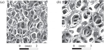
, 2, 3 and 4 mm were used. This material is the result of solidification of foamed liquid metals (nickel in the present case). The solidified metal foam forms a three-dimensional skeleton composed of partitions between neighbouring cells. This process allows production of high-porosity materials with porosity ranging from 0.76 to 0.98. If the porosity is lower, the material is not permeable for the gas; if the porosity is higher, no skeleton is formed. An enlarged image of a fragment of the cellular-porous nickel structure is shown in figure 1. Detailed parameters of this porous material can be found in Belov (Reference Belov and Belov1987).
Enlarged image of fragments of porous nickel inserts: (a)
 $d=1$
mm and (b)
 $d=3$
mm.

The model of the cylinder with the frontal gas-permeable HPCM insert is shown in figure 2(a). The model had the diameter
 $D=14.5$
, 24 and 34 mm; the porous insert length
 $\unicode[STIX]{x0394}x$
was varied from zero to
 $3.1D$
mm with the use of a moving thin-walled tube closely adjacent to the cylinder. The tube could be moved over the cylinder, covering the porous insert partially or completely. The total length of the model was 100, 120 and 140 mm for
 $D=14.5$
, 24 and 34 mm, respectively. The experimental model of the cylinder consisted of three parts: frontal porous insert, porous material covered by the moving thin-walled tube, and solid cylinder. Special experiments for the flow around such an experimental model consisting of three parts showed that the gas in the HPCM region covered by the thin-walled tube did not move at all; hence, this part of the model could be replaced by a solid cylinder. In that experiment, the drag forces generated by the model with a completely closed porous insert and by the model of a solid cylinder were measured and were found to be identical.
Experimental model of a cylinder (a) with a frontal gas-permeable insert with
 $d=1$
mm and (b) with an aerospike.

The drag forces of a cylinder with a diameter
 $D=14.8$
mm and a blunted aerospike 1.5 mm in diameter, which had a variable length, were additionally measured (see figure 2
b). The experiments with the aerospike were performed for the Mach number
 $M_{\infty }=4.85$
and Reynolds number
 $Re_{1\infty }=2.7\times 10^{6}~\text{m}^{-1}$
, and also for
 $M_{\infty }=7$
and
 $Re_{1\infty }=1.5\times 10^{6}~\text{m}^{-1}$
.
The model was mounted on a three-component strain-gauge balance, which measured the drag force generated by the model. The model was fixed on the balance by a long pin 2 mm in diameter, which was screwed into the centre of the rear end face of the solid cylinder. It should be noted that the error in the experimental data was determined on the basis of scattering of balance measurement results in a large number of experiments performed at different times. In addition, schlieren visualization of the flow around the model was performed.
3 Skeleton model of a gas-permeable porous medium
One of the main problems in designing the HPCM model skeleton is obtaining the mean characteristics of the flow with the minimum number of assumptions concerning the skeleton geometry. Therefore, the HPCM skeleton in the present work was designed under the following two assumptions.
(1) In an axisymmetric flow around the HPCM sample, gas inside the porous material basically moves in the streamwise and radial directions only, because the gas motion in the azimuthal direction is negligibly small owing to the random arrangement of pore partitions and the absence of the azimuthal pressure difference in the sample.
(2) The governing parameters of the model are the porosity, HPCM pore size and reference length of material transparency. This assumption was confirmed by Mitrichev et al. (Reference Mitrichev, Koltsova and Zhensa2012), where a three-dimensional structure of the HPCM skeleton shaped as an array of overlapping spheres was used. (Here the reference length of material transparency is the maximum thickness of the porous material through which direct transmission of light is possible. This characteristic means that the streamlines cannot directly reach the end face of the solid part of the model.)
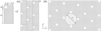
Numerical simulations were performed by using a porous medium model shaped as a system of staggered coaxial rings of different diameters (figure 3). In the plane of the axial cross-section, this system of rings (porous material skeleton) is a set of staggered impermeable elements (figure 4 b).
Three-dimensional image of the computational model: here
 $d=1$
mm.

This skeleton model has no radial partitions between the ring elements. As compared to HPCM skeleton models (e.g. tubular–spherical model of Kirsanov et al. (Reference Kirsanov, Nazipov and Danilov2011) or a system of hollow intersecting spheres of Mitrichev et al. (Reference Mitrichev, Koltsova and Zhensa2012), which have a rather complicated three-dimensional structure), the proposed skeleton model is fairly simple to design the porous region in the axisymmetric case.
Skeleton design begins from constructing a single rectangular domain (figure 4
a), which includes one cross-section of the ring element (
 $lx\times lr$
). The domain size is
 $(d+lx)/2$
in the axial direction and
 $d+lr$
in the radial direction. In each domain, the skeleton element area is 5 % of the total domain area, which corresponds to the HPCM porosity coefficient of 0.95. If this condition is satisfied, it is possible to determine the shape (square or rectangular) and size (
 $lx,lr$
) of skeleton elements. After that the entire area of the axial section of the porous insert is filled with such domains arranged in a staggered order (figure 4
b). In this case, it is possible to inscribe a circle of diameter
 $d$
equal to the pore diameter in a real HPCM sample into the space between four skeleton elements (see figure 4
b). The axisymmetric model of the skeleton is formed by means of rotating the square elements around the longitudinal axis of the model.
(a) Skeleton design principle and (b) projection of the HPCM skeleton model onto the
 $x$
–
 $r$
plane with the representation of the computational grid (here
 $d=1$
mm).

Additional characteristics of the HPCM are the random arrangement of the skeleton elements and the length of material transparency. Therefore, the vertical row of domains is gradually shifted in the computational model to ensure correspondence with the length of real HPCM transparency (see figure 4 b). This fact is illustrated in the image of the model porous insert in figure 3 as a periodically repeated step on the external boundary of the porous insert.
The HPCM skeleton design is given by an example of a material with a pore diameter of 1 mm. For materials with greater pore diameters, the general pattern of skeleton construction is the same, but the cross-sectional shape of the ring elements and the radial distance between these elements are changed to compensate for the absence of radial partitions of the model skeleton. For the material with
 $d>2$
mm, the skeleton model is a system of rectangular elements rotated around the axis of symmetry (coaxial ring structures with a rectangular cross-section). It should be noted that the HPCM skeleton design procedure is identical if the present simplified skeleton model is applied in three-dimensional simulations. The advantage of this skeleton model is the possibility of using a structured computational grid, in contrast to HPCM skeleton models with a complicated spatial structure, which require only unstructured grids to be used.
4 Numerical simulation
The axisymmetric flow around the cylinder with model inserts was numerically simulated by the commercial package ANSYS Fluent. The problem was solved within the framework of two-dimensional Reynolds-averaged Navier–Stokes (RANS) equations written in an axisymmetric form (see §§ 1.2 and 5.2.1.1 of the ANSYS Fluent 18.0 Theory Guide) in a cylindrical coordinate system
 $x$
–
 $r$
(
 $x$
and
 $r$
are the axial and radial coordinates). The system of equations is supplemented with the equation of state for a perfect gas and with the
 $k{-}\unicode[STIX]{x1D714}$
shear stress transport (SST) turbulence model (Menter Reference Menter1994) built in to the package (see § 4.4.3 of the ANSYS Fluent 18.0 Theory Guide). The turbulent flow regime was chosen because of the presence of jets exhausting from the porous material to the flow around the model and their eddying effect.
Within the framework of the software package, the problem of an axisymmetric flow around a cylinder was solved with the use of implicit schemes of second-order accuracy in space. Convective fluxes were approximated by the Roe flux difference splitting (FDS) method of splitting with a total variation diminishing (TVD) limiter for retaining solution monotonicity near discontinuities and local extreme points of the flow.
Projection of the computational domain onto the
 $x$
–
 $r$
plane with the representation of splitting into individual regions and grid refinement direction.

The projection of the computational domain onto a plane (figure 5) is a rectangle, and its lower boundary coincides with the axis of symmetry of the cylinder. The left (input) boundary is located at a distance of 50 computational cells upstream from the front face of the model, and the computational domain height was chosen under the condition that the bow shock wave (SW) did not interact with the upper boundary of the computational domain. The right (output) boundary was shifted from the rear face of the model to a distance of the order of the model length. The computational domain consisted of several subdomains (region ahead of the body, region of the porous insert, and region behind the porous insert) in order to provide grid refinement near the bow SW and the cylinder surface, and to minimize the number of cells in the computational domain. The porous subdomain was covered by a uniform rectangular computational grid with an integer number of computational cells on each side of the individual element of the HPCM skeleton (see figure 4). The total number of cells in the entire computational domain was varied from 200 000 to 1200 000 (the greater the porous region length or the cylinder diameter, the greater the total number of cells). The computational grid satisfies the condition
 $y+<1$
(or
 $y+$
approaches unity) on all surfaces (including those of the elements inside the porous region).
Grid refinement by a factor of 2 in both directions revealed that the flow characteristics (velocity, density, pressure and drag coefficient) changed by less than 2 %. To estimate the numerical errors, we also applied the grid convergence index (GCI) method (Roache Reference Roache1994) based on the Richardson extrapolation (Richardson Reference Richardson1927). The GCI value shows how closely the numerical solution approaches the exact asymptotic solution. The GCI for the fine grid solution is calculated by the formula:
 $$\begin{eqnarray}\text{GCI}_{i,i+1}=Fi\frac{e_{i,i+1}}{r^{q}-1},\quad e_{i,i+1}=\frac{|\,f_{i+1}-f_{i}|}{f_{i}}.\end{eqnarray}$$
Here
 $f$
is the solution on the
 $i$
th grid,
 $e_{i,i+1}$
is the normalized error between the
 $i$
th and (
 $i+1$
)th solutions (the subscript
 $i+1$
corresponds to a coarser grid),
 $Fi$
is the safety factor (here
 $Fi=1.25$
is based on experience applying GCI in many situations (Roache Reference Roache1994)), and
 $r$
is the grid refinement coefficient. After solving this problem on three gradually refined grids with an identical grid refinement coefficient
 $r$
, the local accuracy of the solution
 $q$
can be written in the following form (Richardson Reference Richardson1927):
 $$\begin{eqnarray}q=\frac{\ln ((f_{3}-f_{2})/(f_{2}-f_{1}))}{\ln (r)}.\end{eqnarray}$$
The exact solution
 $f_{exact}$
is estimated by the formula:
 $$\begin{eqnarray}f_{exact}=f_{1}+(f_{1}-f_{2})/(r^{q}-1).\end{eqnarray}$$
In the present work,
 $f$
is the drag coefficient of the cylinder with the porous insert,
 $C_{x}$
. The base variant (
 $M_{\infty }=4.85$
,
 $p_{\infty }=186$
Pa,
 $T_{\infty }=51$
K,
 $Re_{1\infty }=2.7\times 10^{6}~\text{m}^{-1}$
,
 $\unicode[STIX]{x0394}x/D=2$
and
 $d=1$
mm) was computed on three gradually refined grids: grid 3 with 201 000 cells, grid 2 with 454 000 cells, and grid 1 with 1029 000 cells. Thus, the grid refinement coefficient was
 $r=1.5$
, because the grid steps in both directions were reduced by a factor of 1.5. The drag coefficients of the cylinder with the porous insert,
 $C_{x}$
, obtained on grids 1, 2 and 3 are listed in table 1. The normalized errors between the solutions and the GCI values calculated by the above-mentioned gradually refined grids with an identical refinement coefficient
 $r=1.5$
are listed in table 2.
Drag coefficients of the cylinder with the porous insert for three gradually refined grids.

Parameters of GCI analysis.

Based on the data obtained on grids 2 and 1, the value of
 $\text{GCI}_{1,2}$
was equal to 0.04 %. The
 $\text{GCI}_{1,3}$
value for grid 3 was estimated as
 $\text{GCI}_{2,3}\times r^{q}$
(Roache Reference Roache1994) and was found to be 1.82 %. This means that the computational grid 3 (201 000 cells) is suitable for further computational fluid dynamics (CFD) analysis, and the numerical solution obtained on this computational grid differs from the exact asymptotic solution by less than 1.82 %.
Up to 10 processors of the Information-Computational Center of the Novosibirsk State University and the Siberian Supercomputer Center were used in the computations.
The problem was calculated by a time-dependent method. The left (input) boundary of the computational domain was subjected to the free-stream conditions
 $p_{\infty }$
,
 $M_{\infty }$
,
 $T_{\infty }$
and the laminar flow condition (
 $k=\unicode[STIX]{x1D714}=0$
) for the
 $k{-}\unicode[STIX]{x1D714}$
SST turbulence model. Flow exhaustion was imposed at the right (outflow) boundary, and the symmetry condition was set at the upper boundary. The cylinder surface and each element of the porous insert skeleton were subjected to the no-slip condition and a constant temperature
 $T_{w}=290$
K.
Solving the problem, we obtained all gas-dynamic variables of the flow both outside the model and inside the porous material. Based on these data, we determined the bow shock wave position, the shape of the effective (conventionally impermeable) body, the isolines of the density gradient, and the drag coefficient of the model,
 $C_{x}$
.
For comparison with the experiments, the present computations were performed on the basis of an integral method of drag calculations based on the momentum loss of the flow in order to take into account not only the drag due to the body shape, but also the drag induced by friction on the multi-element skeleton of the porous insert. The drag coefficient of the model was calculated as
 $C_{x}=F/(0.5\unicode[STIX]{x1D70C}_{\infty }u_{\infty }^{2}S_{m})$
, where
 $\unicode[STIX]{x1D70C}_{\infty }$
and
 $u_{\infty }$
are the free-stream density and velocity,
 $S_{m}$
is the cross-sectional area of the model, and
 $F$
is the aerodynamic force, which consists of the pressure force including the wave drag and the friction force. In this work, the force
 $F$
was calculated from the difference in the total momentum of the flow in two cross-sections: (1) ahead of the bow SW and (2) in the plane of the rear end face of the cylinder (integral over the area of the examined cross-section), i.e.
 $F=\int _{S_{1}}(p_{\infty }+\unicode[STIX]{x1D70C}_{\infty }u_{\infty }^{2})\,\text{d}s-\int _{S_{2}}(p_{2}+\unicode[STIX]{x1D70C}_{2}u_{2}^{2})\,\text{d}s$
. Here
 $S_{1}$
is the cross-sectional area of the computational domain at the input boundary and
 $S_{2}$
is the cross-sectional area of the computational domain at the streamwise coordinate corresponding to the position of the rear end face of the cylinder. Thus, we calculated the drag coefficients
 $C_{x}$
of the cylinder with the frontal porous insert and
 $C_{x0}$
of the solid cylinder.
5 Results
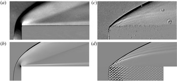
Figure 6 shows the schlieren pictures of the flow obtained in the experiments and the computed isolines of the density gradient in the normal direction to the
 $x$
axis in the flow around the solid cylinder and the cylinder with the frontal porous insert of length
 $\unicode[STIX]{x0394}x/D=1.93$
. It is seen that the experimental and predicted flow patterns are in good agreement. Figure 6 clearly shows the transition from the arc-shaped bow SW on the solid cylinder to the oblique shock in the presence of the gas-permeable porous insert. In the case with this length of the gas-permeable insert, the bow SW enters the porous material, giving rise to weaker oblique shocks induced by outflow of air filaments from the pores. The present studies demonstrate the transformation of the intense bow SW into a system of oblique shocks. This leads to significant attenuation of the bow SW and, as a consequence, to reduction of the SW stand-off distance from the surface of the porous insert.
Schlieren pictures of the flow obtained in the experiments (a,c) and computed isolines of the density gradient in the normal direction to the
 $x$
axis (b,d): (a,b) experiment and computation for a solid cylinder and (c,d) experiment and computation for
 $d=1$
mm. Here
 $D=14.5$
mm,
 $M_{\infty }=4.85$
,
 $p_{\infty }=186$
Pa,
 $T_{\infty }=51$
K,
 $Re_{1\infty }=2.7\times 10^{6}~\text{m}^{-1}$
and
 $\unicode[STIX]{x0394}x/D=1.93$
.

Comparison of experimental (1–3) and computed (4–7) positions of the bow SW: (1,4) solid cylinder; (2,5)
 $\unicode[STIX]{x0394}x/D=0.34$
,
 $d=1$
mm; (3,6,7)
 $\unicode[STIX]{x0394}x/D=2.0$
,
 $d=3$
mm; (4,5,6) skeleton model, (7) continuum model from Mironov et al. (Reference Mironov, Maslov, Poplavskaya and Kirilovskiy2015a
). Here
 $D=14.5$
mm,
 $M_{\infty }=4.85$
,
 $p_{\infty }=186$
Pa,
 $T_{\infty }=51$
K,
 $Re_{1\infty }=2.7\times 10^{6}~\text{m}^{-1}$
.

The experimental data (symbols) and numerical predictions (curves) for the shape of the bow SW on the solid cylinder and the cylinder with the frontal porous insert with different pore diameters are compared in figure 7. It is seen that an increase in the gas-permeable insert length changes the flow field around the cylinder: in the case of the solid cylinder, the bow SW moves away from the front face of the model. In the case of the cylinder with the frontal gas-permeable insert, the bow SW approaches the front face of the model; moreover, at
 $\unicode[STIX]{x0394}x/D=2$
, the bow SW becomes attached to the front plane of the cellular porous insert. It should also be noted that the SW slopes become almost identical at a sufficiently large distance from the front face of the porous insert. However, the main difference in the SW shape is observed in the region of the SW curvature near the front face. It is this region that is responsible for the greatest loss of the total momentum of the flow. However, the primary reason for such changes in the SW curvature near the front face of the cylinder is attenuation of the bow SW by weak oblique shock waves because of fluid exhaustion through the front and side pores of the material.
For
 $d=3$
mm, figure 7 also shows the SW position predicted by the continuum model by Mironov et al. (Reference Mironov, Maslov, Poplavskaya and Kirilovskiy2015a
). It is seen that the skeleton model of the porous insert provides a more accurate reproduction of the bow SW (it is more curved, like that in the experiment). The continuum model predicts a smaller slope of the bow shock wave. This difference in the SW position in space is caused by the fact that the leading edge of the porous insert is essentially non-uniform because of the presence of pores and finite-size partitions in both the experiment and computations by the skeleton model.
Figure 8 shows the streamlines for the cases of the flow around a solid cylinder and a cylinder with a frontal porous insert of length
 $2D$
(
 $\unicode[STIX]{x0394}x/D=2$
). It is seen that the angle of flow turning in the case with the porous insert is smaller than that in the case with the solid cylinder. Such gas flow redistribution in the cellular porous body leads to a flow similar to the flow around a pointed body, resulting in model drag reduction in the supersonic flow. Such a pointed solid body is conventionally considered as an impermeable body, and its drag coefficient is equal to the drag coefficient of the cylinder with the frontal porous insert.
Streamlines: (a) solid cylinder; (b) cylinder with a gas-permeable insert with
 $\unicode[STIX]{x0394}x/D=2$
. Here
 $M_{\infty }=4.85$
,
 $p_{\infty }=186$
Pa,
 $T_{\infty }=51$
K,
 $Re_{1\infty }=2.7\times 10^{6}~\text{m}^{-1}$
.

A conventionally impermeable body is a solid body whose drag is equal to the drag of a cylinder with a frontal porous insert. By definition, the shape of the effective (conventionally impermeable) body is characterized by the displacement thickness, which is found from the calculated velocity and density fields:
 $\unicode[STIX]{x1D6FF}^{\star }(x)=\int _{0}^{\infty }[1-\unicode[STIX]{x1D70C}u(x,y)/\unicode[STIX]{x1D70C}_{\infty }u_{\infty }]\,\text{d}y$
. The results calculated by this formula for the solid cylinder and for the cylinder with the frontal porous insert are shown in figure 9. It is seen that the conventionally impermeable body has a pointed shape in the case of the flow around the cylinder with the frontal gas-permeable insert.
Displacement thickness: (1) solid cylinder; (2) cylinder with a gas-permeable insert with
 $\unicode[STIX]{x0394}x/D=2$
,
 $D=14.5$
mm,
 $d=1$
mm. Here
 $M_{\infty }=4.85$
,
 $p_{\infty }=186$
Pa,
 $T_{\infty }=51$
K,
 $Re_{1\infty }=2.7\times 10^{6}~\text{m}^{-1}$
.

The experimental and computed normalized drag coefficients of the model,
 $C_{x}/C_{x0}$
, are plotted in figure 10 as functions of the normalized length of the porous insert
 $\unicode[STIX]{x0394}x/D$
. Normalization is performed to the drag coefficient
 $C_{x0}$
of the cylinder without the porous insert, which is given in table 3 for
 $M_{\infty }=4.85$
.
Experimental (1,2,3,4,8,9) and computed (5,6,7) data for the normalized drag coefficient of the model versus the normalized length of the porous insert: (1,5)
 $d=1$
mm; (2)
 $d=2$
mm; (3,6,7)
 $d=3$
mm; (4)
 $d=4$
mm; (7) continuum model from Mironov et al. (Reference Mironov, Maslov, Poplavskaya and Kirilovskiy2015a
); (5,6) skeleton model, with
 $D=14.5$
mm,
 $M_{\infty }=4.85$
,
 $p_{\infty }=186$
Pa,
 $T_{\infty }=51$
K,
 $Re_{1\infty }=2.7\times 10^{6}~\text{m}^{-1}$
, HPCM
 $k=0.95$
; (8) mesh layers,
 $k=0.7$
; (9) metallic felt cloth,
 $k=0.25$
.

Drag coefficient of the cylinder without the porous insert, with
 $D=14.5$
mm,
 $L=100$
mm.

Figure 10 shows the experimental data for different pore diameters
 $d=1$
and 3 mm (Fomin et al.
Reference Fomin, Zapryagaev, Lokotko and Volkov2009b
) and
 $d=2$
and 4 mm (present work). The results of computations based on the skeleton model of a porous medium are shown in figure 10 by the dashed curves. The solid curve illustrates the results for the flow computed by the two-zone continuum model for the pore diameter
 $d=3$
mm (Mironov et al.
Reference Mironov, Maslov, Poplavskaya and Kirilovskiy2015a
). It is seen that both models ensure an adequate description of the experimental curves. A significant (within 55 %) drag reduction is observed for large lengths of the gas-permeable porous insert (
 $\unicode[STIX]{x0394}x/D\geqslant 1.5$
) made of the HPCM with a porosity value of 0.95. It should be noted that drag reduction correlated with the considerable decrease in the SW stand-off distance from the surface of the porous insert (see figures 6 and 7). This correlation is caused by the fact that the curved SW is attenuated by weak oblique shock waves because of fluid exhaustion through the front and side pores of the material.
Wind-tunnel experiments (
 $M_{\infty }=4.85$
) were also performed to study the flow around a cylinder with a frontal porous insert made of some other porous materials (non-cellular materials and materials with different values of porosity): metallic felt cloth consisting of stainless-steel wires
 $30~\unicode[STIX]{x03BC}\text{m}$
in diameter with a porosity value of 0.25; another option was a material consisting of layers of a plastic mesh with
 $1~\text{mm}\times 1~\text{mm}$
cells and porosity of 0.7. The results of measurements of the normalized drag coefficients of the model for these materials are illustrated in figure 10. It is seen that materials with another structure and with lower porosity values also reduce the drag of the cylinder similar to the HPCM, but the efficiency of this reduction is lower. Therefore, further in the paper we consider the flow around a cylinder with a frontal porous insert made of the HPCM.
Experimental (1,2) and computed (3,4) normalized drag coefficient of the model versus the Reynolds number
 $Re_{D}$
: (1,4)
 $d=1$
mm,
 $\unicode[STIX]{x0394}x/D=2$
; (2,3)
 $d=3$
mm,
 $\unicode[STIX]{x0394}x/D=2$
; (3) continuum model from Mironov et al. (Reference Mironov, Maslov, Poplavskaya and Kirilovskiy2015a
); (4) skeleton model. Here
 $D=14.5$
mm,
 $M_{\infty }=4.85$
,
 $T_{\infty }=51$
K.
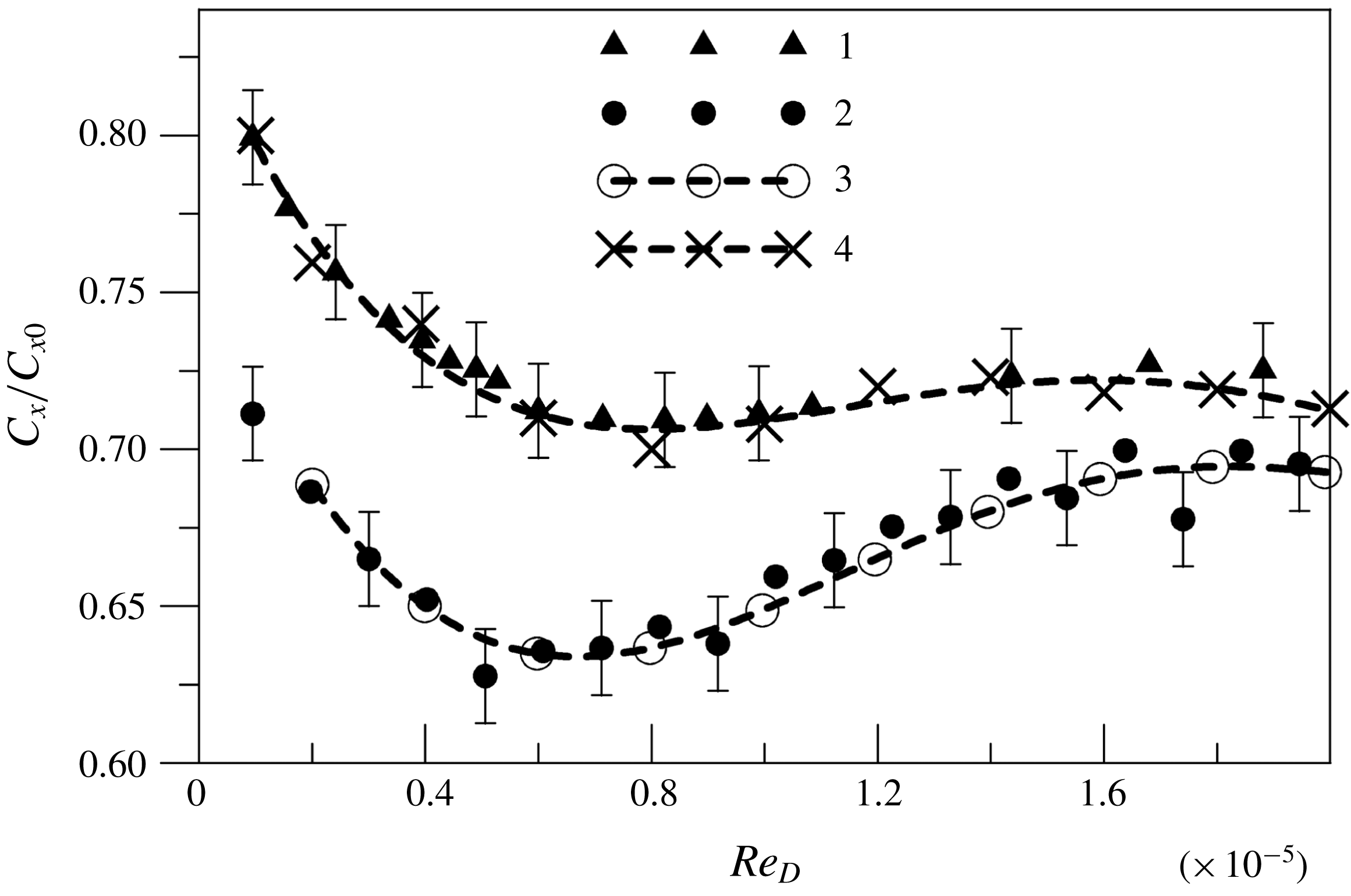
The experimental and computed normalized drag coefficients of the model,
 $C_{x}/C_{x0}$
, as functions of the Reynolds number
 $Re_{D}$
based on the free-stream parameters and the cylinder diameter
 $D$
are compared in figure 11. The experimental dependences are given for the gas-permeable inserts of length
 $\unicode[STIX]{x0394}x/D=2$
with the pore diameter
 $d=1$
and 3 mm. Figure 11 also shows the curves predicted by the skeleton model for
 $d=1$
and 3 mm and the data computed by the continuum model (Mironov et al.
Reference Mironov, Maslov, Poplavskaya and Kirilovskiy2015a
) for
 $d=3$
mm. The Reynolds number in the computations was varied by changing the free-stream static pressure calculated on the basis of the experimentally measured stagnation pressure. It is seen that the experimental and numerical data are in good agreement for both pore diameters. The results show that a 10-fold increase in the Reynolds number
 $Re_{D}$
leads to a minor (within 11 %) change in the normalized drag coefficient. This fact testifies to a weak sensitivity of the problem on viscosity in the examined range of test conditions. Thus, an inviscid flow around the HPCM skeleton prevails at supersonic velocities of the flow around the cylinder with the frontal porous insert. This fact is consistent with observations of Mironov et al. (Reference Mironov, Maslov, Poplavskaya and Kirilovskiy2015a
), which demonstrated that the flow field in the porous material and, correspondingly, the drag coefficient of the cylinder with the frontal porous insert are basically determined by the inertial (quadratic) term in the Darcy–Forchheimer law.
The drag coefficients for the solid cylinder and for the cylinder with the frontal porous insert of length
 $\unicode[STIX]{x0394}x/D=2$
for different values of
 $Re_{D}$
are listed in table 4. It is seen that the change in the drag coefficient of the cylinder with the porous insert in the considered range of the Reynolds numbers is somewhat greater (11 %) than that for the solid cylinder (4.6 %). Apparently, the friction forces on the elements of the porous insert skeleton are greater than the friction forces on the solid cylinder.
Normalized drag coefficient of the cylinder versus the normalized length of the porous insert: (1,2) cylinder
 $D=14.5$
mm with an aerospike at (1)
 $M_{\infty }=4.85$
and
 $Re_{1\infty }=2.7\times 10^{6}~\text{m}^{-1}$
and (2)
 $M_{\infty }=7$
and
 $Re_{1\infty }=1.5\times 10^{6}~\text{m}^{-1}$
; (3,4) cylinder
 $D=14.5$
mm with a frontal porous insert
 $d=3$
mm at (3)
 $M_{\infty }=4.85$
and
 $Re_{1\infty }=2.7\times 10^{6}~\text{m}^{-1}$
and (4)
 $M_{\infty }=7$
and
 $Re_{1\infty }=1.5\times 10^{6}~\text{m}^{-1}$
; (5) cylinder
 $D=34$
mm with a frontal porous insert
 $d=3$
mm at
 $M_{\infty }=21$
and
 $Re_{1\infty }=0.6\times 10^{6}~\text{m}^{-1}$
.

Drag coefficients of the solid cylinder and the cylinder with the frontal porous insert with
 $D=14.5$
mm,
 $d=1$
mm,
 $\unicode[STIX]{x0394}x/D=2$
,
 $L=100$
mm,
 $M_{\infty }=4.85$
.

For determining the effect of the Mach number, we measured the drag force of a cylinder with frontal porous inserts and a cylinder with a blunted aerospike for various Mach numbers. The data of these measurements are depicted in figure 12. It is seen that the normalized drag coefficient increases with increasing Mach number both for the cylinder with the frontal porous insert and for the cylinder with the aerospike. A similar trend is observed for models with other values of the cylinder diameter and pore diameter in the frontal gas-permeable inserts. It should be noted that the cylinder with a blunted aerospike has a lower drag coefficient than the cylinder with the frontal gas-permeable insert. However, in the case of flow control with the use of the aerospike, intense self-sustained oscillations arise at the spike lengths
 $\unicode[STIX]{x0394}x/D=0.5{-}1.5$
owing to the emergence of high-amplitude pulsations in the frontal unsteady separation region (see Zapryagaev & Mironov (Reference Zapryagaev and Mironov1989)). As a result, the vehicle experiences high dynamic loads. Such an unsteady flow is not observed in the case of flow control with the use of the frontal porous insert.
The normalized drag coefficient for a cylinder with a long HPCM insert (
 $\unicode[STIX]{x0394}x/D=2$
) was computed for the Mach numbers 4.85 and 7. The results of these calculations are listed in table 5. It is seen that the computed and experimental data for these Mach numbers are in good agreement.
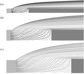
Streamlines in the normal direction to the
 $x$
axis for the flow around a cylinder with a porous insert with
 $d=1$
mm,
 $M_{\infty }=7$
,
 $p_{\infty }=186$
Pa,
 $T_{\infty }=51$
K,
 $Re_{1\infty }=2.7\times 10^{6}~\text{m}^{-1}$
: (a)
 $D=6$
mm; (b)
 $D=14.5$
mm; (c)
 $D=20$
mm.

Normalized drag coefficients for a cylinder with
 $D=14.5$
mm and a frontal HPCM insert (
 $\unicode[STIX]{x0394}x/D=2$
).

Figure 13 shows the streamlines for the flow around cylinders of different diameters
 $D=6$
, 14.5 and 20 mm with a frontal porous insert of length
 $\unicode[STIX]{x0394}x/D=2$
and HPCM cell diameter
 $d=1$
mm for
 $M_{\infty }=7$
. It is seen that the angle of streamline deviation from the model surface increases with increasing model diameter, which is caused by more intense gas exhaustion from the porous region having a greater diameter. An increase in the angle of deflection of the streamlines leads to an increase in the slope of the shock wave and its intensity, which, in turn, results in an increase in the wave drag of the large-diameter cylinder with the frontal porous insert.
It is seen in figure 13 that the flow passing through the peripheral part of the insert face interacts with a small number of skeleton elements in the streamwise and transverse directions and rapidly leaves the porous region. If the impinging flow passes through the central (axial) part of the porous insert, it interacts with a greater number of skeleton elements in the streamwise and transverse directions, i.e. the total pressure loss in this region is significantly greater than those in the peripheral region (blockage effect of the central part of the porous region). An increase in the model diameter
 $D$
with an unchanged pore diameter
 $d$
leads to a relative increase in the fraction of the central part of the porous insert and, as a consequence, to an increase in the total drag of the model. It should be noted that an increase in the pore diameter
 $d$
corresponds to a smaller number of skeleton elements, thus resulting in a smaller total pressure loss on these elements. In turn, these factors reduce the total drag of the model. Thus, an increase in the model diameter
 $D$
and an increase in the pore diameter
 $d$
lead to opposite effects.
Figure 14 shows the experimental curves of the normalized drag coefficient
 $C_{x}/C_{x0}$
as functions of the normalized length of the porous insert for different HPCM pore diameters and different cylinder diameters
 $D=24$
mm and 34 mm. Similar dependences for
 $D=14.5$
mm are presented in figure 10. It is seen that the normalized drag coefficient increases with an increase in the cylinder diameter; vice versa, an increase in the pore diameter leads to reduction of the normalized drag coefficient.
Normalized drag coefficient of cylinders with diameters
 $D=24$
mm (a) and 34 mm (b) versus the normalized length of the porous insert:
 $M_{\infty }=7$
,
 $Re_{1\infty }=1.5\times 10^{6}~\text{m}^{-1}$
, and
 $d=1$
mm (1), 2 mm (2), 3 mm (3), and 4 mm (4).

Figure 15 shows the experimental and computed values of the normalized drag coefficient
 $C_{x}/C_{x0}$
as functions of the ratio
 $D/d$
. These data were obtained for the normalized length of the porous insert, where the ratio
 $C_{x}/C_{x0}$
reaches a constant minimum value. The minimum value is reached at
 $\unicode[STIX]{x0394}x/D\geqslant 2$
for
 $D=14.5$
mm and 24 mm and at
 $\unicode[STIX]{x0394}x/D\geqslant 1.5$
for
 $D=34$
mm (see figures 10 and 14). It is seen in figure 15 that the drag coefficient increases with increasing
 $D/d$
. The computed and experimental data agree within the measurement accuracy. The observed scatter of the computed data is caused by the discrete nature of the skeleton model.
Computed and experimental values of the normalized drag coefficient of a cylinder with a porous insert versus the ratio of the model diameter to the pore diameter: (1) experiment at
 $M_{\infty }=4.85$
and
 $Re_{1\infty }=2.7\times 10^{6}~\text{m}^{-1}$
; (2) experiment at
 $M_{\infty }=7$
and
 $Re_{1\infty }=1.5\times 10^{6}~\text{m}^{-1}$
; (3) experiment at
 $M_{\infty }=21$
and
 $Re_{1\infty }=6\times 10^{5}~\text{m}^{-1}$
; (4,5) computed data for
 $M_{\infty }=4.85$
,
 $Re_{1\infty }=2.7\times 10^{6}~\text{m}^{-1}$
and
 $Re_{1\infty }=6.9\times 10^{6}~\text{m}^{-1}$
, respectively; (6,7) computed data for
 $M_{\infty }=7$
,
 $Re_{1\infty }=2.7\times 10^{6}~\text{m}^{-1}$
and
 $Re_{1\infty }=1.5\times 10^{6}~\text{m}^{-1}$
, respectively; (8,9,10) approximation dependence (5.1).

The experimental and numerical data in figure 15 are approximated by a unified dependence
 $$\begin{eqnarray}\frac{C_{x}}{C_{x0}}=1-\frac{2.525}{\sqrt{D/d}}\,M_{\infty }^{-2/3}.\end{eqnarray}$$
Figure 15 and equation (5.1) reveal the dependence of all experimental and computed data for the normalized drag coefficient as a function of the ratio of the cylinder diameter to the pore diameter for different Mach numbers in a wide range of Reynolds numbers
 $Re_{1\infty }$
from
 $1.4\times 10^{6}~\text{m}^{-1}$
to
 $1.4\times 10^{7}~\text{m}^{-1}$
. The combined information for all computed and experimental data (including the cylinder with the aerospike) is available in figure 16, which shows the linear dependences of the normalized drag coefficient on the parameter
 $$\begin{eqnarray}(D/d)^{-1/2}M_{\infty }^{-2/3}.\end{eqnarray}$$
It is seen that all experimental and numerical data lie on one straight line. For this reason, the empirical parameter
 $(D/d)^{-1/2}M_{\infty }^{-2/3}$
can be considered as a similarity criterion for the drag coefficient of bodies with frontal porous inserts made of the HPCM. The similarity parameter does not include the Reynolds number because the normalized drag coefficients vary insignificantly in the considered range of Reynolds numbers
 $Re_{1\infty }$
(from
 $1.4\times 10^{6}~\text{m}^{-1}$
to
 $1.4\times 10^{7}~\text{m}^{-1}$
).
A possible phenomenological justification for the proposed empirical parameter
 $(D/d)^{-1/2}M_{\infty }^{-2/3}$
can be formulated as follows. The drag of a cylinder with a frontal gas-permeable insert depends on the relationship of two gas flows: the gas flow penetrating into the porous insert and then flowing out through the side surface of the insert, and the gas flow that does not penetrate into the porous region and flows around the insert as if it were a solid cylinder. The kinetic energy (
 ${\sim}\unicode[STIX]{x1D70C}u^{2}$
) of the gas leaving the porous insert is inversely proportional to the number of elements of the porous material skeleton in the way of the flow,
 $n\approx D/d$
, i.e.
 $u^{2}\sim 1/n$
. Therefore, the flow passing through the side surface of the insert depends on
 $(D/d)^{-1/2}$
. The change in the density and wave drag of the porous insert, which includes the flow around each element of the skeleton, is determined in the similarity parameter by the dependence on the Mach number.
Thus, we propose an empirical similarity criterion, which allows one to determine the drag of the model with a frontal porous insert made of the HPCM in a supersonic flow for different flow conditions and scales of the model.
Computed and experimental values of the normalized drag coefficient of a cylinder with a porous insert versus the similarity parameter (5.2): (1) experiment for a cylinder with a frontal porous insert at
 $M_{\infty }=4.85$
and
 $Re_{1\infty }=2.7\times 10^{6}~\text{m}^{-1}$
; (2) experiment at
 $M_{\infty }=7$
and
 $Re_{1\infty }=1.5\times 10^{6}~\text{m}^{-1}$
; (3) experiment at
 $M_{\infty }=21$
and
 $Re_{1\infty }=6\times 10^{5}~\text{m}^{-1}$
; (4,5) computed data at
 $M_{\infty }=4.85$
,
 $Re_{1\infty }=2.7\times 10^{6}~\text{m}^{-1}$
and
 $Re_{1\infty }=6.9\times 10^{6}~\text{m}^{-1}$
, respectively; (6,7) computed data at
 $M_{\infty }=7$
,
 $Re_{1\infty }=2.7\times 10^{6}~\text{m}^{-1}$
and
 $Re_{1\infty }=1.5\times 10^{6}~\text{m}^{-1}$
, respectively; (8,9) experiment for a cylinder with an aerospike at
 $M_{\infty }=4.85$
,
 $Re_{1\infty }=2.7\times 10^{6}~\text{m}^{-1}$
and
 $M_{\infty }=7$
,
 $Re_{1\infty }=1.5\times 10^{6}~\text{m}^{-1}$
, respectively; (10) approximation dependence (5.1).

6 Conclusions
The problem of a supersonic flow around a cylinder with a frontal gas-permeable insert made of a high-porosity cellular material is solved experimentally and numerically. Possible applications of the HPCM for control of a supersonic flow around an axisymmetric body are studied in detail.
Schlieren visualization of the flow field and drag coefficients of the model are obtained for different lengths of the porous insert, cylinder diameter and HPCM pore diameter in experiments performed in supersonic wind tunnels at flow Mach numbers of 4.85, 7 and 21 in the range of Reynolds numbers
 $Re_{1\infty }=(0.6{-}13.5)\times 10^{6}~\text{m}^{-1}$
.
In terms of numerical simulations, the previously proposed skeleton model of a high-porosity cellular material of the frontal insert in the form of a system of staggered rings of different diameters is implemented. The computed positions of the bow SW and the drag coefficients are consistent with the results of wind-tunnel experiments. Therefore, the use of this skeleton model ensures adequate reproduction of the flow in a real porous material.
Significant (within 55 %) drag reduction for large lengths of the gas-permeable porous insert (
 $\unicode[STIX]{x0394}x/D\geqslant 1.5$
) is reached.
The mechanism of drag reduction for the cylinder with the frontal gas-permeable porous insert is analysed. This mechanism includes attenuation of the bow shock wave and formation of a system of weaker shocks in the external flow behind the bow shock wave, which is equivalent to the formation of an effective pointed body possessing a smaller drag coefficient than the streamwise aligned cylinder without the frontal gas-permeable insert.
It is shown that an increase in the Mach number in the case of supersonic flows around a cylinder with a frontal porous insert leads to an increase in the normalized drag coefficient both for cylinders with a frontal porous insert and for a cylinder with an aerospike. The normalized drag coefficient increases with an increase in the cylinder diameter. On the other hand, an increase in the pore diameter leads to reduction of the normalized drag coefficient.
An empirical dependence of the normalized drag coefficient on the parameter
 $(D/d)^{-1/2}M_{\infty }^{-2/3}$
, which includes the ratio of the cylinder diameter to the pore diameter and the Mach number, is derived for supersonic (
 $M_{\infty }\geqslant 5$
) flows around cylinders with frontal porous inserts made of HPCM. This parameter was proposed as a similarity criterion in the problem of a supersonic flow around a cylinder with a frontal high-porosity cellular insert (
 $k=0.95$
).
Acknowledgement
This work was supported by the Russian Foundation for Basic Research (Project no. 19-08-00113).