1. Introduction
Turbidity currents (TCs) are widespread fluid–particle coupled events occurring in the underwater environments such as rivers, reservoirs, estuaries and the deep sea. It is driven by the horizontal pressure gradient between the TC and the ambient fluid (Simpson Reference Simpson1982; Meiburg, Radhakrishnan & Nasr-Azadani Reference Meiburg, Radhakrishnan and Nasr-Azadani2015). As TCs carry a large number of particles, they exert a significant effect on the evolution of seabed topography and the safety of submarine structures (Parker et al. Reference Parker, Garcia, Fukushima and Yu1987; Kneller & Buckee Reference Kneller and Buckee2000; Fine et al. Reference Fine, Rabinovich, Bornhold, Thomson and Kulikov2005; Carter et al. Reference Carter, Gavey, Talling and Liu2014; Meiburg et al. Reference Meiburg, Radhakrishnan and Nasr-Azadani2015). In the process of TC propagation downstream, Kelvin–Helmholtz (KH) billows are induced near the stratified upper interface due to the mutual shear with the ambient fluid, which contributes to the mixing of the two fluids (Turner Reference Turner1986). Turbulence breakdown caused by stratified shear KH instabilities is an important cause of vertical transport of mass and momentum in the TC regions (Woods Reference Woods1968; De Silva et al. Reference De Silva, Fernando, Eaton and Hebert1996; Smyth & Moum Reference Smyth and Moum2012; Rahmani et al. Reference Rahmani, Lawrence and Seymour2014a ), making it vital to the understanding of geophysical fluid dynamics (Geyer & Smith Reference Geyer and Smith1987; Tedford et al. Reference Tedford, Carpenter, Pawlowicz, Pieters and Lawrence2009; Wells & Dorrell Reference Wells and Dorrell2021; Tu et al. Reference Tu, Wu, Fan, Liu, Zhang and Smyth2024). Therefore, scholars have been carrying out lots of research on KH phenomenon in TCs using field observation (Tu et al. Reference Tu, Fan, Lian, Liu, Liu, Kaminski and Smyth2020, Reference Tu, Fan, Sun, Kaminski and Smyth2022), flume experiments (Baas et al. Reference Baas, McCaffrey, Haughton and Choux2005; Gray, Alexander & Leeder Reference Gray, Alexander and Leeder2005; Khavasi & Firoozabadi Reference Khavasi and Firoozabadi2018), theoretical analysis (Harang et al. Reference Harang, Thual, Brancher and Bonometti2014; Khavasi & Firoozabadi Reference Khavasi and Firoozabadi2019) and numerical simulations (Jackson, Hallberg & Legg Reference Jackson, Hallberg and Legg2008; Kostaschuk et al. Reference Kostaschuk, Nasr‐Azadani, Meiburg, Wei, Chen, Negretti, Best, Peakall and Parsons2018; Lee Reference Lee2019).
It is generally recognised that KH billows are triggered by the redistribution of initial vortex sheet vorticity and the accumulation of vorticity in the billow core (Corcos & Sherman Reference Corcos and Sherman1976). Early KH billows manifest a series of periodic spanwise vortices, which cause the density interface to be rolled up. In weak stratification, periodic vortices will gradually merge into two or more vortices rotating around each other (Winant & Browand Reference Winant and Browand1974). Billow structures are very vulnerable to secondary three-dimensional instabilities, and the vorticity braids, produced from the billow cores, go to a subsequent breakdown of secondary, spanwise-periodic streamwise-aligned vortices (Caulfield & Peltier Reference Caulfield and Peltier2000; Mashayek & Peltier Reference Mashayek and Peltier2012a ). In the laboratory experiment, numerous new vortices are observed downstream in the flow field (Corcos & Sherman Reference Corcos and Sherman1976). It is distinct from the numerical simulation where the flow eventually returns to a laminar state due to viscous dissipation (Caulfield & Peltier Reference Caulfield and Peltier2000; Carpenter, Lawrence & Smyth Reference Carpenter, Lawrence and Smyth2007; Smyth, Carpenter & Lawrence Reference Smyth, Carpenter and Lawrence2007; Rahmani et al. Reference Rahmani, Lawrence and Seymour2014a ). There is a consensus regarding KH billows, specifically that large-scale motions are responsible for entrainment, while small-scale structures are responsible for mixing (Dimotakis Reference Dimotakis2000; Carpenter et al. Reference Carpenter, Lawrence and Smyth2007; Rahmani et al. Reference Rahmani, Lawrence and Seymour2014a ; Yang et al. Reference Yang, Timmermans and Lawrence2024a ).
The KH instability often occurs when both interface thicknesses of particle concentration (density) and velocity are close to each other. In stratified shear flows, including TC flows, Holmboe instability occurs when the particle concentration (density) interface is thinner than the velocity interface, manifesting as cusp-like internal waves (Holmboe Reference Holmboe1962; Browand & Winant Reference Browand and Winant1973; Smyth, Klaassen & Peltier Reference Smyth, Klaassen and Peltier1988; Carpenter et al. Reference Carpenter, Tedford, Rahmani and Lawrence2010). This instability is considered to be one of the keys to stimulating small-scale mixing. The KH instability and Holmboe instability often occur simultaneously in natural TC flows, making TC dynamics more complicated. The coincidence of the centre of the particle concentration interface and the centre of the velocity interface corresponds to a symmetric situation (see figure 1 of Yang et al. Reference Yang, Timmermans and Lawrence2024a ), and vice versa is an asymmetric configuration, a phenomenon commonly observed in geophysical events such as TCs (Wesson & Gregg Reference Wesson and Gregg1994; Yoshida et al. Reference Yoshida, Ohtani, Nishida and Linden1998; van Haren et al. Reference van Haren, Gostiaux, Morozov and Tarakanov2014; Tu et al. Reference Tu, Fan, Sun, Kaminski and Smyth2022). The asymmetric KH billow is identified as a hybrid mode of symmetric KH instability and Holmboe instability, which sharpens the density interface by scouring the intermediate density fluid on the upper interface (Olsthoorn, Kaminski & Robb Reference Olsthoorn, Kaminski and Robb2023; Yang et al. Reference Yang, Timmermans and Lawrence2024a ). When the velocity interface is more than twice as thick as the density interface, the asymmetric Holmboe instability exhibits a similar hybrid behaviour (Lawrence, Browand & Redekopp Reference Lawrence, Browand and Redekopp1991; Carpenter et al. Reference Carpenter, Lawrence and Smyth2007). The vortices generated by asymmetric Holmboe instability resemble those formed by KH billows (Caulfield Reference Caulfield2021).
Another important process in the dynamics of KH billows is the pairing and merging of primary two-dimensional vortices, which represents the dominant two-dimensional instability. This process, to a great extent, depends on the phase relationship between the primary mode and the subharmonic mode (Dong et al. Reference Dong, Tedford, Rahmani and Lawrence2019). Vortex pairing facilitates enhanced mixing (Rahmani et al. Reference Rahmani, Seymour and Lawrence2014b ; Dong et al. Reference Dong, Tedford, Rahmani and Lawrence2019; Liu, Kaminski & Smyth Reference Liu, Kaminski and Smyth2022) by increasing the thickness of the shear layer (Corcos & Sherman Reference Corcos and Sherman1984; Xu, Stastna & Deepwell Reference Xu, Stastna and Deepwell2019). An increase in the Reynolds number inhibits vortex pairing (Salehipour et al. Reference Salehipour, Caulfield and Peltier2016a ), as it promotes the development of three-dimensional secondary instabilities that disrupt the two-dimensional coherent structures essential for vortex pairing (Mashayek & Peltier Reference Mashayek and Peltier2012a , Reference Mashayek and Peltierb ). It is interesting to explore the impact of profile structures on instability excitation modes and to study the vortex pairing mechanism in complex TC systems.
Cantero, Balachandar & Garcia (Reference Cantero, Balachandar and García2008) found that particles migrated from the KH vortex regions and accumulated in the front and the body of the TC with high shear. The existence of inertial particles would weaken the vortices due to the lag between particle and fluid velocities, which led to the reduction of the deceleration velocity (Cantero et al. Reference Cantero, Balachandar and García2008). Simpson (Reference Simpson1972) clarified the impact of convective instability on the structure of the lobe and the cleft, which was further demonstrated by Härtel et al. (Reference Härtel, Meiburg and Necker2000a , Reference Härtel, Carlsson and Thunblomb ) and Horner-Devine & Chickadel (Reference Horner‐Devine and Chickadel2017). Lee (Reference Lee2019) drew attention to the relationship between the KH vortices and the TC dilution mechanism as well as the pattern of interaction forces within the vortices, namely that the buoyancy force is centripetal and the drag force exhibits a pattern of pointing towards a position higher than the vortex. Small particles will remain in the core of the vortex, where there is no vorticity, leading to local high concentrations. Although the evolution of KH billows in TCs has been extensively explored, the coupling regimes between particle action and the KH billows within the TC process need to be fully understood, especially in respect to the individual particle motion behaviour. This helps us further clarify the mixing mechanism of TCs with ambient fluids and the dynamics of TC advancement.
It is of interest to explore the critical conditions for inducing KH billows in TCs. The prevailing cognition is to use the Richardson number
 $Ri$
, which represents the ratio of the buoyancy term to the flow shear term, as the judgment factor (Miles Reference Miles1961; Turner Reference Turner1986; Harang et al. Reference Harang, Thual, Brancher and Bonometti2014). Kelvin–Helmholtz billows start to develop when the fluid shear is stronger than the stability promoted by density stratification. Thus, the Richardson number has been widely adopted to estimate the TC entrainment (Turner Reference Turner1986; Parker et al. Reference Parker, Garcia, Fukushima and Yu1987; Lombardi et al. Reference Lombardi, Adduce and La Rocca2018). There are two forms of Richardson number, the bulk Richardson number
 $Ri_0$
and the gradient Richardson number
 $Ri_g$
, which are respectively expressed by
 \begin{align}&\,\, Ri_0 = \frac {g_m^{\prime} h \cos \theta }{\bar {U}^2}, \end{align}
 \begin{align}& Ri_g = -\frac {|\boldsymbol{g}| \dfrac {\partial \rho _m}{\partial z}}{\rho _f \left(\dfrac {\partial U}{\partial z}\right)^2}, \end{align}
where
 $g_m^{\prime} = g' \bar {\alpha _p}$
is the effective gravitational acceleration of the fluid–particle mixture with
 $g'=|\boldsymbol{g}|(\rho _p-\rho _f)/\rho _f$
being the particle effective gravitational acceleration and
 $\bar {\alpha _p}$
being the depth-averaged particle volumetric fraction of the current,
 $\boldsymbol{g}$
is the gravitational acceleration,
 $\rho _f$
,
 $\rho _p$
and
 $\rho _m$
are the densities of the fluid, particle and mixture, respectively;
 $h$
denotes the current height,
 $\theta$
is the angle of slope and
 $\bar {U}$
is the depth-averaged value of the current velocity
 $U$
. Miles (Reference Miles1961) and Howard (Reference Howard1961) demonstrated that for a gradient Richardson number,
 $Ri_g \gt 0.25$
is sufficient for the stability of an inviscid, incompressible and heterogeneous shear flow, which was first derived by Taylor (Reference Taylor1931). This threshold indicates the critical point at which the destabilising effects of flow shear surpass the stabilising effects of stratification. Subsequently, numerous studies have applied this threshold to analyse TC instability, despite the viscous nature of a TC and the complexities introduced by particle dynamics (Tedford et al. Reference Tedford, Carpenter, Pawlowicz, Pieters and Lawrence2009; Harang et al. Reference Harang, Thual, Brancher and Bonometti2014; Kneller et al. Reference Kneller, Nasr-Azadani, Radhakrishnan and Meiburg2016). Turner (Reference Turner1986) suggested that the flows at the condition of the bulk Richardson number above 0.8 were stable. The fundamental tenet of this paradigm is the unification of fluid–particle mixtures. It makes sense to investigate the distinct characteristics of each phase in turn when talking about fluids and particles separately. Among these, the fluid and particle velocity gradients, which stand for the viscosity brought on by fluid shear and the damping brought on by particle collision, respectively, govern the shear term
 $\rho _f (\partial U / \partial z)^2$
. Particle damping plays a significant role in TCs at high particle volume fractions. For TCs with low particle volume fractions, the mixture’s velocity gradient
 $\partial U / \partial z$
is nearly equal to the streamwise fluid velocity gradient
 $\partial u_{\!f} / \partial z$
, i.e.
 $\partial U / \partial z \approx \partial u_{\!f} / \partial z$
. This velocity gradient is directly associated with the vertical Saffman lift experienced by the particle that contributes to its roll-up (Saffman Reference Saffman1965; Xie et al. Reference Xie, Hu, Pähtz, He and Cheng2023a
). It is simple to infer that the fluid longitudinal velocity and the KH billows formed by the particles in the TC have a significant correlation. The relationship between the Richardson number, particle motion, various fluid forces acting on the particles and KH billow occurrence conditions has not been thoroughly investigated as of yet.
The TC’s advancing and mixing regimes are both influenced by the flow Reynolds number
 ${\textit{Re}}$
, which is defined as
 \begin{equation} {Re} = \frac {\rho _f u_b L_c}{{\mu} _f}, \end{equation}
where
 $L_c$
is the characteristic length, which is typically defined as the current front height during the TC slumping phase. Specifically, in the case of a lock-exchange TC,
 $L_c$
is equal to half of the initial height of the fluid–particle mixture (Necker et al. Reference Necker, Härtel, Kleiser and Meiburg2002). Here
 $u_b$
is the buoyancy velocity that is given by (Necker et al. Reference Necker, Härtel, Kleiser and Meiburg2005; Nasr-Azadani & Meiburg Reference Nasr-Azadani and Meiburg2014; Pelmard, Norris & Friedrich Reference Pelmard, Norris and Friedrich2020)
 \begin{equation} u_b=\sqrt { \frac {\alpha _{p0}|\boldsymbol{g}|(\rho _p-\rho _f) L_c}{\rho _f}}, \end{equation}
where
 $\alpha _{p0}$
is the initial average particle volumetric fraction in the lock region. Simpson (Reference Simpson1972) concluded from the experiments that the lifting height of the nose is related to the Reynolds number and density flow height, and the relationship between the lobe width and the Reynolds number. The TC with a low Reynolds number propagates at a smaller velocity in the constant velocity phase than the TC with a high Reynolds number (Cantero et al. Reference Cantero, Lee, Balachandar and Garcia2007; Hu et al. Reference Hu, Tao, Li and He2020). The results of Cantero et al. (Reference Cantero, Lee, Balachandar and Garcia2007) suggested that the low Reynolds number TC would directly develop from the slumping phase to viscous phase without passing through the inertial stage, agreeing with Amy et al. (Reference Amy, Hogg, Peakall and Talling2005). Simulations regarding the large Reynolds number TC demonstrated that turbulence in the near-wall region of TCs exhibits remarkable similarities to turbulence in standard wall-bounded flows, including identifiable low- and high-speed streaks and hairpin vortices (Cantero et al. Reference Cantero, Balachandar and García2008; Ooi, Constantinescu & Weber Reference Ooi, Constantinescu and Weber2009). The mixing between the ambient fluid and the gravity flow head fluid is related to the Reynolds number, which is obtained from the cube root of the buoyancy flux into the front and the flow height (Parsons & Garcia Reference Parsons and Garcia1998). Compared with the low-Reynolds-number condition, the KH billows in the high-Reynolds-number condition lose their spanwise coherence earlier, and there exist more small three-dimensional eddies near the interface that break interfacial billows into smaller turbulent structures (Ooi et al. Reference Ooi, Constantinescu and Weber2009). As the TC evolves, the KH billows near the interface and the bottom resistance together hinder the initial acceleration of the front, after which the current enters the constant velocity phase (Cantero et al. Reference Cantero, Balachandar and García2008). Currently, a general understanding of how the Reynolds number affects the TC has not been established. It has not yet been elucidated how particle motion in the mesoscopic scale responds to the macroscopic flow Reynolds number during the TC development, especially in the KH billow processes.
In contrast to our previous work (Xie et al. Reference Xie, Hu, Pähtz, He and Cheng2022, Reference Xie, Hu, Zhu, Yu and Pähtz2023a ), this study differs in the research tools employed. While large eddy simulation was used to model fluid motion in the past, this work utilises direct numerical simulation (DNS), which generates abundant data with excellent simulation accuracy and high resolution. Additionally, the discrete element method (DEM) is employed to compute particle collisions and track particle trajectories. In terms of fluid–particle coupling, this study adopts the model A derived, in detail, by Zhou et al. (Reference Zhou, Kuang, Chu and Yu2010), which is less conditional compared with the previously used simplified model B. In model A the pressure is shared by both the fluid and particle phases. The equations for the DNS-DEM model and the numerical set-ups for the lock-exchange TCs are introduced in § 2. The numerical resolution is also compared here.
Regarding research content, past works have predominantly focused on the particle suspension and transport mechanisms in TCs, including particle auto-suspension and segregation. In contrast, this study investigates the following mesoscopic-scale physical regimes regarding KH billows that occur near the interface in TC processes:
-
(i) the induction and development regime of KH billows, particularly the mutual coupling between particles and KH billows;
-
(ii) the impact of Reynolds number on the formation and growth of KH billows.
This work primarily addresses the following five areas.
-
(a) Turbidity current dynamics at moderate Reynolds numbers: while the fluid–particle coupling in lock-exchange TC at low Reynolds numbers (
 ${Re} \;{\sim}\; O(10)$
) has been studied, a gap remains in understanding the high-Reynolds-number conditions typically observed in actual geophysical flows (Meiburg et al. Reference Meiburg, Radhakrishnan and Nasr-Azadani2015). The interfacial KH instability, commonly observed in real-world TCs, is almost absent at low Reynolds numbers (Xie et al. Reference Xie, Hu, Zhu, Yu and Pähtz2023a
). The coupling between this instability and particle motion, as well as the influence of Reynolds number on both, requires further exploration. Due to the increased computational cost associated with higher Reynolds numbers, particularly the greater number of particles involved, we aim to investigate the dynamics of TCs at moderate Reynolds numbers (
${Re} \;{\sim}\; O(10^3)$
). A revisit of the lock-exchange TC process and a preliminary investigation of the effect of Reynolds number are given in § 3.
-
(b) Effect of spanwise length on KH billow evolution: our focus lies in the evolution of the primary two-dimensional KH billows. Considering the limitation of computational cost, the simulation is three-dimensional but the computational domain width is relatively small. This may affect the development of three-dimensional small-scale structures that have a significant impact on KH billows (Caulfield & Peltier Reference Caulfield and Peltier2000; Necker et al. Reference Necker, Härtel, Kleiser and Meiburg2002; Mashayek & Peltier Reference Mashayek and Peltier2012a ). Section 4 preliminarily explores the influence of computational domain width on KH billows in TCs.
-
(c) Evolution mechanism of KH billows: a substantial body of research has focused on the interfacial instability of stratified shear flows (Caulfield Reference Caulfield2021), including investigations within TC environments (Harang et al. Reference Harang, Thual, Brancher and Bonometti2014; Kostaschuk et al. Reference Kostaschuk, Nasr‐Azadani, Meiburg, Wei, Chen, Negretti, Best, Peakall and Parsons2018). However, the mechanisms underlying the excitation and evolution of KH billows – particularly from the combined perspective of fluid dynamics and particle motion – remain insufficiently understood. This mechanism is revealed in § 5.
-
(d) Influence of KH billows on particle motion: the impact of KH billows on particle transport and deposition warrants further investigation, as it is crucial for understanding the mechanisms by which TCs carry large amounts of sediment in the real world. The relevant findings are discussed in § 6.
-
(e) Energy conversion of the TC and interface billows: interface instability is a key process for energy conversion and dissipation in TCs. Exploring the mechanisms of vortex dissipation is intriguing. Section 7 first examines the energy budget of the TC and then discusses the energy dissipation associated with the interface vortex. By decomposing the energy dissipation, we reveal the energy dissipation regime of the KH billows.


Finally, § 8 gives a summary and discussion of the work.
2. Methodology
In the paper we employ the Eulerian–Lagrangian approach to investigate the TC dynamics, especially for the coupling regimes between the particle movement and KH billows. For the fluid phase, the DNS method is adopted, whereas the DEM is utilised for the particle phase. In the following, § 2.1 gives the governing equations of the DNS-DEM model and § 2.2 describes the numerical settings of the lock-exchange TCs.
2.1. Governing equations
For DNS, the Navier–Stokes equations for the incompressible fluids are given by
 \begin{align}& \frac {\partial \alpha _f \rho _f u_{i,f}}{\partial t}+ \frac {\partial \alpha _f \rho _f u_{i,f} u_{j,f}}{\partial x_j} = -\alpha _f \frac {\partial p}{\partial x_i} + \alpha _f \rho _f g_i + \alpha _f \frac {\partial \tau _{i j}}{\partial x_j} - R_{i,p f}, \end{align}
 \begin{align}&\qquad\qquad\qquad\qquad\qquad \frac {\partial \alpha _f}{\partial t}+\frac {\partial \alpha _f u_{i,f}}{\partial x_i} = 0, \end{align}
where
 $\alpha _f = 1 - \alpha _p$
is the fluid volumetric fraction, in which
 $\alpha _p$
is the particle volumetric fraction determined by the real-time particle spatial distribution,
 $\rho _f$
is the fluid density,
 $u_{i,f}$
(
 $i=1,2,3$
) is the fluid velocity,
 $p$
is the fluid pressure,
 $g_i$
is the gravitational acceleration component,
 $\tau _{i j}$
is the fluid stress tensor and
 $R_{i, p f}$
denotes the momentum exchange term from the particle phase to the fluid, which is defined in (2.8).
The governing equations for the particle phase are based on Newton’s second law and the conservation of angular momentum, and capture the translational and rotational behaviour of particle
 $i$
:
 \begin{align}& m_i \frac {{\textrm{d}}{u}_{p,i}}{{\textrm{d}}t} = m_i \boldsymbol{g} + \boldsymbol{F}^f_i + \sum \limits _{j = 1}^{n^c_i}\boldsymbol{F}^c_{i j}, \end{align}
 \begin{align}&\qquad\quad I_i \frac {{\textrm{d}}{\omega }_{p,i}}{{\textrm{d}}t} = \sum \limits _{j = 1}^{n^c_i}\boldsymbol{M}^c_{i j}. \end{align}
Here
 $m_i$
and
 $I_i$
are the mass and the moment of inertia of the particle, respectively;
 $\boldsymbol{u}_{p,i}$
and
 $\boldsymbol{\omega }_{p,i}$
are the particle translational velocity and the particle angular velocity, respectively;
 $m_i \boldsymbol{g}$
is the particle gravity with
 $\boldsymbol{g} = (0,0,-9.81) \, \textrm{m s}^{-2}$
;
 $\boldsymbol{F}^f_i$
represents the fluid–particle interaction force acting on the particle;
 $\boldsymbol{F}^c_{i j}$
and
 $\boldsymbol{M}^c_{i j}$
are the contact force and the torque acting on particle
 $i$
by particle
 $j$
or the boundary wall, respectively; and
 $n^c_i$
represents the number of particles in interaction with particle
 $i$
. The Hertz–Mindlin model is used to solve particle–particle and particle–wall contact force
 $\boldsymbol{F}^c_{ij}$
(Cundall & Strack Reference Cundall and Strack1979), i.e.
 \begin{equation} {\boldsymbol {F}}_{ij}^c = \left ({k^n}\delta _{ij}^n - {\gamma ^n}\nu _{ij}^n\right ) + \left ({k^t}\delta _{ij}^t - {\gamma ^t}\nu _{ij}^t\right ), \end{equation}
where
 $\delta ^n_{ij}$
is the normal overlap distance,
 $\delta ^t_{ij}$
is the tangential displacement;
 $\nu ^n_{ij}$
and
 $\nu ^t_{ij}$
are, respectively, the normal and tangential relative velocities between particles;
 $k^n$
and
 $k^t$
are the normal and tangential elastic constants, respectively; and
 $\gamma ^n$
and
 $\gamma ^t$
are the normal and tangential viscoelastic damping constants, respectively. The tangential contact part, which is represented by the second component on the right-hand side of (2.5), is constrained by Coulomb’s law, i.e.
 \begin{eqnarray} {k^t}\delta _{ij}^t - {\gamma ^t}\nu _{ij}^t \leqslant {{\mu}} _c \left({k^n}\delta _{ij}^n - {\gamma ^n}\nu _{ij}^n \right), \end{eqnarray}
where
 ${{\mu}} _c=0.5$
is the friction coefficient. We employ a Young’s modulus
 $Y=5\times 10^6$
Pa, Poisson ratio
 $\nu =0.45$
and coefficient of restitution
 $e=0.3$
to determine these constants pertaining to the contact force model, the values of which are the same as those in our previous studies (Xie et al. Reference Xie, Hu, Zhu, Yu and Pähtz2023a
,
Reference Xie, Zhu, Hu, Yu and Panb
).
As the particle diameter
 ${\textrm{d}}_p$
is much smaller than the Kolmogorov length scale
 $\eta$
in this TC work (
 ${\textrm{d}}_p/\eta \ll O(1)$
, where
 $\eta$
is of the order of
 $O(10^{-3}\;{\sim}\; 10^{-2})$
m), the particle modulation on turbulence can be disregarded (Balachandar Reference Balachandar2009). Taking this into consideration, we model the fluid–particle interaction using the point-force hypothesis. The fluid force in this framework is configured to be applied to the particle’s centre of mass. The force of the particle on a given fluid grid is determined by the ratio of the volume of the particle in the grid to the volume of the particle (Jing et al. Reference Jing, Kwok, Leung and Sobral2016). Given that an increase in the Reynolds number typically corresponds to greater flow complexity, we employ here model A, as theoretically derived by Zhou et al. (Reference Zhou, Kuang, Chu and Yu2010), to calculate fluid–particle interactions. In coupling implementation, the fluid–particle interaction force
 $\boldsymbol{F}^f$
includes drag force
 $\boldsymbol{F}^d$
, pressure gradient force
 $\boldsymbol{F}^{\boldsymbol\nabla p}$
, viscous force
 $\boldsymbol{F}^{\boldsymbol\nabla \boldsymbol\cdot \boldsymbol{\tau }}$
, lift force
 $\boldsymbol{F}^l$
and added mass force
 $\boldsymbol{F}^{\textit{add}}$
. The fluid–particle interaction force on an individual particle
 $i$
can be presented as
 \begin{eqnarray} \boldsymbol{F}^f_i = \boldsymbol{F}^d_i + \boldsymbol{F}^{\boldsymbol\nabla p}_i + \boldsymbol{F}^{\boldsymbol\nabla \boldsymbol\cdot \boldsymbol{\tau }}_i + \boldsymbol{F}^l_i + \boldsymbol{F}^{\textit{add}}_i. \end{eqnarray}
The coupling strategy of model A must incorporate both the pressure gradient force and the viscous force (Kafui, Thornton & Adams Reference Kafui, Thornton and Adams2002; Zhou et al. Reference Zhou, Kuang, Chu and Yu2010). Along with the drag force, these are considered the primary force components in fluid–particle flow (Zhou et al. Reference Zhou, Kuang, Chu and Yu2010). For the entire TC flow, the drag force and pressure gradient force significantly impede particle sedimentation (Lee Reference Lee2019; Xie et al. Reference Xie, Hu, Pähtz, He and Cheng2022); the lift force and added mass force are essential for promoting the auto-suspension of the TC head (Xie et al. Reference Xie, Hu, Zhu, Yu and Pähtz2023a
). Thus, this work accounts for these force components. Compared with the Maxey–Riley–Gatignol equation for particle motion (Gatignol Reference Gatignol1983; Maxey & Riley Reference Maxey and Riley1983), the Basset history force is neglected. This omission arises because the Basset force is computationally challenging to determine and analytically difficult to incorporate (Schmeeckle Reference Schmeeckle2014; Pähtz et al. Reference Pähtz, Liu, Xia, Hu, He and Tholen2021). Quantifying these forces helped us better understand the KH billows excitation (figures 16 and 17) and pairing mechanisms (figures 20 and 31) at the TC interface. The volumetric fluid–particle interaction term
 $\boldsymbol{R}_{p f}$
in (2.1) does not encompass the pressure gradient force and viscous force, which have already been accounted for in the pressure gradient term and viscous term, respectively, of (2.1).Therefore, the momentum exchange term
 $\boldsymbol{R}_{p f}$
is determined by
 \begin{equation} {\boldsymbol{R}_{pf}} = \frac {1}{V_{cell}} {\sum \limits _{\zeta = 1}^{k_c}} {\Big( {\boldsymbol {F}}_\zeta ^f - {\boldsymbol {F}}_\zeta ^{\boldsymbol\nabla p} - {\boldsymbol {F}}_\zeta ^{\boldsymbol\nabla \boldsymbol\cdot \boldsymbol{\tau }} \Big) } = \frac {1}{V_{cell}}{\sum \limits _{\zeta = 1}^{{k_c}} {\big( {\boldsymbol {F}}_\zeta ^d + {\boldsymbol {F}}_\zeta ^l + {\boldsymbol {F}}_\zeta ^{\textit{add}}\big)} }, \end{equation}
where
 $V_{cell}$
is the cell volume of fluid simulation and
 $k_c$
is the number of particles located in the corresponding cell. Compared with our previous TC model (Xie et al. Reference Xie, Hu, Zhu, Yu and Pähtz2023a
,
Reference Xie, Zhu, Hu, Yu and Panb
), this model employs a different approach to modelling the pressure gradient force based on the local
 $\boldsymbol\nabla p$
, deviating from the previously used Archimedes buoyancy model. Additionally, it introduces the viscous force. Zhou et al. (Reference Zhou, Kuang, Chu and Yu2010) pointed out that such a model framework exhibits broader adaptability, particularly for complex flow systems.
The pressure gradient force
 $\boldsymbol{F}^{\boldsymbol\nabla p}$
is formulated as
 \begin{eqnarray} \boldsymbol{F}^{\boldsymbol\nabla p} = \frac {1}{6} \pi {\textrm{d}}_p^{3} \boldsymbol\nabla p. \end{eqnarray}
For the purpose of the following analysis, we decompose the pressure gradient force into the dynamic pressure part and the hydrostatic part. The hydrostatic part,
 $\boldsymbol{F}^b$
, is calculated as
 \begin{eqnarray} \boldsymbol{F}^b=-\frac {1}{6}\pi \rho _f {\textrm{d}}_p ^3 \boldsymbol{g}. \end{eqnarray}
Thus, the dynamic pressure part,
 $\boldsymbol{F}^{q}$
, can be obtained by
 \begin{eqnarray} \boldsymbol{F}^q=\boldsymbol{F}^{\boldsymbol\nabla p} - \boldsymbol{F}^b = \frac {1}{6}\pi {\textrm{d}}_p ^3 (\boldsymbol\nabla p + \rho _f \boldsymbol{g}). \end{eqnarray}
Unless otherwise specified in later discussion, the buoyancy force refers to the hydrostatic part and the pressure gradient force refers to the dynamic pressure part. The viscous force
 $\boldsymbol{F}^{\boldsymbol\nabla \boldsymbol\cdot \boldsymbol{\tau }}$
, induced due to the fluid shear stress tensor, is determined by
 \begin{equation} \boldsymbol{F}^{\boldsymbol\nabla \boldsymbol\cdot \boldsymbol{\tau }} = \frac {1}{6} \pi {\textrm{d}}_p^{3} \boldsymbol\nabla \boldsymbol\cdot \boldsymbol{\tau }. \end{equation}
The drag force
 $\boldsymbol{F}^d$
can be written as (Di Felice Reference Di Felice1994; Zhao & Shan Reference Zhao and Shan2013; Jing et al. Reference Jing, Kwok, Leung and Sobral2016)
 \begin{equation} \boldsymbol{F}^d=\frac {1}{8} C_D \rho _f \pi {\textrm{d}}_p ^2 ( \boldsymbol{u}_f - \boldsymbol{u}_p )|\boldsymbol{u}_f - \boldsymbol{u}_p| \alpha _f ^{2-\chi }, \end{equation}
where
 ${\textrm{d}}_p$
is the particle diameter and
 $C_D$
is the drag coefficient that is given by
 \begin{eqnarray} C_D = \left (0.63+\frac {4.8}{\sqrt {\alpha _f {Re}_p}} \right )^2, \end{eqnarray}
where
 ${Re}_p$
is the particle Reynolds number determined as
 \begin{equation} {Re}_p = \frac {\rho _f {\textrm{d}}_p |\boldsymbol{u}_f - \boldsymbol{u}_p|}{{{\mu}} _f} , \end{equation}
in which
 ${{\mu}} _f$
is the fluid dynamic viscosity. In (2.13),
 $\chi$
is the correction factor obtained by
 \begin{eqnarray} \chi = 3.7 -0.65 \,\textrm{exp}\left [ -\frac {\left ( 1.5-\textrm{log}_{10}\left (\alpha _f {Re}_p \right ) \right )^2}{2} \right ]. \end{eqnarray}
The lift force
 $\boldsymbol{F}^l$
is modelled as (Loth & Dorgan Reference Loth and Dorgan2009)
 \begin{equation} \boldsymbol{F}^l=\frac {1}{8} C_L \rho _f \pi {\textrm{d}}_p ^2 |\boldsymbol{u}_f - \boldsymbol{u}_p| \left [ \left ( \boldsymbol{u}_f - \boldsymbol{u}_p \right ) \times \frac {\boldsymbol{\omega }_f}{|\boldsymbol{\omega }_f|} \right ], \end{equation}
with
 $\boldsymbol{\omega }_f$
representing the fluid vorticity and
 $C_L$
being the lift coefficient. In order to include the effects of both fluid vorticity and particle rotation on lift (Saffman lift and Magnus lift), the lift coefficient
 $C_L$
is expressed as (McLaughlin Reference McLaughlin1991; Loth & Dorgan Reference Loth and Dorgan2009)
 \begin{equation} C_L=J^{\ast }\frac {12.92}{\pi }\sqrt {\frac {\omega ^\ast }{{Re}_p}} + \Omega ^\ast _{p,e q} C^\ast _{L,\Omega }, \end{equation}
where
 $\omega ^\ast =|\boldsymbol{\omega }_f|{\textrm{d}}_p / |\boldsymbol{u}_f - \boldsymbol{u}_p|$
. The function
 $J^\ast$
reads (Mei Reference Mei1992; Loth & Dorgan Reference Loth and Dorgan2009)
 \begin{equation} J^\ast = 0.3 \left \{ 1 + \tanh \left [ \frac {5}{2} \left ( \textrm{log}_{10}\sqrt {\frac {\omega ^\ast }{{Re}_p}} + 0.191 \right ) \right ] \right \} \left \{ \frac {2}{3} + \tanh \left [ 6 \sqrt {\frac {\omega ^\ast }{{Re}_p}}\right ] \right \}\!. \end{equation}
Two parameters in (2.18),
 $C^\ast _{L,\Omega }$
, and
 $\Omega ^\ast _{p,eq}$
, are given as (Loth & Dorgan Reference Loth and Dorgan2009)
 \begin{align}&\qquad\quad \Omega ^\ast _{p,e q}=\frac {\omega ^\ast }{2}( 1-0.0075{Re}_\omega ) \big( 1-0.062\sqrt {{Re}_p} - 0.001{Re}_p \big), \end{align}
 \begin{align}& C^\ast _{L,\Omega } = 1 - \{ 0.675 + 0.15( 1+\tanh [0.28 (\Omega ^\ast _p-2)])\} \tanh \big[0.18 \sqrt {{Re}_p} \big], \end{align}
with
 ${Re}_\omega =\rho _f |\boldsymbol{\omega }_f|{\textrm{d}}_p ^2 / {{\mu}} _f$
and
 $\Omega ^\ast _p = |\boldsymbol{\omega }_p|{\textrm{d}}_p/|\boldsymbol{u}_f - \boldsymbol{u}_p|$
.
The added mass force
 $\boldsymbol{F}^{\textit{add}}$
is written as
 \begin{equation} \boldsymbol{F}^{\textit{add}} = \frac {1}{6}C_{\textit{add}}\rho _f \pi {\textrm{d}}_p ^2 \left ( \frac {D\boldsymbol{u}_f}{D t} - \frac {D\boldsymbol{u}_p}{D t} \right ), \end{equation}
where
 $C_{\textit{add}}=0.5$
is the added mass coefficient.
In this DNS-DEM coupling model, the open source code library OpenFOAM is employed for fluid simulation, the particle movement is solved based on LIGGGHTS, and the coupling process of the two refers to Kloss et al. (Reference Kloss, Goniva, Hager, Amberger and Pirker2012). Such a model framework has been widely used in the simulation of fluidised beds (Alobaid, Ströhle & Epple Reference Alobaid, Ströhle and Epple2013; Liu & van Wachem Reference Liu and van Wachem2019; Wang et al. Reference Wang, Luo, Hu, Lin and Fan2019; Liu, Deen & Tang Reference Liu, Deen and Tang2021), sediment transport (Schmeeckle Reference Schmeeckle2014; Sun & Xiao Reference Sun and Xiao2016; Pähtz et al. Reference Pähtz, Liu, Xia, Hu, He and Tholen2021; Nie, Wang & Yan Reference Nie, Wang and Yan2024), etc., and has been well verified.
2.2. Numerical set-up
Schematic view of the lock-exchange TC.

In this study the simulation of the lock-exchange TC is carried out in a cuboid tank, as shown in figure 1. The longitudinal (
 $x$
), transverse (
 $y$
) and vertical (
 $z$
) dimensions of the tank are
 $L_x = 0.8$
m,
 $L_y=0.02{\;{\sim}\;} 0.08$
m and
 $L_z = 0.2$
m, respectively. The tank is filled with a fluid having a density of 1000
 $\textrm {kg} \, \textrm {m}^{-3}$
and a kinematic viscosity of
 $10^{-6} \, \textrm {m}^2 \, \textrm {s}^{-1}$
. At the beginning, particles with a density of
 $\rho _p$
= 1600
 $\textrm {kg} \, \textrm {m}^{-3}$
, a particle diameter of
 ${\textrm{d}}_p = 1 \times 10^{-4}$
m and a total number of particles,
 $N_p$
, are randomly and evenly arranged on the left of the gate, which is the lock region with a longitudinal (
 $x$
) dimension of
 $L_g = 0.05$
m. The aspect ratio
 $L_z / L_g$
of initial fluid–particle mixture column is 4. The average particle volumetric fraction in the lock region is given by
 $\alpha _{p0} = N_p \pi {\textrm{d}}_p^3/(6 L_g L_y L_z)$
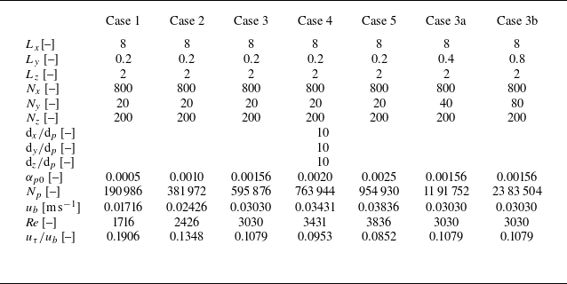
, the values of which for all cases are presented in table 1.
Computational domain dimensions (
 $L_x$
,
 $L_y$
and
 $L_z$
), grid resolution (
 $N_x$
,
 $N_y$
and
 $N_z$
), grid sizes (
 ${\textrm{d}}_x/{\textrm{d}}_p$
,
 ${\textrm{d}}_y/{\textrm{d}}_p$
and
 ${\textrm{d}}_z/{\textrm{d}}_p$
), initial particle volume fraction (
 $\alpha _{p0}$
), particle number (
 $N_p$
), buoyancy velocity (
 $u_b$
), flow Reynolds number (
 ${\textit{Re}}$
) and particle terminal velocity (
 $u_\tau /u_b$
) for the simulated cases.

In the simulation of fluids, the two longitudinal surfaces and the bottom surface of the cuboid computational domain are set as wall boundaries (no-slip boundaries), while the upper boundary is set as a slip boundary. Two transverse surfaces are assigned periodic boundaries. For the particle phase, solid boundaries are applied to the longitudinal and vertical surfaces to prevent particles from entering and exiting the computational domain, and the transverse surfaces adopt periodic boundaries, consistent with the fluid simulation. The gate is lifted immediately as soon as the simulation starts, and the particles settle under the control of gravity and form the TC that propagates downstream.
The properties of TC are described by a few parameters. The ratio of inertia to viscosity of the TC is represented by the flow Reynolds number
 ${\textit{Re}}$
, which is defined in (1.3). The gradient Richardson number
 $Ri_g$
is given by (1.2). The interfacial shear Reynolds number
 ${Re}_I$
is calculated by (Carpenter et al. Reference Carpenter, Lawrence and Smyth2007; Liu, Kaminski & Smyth Reference Liu, Kaminski and Smyth2024; Yang et al. Reference Yang, Timmermans and Lawrence2024a
)
 \begin{equation} {Re}_I = \frac {\Delta u_{f,I} h_I}{\nu }, \end{equation}
where
 $\Delta u_{f,I}$
represents the velocity jump between the TC and the ambient fluid (see figure 1 of Yang et al. Reference Yang, Timmermans and Lawrence2024a
), and
 $h_I$
represents the corresponding vertical distance. The ratio of particle density to fluid density
 $s=\rho _p/\rho _f$
is 1.6. The particle Reynolds number defined by (2.15) is of the order of
 $O(10^{-4} \;{\sim}\; 10^{-1})$
, and the particle Stokes number
 $St = s \rho _f |\boldsymbol{u}_f - \boldsymbol{u}_p|{\textrm{d}}_p/(9{{\mu}} _f)$
is of the order of
 $O(10^{-5} \;{\sim}\; 10^{-2})$
. The particle terminal velocity
 $u_\tau = (\rho _p-\rho _f)|\boldsymbol{g}|{\textrm{d}}_p^2/(18{{\mu}} _f) = 3.3\times 10^{-3}$
m s
 $^{-1}$
is determined by Stokes’ law. In this paper the flow Reynolds number of the TC is adjusted by altering the initial particle volume fraction
 $\alpha _{p0}$
, resulting in a total of five cases with varying flow Reynolds numbers being established. The settings of each case are summarised in table 1. Note that cases 3, 3a and 3b all have the same flow Reynolds number
 ${\textit{Re}}$
, but differ in computational domain widths
 $L_y$
, which correspond to varying numbers of particles
 $N_p$
. This set-up allows for the investigation of the effect of computational domain width on the development of TCs, with a particular focus on the three-dimensional instabilities of the interface KH billows.
Unless otherwise stated, all subsequent variables are presented in dimensionless form. In order to achieve dimensionlessness, the following characteristic dimensions are adopted: the characteristic length is half of the domain height
 $L_z / 2$
, the characteristic velocity is the buoyancy velocity
 $u_b$
, the characteristic time is
 $L_z/(2u_b)$
, the characteristic mass is the mass of a single particle
 $\pi {\textrm{d}}_p^3 \rho _p/6$
and the characteristic force is the particle effective gravity
 $|\boldsymbol{G}'|=|\boldsymbol{F}^b+m\boldsymbol{g}|$
. The dimensionless dimensions of the computational domain are presented in table 1, and the dimensionless lock length is
 $L_g = 0.5$
.
The particle size
 ${\textrm{d}}_p = 1 \times 10^{-4}$
m used in the simulation is based on field observations (Stow Reference Stow2005; Abd El-Gawad et al. Reference Abd El-Gawad, Cantelli, Pirmez, Minisini, Sylvester and Imran2012; Xu, Sequeiros & Noble Reference Xu, Sequeiros and Noble2014; Covault et al. Reference Covault, Kostic, Paull, Sylvester and Fildani2017; Bell et al. Reference Bell, Kane, Pontén, Flint, Hodgson and Barrett2018; Hussain et al. Reference Hussain, Haughton, Shannon, Turner, Pierce, Obradors‐Latre, Barker, Martinsen and Tosca2020). The particle volumetric fraction
 $\alpha _{p0}\;{\sim}\; O(10^{-4} \;{\sim}\; 10^{-3})$
is also selected based on the field data (Xu et al. Reference Xu, Noble and Rosenfeld2004, Reference Xu, Sequeiros and Noble2014; Hage et al. Reference Hage2019; Talling et al. Reference Talling2023), at which flow can trigger the TC, despite being relatively dilute. The particle density,
 $\rho _p =$
1600
 $\textrm {kg} \, \textrm {m}^{-3}$
, is lower than the typical sediment density of 2650
 $\textrm {kg} \, \textrm {m}^{-3}$
observed in natural geophysical processes. This reduction in density is intended to decrease the particle settling velocity
 $u_\tau$
positively correlated with
 $\rho _p$
, thereby maximising the characteristic settling time
 $t_s=L_z/u_\tau$
and enabling the formation of TCs. In this work,
 $t_s \;{\sim}\; O(10^2)$
, one to two orders of magnitude smaller than that in previous simulations (Cantero et al. Reference Cantero, Balachandar and García2008; Kneller et al. Reference Kneller, Nasr-Azadani, Radhakrishnan and Meiburg2016).
In the simulation, the time step for the fluid phase is set to
 $2.5\times 10^{-4}$
s, which satisfies the Courant–Friedrichs–Lewy condition, ensuring that the Courant number remains below 0.1. The particle phase time step is
 $5\times 10^{-6}$
s, which is less than the Rayleigh time step to prevent numerical instability (Li, Xu & Thornton Reference Li, Xu and Thornton2005; Ning & Ghadiri Reference Ning and Ghadiri2006). During each fluid time step, 50 particle time steps are computed. This iterative approach of calculating multiple particle time steps within each fluid time step is commonly employed in CFD-DEM models to enhance computational efficiency and typically maintains good numerical stability within 100-fold intervals (Afkhami et al. Reference Afkhami, Hassanpour, Fairweather and Njobuenwu2015; Jing et al. Reference Jing, Kwok, Leung and Sobral2016; Xie et al. Reference Xie, Hu, Zhu, Yu and Pähtz2023a
). For governing equations of the fluid phase, the temporal term is discretised using a first-order implicit Euler scheme, while the spatial discretisation for the gradient, divergence and Laplace terms employs second-order linear interpolation. The simulation is manually terminated when approximately
 $95\,\%$
of the particles have settled, or when the current has essentially stopped.
Fluid streamwise velocity and fluid turbulent kinetic energy profiles at different grid resolutions (
 $N_x \times N_y \times N_z = 1000\times 20 \times 250$
,
 $800\times 20 \times 200$
,
 $640\times 16 \times 160$
and
 $500\times 12 \times 125$
) of (
 $a$
–
 $f$
) case
 ${Re} = 1716$
and (
 $g$
–
 $l$
) case
 ${Re} = 3836$
. (
 $a$
–
 $c$
,
 $g$
–
 $i$
) Fluid streamwise velocity (
 $u_{\!f}$
) and (
 $d$
–
 $f$
,
 $j$
–
 $l$
) fluid turbulent kinetic energy (
 $k$
). At
 ${Re} = 1716$
, (
 $a$
,
 $d$
)
 $t = 1.37$
, (
 $b$
,
 $e$
)
 $t = 2.40$
and (
 $c$
,
 $f$
)
 $t = 3.43$
. At
 ${Re} = 3836$
, (
 $g$
,
 $j$
)
 $t = 1.53$
, (
 $h$
,
 $k$
)
 $t = 3.07$
and (
 $i,\!l$
)
 $t = 4.60$
.

For the fluid simulation, a uniform rectangular grid system is employed to ensure that the ratio of particle size to grid size remains consistent throughout the entire computational domain. The numbers of grid cells in the longitudinal, spanwise and vertical directions are denoted as
 $N_x$
,
 $N_y$
and
 $N_z$
, respectively, and the corresponding grid sizes are
 ${\textrm{d}}_x$
,
 ${\textrm{d}}_y$
and
 ${\textrm{d}}_z$
, which are given in table 1. Figure 2 presents the fluid streamwise velocity (
 $u_{\!f}$
) and fluid turbulent kinetic energy (
 $k = 0.5 u_i'u_i'$
) profiles at various instants and positions for four sets of grids with varying resolutions when
 ${Re} = 1716$
and
 ${Re} = 3836$
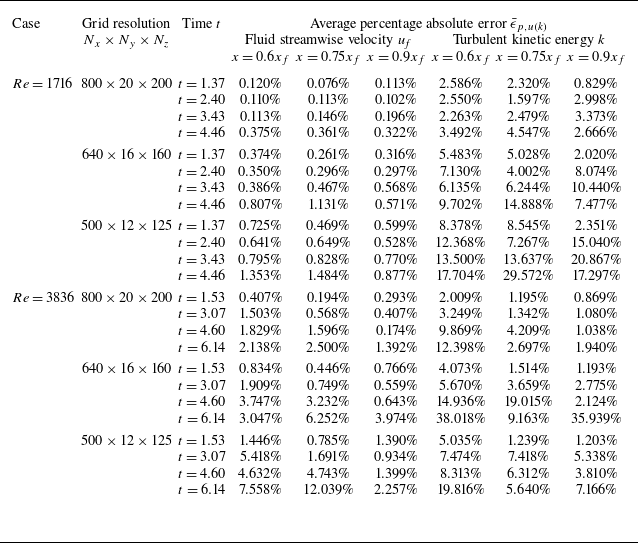
. In order to quantitatively analyse the impact of grid resolution on the calculation results, we use the results obtained by the finest grid calculation as a reference and evaluated the average percentage absolute error
 $\bar {\epsilon }_{p,u(k)}$
of the profiles for different cases, at different times and at different locations. Taking the fluid streamwise velocity
 $u_{\!f}$
as an example,
 $\bar {\epsilon }_{p,u}$
is calculated as
 \begin{equation} \epsilon _{p,u} = \frac {1}{\max \big(u_{\!f}^{R}\big) - \min \big(u_{\!f}^{R}\big)} \frac {\sum \limits _{i = 1}^{N_{sam}} \left |u_{\!f}^C(z_i) - u_{\!f}^{R}(z_i)\right |}{N_{sam}} \times 100\,\%, \end{equation}
where
 $N_{sam}$
is the number of sampling points in the profile,
 $u_{\!f}^C(z_i)$
is the fluid streamwise velocity with coarser resolution at
 $z_i$
and
 $u_{\!f}^R(z_i)$
is the fluid streamwise velocity with finest (reference) resolution at
 $z_i$
. The average percentage absolute errors
 $\bar {\epsilon }_{p,u(k)}$
are listed in table 2.
Average percentage absolute error
 $\bar {\epsilon }_{p,u(k)}$
for different grid resolutions.

As shown in figure 2, the profiles basically align across different grid resolutions, regardless of whether the Reynolds number is high or low, indicating that the grid fineness is sufficient to achieve convergent results. Quantitatively, the grid with the resolution of
 $N_x \times N_y \times N_z = 800 \times 20 \times 200$
exhibits the lowest average percentage absolute errors, generally below
 $10\,\%$
(see table 2). To strike a balance between calculation efficiency and accuracy, grid resolutions of
 $N_x \times N_y \times N_z = 800 \times 20 \times 200$
,
 $N_x \times N_y \times N_z = 800 \times 40 \times 200$
and
 $N_x \times N_y \times N_z = 800 \times 80 \times 200$
are respectively used for the computation of cases
 $1-5$
, 3a and 3b, as shown in table 1.
Additionally, in our current work, the ratio of the grid size
 $\text{d}_{x(yz)}$
to the Kolmogorov length scale
 $\eta$
is of the order of
 $O(10^{-1} \;{\sim}\; 10^0)$
. In all cases,
 ${d}_{x(yz)} / \eta \lt 1$
at most locations. Even at the highest Reynolds number (
 ${Re} = 3836$
), which represents the most challenging scenario, the maximum
 ${d}_{x(yz)} / \eta$
reaches only 1.2. This indicates that the grid resolution is sufficiently fine to resolve the turbulent cascade (Arthur & Fringer Reference Arthur and Fringer2014).
The lock-exchange TC exhibits obvious two-dimensional evolution characteristics as a whole, with two-dimensional and three-dimensional simulation results showing high similarity (Francisco, Espath & Silvestrini Reference Francisco, Espath and Silvestrini2017). The three-dimensional features of the TC interfacial KH billows depend on the flow Reynolds number
 ${\textit{Re}}$
and emerge primarily at the later stages of TC evolution. This study focuses on the two-dimensional (longitudinal and vertical) evolution characteristics of the TC and its interfacial KH billows at moderate Reynolds numbers. Consequently, spanwise-averaged quantities are primarily used to analyse the evolution mechanism. Furthermore, volume averaging is applied to the fluid and particle physical quantities within the selected volume
 $\mathcal{A}$
, i.e.
 \begin{align}&\qquad\qquad\qquad\quad \langle \mathscr{Q}^f \rangle _{\mathcal{A}} = \frac {\int \alpha _f \mathscr{Q}^f \textrm{d} \mathcal{A}}{\int \alpha _f \textrm{d} \mathcal{A}}, \end{align}
 \begin{align}& \left\langle \mathscr{Q}^p \right\rangle _{\mathcal{A}} = \frac {1}{N_{p,\mathcal{A}}} \sum \limits _{i = 1}^{N_{p,\mathcal{A}}} \mathscr{Q}^p_i \quad\textrm{for particles whose}\; \boldsymbol{x}_{p,i} \in \mathcal{A}, \end{align}
where
 $\mathscr{Q}^f$
and
 $\mathscr{Q}^p_i$
represent the fluid variables and the variables of particle
 $i$
before volume averaging, respectively;
 $\langle \mathscr{Q}^f\rangle _{\mathcal{A}}$
and
 $\langle \mathscr{Q}^p\rangle _{\mathcal{A}}$
denote the averaged variables over a selected volume
 $\mathcal{A}$
for fluid and particle phases, respectively;
 $N_{p,\mathcal{A}}$
is the number of particles in volume
 $\mathcal{A}$
; and
 $\boldsymbol{x}_{p,i} = (x_{p,i},y_{p,i},z_{p,i})$
denotes the spatial position of particle
 $i$
.
3. Revisiting TC regimes at moderate Reynolds numbers
3.1. Spatial distribution of particle and fluid velocity
Time evolution of fluid velocity field and particle motion. Results are shown for (
 $a$
)
 $t = 0.61$
, (
 $b$
)
 $t = 1.21$
, (
 $c$
)
 $t = 1.52$
, (
 $d$
)
 $t = 1.82$
, (
 $e$
)
 $t = 2.42$
, (
 $f$
)
 $t = 3.03$
, (
 $g$
)
 $t = 4.24$
, (
 $h$
)
 $t = 5.45$
, (
 $i$
)
 $t = 6.67$
and (
 $j$
)
 $t = 7.88$
. The slice indicates the spatial distribution of the spanwise-averaged fluid streamwise velocity
 $u_{\!f}$
with the grey lines representing the streamlines of the spanwise-averaged fluid velocity
 $\boldsymbol{u}_f$
. Particles are coloured with particle streamwise velocity
 $u_{{\kern-1pt}p}$
.

This section discusses the result of case 3 (
 ${Re}=3030$
) as an example. Figure 3 illustrates the time evolution of the fluid velocity field and particle behaviour. It can be seen from the figure that under the dominance of particle gravity, the particle–fluid mixture gradually collapses and evolves into a TC downstream. This development process aligns with findings from previous studies (Cantero et al. Reference Cantero, Balachandar and García2008; Espath et al. Reference Espath, Pinto, Laizet and Silvestrini2015; Xie et al. Reference Xie, Hu, Zhu, Yu and Pähtz2023a
; Lu et al. Reference Lu, Liu, Xie, Sun, Yang and Guo2024). During the entire TC evolution, the interaction between particles and fluids causes the two phases to exhibit similar motion characteristics. At the very early stage of the collapse (figure 3
 $a$
), both the fluid and the particles in the turbidity front exhibit positive flow velocities. Due to the conservation of mass, the upper ambient fluid is pumped in the opposite direction into the lock (Cantero et al. Reference Cantero, Lee, Balachandar and Garcia2007), resulting in a counterclockwise flow in the ambient fluid region. This phenomenon explains why the fluid and particle streamwise velocities in the upper TC region are initially negative.
As the collapse progresses, the local positive particle and fluid streamwise velocities (
 $u_{{\kern-1pt}p}$
and
 $u_{\!f}$
) at some locations near the interface within the TC region increase, as shown in figure 3(
 $b$
–
 $d$
). This is accompanied by an increase in the negative streamwise velocity of the ambient fluid on the upper side of the TC interface. It suggests that there is a local increase in shear between the TC and the ambient fluid. Consequently, a local flow trend emerges, moving away from the collapsing body, leading to undulations in the interface morphology and a loss of its initial smoothness. At
 $t = 2.42$
, a distinct KH billow composed of a series of anticlockwise KH vortex pairs appears as shear instability intensifies, as seen in figure 3(
 $e$
). This observation contrasts with the finding that KH billows do not form in TCs at low Reynolds numbers (Xie et al. Reference Xie, Hu, Pähtz, He and Cheng2022, Reference Xie, Hu, Zhu, Yu and Pähtz2023a
). It suggests that the larger flow Reynolds number
 ${\textit{Re}}$
, representing the ratio of inertial forces to viscous diffusion, promotes the development of interfacial instability of the lock-exchange TC (Ottolenghi et al. Reference Ottolenghi, Adduce, Inghilesi, Roman and Armenio2016). The KH vortex connects with the TC and entertains particles from it through the downstream side of the vortices. Some KH vortices merge and are eventually destroyed due to vortex–vortex interactions at
 $t = 3.03$
(figure 3
 $f$
). The primary reason is the intense shearing action brought about by the opposing vertical velocities of adjacent KH vortices (Cerretelli & Williamson Reference Cerretelli and Williamson2003). Simultaneously, as the current evolves, the reflected bore generated by the backflowing ambient fluid impacting the wall propagates forward (Shin, Dalziel & Linden Reference Shin, Dalziel and Linden2004) and eventually interacts with each KH vortex. It eventually rises upward under the obstruction of the downstream TC, as shown in figure 3(
 $g$
), generating a counterclockwise vortex structure that exists for a long time – this is consistent with Lu et al. (Reference Lu, Liu, Xie, Sun, Yang and Guo2024). In the vicinity of
 $x=2{\;{\sim}\;} 2.5$
, it induces a clockwise vortex by forcing the particles moving upward and forward, as depicted in figure 3(
 $h$
,
 $i$
), which was also reported in Cantero et al. (Reference Cantero, Lee, Balachandar and Garcia2007). Particles keep leaking out of the vortex in the centre of the simulation region in figure 3(
 $i$
,
 $j$
) because of the attenuation of vortex intensity caused by energy dissipation. Furthermore, an anticlockwise vortex is still generated close to the TC head (figure 3
 $g$
), where the reflected bore is not able to catch up, leading to particle ejection in figure 3(
 $h$
).
Time evolution of streamwise fluid–particle slip velocity
 $u_{\!f} - u_{{\kern-1pt}p}$
. Results are shown for (
 $a$
)
 $t = 0.61$
, (
 $b$
)
 $t = 1.21$
, (
 $c$
)
 $t = 1.52$
, (
 $d$
)
 $t = 1.82$
, (
 $e$
)
 $t = 2.42$
and (
 $f$
)
 $t = 3.03$
.

Figure 4 displays the spatial distribution of streamwise interphase slip velocity
 $u_{\!f}-u_{{\kern-1pt}p}$
, which directly reflects the direction of the drag force exerted by the fluid on the particles. Using the definition of the streamwise particle Reynolds number
 ${Re}_{p,x} = \rho _f {\textrm{d}}_p |u_{\!f} - u_{{\kern-1pt}p}|/{\mu} _f$
of the order of
 $O(10^{-4}$
), figure 4 also provides insight into the strength of the fluid–particle interaction in the streamwise direction. Streamwise slip velocity
 $u_{\!f} - u_{{\kern-1pt}p}$
, of less than
 $O(10^{-4})$
, reflects a weak deviation in streamwise velocity between the two phases, as the particle Stokes number
 $St$
is very small (
 $St \ll 1$
). Most areas in the TC body exhibit a low positive slip velocity, consistent with Eulerian–Eulerian results in Cantero et al. (Reference Cantero, Balachandar and García2008). In the early stages, a relatively significant positive slip velocity is observed near the left wall, while in the middle and later stages, it is primarily located near the upper interface of the middle and tail regions of the flow, which is linked to the downstream propagation of the reflected bore. The negative slip velocity is predominantly found near the upper interface, especially within the interfacial instability vortices, due to the shearing effect of the ambient fluid. This indicates that particles within these vortices experience substantial two-phase interactions.
Time evolution of fluid relative pressure
 $p'$
and vortical coherent structures. Results are shown for (
 $a$
)
 $t = 0.61$
, (
 $b$
)
 $t = 1.21$
, (
 $c$
)
 $t = 1.52$
, (
 $d$
)
 $t = 1.82$
, (
 $e$
)
 $t = 2.42$
and (
 $f$
)
 $t = 3.03$
. The slice shows the spatial distribution of the spanwise-averaged fluid relative pressure
 $p'$
. Translucent grey areas indicate TCs. Vortical coherent structures are captured by
 $Q$
-criterion (
 $Q = 5$
) that are marked in cyan.

Figure 5 depicts the spatial distribution of the fluid relative pressure
 $p'$
, which is defined as the difference between the fluid total pressure
 $p$
and the local theoretical hydrostatic pressure. During the early stages of the TC, particle sedimentation causes the lower fluids to exhibit a high relative pressure
 $p'$
, while the upper layer displays a low value (Si, Shi & Yu Reference Si, Shi and Yu2018). It also affects the relative pressure of the nearby ambient fluid, which exhibits comparable distribution features. As time goes by, regions of high relative pressure shift to the TC front and adjacent areas, as well as to the bottom of the initial fluid–particle collapse region. Affixed to the upper interface of the TC, the low relative pressure centre follows the TC in the longitudinal direction (Lee Reference Lee2019). In the early stages (figure 3
 $a$
–
 $e$
), the low-pressure centre’s relative pressure steadily falls, and in the latter stages (figure 3
 $e$
,
 $f$
), it gradually increases.
Figure 5 also depicts the coherent vortical structures captured by the
 $Q$
-criterion. The
 $Q$
value is given by the symmetric tensor and antisymmetric tensor of the fluid velocity gradient
 $\boldsymbol\nabla \boldsymbol{u}_f$
(Hunt, Wray & Moin Reference Hunt, Wray and Moin1988; da Silva & Pereira Reference De Silva, Fernando, Eaton and Hebert2008), i.e.
 \begin{equation} Q = \frac {1}{2}\left ( {\Omega _{ij}}{\Omega _{ij}} - {{S _{ij}}{S _{ij}}} \right ), \end{equation}
in which the symmetric tensor
 $\mathcal{S}_{ij}$
(strain rate tensor) and anti-symmetric tensor
 $\Omega _{ij}$
(rotation rate tensor) are determined by
 \begin{align}& \mathcal{S}_{ij} = \frac {1}{2} \left ( \frac {\partial u_{f,i}}{ \partial x_j} + \frac {\partial u_{f,j}}{\partial x_i} \right )\!, \end{align}
 \begin{align}& {\Omega _{ij}} = \frac {1}{2} \left ( \frac {\partial u_{f,i}}{\partial x_j} - \frac {\partial u_{f,j}}{\partial x_i} \right )\!. \end{align}
The figure illustrates that the coherent vortical structure mostly originates on the upper TC interface and that it significantly coincides with the low-pressure centre (Hunt et al. Reference Hunt, Wray and Moin1988; Jeong & Hussain Reference Jeong and Hussain1995), both of which are likely to be related to the KH vortices close to the interface. Thus, the KH vortex’s dynamic features can be well described by the coherent vortical structure’s attributes, such as particle count, vortex size and energy. This serves as the foundation for the analysis of the KH vortex dynamics in the text that follows.
Spatial distribution of particle vertical velocity divided by particle Stokes settling velocity
 $w_p / u_{\tau }$
at six selected times. Results are shown for (
 $a$
)
 $t = 0.6$
, (
 $b$
)
 $t = 1.8$
, (
 $c$
)
 $t = 2.4$
, (
 $d$
)
 $t = 3.0$
, (
 $e$
)
 $t = 3.6$
, (
 $f$
)
 $t = 4.2$
, (
 $g$
)
 $t = 5.5$
and (
 $h$
)
 $t = 6.7$
. The isosurface represents the vortical coherent structures captured at
 $Q=5$
with the colour indicating the spanwise fluid velocity
 $v_f$
.

The impact of the KH vortex on particle transport and settling behaviour is preliminarily addressed here. Figure 3 shows the impact of the KH vortex on horizontal particle transport, and the spatial distribution of the vertical particle velocity during the TC evolution is displayed in figure 6. As figure 3 illustrates, the interfacial KH vortices promote the streamwise transport of particles near the TC interface. In TCs with low Reynolds numbers (Xie et al. Reference Xie, Hu, Zhu, Yu and Pähtz2023a ), this vortex-related local particle transport enhancement is not visible. This can be explained in two ways: first, by the existence of the KH vortex, which prevents the ambient fluid and current from directly interacting, thereby lessening the ambient fluid’s shear on the TC interface; second, by the fluid force produced by the vortex structure acting as an accelerator.
The particle vertical velocity, shown in figure 6(
 $a$
), is initially generally higher than the particle Stokes velocity, i.e.
 $|w_p|\gt u_\tau$
, due to the influence of upper backflow. Subsequently, the particles on the upstream side of the vortices continue to settle at a speed greater than the Stokes velocity, while the particles near the downstream side of the vortex – especially those close to the head – tend to move upward due to the anticlockwise interfacial vortices (figure 6
 $c,\!d$
). The reflected wave is the primary cause of the extremely rapid particle settling within
 $x = 0 - 0.5$
in figure 6(
 $b$
–
 $d$
). In regions unaffected by the reflected wave and vortices, particles in the TC mostly settle at a speed of approximately
 $u_\tau$
.
The figure also presents a three-dimensional visualisation of the vortex coherent structures extracted by the
 $Q$
-criterion. In the early and middle stages, the vortex structures at the TC interface exhibit prominent two-dimensional characteristics. In the later stages (figure 6
 $f$
), the development of three-dimensional instability leads to the destruction of spanwise vortices and the breakdown of KH billows, consistent with the previous findings (Winant & Browand Reference Winant and Browand1974; Caulfield & Peltier Reference Caulfield and Peltier2000). Notably, in figure 6(
 $g$
,
 $h$
) a series of long coherent structures appear, connecting the TC with the resident vortex in the intermediate region, with opposite spanwise fluid velocities
 $v_f$
.
We investigate the relationship between the relative settling velocity of particles and the
 $Q$
value at the particle position in the flow, as depicted in figure 7. The relative particle settling velocity,
 $w_p-w_f$
, is defined as the difference between the particle vertical velocity and the fluid vertical velocity, which here is used to eliminate the influence of the TC background flow. As seen in the figure, there is a general positive correlation between the relative settling velocity
 $w_p-w_f$
and the
 $Q$
value, denoted as
 $w_p-w_f \;{\sim}\; Q$
. Specifically, negative
 $Q$
values are associated with an increase in particle settling velocity, while positive
 $Q$
values correlate with a decrease in settling velocity, which aligns with previous cognition (Maxey Reference Maxey1987; Tom & Bragg Reference Tom and Bragg2019). Maxey (Reference Maxey1987) explained this relationship by the preferential sweeping of settling inertial particles through negative
 $Q$
vortex regions under centrifugal force, which causes downward-moving vortices to intensify their downward motion. Furthermore, the relative settling velocity is mostly close to
 $u_\tau$
, as illustrated by
 $ (w_p-w_f ) / u_\tau \approx -1$
in figure 7.
Relationship between the vertical velocity of the particles after subtracting the fluid velocity (
 $w_p-w_f$
) and the
 $Q$
values at the particle positions for
 ${Re} = 3030$
. Results are shown for (
 $a$
)
 $t = 1.2$
, (
 $b$
)
 $t = 1.8$
, (
 $c$
)
 $t = 2.4$
, (
 $d$
)
 $t = 3.0$
, (
 $e$
)
 $t = 3.6$
and (
 $f$
)
 $t = 4.2$
. The black line shows the linear fitting result, and the fitting slope is shown in the figure.

Time evolution of the current front
 $x_f$
.

Spanwise-averaged TC profiles for different
 ${\textit{Re}}$
values at various times, which are distinguished by the particle volumetric fraction
 $\alpha _p = 10^{-5}$
. Results are shown for (
 $a$
)
 $t = 0.6$
, (
 $b$
)
 $t = 1.8$
, (
 $c$
)
 $t = 2.4$
, (
 $d$
)
 $t = 3.0$
, (
 $e$
)
 $t = 4.2$
and (
 $f$
)
 $t = 6.7$
.

3.2. Effect of Reynolds number on TC evolution
Figure 8 plots the time evolution of the front position,
 $x_f$
, of the TC under various
 ${\textit{Re}}$
conditions. The front position
 $x_f$
is defined as the distance between the farthest moving particle and the gate, i.e.
 $x_f = \max (x_{p,i}) - L_g$
, where
 $x_{p,i}$
is the particle position along the
 $x$
axis. As can be seen from the figure, the simulation results almost align with the previous results (Cantero et al. Reference Cantero, Lee, Balachandar and Garcia2007; Xie et al. Reference Xie, Zhu, Hu, Yu and Pan2023b
). However, the simulated TC front decelerates earlier, primarily due to the greater particle settling effect (Bonnecaze, Huppert & Lister Reference Bonnecaze, Huppert and Lister1993; Gladstone & Woods Reference Gladstone and Woods2000; Meiburg et al. Reference Meiburg, Radhakrishnan and Nasr-Azadani2015) and the aspect ratio of the initial fluid–particle column (Cantero et al. Reference Cantero, Lee, Balachandar and Garcia2007; Sun et al. Reference Sun, Zhang, Wang and Liu2020; Lu et al. Reference Lu, Liu, Xie, Sun, Yang and Guo2024). The time evolution of the front includes the initial collapse acceleration stage, the slumping stage characterised by a constant front velocity, and the later deceleration stage. The curves indicate that the constant velocity during the slumping stage is roughly 0.55, consistent with earlier simulation and experimental findings (Rottman & Simpson Reference Rottman and Simpson1983; Gladstone, Phillips & Sparks Reference Gladstone, Phillips and Sparks1998; Shin et al. Reference Shin, Dalziel and Linden2004; Steenhauer, Tokyay & Constantinescu Reference Steenhauer, Tokyay and Constantinescu2017). With increasing flow Reynolds number, the TC movement distance increases; additionally, the constant velocity of the slumping stage slightly increases, and its duration is extended. These findings are in line with the established understanding of how the Reynolds number influences TCs (Marino, Thomas & Linden Reference Marino, Thomas and Linden2005; Cantero et al. Reference Cantero, Lee, Balachandar and Garcia2007; Hu et al. Reference Hu, Tao, Li and He2020).
The TC profiles, captured by the particle volumetric fraction
 $\alpha _p = 10^{-5}$
, at six selected instants for various Reynolds numbers are displayed in figure 9. As can be observed in figure 9(
 $a$
), the initial collapse event of the fluid–particle mixture is independent of the Reynolds number during the early stages of the TC. Later on (figure 9
 $b$
–
 $f$
), however, the front position becomes positively correlated with the Reynolds number, which is consistent with the observations regarding the front position in figure 8. At this time, TCs with higher Reynolds numbers typically exhibit greater current thickness, demonstrating a higher ability of particle suspension. Furthermore, more KH vortices can be excited at the interface at high Reynolds numbers, aligning with the findings from simulations of KH billow development in a horizontally periodic domain (Smyth Reference Smyth2003; Fontane & Joly Reference Fontane and Joly2008). This corresponds to a decrease in wavelength of KH instability. Given their ability to promote particle transport and obstruct settling (figures 3 and 6), these KH vortices near the TC interface may be the cause of the higher transport levels of high Reynolds number TCs.
4. Assessment of effect of computational domain width on KH billows
Snapshots of flow field with different computational domain widths for case
 ${Re} = 3030$
. The vortex structure in the figure is defined by the
 $Q$
-criterion (
 $Q=5$
) and coloured by the fluid streamwise velocity
 $u_{\!f}$
. The light grey surface represents the TC profile. Results are shown for (
 $a$
,
 $b$
)
 $t = 1.8$
, (
 $c$
,
 $d$
)
 $t = 2.4$
, (
 $e$
,
 $f$
)
 $t = 3.0$
and (
 $g$
,
 $h$
)
 $t = 4.2$
. (
 $a$
,
 $c$
,
 $e$
,
 $g$
) Perspective view and (
 $b$
,
 $d$
,
 $f$
,
 $h$
) top view. Each set of subfigures presents simulations with domain widths of
 $L_y = 0.2$
,
 $L_y = 0.4$
and
 $L_y = 0.8$
, arranged from top to bottom.

Spanwise-averaged flow field at different domain widths. The slice indicates the spatial distribution of the spanwise-averaged fluid streamwise velocity
 $u_{\!f}$
. The vortex structure is defined by the
 $Q$
-criterion (
 $Q=5$
) in cyan. Black lines depict the envelope of the TC given by the particle volume fraction (
 $\alpha _p = 10^{-5}$
). Results are shown for (
 $a$
–
 $c$
)
 $t = 0.6$
, (
 $d$
–
 $f$
)
 $t = 1.8$
, (
 $g$
–
 $i$
)
 $t = 2.4$
, (
 $j$
–
 $l$
)
 $t = 3.0$
, (
 $m$
–
 $o$
)
 $t = 4.2$
and (
 $p$
–
 $r$
)
 $t = 6.7$
; (
 $a$
,
 $d$
,
 $g$
,
 $j$
,
 $m$
,
 $p$
)
 $L_y = 0.2$
, (
 $b$
,
 $e$
,
 $h$
,
 $k$
,
 $n$
,
 $q$
)
 $L_y = 0.4$
, and (
 $c$
,
 $f$
,
 $i$
,
 $l$
,
 $o$
,
 $r$
)
 $L_y = 0.8$
.

The differences between two-dimensional and three-dimensional features have been widely studied in TC simulations (Necker et al. Reference Necker, Härtel, Kleiser and Meiburg2002; Espath et al. Reference Espath, Pinto, Laizet and Silvestrini2014; Francisco et al. Reference Francisco, Espath and Silvestrini2017; He et al. Reference He, Zhao, Hu, Yu and Lin2018). It is generally believed that the main TC characteristics are two-dimensional, but the billows caused by interface instability is easily affected by secondary three-dimensional instability and has obvious three-dimensional characteristics (Mashayek & Peltier Reference Mashayek and Peltier2012a , Reference Mashayek and Peltierb ). Although our model is three-dimensional, the effect of computational domain width on interface instability is worth discussing.
Figure 10 shows the flow field visualisation at four selected moments with different computational domain widths (
 $L_y = 0.2- 0.8$
) for case
 ${Re} = 3030$
, and figure 11 shows the spanwise-averaged flow field. In our three-dimensional simulations, varying the width of the computational domain did not significantly affect the morphology or position of the interface vortex or the TC profiles. In the early stage of the TC (figure 10
 $a$
,
 $b$
and figure 11
 $a$
–
 $f$
), the simulation results from different domain widths are consistent, indicating the feasibility of using a narrower computational domain to simulate the early flow mainly controlled by the initial collapse (Necker et al. Reference Necker, Härtel, Kleiser and Meiburg2002; Espath et al. Reference Espath, Pinto, Laizet and Silvestrini2014). As the simulation progresses into the middle and late stages of the TC, the change in domain width has a limited impact on the interface dynamics. With increasing domain width, the morphology of the interface vortex is elongated along the streamwise direction (figure 11
 $d$
–
 $i$
). At the same time, the three-dimensional instabilities become more prominent, manifesting as unevenness in the interface vortex structure in the spanwise direction. This includes localised expansion and contraction, as well as bending of the structure (figure 10
 $d$
). Especially in the large-width simulations during the later stages, more elongated vortex structures resembling strips form near the interface. These structures are excited by pronounced vortices in the flow field and are connected to the TC body. Such differences due to computational domain width are expected to be larger at later times.
There is a consensus that three-dimensional instabilities delay the pairing and merging of the interface KH vortices (Mashayek & Peltier Reference Mashayek and Peltier2012a
,
Reference Mashayek and Peltierb
). In our study, three-dimensional structures can be observed even in the narrowest computational domain (
 $L_y=0.2$
). As the domain width increases, the streamwise stretching of the vortices weakens the vertical shear of fluid between them, which in turn impedes the vortex pairing process. Consequently, under conditions of larger domain widths, vortex pairing is slightly delayed.
In our work, there is a vortex structure that persists for longer periods in the flow field. The existence of this vortex in three-dimensional simulations remains a subject of debate. Some studies suggest that, due to the three-dimensional structures, three-dimensional simulations lack the energetic vortex phenomena observed in two-dimensional simulations (Necker et al. Reference Necker, Härtel, Kleiser and Meiburg2002; Espath et al. Reference Espath, Pinto, Laizet and Silvestrini2014). However, vortices of this nature have also been observed in some three-dimensional simulations (Gonzalez-Juez et al. Reference Gonzalez-Juez, Meiburg, Tokyay and Constantinescu2010; Nasr-Azadani & Meiburg Reference Nasr-Azadani and Meiburg2014; Lu et al. Reference Lu, Liu, Xie, Sun, Yang and Guo2024). Two potential factors may contribute to its presence in our simulations. First, the current computational domain width
 $L_y$
may not be sufficiently large. As
 $L_y$
increases from 0.2 to 0.8, the vortex tends to fragment gradually, and it may become absent at larger computational domain widths. Second, the particle settling effect could play a role. This vortex primarily forms in the middle and rear sections of the TC, where the flow’s forward momentum is insufficient to transport particles forward. The interaction between the flow structure induced by particle settling and the TC flow, along with the wall-reflected bore, could give rise to this pronounced vortex. This issue warrants further investigation in future studies.
Overall, the influence of the computational domain width on three-dimensional simulations is limited and does not lead to qualitative changes in TC dynamics within the range of
 $L_y = 0.2-0.8$
. A computational domain width of
 $L_y = 0.2$
is sufficient to capture the essential TC dynamics and the key features of the instability process. Furthermore, the minimal differences in spanwise-averaged results across varying computational domain widths in figure 11 support the use of spanwise-averaged results within this range. These findings provide useful insights for future three-dimensional TC simulations.
5. Development of KH billows in TC evolution
5.1. Formation of KH billows
The instability of the TC upper interface is affected by velocity shear and density stratification. The stratification strength of the flow is characterised by the mixture density gradient in the numerator of (1.2), which can be carefully deduced to yield the following relationship:
 \begin{equation} \frac {\partial \rho _m}{\partial z} = \frac {\partial (\alpha _f \rho _f + \alpha _p \rho _p)}{\partial z} = \frac {\partial [(1-\alpha _p) \rho _f + \alpha _p \rho _p]}{\partial z} = (\rho _p - \rho _f)\frac {\partial \alpha _p}{\partial z}. \end{equation}
This implies that
 $\partial \rho _m / \partial z \varpropto \partial \alpha _p / \partial z$
, suggesting that the stratification can also be quantified by the particle volume fraction gradient
 $\partial \alpha _p / \partial z$
. Figure 12 displays the fluid streamwise velocity profile (
 $u_{\!f}$
) and particle concentration profile (
 $\alpha _p/\alpha _{p0}$
) of four cases at
 $t = 1.7$
, which is close to the critical moment of KH excitation. In terms of fluid velocity, the profiles for all cases are generally similar. The primary difference occurs in the region of strong shear near the upper interface of the TC flow – an increase in Reynolds number complicates the interface velocity profile at the upstream position (figure 12
 $a$
,
 $c$
). This may be a manifestation of greater susceptibility to instability. As for the particle concentration profiles, particles are suspended to a higher position at larger Reynolds numbers. Notably, the velocity profile does not exactly coincide with the particle concentration profile, especially at low Reynolds numbers (
 ${Re}=1716$
), as shown by the red line in figure 12(
 $g$
,
 $h$
). The offset between the velocity and particle concentration interfaces is indicative of asymmetric KH instability, which is related to the hybrid mode of symmetric KH instability and Holmboe instability (Olsthoorn et al. Reference Olsthoorn, Kaminski and Robb2023; Yang et al. Reference Yang, Timmermans and Lawrence2024a
). Additionally, this offset may be related to the different dominant wavenumber and amplitude caused by different boundary conditions above and below the TC interface at different Reynolds numbers (Carpenter et al. Reference Carpenter, Tedford, Rahmani and Lawrence2010), which in turn lead to different interface instability modes. This instability ejects particles away from the TC upper interface, resulting in a sharp interface (Yang et al. Reference Yang, Timmermans and Lawrence2024a
), as demonstrated by the profile at
 ${Re}=1716$
in figure 9(
 $f$
). Figure 13 shows the interfacial shear Reynolds number
 ${Re}_I$
of the velocity profile at different streamwise positions at
 $t=1.7$
. In a TC event,
 ${Re}_I$
is generally larger at the TC front, as it is the first to experience ambient fluid shear. As the TC flow Reynolds number
 ${\textit{Re}}$
increases, the interfacial shear Reynolds number
 ${Re}_I$
also increases, with a scaling relationship of
 ${Re}_I\;{\sim}\; {Re}^{1.25}$
typically holding between the two.
Profiles of spanwise-averaged fluid streamwise velocity and particle volume fraction for varying
 ${\textit{Re}}$
cases at
 $t = 1.7$
. (
 $a$
,
 $c$
,
 $e$
,
 $g$
) Fluid streamwise velocity
 $u_{\!f}$
and (
 $b$
,
 $d$
,
 $f$
,
 $h$
) particle volume fraction that is divided by the initial particle volume fraction
 $\alpha _p / \alpha _{p0}$
. Results are shown for (
 $a$
,
 $b$
)
 $x = 0.44$
, (
 $c$
,
 $d$
)
 $x = 0.59$
, (
 $e$
,
 $f$
)
 $x = 0.73$
and (
 $g$
,
 $h$
)
 $x = 1.20$
.

Interfacial shear Reynolds number
 ${Re}_I$
versus flow Reynolds number
 ${\textit{Re}}$
at various positions at
 $t = 1.7$
.

Spatial distribution of gradient Richardson number
 $Ri_g$
of case
 ${Re} = 3836$
at (
 $a$
)
 $t = 1.7$
and (
 $b$
)
 $t = 3.7$
. Black lines depict the envelope of the TC given by the particle volume fraction (
 $\alpha _p = 10^{-5}$
). The high-
 $Ri_g$
region beneath the low-
 $Ri_g$
region, where the KH instability is excited, is outlined by a red dashed ellipse. The gradient Richardson number profiles at the selected vortex excitation positions are displayed in the inset in panel (
 $a$
) and the two right insets in panel (
 $b$
). The left inset in panel (
 $b$
) shows the statistical results of the gradient Richardson numbers
 $Ri_g$
near the TC interface where the interfacial vortices are excited at different
 ${\textit{Re}}$
values.

Time evolution of (
 $a$
) interfacially averaged fluid streamwise velocity gradient
 $\langle -\textrm{d} u_{\!f} / \textrm{d} z\rangle _{\textit{IF}}$
, (
 $b$
) interfacially averaged particle volume fraction gradient
 $\langle -\textrm{d} \alpha _p / \textrm{d} z\rangle _{\textit{IF}}$
, and (
 $c$
) interfacially averaged gradient Richardson number
 $\langle Ri_g\rangle _{\textit{IF}}$
.

Figure 14 displays the spatial distribution of the gradient Richardson number
 $Ri_g$
, defined by (1.2), at two moments (
 $t=1.7$
and
 $3.7$
) for the
 ${Re}=3836$
case. The stratification effect is dominant in the green areas where
 $Ri_g \gt 1$
, whereas the shear effect is dominant in the pink areas where
 $0\lt Ri_g\lt 1$
. The TC front, the region where the TC body borders the bottom wall, and the area where the TC interacts with the ambient fluid are the three main locations where shear dominance occurs. As shown in the insets of figure 14, the gradient Richardson number (
 $Ri_g$
) near the interface, particularly at the location of the KH vortex initiation, is less than 1, with most values falling in the region of
 $Ri_g \lt 1/4$
. This observation aligns with previous studies (Turner Reference Turner1986; Kneller et al. Reference Kneller, Nasr-Azadani, Radhakrishnan and Meiburg2016). Notably, this threshold is less stringent than the critical value of
 $Ri_g = 1/4$
, a `rule of thumb’, which has been discussed by many studies (Harang et al. Reference Harang, Thual, Brancher and Bonometti2014; Howland, Taylor & Caulfield Reference Howland, Taylor and Caulfield2018; Parker, Caulfield & Kerswell Reference Parker, Caulfield and Kerswell2019). The offset between the particle concentration interface and the velocity interface induces asymmetry, which drives the upward extension of KH instability (Yang et al. Reference Yang, Timmermans and Lawrence2024a
) and contributes to the reduction of
 $Ri_g$
. Additionally, the unsteadiness of TC flow (Caulfield Reference Caulfield2021) and the reduction in velocity gradients due to particle settling dynamics (Kneller et al. Reference Kneller, Nasr-Azadani, Radhakrishnan and Meiburg2016) may enable KH instability to occur at slightly higher
 $Ri_g$
values. The critical threshold of
 $Ri_g$
in TCs thus remains a subject of ongoing investigation. Here
 $Ri_g$
values below the critical threshold do not always result in interface instability. In other words, a
 $Ri_g$
value below the threshold is only a prerequisite that must be met in order for the KH vortex to start.
It is worth mentioning that in the early stages of the lock-exchange TC, such as at
 $t=1.21$
in figure 3(
 $b$
), slight signs of instability can be observed, which is primarily attributed to the vertical shear term (
 $\partial w_f / \partial x$
) at the interface of the collapsing fluid–particle column. During this phase, the Miles–Howard criterion, typically used to predict the stability of stratified shear flows, may no longer be valid. Subsequently, the particle column collapse progresses rapidly into the horizontal development stage (see
 $t = 1.82$
in figure 3
 $d$
). At this stage, most interface vortex structures are governed by the horizontal shear term (
 $\partial u_{\!f}/\partial z$
), with the exception of vortices near the sidewalls that remain strongly influenced by reflected bore. The empirical
 $Ri_g$
criterion can then be used to analyse these vortex structures.
The gradient Richardson number profile does not exhibit a discernible pattern of increase or decrease. Interestingly, though, a stratification-dominated region dyed with dark green (
 $Ri_g \gt 10^2$
) always lies directly below the
 $Ri_g\lt 1$
region where the interfacial vortices are excited. Because of the strong stratification effect, the cost of vertical momentum transfer and mixing between the upper and lower fluids increases to a certain extent (Noh & Fernando Reference Noh and Fernando1995; Caulfield Reference Caulfield2021). This creates a scenario where the lower fluids act as a barrier, preventing the upper fluids from penetrating downward, thereby, in a sense fostering an environment conducive to the upward excitation of instabilities.
To further investigate the relationship between interface instability and Reynolds number, we select a region extending 0.025 in both the upward and downward directions (i.e. a vertical thickness of 0.05 in dimensionless units) relative to the three-dimensional upper interface of the TC, and the physical quantities in this region are then averaged to obtain the interfacially averaged quantities
 $\langle \boldsymbol\cdot \rangle _{\textit{IF}}$
. The time evolution of the interfacially averaged fluid streamwise velocity gradient
 $\langle -\textrm{d} u_{\!f} / \textrm{d} z\rangle _{\textit{IF}}$
, particle volume fraction gradient
 $\langle -\textrm{d} \alpha _p / \textrm{d} z\rangle _{\textit{IF}}$
and gradient Richardson number
 $\langle Ri_g\rangle _{\textit{IF}}$
is plotted in figure 15. As can be observed in figure 15(
 $b$
) and in figure 12, an increase in Reynolds number slightly increases the interface particle volume fraction gradient
 $\langle -\textrm{d} \alpha _p / \textrm{d} z\rangle _{\textit{IF}}$
, with the effect remaining within one order of magnitude. Due to the greater TC height at large
 ${\textit{Re}}$
, a larger fluid velocity gradient is observed in the interface (figure 12). The positive contribution of the increasing Reynolds number to
 $\langle -\textrm{d} u_{\!f} / \textrm{d} z\rangle _{\textit{IF}}$
is more than an order of magnitude as illustrated in figure 15(
 $a$
), exhibiting greater than its effect on
 $\langle -\textrm{d} \alpha _p / \textrm{d} z\rangle _{\textit{IF}}$
. Accordingly, this produces a smaller gradient Richardson number at a larger Reynolds number, as reported in previous studies (Salehipour et al. Reference Salehipour, Peltier, Whalen and MacKinnon2016b
; Caulfield Reference Caulfield2021), which means that the TC interface is more susceptible to shear instability. This explains why higher Reynolds number TCs develop larger and more numerous KH billows, as shown in figure 9.
Spatial distribution of forces acting on the particles of case
 ${Re} = 3030$
at
 $t = 1.7$
. (
 $a$
,
 $b$
) Total forces
 $\boldsymbol{F}^T$
, (
 $c$
,
 $d$
) effective drag force
 $\boldsymbol{F}^{Ed}$
, (
 $e$
,
 $f$
) lift force
 $\boldsymbol{F}^l$
, (
 $g$
,
 $h$
) added mass force
 $\boldsymbol{F}^{\textit{add}}$
, (
 $i$
,
 $j$
) pressure gradient force
 $\boldsymbol{F}^{q}$
and (
 $k$
,
 $l$
) viscous force
 $\boldsymbol{F}^{\boldsymbol\nabla \boldsymbol\cdot \boldsymbol{\tau }}$
. (
 $a$
,
 $c$
,
 $e$
,
 $g$
,
 $i$
,
 $k$
) Streamwise component
 $\boldsymbol{F}_x$
and (
 $b$
,
 $d$
,
 $f$
,
 $h$
,
 $j$
,
 $l$
) vertical component
 $\boldsymbol{F}_z$
.

Spatial distribution of forces acting on the interfacial particles of various cases at
 $t = 1.7$
. (
 $a$
,
 $b$
) Total forces
 $\boldsymbol{F}^T$
, (
 $c$
,
 $d$
) effective drag force
 $\boldsymbol{F}^{Ed}$
, (
 $e$
,
 $f$
) lift force
 $\boldsymbol{F}^l$
, (
 $g$
,
 $h$
) added mass force
 $\boldsymbol{F}^{\textit{add}}$
and (
 $i$
,
 $j$
) pressure gradient force
 $\boldsymbol{F}^{q}$
. (
 $a$
,
 $c$
,
 $e$
,
 $g$
,
 $i$
) Streamwise component
 $\boldsymbol{F}_x$
and (
 $b$
,
 $d$
,
 $f$
,
 $h$
,
 $j$
) vertical component
 $\boldsymbol{F}_z$
. The scatter represents the forces on the interfacial particles (within 0.05 dimensionless thickness from the TC interface), and the curve represents the spatial variation of average force on the interfacial particles
 $\langle \boldsymbol{F} \rangle _{\textit{IF}}$
.

Figure 16 depicts the spatial distribution of the forces acting on the particles in the vicinity of the KH excitation moment (
 $t=1.7$
) at
 ${Re} = 3030$
. These forces include the total force on the particles
 $\boldsymbol{F}^T$
, the effective drag force
 $\boldsymbol{F}^{Ed}$
(the sum of the drag force and the effective gravity), the lift force
 $\boldsymbol{F}^l$
, the added mass force
 $\boldsymbol{F}^{\textit{add}}$
, the pressure gradient force
 $\boldsymbol{F}^{q}$
and the viscous force
 $\boldsymbol{F}^{\boldsymbol\nabla \boldsymbol\cdot \boldsymbol{\tau }}$
. Given the low particle volume fraction of the TCs in this study (
 $O(10^{-4} \;{\sim}\; 10^{-3})$
) and accordingly the low particle collision frequency, the contact force is negligible on average. Thus, the contact force is not shown in the figure.
The components of each force in figure 16 are all smaller than the predominant vertical effective gravity of the suspended particles driving the TC process, which is associated with the dilution regime associated at low volume fraction (Balachandar & Eaton Reference Balachandar and Eaton2010). Nevertheless, despite its small magnitude, this interaction force plays a subtle yet significant role in the evolution of TCs through complex interphase interactions (Xie et al. Reference Xie, Hu, Pähtz, He and Cheng2022). With regard to the total force acting on the particles of KH vortices, it is observed that in the streamwise direction (figure 16
 $a$
) the particles in the front part of the vortex experience a negative total force, whereas the particles in the rear undergo a positive total force; in the vertical direction (figure 16
 $b$
) the particles in the upper and lower regions experience, respectively, a negative total force and a positive total force. This suggests that the fluid force applied by the KH vortex on the particles is convergent, which is in line with Lee (Reference Lee2019). This effect facilitates the particle accumulation within the vortex. Conversely, the particles’ response to the fluid is divergent, meaning that they will, in a way, impede the formation of the KH structure. The forces on particles in the TC are also affected by the KH vortices. The majority of particles, with the exception of those in the head region, receive positive
 $\boldsymbol{F}^T_x$
and
 $\boldsymbol{F}^T_z$
, which facilitate streamwise transport and vertical suspension of particles, respectively. This explains the spatial distribution of particle velocity shown in figures 3 and 6.
The spatial distribution of the total force on particles near the KH billows exhibits significant similarity to the spatial distribution of the added mass force (figure 16
 $g$
,
 $h$
) and the pressure gradient force (figure 16
 $i$
,
 $j$
). Given that the fluid acceleration and particle acceleration are relatively synchronised when
 $St \ll 1$
, the strong correlation observed between the total force and the added mass force makes sense. The pressure gradient force is primarily closely related to the spatial distribution of pressure in figure 5. It is evident that the low-pressure centre formed by the interfacial vortex plays a crucial role in entraining particles.
Furthermore, as figure 16(
 $c$
) illustrates, shear from the ambient fluids causes particles close to the upper TC interface, including those in KH billows, to experience a negative streamwise effective drag force. There is a negative vertical effective drag on average (figure 16
 $d$
) because the vertical drag is insufficient to resist the particle gravity as they settle. Positive streamwise lift force and positive vertical lift force are produced on the interfacial particles by the negative
 $u_{\!f}-u_{{\kern-1pt}p}$
and positive
 $w_f-w_p$
under the control of the anticlockwise flow near the interface, which is represented as positive vorticity
 $\Omega _{xz}$
. It validates the lift’s beneficial contribution to particle suspension and transport in TCs, as concluded by Xie et al. (Reference Xie, Hu, Pähtz, He and Cheng2022), especially to rolling up the interfacial particles. On average, the fluid’s viscous force on the particles inhibits their streamwise movement at the TC interface but helps to their suspension.
Akin to the distribution of the added mass force and the pressure gradient force in figure 16(
 $g$
–
 $j$
), the fluid force on the particles away from the TC interface is also evidently influenced by the KH billows. Due to the large-scale start-up vortex created by rolling up the edges of the vorticity sheet, the particles in the head are subject to a negative total streamwise force. It is explained by the dominance of the added mass force and the pressure gradient force. The back particles experience a positive streamwise force from the fluids.
Figure 17 shows the various forces acting on the TC interface particles at different flow Reynolds numbers, and plots the distribution of the average forces applied to the particles along the
 $x$
direction. The viscous force
 $\boldsymbol{F}^{\boldsymbol\nabla \boldsymbol\cdot \boldsymbol{\tau }}$
is not depicted in the figure since it is of a comparatively negligible order as compared with other predominant forces (figure 16). As can be observed, with the Reynolds number of the TC increasing, the total force and the component forces also increase, though to different degrees. In particular, the lift force, added mass force and pressure gradient force – crucial for particles rolling up – increase with Reynolds number, facilitating the rolling up of interface particles in instability billows. This explains why, as the Reynolds number rises, the behaviour of particles rolling up becomes more pronounced as shown in figure 9.
5.2. Evolution mechanism of KH billows
(
 $a$
) Relative particle volumetric fraction
 $\langle \alpha _{p} \rangle _V / \alpha _{p0}$
and (
 $b$
) average particle Reynolds number
 $\langle {Re}_p \rangle _V$
in the typical KH vortices of case
 ${Re} = 3030$
. Vortices A–D are shown in figure 5.

Spatial distribution of finite-time Lyapunov exponent (FTLE) when
 ${Re} = 3030$
at six instants. Results are shown for (
 $a$
)
 $t = 0.61$
, (
 $b$
)
 $t = 1.21$
, (
 $c$
)
 $t = 1.52$
, (
 $d$
)
 $t = 1.82$
, (
 $e$
)
 $t = 2.42$
and (
 $f$
)
 $t = 3.03$
. Vortical coherent structures are captured by
 $Q$
-criterion (
 $Q = 5$
) that are marked in cyan.

For the KH billow evolution, we characterise the particle-carrying capacity and the strength of the fluid–particle interaction by using two physical quantities. They are the average particle concentration
 $\langle \alpha _{p0}\rangle _V/\alpha _{p0}$
and average particle Reynolds number
 $\langle {Re}_p \rangle _V$
of the vortex structures identified by
 $Q = 5$
. The particle Reynolds number
 ${Re}_p$
is determined by (2.15). The average particle volume fraction and average particle Reynolds number of four typical vortex structures in the case of
 ${Re}=3030$
(vortices A–D, marked in figure 5) are displayed over time in figure 18. Figure 18(
 $a$
) shows
 $\langle \alpha _{p0} \rangle _V/\alpha _{p0} \lt 1$
, suggesting that the average particle volume fraction of the vortices is always less than the initial particle concentration. The average particle volume fraction continues to drop as the interfacial vortex develops due to the expansion of the vortex structure (figure 5) and the rapid decline in the number of particles within it. The reflected bore is the cause of the increase in vortex A’s particle volume fraction at
 $t=2$
. With regard to the particle Reynolds number, figure 18(
 $b$
) reveals a progressive increase until the vortex merges or dissipates. It implies the enhancement of fluid–particle interactions as the vortices evolve.
The finite-time Lyapunov exponent (FTLE), which quantifies the local fluid stretching level, is often used to extract Lagrangian coherent structures (Lipinski & Mohseni Reference Lipinski and Mohseni2010; Balasuriya, Kalampattel & Ouellette Reference Balasuriya, Kalampattel and Ouellette2016; Rist, Weinschenk & Wenzel Reference Rist, Weinschenk and Wenzel2023). It helps in the assessment of the flow instability. Here, we compute the FTLE using the forward method in order to understand the evolution of interfacial KH billows in TCs. The spatial distribution of the FTLE at six chosen times during the TC process with
 ${Re}=3030$
is displayed in figure 19. Darker region in the image correspond to larger FTLE values where the fluid stretching is stronger.
A prominent feature of the large-scale FTLE structure with high stretching is its close correlation with the TC interface and the vortical coherent structures in the flow. The KH billows, which are part of the interface morphology, also exhibit a correlation with the FTLE structure. There is only a thin, sizable FTLE region close to the interface in the very early stage shown in figure 19(
 $a$
). The region progressively widens and the FTLE value dramatically rises as the current develops (figure 19
 $b$
), indicating an improvement in fluid stretching level. At
 $t = 1.52$
(figure 19
 $c$
), the large FTLE streak begins to become distorted, coinciding with the onset of interfacial particle flow instability (see figure 3
 $c$
). As the KH vortex is excited, the large FTLE streak evolves into a spatially continuous braided structure at
 $t=1.82$
in figure 19(
 $d$
). Three large FTLE streaks are visible in the typical vortex structure at
 $(x,z) = (0.6,0.6)$
in figure 19(
 $d$
). Two of these streaks originate from the downstream and upstream vortex structures, respectively, and they wrap around the middle largeFTLE streak up and down, which is located at the vortex centre. The particles are rolled up and firmly attached to the large FTLE streak from the downstream. The TC is connected to the ambient fluid by the low FTLE fluid in this braided structure, which destroys the initial spatially continuous large FTLE streak and facilitates the two fluids to mix. As the mixing progresses, the fluid near the TC interface exhibits a decreasing stretching level in figure 19(
 $e$
,
 $f$
), and some vortex structures are engulfed by other vortices.
The pairing and merging of KH vortices play a critical role in the development of interfacial instability, which significantly influences the mixing of the two fluids (TC and ambient fluid). This phenomenon represents the dominant two-dimensional instability in the evolution of KH billows (Yang et al. Reference Yang, Timmermans and Lawrence2024a
). In this context, the phase difference between the primary KH mode and the subharmonic mode, which governs vortex pairing (Dong et al. Reference Dong, Tedford, Rahmani and Lawrence2019; Liu et al. Reference Liu, Kaminski and Smyth2022), is influenced by the lock-exchange TC flow, particularly by the reflected bore that propagates downstream. We focus on the pairing process shown in figure 19(
 $e$
,
 $f$
), in which the three interfacial vortices pair and merge into two. This may correspond to the case of the phase of the subharmonic mode relative to the KH mode
 $\theta _{sub} = -\pi /2$
proposed in figure 1(
 $b$
) of Dong et al. (Reference Dong, Tedford, Rahmani and Lawrence2019), where the middle vortex is weakened and the vortices on both sides are strengthened.
Merging process of KH vortices during the TC evolution. Spatial distribution of (
 $a$
–
 $e$
) fluid rotation rate tensor
 $\Omega _{xz}$
, (
 $f$
–
 $j$
) fluid strain rate tensor
 $\mathcal{S}_{xz}$
, (
 $k$
–
 $o$
) FTLE, (
 $p$
–
 $t$
) particle streamwise velocity
 $u_{{\kern-1pt}p}$
and (
 $u$
–
 $y$
) total streamwise force acting on particles
 $\boldsymbol{F}^T_x$
. The first to fifth columns represent
 $t=2.42, 2.55, 2.67, 2.79$
and
 $3.03$
, respectively.

Here, we investigate this evolution mechanism from both the fluid and the particle phases. The spatial distribution of fluid rotation rate tensor
 $\Omega _{xz}$
, fluid strain rate tensor
 $\mathcal{S}_{xz}$
, FTLE, particle streamwise velocity
 $u_{{\kern-1pt}p}$
and total streamwise force acting on particles
 $\boldsymbol{F}^T_x$
during the vortex merging process of case
 ${Re}=3030$
are displayed in figure 20. Of note is the wall-reflected bore produced by the lock-exchange set-up. As shown in the figure, part of the flow structure formed by the development of the reflected bore gradually merges into vortex A, while the remainder travels beneath the KH billow. Although this process slightly affects the engulfment of vortex B, it does not qualitatively disrupt the merging mechanism. Therefore, the understanding of vortex merging presented here remains largely applicable to other similar scenarios.
Strong positive vorticity
 $\Omega _{xz}$
dominates the core of the KH vortices from the perspective of vorticity distribution (Parker et al. Reference Parker, Caulfield and Kerswell2019). Continuous vortex filaments develop on the front and rear sides of vortex B, connecting it with adjacent vortices (vortices C, D and A) (Parker et al. Reference Parker, Caulfield and Kerswell2019) before vortex B is engulfed and disappears. The fluid strain rate
 $\mathcal{S}_{xz}$
in the vortex filament area is very high as shown in figure 20(
 $f$
), particularly at the location where the vortex filaments are incredibly thin (Corcos & Sherman Reference Corcos and Sherman1976; Dong et al. Reference Dong, Tedford, Rahmani and Lawrence2019). Vortex B, as well as the front and rear vortices, are traversed by the braided structure of the large FTLE (figure 20
 $k$
,
 $l$
). The combined regime of strong vorticity and strong strain rate has a significant impact on the distribution of the FTLE. Vortex B flattens out as it shrinks due to the stretching force from the front and rear vortices. At the same time, the high fluid strain rate areas corresponding to the front and rear vortex filaments gradually merge in figure 20(
 $f$
–
 $i$
), and the braided structure of the large FTLE gradually becomes blurred. Finally, vortex B is eliminated. The regions of high FTLE, high strain rate
 $\mathcal{S}_{xz}$
and high positive vorticity
 $\Omega _{xz}$
gradually overlap during this merging process.
From the perspective of the particle movement, the root of vortex A moves forward more quickly due to the greater positive fluid streamwise force at the roots (figure 20
 $u$
,
 $v$
). As a result, vortex A in figure 20(
 $r$
,
 $w$
) catches up with the particles entrained in vortex B. When
 $t=2.55{\;{\sim}\;} 2.79$
, vortex A begins to progressively compress vortex B’s spatial position, leading to the eventual merging of vortex B into vortex A’s root. Regarding the different component forces illustrated in figure 31, the drag force, the added mass force and the pressure gradient force in the streamwise direction all work together to promote the merging process of this particle flow. This is largely affected by the strong pressure gradient between vortices, as shown in figure 5. Additionally, from figure 20(
 $f$
–
 $j$
,
 $p$
–
 $t$
), it can be observed that particles mainly accumulate or have a tendency to accumulate locally in regions with high strain rate
 $\mathcal{S}_{xz}$
rather than high vorticity
 $\Omega _{xz}$
, which accords with the general understandings of particle flows (Wang & Maxey Reference Wang and Maxey1993; Cantero et al. Reference Cantero, Balachandar and García2008).
6. Relation between KH vortices and particle motion
Herein, we explore the effects of vortex dynamics on particle transport and settling behaviour in detail. Particle transport can be quantitatively expressed in terms of particle volume flux,
 $Q^p_F$
, as
 \begin{align} Q^p_F (x) \equiv \left\langle \frac {1}{6}\pi {\textrm{d}}_p^3 u_{{\kern-1pt}p} \right\rangle _{\mathcal{G}} &= \frac {\pi {\textrm{d}}_p^3 }{6N_{p,\mathcal{G}}} \sum \limits _{i = 1}^{N_{p,\mathcal{G}}} u_{p,i} \quad \textrm{for particles whose}\notag\\ x_{p,i} \in \mathcal{G} &= \left(x-\frac {1}{2}{\textrm{d}}_x, x+\frac {1}{2}{\textrm{d}}_x\right], \end{align}
where
 $N_{p,\mathcal{G}}$
denotes the number of particles in the region
 $\mathcal{G}$
. Figure 21 illustrates the spatial distribution of the particle volume flux
 $Q_F^p$
and its streamwise gradient
 $\textrm{d}Q^p_F/\textrm{d}x$
at four selected instants for case
 ${Re}=3030$
. In figure 21(
 $a$
–
 $d$
) the particle flux
 $Q^p_F$
generally increases initially, then decreases along the streamwise direction. The reason why the maximum does not occur at the front is the strong resistance of the ambient fluid here, as seen in figure 3. Correspondingly, the particle flux gradient in figure 21(
 $e$
–
 $h$
) first increases to a positive value, then gradually decreases to a negative value, and finally becomes zero. The overall variation of
 $\textrm{d}Q^p_F/\textrm{d}x$
reflects the overall particle transport of the TC flow, while the local changes capture the influence of the local vortex structures on particle transport. It can be observed that, except for the vortices in the lock strongly affected by the reflected bore,
 $\textrm{d}Q^p_F/\textrm{d}x$
increase locally after passing through the interfacial vortices. This suggests that, although the upper section of the KH vortices generates negative particle flux, KH vortices generally promote the TC streamwise particle transport, especially for the particles in the lower part of the vortices.
Spatial distribution of (
 $a$
–
 $d$
) particle streamwise flux
 $Q^p_F$
and (
 $e$
–
 $h$
) its streamwise gradient
 $\textrm{d}Q^p_F/\textrm{d}x$
at various times for case
 ${Re} = 3030$
. Results are shown for (
 $a$
,
 $e$
)
 $t=1.8$
, (
 $b$
,
 $f$
)
 $t=2.1$
, (
 $c$
,
 $g$
)
 $t=2.4$
and (
 $d$
,
 $h$
)
 $t=3.0$
. The star symbol represents the spatial centre of the typical interfacial vortex structures captured by the
 $Q$
-criterion (
 $Q=5$
), and the shaded area indicates the spatial range of the corresponding vortices.

Time evolution of (
 $a$
) deposited particle mass
 $m_{depo}/\varSigma m_p$
and (
 $b$
) deposition rate
 $\textrm{d}(m_{depo}/\varSigma m_p ) /\textrm{d}t$
for different
 ${\textit{Re}}$
values.

Deposited particles are defined as stationary particles or particle clusters (
 $|\boldsymbol{u}_p|\lt 10^{-2}$
) in contact with the bottom wall. Figure 22 plots the time evolution of the total deposited particle number
 $m_{depo}/\varSigma m_p$
and the particle deposition rate
 $\textrm{d}(m_{depo}/\varSigma m_p) / \textrm{d}t$
, in which
 $m_{depo}$
is the deposited particle mass and
 $\varSigma m_p$
denotes the total mass of all the particles. It can be observed in figure 22(
 $a$
) that the amount of particle deposition progressively rises as the TC develops. In terms of particle deposition rate presented in figure 22(
 $b$
), there is a steady rise during the early stages of the TC. It is mainly due to the increase in the area covered by the TC (Cantero et al. Reference Cantero, Balachandar and García2008). Also, it is associated with the gradual development of flow created by the mass conservation-induced suction of ambient fluids into the lock. The rate of deposition peaks at approximately
 $t=3$
, after which it keeps declining. Such time evolution qualitatively agrees with the results in Cantero et al. (Reference Cantero, Balachandar and García2008).
Particle deposition generally proceeds more slowly as the Reynolds number increases as shown in figure 22(
 $a$
), which is consistent with Espath et al. (Reference Espath, Pinto, Laizet and Silvestrini2014). The early stage particle deposition rate in figure 22(
 $b$
) decreases with increasing Reynolds number
 ${\textit{Re}}$
. This is due to the fact that the backflow is weakened by the stronger KH vortices close to the TC interface as shown in figure 9. Additionally, the peak deposition rate is delayed by an increase in
 ${\textit{Re}}$
. The particle deposition rate decays more slowly in the middle and later stages (
 $t \gt 3$
) at the higher
 ${\textit{Re}}$
. With a low Reynolds number (
 ${Re}=1716$
), the particle deposition rate decays very quickly. This could be because there are insufficient interfacial vortices (figure 9), which prevent the sedimentation of particles. Remarkably, in the case of a high Reynolds number TC, there is a brief period of constant deposition rate at about
 $t=4$
and
 $t=6$
. This phenomenon is due to the strong influence of flow generated by the reflected bore, in conjunction with a few vortices, which exerts a significant impact on the deposited particles, leading to erosion in certain areas.
A small percentage of particles remain suspended and are not deposited in the later stages of the simulation, particularly at large Reynolds numbers (figure 22
 $a$
). This behaviour is primarily due to the presence of large-scale pronounced vortex structures in the flow field as shown in figure 9, which maintain the suspension of these particles (Necker et al. Reference Necker, Härtel, Kleiser and Meiburg2002).
Temporal and spatial distribution of the mass of deposited particles per unit area
 $\dot {m}_{depo}$
of case
 ${Re} = 3030$
.

The temporal and spatial variation of the mass of deposited particles per unit area
 $\dot {m}_{depo}$
is depicted in figure 23, and the variation of the deposited particle mass per unit area
 $\dot {m}_{depo}$
and the particle deposited rate per unit area
 $\textrm{d}\dot {m}_{depo} / \textrm{d}t$
at six selected locations (which is marked in figure 23) over time is shown in figure 24. In the lock region (
 $x\lt 0.5$
), the deposited particle mass per unit area
 $\dot {m}_{depo}$
first increases approximately linearly, corresponding to a roughly constant particle deposited rate
 $\textrm{d}\dot {m}_{depo} / \textrm{d}t$
. Deposition in this region is completed around
 $t=4.9$
, and then the deposited mass remains basically unchanged. The largest mass of deposited particles is found in the lock area (figures 23 and 24
 $a$
). In the region outside the lock, the particle deposition process begins upon the arrival of the TC front. The deposition rate here is essentially the same as it is in the lock in figure 24(
 $b$
), and
 $\dot {m}_{depo}$
increases approximately linearly as well at this time (figure 24
 $a$
). Notably, the deposited mass will still somewhat increase or decrease after the deposition is essentially finished, which is mainly due to the remained vortices transporting and eroding particles.
The spatial distribution of particle deposition
 $\dot {m}_{depo}$
shown in figures 23 and 24(
 $a$
) at various times is qualitatively consistent with TC simulation results with a low particle Stokes number (Gladstone et al. Reference Gladstone, Phillips and Sparks1998; De Rooij & Dalziel Reference De Rooij and Dalziel2001; Cantero et al. Reference Cantero, Balachandar and García2008). The deposited particle mass near
 $x = 1.8$
exhibits a local maximum. This is explained by a persistent vortex in the flow field in figure 3, which continues to release particles for deposition. Particle erosion (indicated by negative
 $\textrm{d}\dot {m}_{depo} / \textrm{d}t$
) can be observed near
 $x = 1$
at
 $t = 4$
and near
 $x = 1$
and
 $x = 2.5$
at
 $t = 6$
in figure 24(
 $b$
). It explains why the decay of the total particle deposition rate at
 $t = 4$
and
 $t = 6$
in figure 22(
 $b$
) is inhibited and the deposition rate remains relatively invariant.
Time evolution of (
 $a$
) the mass of deposited particles per unit area
 $\dot {m}_{depo}$
and (
 $b$
) particle deposited rate per unit area
 $\textrm{d}\dot {m}_{depo} / \textrm{d}t$
for case
 ${Re} = 3030$
at six selected positions.

Temporal and spatial distribution of bed shear stress
 $\tau _b$
of case
 ${Re} = 3030$
. Black line indicates the TC front position. Black bubbles represent some vortices close to the bottom wall in the TC process, and the size of the bubbles represents the size of the vortices.

It is widely acknowledged that there is a clear connection between bed shear stress
 $\tau _b$
and the deposition and erosion of particles, especially in the fields of geophysics and sedimentology (Fernandez Luque & Van Beek Reference Fernandez Luque and Van Beek1976; Pähtz et al. Reference Pähtz, Clark, Valyrakis and Durán2020). In order to comprehend how the vortex structure affects the particle deposition process, we investigate the relationship between
 $\tau _b$
and the vortex structures here. Figure 25 demonstrates the spatial and temporal distribution relationship of the bed shear stress. The bubble diagram in the figure depicts the vortices at a distance of less than 0.2 dimensionless length from the lowest point of the structure to the bottom boundary, with the bubble size indicating the size of the spanwise-averaged vortices identified using
 $Q$
-criterion (
 $Q=5$
). Strong bed shear stress is spatially distributed in a manner that is significantly correlated with the near-wall vortex structures (Cantero et al. Reference Cantero, Balachandar and García2008). Furthermore, the size of the vortices is generally positively associated with the bed shear stress at the corresponding location; for instance, the large-sized vortex structure at
 $x\approx 2.4$
and
 $t\approx 6$
generates great negative bed shear stress
 $\tau _b$
. The bed shear stress caused by the TC is predominantly positive, with occasional negative values that are mostly observed during
 $t=4{\;{\sim}\;} 7$
at about
 $x=2$
. This occurs because, while chasing the TC, the reflected bore merges with the interfacial vortices, causing the resulting flow to induce a clockwise vortex structure in the near-wall region, as shown in figure 3(
 $g$
–
 $j$
).
7. Energy conversion and its role in KH billows
7.1. Energy budget of TC evolution
We examine the influence of interfacial vortex structures on the evolution of TCs by analysing changes in energy components. First, we assess the total energy budget. The energy of the lock-exchange TC originates from the particle gravitational potential energy
 $E_p^p$
that is generated by particle settling (Parker, Fukushima & Pantin Reference Parker, Fukushima and Pantin1986; Necker et al. Reference Necker, Härtel, Kleiser and Meiburg2002; Nasr-Azadani & Meiburg Reference Nasr-Azadani and Meiburg2014; Zgheib, Bonometti & Balachandar Reference Zgheib, Bonometti and Balachandar2015). As particles settle, the fluid potential energy
 $E_p^f$
increases. The available potential energy,
 $E_{p,\textit{avail}}$
, is defined as the difference between the decrease in particle gravitational potential energy and the increase in fluid potential energy, i.e.
 $E_{p,\textit{avail}} = -\Delta E^p_p - \Delta E^f_p$
, in which the symbol
 $\Delta$
represents the variation in energy with respect to the initial time. Within the TC system, this available potential energy is converted into particle kinetic energy
 $E_k^p$
, fluid kinetic energy
 $E_k^f$
and dissipated energy
 $E_{\textit{Diss}}$
. This results in the following relationship (Xie et al. Reference Xie, Zhu, Hu, Yu and Pan2023b
):
 \begin{equation} \Delta {E_{\textit{Diss}}} = - \big[ {\Delta E_p^p + \Delta E_p^f + \Delta E_k^p + \Delta E_k^f} \big]. \end{equation}
Particle gravitational potential energy
 $E_p^p$
, particle kinetic energy
 $E_k^p$
, fluid potential energy
 $E_p^f$
and fluid kinetic energy
 $E_k^f$
are defined as follows in accordance with earlier research (Xie et al. Reference Xie, Hu, Pähtz, He and Cheng2022, Reference Xie, Zhu, Hu, Yu and Pan2023b
; Lu et al. Reference Lu, Liu, Xie, Sun, Yang and Guo2024; Yang et al. Reference Yang, Chen and Wang2024b
):
 \begin{align} E_p^p\left (t\right ) &= \sum \limits _{i=1}^{N_p} m_i \left |\boldsymbol{g}\right | z_{p,i}, \end{align}
 \begin{align} E_k^p\left (t\right ) &= \sum \limits _{i=1}^{N_p} \left ( \frac {1}{2} m_i |\boldsymbol{u}_{p,i}|^2 + \frac {1}{2} I |\boldsymbol{\omega }_{p,i}|^2 \right )\!, \end{align}
 \begin{align} E_p^f\left (t\right ) &= \int _{\mathcal{D}} \alpha _f \rho _f \left |\boldsymbol{g}\right | z \textrm{d} V, \end{align}
 \begin{align} E_k^f\left (t\right ) &= \int _{\mathcal{D}} \frac {1}{2} \alpha _f \rho _f |\boldsymbol{u}_f|^2 \textrm{d} V. \end{align}
Here
 $N_p$
denotes the particle number,
 $z_{p,i}$
is the elevation of the particle
 $i$
and
 $\mathcal{D}$
represents the whole simulation domain. Figure 26 illustrates how the various energy components alter as the TC evolves. With the initial particle gravitational potential energy
 $E^p_p(0)$
, the energy components in the figure are dimensionless.
Time evolution of the variation in energy components for varying cases. (
 $a$
) Particle gravitational potential energy
 $\Delta E^p_p$
, (
 $b$
) fluid potential energy
 $\Delta E^f_p$
, (
 $c$
) available potential energy
 $\Delta E_{p,\textit{avail}}$
, (
 $d$
) particle kinetic energy
 $\Delta E^p_k$
, (
 $e$
) fluid kinetic energy
 $\Delta E^f_k$
and (
 $f$
) dissipated energy
 $\Delta E_{\textit{Diss}}$
.

The figure illustrates that, as the currents evolve, the fluid potential energy
 $E_p^f$
, available potential energy
 $E_{p,\textit{avail}}$
and dissipated energy
 $E_{\textit{Diss}}$
all continue to rise, while the particle gravity potential energy
 $E_p^p$
consistently decreases. Particle gravity potential energy, fluid potential energy and available potential energy all progress (increase or decrease) at much higher rates at
 $t=0{\;{\sim}\;} 2$
than they do in the middle and later stages, as previously reported by other researchers (Necker et al. Reference Necker, Härtel, Kleiser and Meiburg2002, Reference Necker, Härtel, Kleiser and Meiburg2005; Ooi, Constantinescu & Weber Reference Ooi, Constantinescu and Weber2007; Nasr-Azadani & Meiburg Reference Nasr-Azadani and Meiburg2014). This rapid change is attributed to the initial collapse of the fluid–particle mixture. Both the fluid and particle kinetic energies (
 $E_k^f$
and
 $E_k^p$
) increase prior to
 $t=2$
and decrease thereafter. This pattern is due to the substantial supply of available potential energy during the early stage, which drives the kinetic energies, and the subsequent dissipation that reduces them in the later stage (Espath et al. Reference Espath, Pinto, Laizet and Silvestrini2015). The crucial time node,
 $t=2$
, marks when approximately
 $70\,\% -80\,\%$
of the initial particle potential energy
 $E^p_p(0)$
is transformed, yielding
 $E_{p,\textit{avail}}(t=2) = (\rho _p - \rho _f )/\rho _p |\Delta E^p_p (t=2) | \approx 0.3$
. Around
 $60\,\% -70\,\%$
of this available energy is crucial for the kinetic energies of particles and fluids, while the remaining
 $30\,\% -40\,\%$
of the energy is dissipated due to viscosity. This dissipation is slightly greater than that reported in previous studies (Espath et al. Reference Espath, Pinto, Laizet and Silvestrini2014; Nasr-Azadani & Meiburg Reference Nasr-Azadani and Meiburg2014), likely attributed to the increased terminal velocity of the particles,
 $u_\tau$
, in our TC simulations (Espath et al. Reference Espath, Pinto, Laizet and Silvestrini2015).
Both the potential energy change (
 $\Delta E_p^p$
in figure 26
 $a$
,
 $\Delta E_p^f$
in figure 26
 $b$
and
 $\Delta E_{p,\textit{avail}}$
in figure 26
 $c$
) and dissipated energy (figure 26
 $f$
) decrease with increasing Reynolds numbers
 ${\textit{Re}}$
. However, the kinetic energies of the particles and the fluid both rise (Espath et al. Reference Espath, Pinto, Laizet and Silvestrini2014), which is consistent with the observation that the TC front moves more quickly at higher Reynolds number in figure 8 (Cantero et al. Reference Cantero, Lee, Balachandar and Garcia2007). This may be related to the enhanced large-sized vortex structures and KH billows at higher Reynolds numbers (Necker et al. Reference Necker, Härtel, Kleiser and Meiburg2002; Espath et al. Reference Espath, Pinto, Laizet and Silvestrini2014; Francisco et al. Reference Francisco, Espath and Silvestrini2017). An intriguing implication is that a rise in Reynolds number will result in a decrease in the conversion ratio from the system’s available potential energy to dissipated energy, while increasing the conversion ratio to the kinetic energies. At the end of the simulation (
 $t=10$
), the potential energies (
 $E_p^p$
,
 $E_p^f$
and
 $E_{p,\textit{avail}}$
) are quickly converted and stabilise, and the particle kinetic energy
 $E_k^p$
approaches zero. However, the fluid kinetic energy
 $E_k^f$
is still in the process of being converted into dissipated energy and has not yet fully dissipated. This indicates the need for a longer simulation time to reach the final equilibrium state.
7.2. Energy dissipation route analysis
It is necessary to investigate how the dissipation process is weakened by an increase in Reynolds number and whether this effect is attained by varying the interfacial vortex structures. The dissipated energy is separated into three categories: dissipation from fluid viscosity
 $E_{\textit{Diss}}^f$
(called fluid dissipation), dissipation from particle collisions
 $E_{\textit{Diss}}^{p \leftrightarrow p}$
(called particle dissipation) and dissipation from fluid–particle interactions
 $E^{f \leftrightarrow p}_{\textit{Diss}}$
(called interaction dissipation). Thus, the following relationship is given:
 \begin{equation} E_{\textit{Diss}} = E_{\textit{Diss}}^f + E_{\textit{Diss}}^{p \leftrightarrow p} + E^{f \leftrightarrow p}_{\textit{Diss}}. \end{equation}
The dissipation resulting from particle collisions can be disregarded in this work, i.e.
 $E_{\textit{Diss}}^{p \leftrightarrow p} \approx 0$
, because the particle volume fraction
 $\alpha _{p0}$
of the TC is very low (
 $O(10^{-4} \;{\sim}\; 10^{-3})$
). Thus, (7.6) can be rewritten as
 \begin{equation} E_{\textit{Diss}} = E_{\textit{Diss}}^f + E^{f \leftrightarrow p}_{\textit{Diss}}. \end{equation}
The energy dissipated at time
 $t$
due to fluid viscosity,
 $E_{\textit{Diss}}^f$
, can be computed as
 \begin{equation} E_{\textit{Diss}}^f (t) = \int _0 ^t \int _{\mathcal{D}} \alpha _f \rho _f \epsilon \textrm{d} V {\textrm{d}}t, \end{equation}
where
 $\epsilon$
denotes the fluid dissipation rate, which is determined by (e.g. Rahmani et al. Reference Rahmani, Lawrence and Seymour2014a
; Vassilicos Reference Vassilicos2015; He et al. Reference He, Zhao, Zhu and Hu2019)
 \begin{equation} \epsilon = \nu _f \langle \mathcal{S}_{ij}\mathcal{S}_{ij} \rangle _{\mathcal{F\,V}}, \end{equation}
where
 $\langle \boldsymbol\cdot \rangle _{\mathcal{F\,V}}$
denotes an average over the fluid volume. Figure 27 shows the time evolution of the dissipated energy (
 $\Delta E_{\textit{Diss}}^f$
,
 $\Delta E_{\textit{Diss}}^V$
,
 $\Delta E_{\textit{Diss}}^{f \leftrightarrow p}$
), energy dissipation rate (
 $\textrm{d} E_{\textit{Diss}}^f/\textrm{d}t$
,
 $\textrm{d} E_{\textit{Diss}}^V/\textrm{d}t$
,
 $\textrm{d} E_{\textit{Diss}}^{f \leftrightarrow p}/\textrm{d}t$
) and the proportion of the dissipation component in the total dissipated energy (
 $\Delta E_{\textit{Diss}}^f / \Delta E_{\textit{Diss}}$
,
 $\Delta E_{\textit{Diss}}^V / \Delta E_{\textit{Diss}}$
,
 $\Delta E_{\textit{Diss}}^{f \leftrightarrow p} / \Delta E_{\textit{Diss}}$
) of different components, where
 $\Delta E_{\textit{Diss}}^V$
is the fluid dissipation of the vortical coherent region. The vortical coherent structures are captured by the
 $Q$
-criterion (
 $Q=5$
) as well, which essentially characterises the KH billows as seen in figure 5. The curves indicate that the dissipation process can be divided into two stages based on the dissipation rate,
 $t\lt 2$
and
 $t\gt 2$
, which shows the impact of collapse during the initial stage. The change rate of each dissipation component is rapidly increasing in the earlier phase, as illustrated in figure 27(
 $d$
–
 $f$
), and is generally decreasing in the subsequent stage. As a result, the early stage of dissipated energy in figure 27(
 $a$
–
 $c$
) exhibits a faster growth rate than in the later stage.
Process analysis of the energy dissipation. Time evolution of variation in (
 $a$
) fluid dissipation for the whole fluid domain
 $\Delta E^f_{\textit{Diss}}$
, (
 $b$
) fluid dissipation for the vortex domain
 $\Delta E^V_{\textit{Diss}}$
and (
 $c$
) interaction dissipation
 $\Delta E^{f \leftrightarrow p}_{\textit{Diss}}$
. Time evolution of the change rate of the above three dissipation components: (
 $d$
)
 $\textrm{d} E^f_{\textit{Diss}}/\textrm{d}t$
, (
 $e$
)
 $\textrm{d} E^V_{\textit{Diss}}/\textrm{d}t$
and (
 $f$
)
 $\textrm{d} E^{f \leftrightarrow p}_{\textit{Diss}}/\textrm{d}t$
. Time evolution of variation in the above dissipation components normalised by the total dissipation variation: (
 $g$
)
 $\Delta E^f_{\textit{Diss}} /\Delta E_{\textit{Diss}}$
, (
 $h$
)
 $\Delta E^V_{\textit{Diss}} /\Delta E_{\textit{Diss}}$
and (
 $i$
)
 $\Delta E^{f \leftrightarrow p}_{\textit{Diss}} /\Delta E_{\textit{Diss}}$
.

Generally speaking, an increase in Reynolds number at
 $t=0{\;{\sim}\;} 1$
reduces interaction dissipation (figure 27
 $f$
) but has a limited impact on fluid dissipation (figure 27
 $d$
,
 $e$
). The increase in
 ${\textit{Re}}$
at
 $t=1-4$
results in a decrease in the energy dissipation of each component. This has to do with the KH billows that form at the interface after
 $t=1$
. The increase in fluid dissipation at lower Reynolds numbers also may be attributed to the significant asymmetry between the fluid velocity and density profiles (Yang et al. Reference Yang, Timmermans and Lawrence2024a
), as shown in figure 12. The larger the Reynolds number, the stronger the interfacial vortex, which, acting as a transition zone, plays a role in reducing the shear between the ambient fluid and the TC. The curves for various
 ${\textit{Re}}$
cases in figure 27(
 $a$
–
 $c$
) have similar increments because, after
 $t = 4$
, the dissipation energy change rates become essentially independent of the Reynolds number (with the exception of
 ${Re} = 1716$
in figure 27
 $f$
). Because of the ongoing advancement of the reflected bore, the critical moment
 $t=4$
, where the Reynolds number shows a distinct effect, occurs slightly later than the moment
 $t=2$
, when the dissipation change rate reaches its maximum. After
 $t = 4$
, the interaction dissipation at low Reynolds number (
 ${Re} = 1716$
) drastically drops and almost reaches zero. The reason for this is that the current has essentially stopped moving at this time.
The fluid-particle interactions are responsible for a substantial portion of the energy dissipation in the TC process, as shown in figure 27(
 $g$
–
 $i$
). While the percentage of dissipation resulting from fluid–particle interaction in figure 27(
 $i$
) steadily declines, the percentage of dissipation due to the fluid viscosity in figure 27(
 $g$
) keeps rising. When
 $t\lt 4$
, the proportion of the dissipation brought on by fluid viscosity in the vortex structure (figure 27
 $h$
) initially rises and subsequently falls. Interestingly, after
 $t\gt 4$
, this proportion
 $\Delta E_{\textit{Diss}}^V / \Delta E_{\textit{Diss}}$
essentially stays constant and is independent of the Reynolds number, which is about 0.01.
(
 $a$
) Time evolution of average dissipation rates in the vortex region and in the fluid simulation domain
 $\langle \epsilon \rangle _V$
and
 $\langle \epsilon \rangle _f$
, and (
 $b$
) time evolution of the ratio between them
 $\langle \epsilon \rangle _V/ \langle \epsilon \rangle _f$
.

As illustrated in figure 28, we then go into great detail about the relationship between the average dissipation rate of the fluid region,
 $\langle \epsilon \rangle _f$
, and that of the vortex region,
 $\langle \epsilon \rangle _V$
. Both
 $\langle \epsilon \rangle _f$
and
 $\langle \epsilon \rangle _V$
rapidly increase in the early stages before progressively declining, essentially in time with the change in fluid kinetic energy in figure 26(
 $e$
). The peak of
 $\langle \epsilon \rangle _V$
occurs earlier than that of
 $\langle \epsilon \rangle _f$
. The value of
 $\langle \epsilon \rangle _V/\langle \epsilon \rangle _f$
in figure 28(
 $b$
), which always stays greater than 1, corresponds to the average dissipation rate in the vortex being always higher than the globally averaged fluid dissipation rate. Notably, its ratio exceeds 10 during the initial collapse stage of
 $t\lt 2$
, highlighting a significantly higher dissipation level for the fluids within the vortex structure. The ratio keeps going down as the TC evolves, mostly since
 $\langle \epsilon \rangle _V$
decays more quickly than
 $\langle \epsilon \rangle _f$
. The Reynolds number has a negligible effect on the ratio at
 $t\lt 2$
; however, at
 $t\gt 2$
, the ratio increases with increasing Reynolds number, which is indicative of a higher dissipation rate of vortex fluids. This observation further supports the notion that vortex structures are stronger at higher Reynolds numbers, consistent with the interpretation of the preceding figure 5.
Relationship between the average dissipation rate components of the interfacial vortices as the TC evolves: (
 $a$
)
 $\langle \epsilon _{\textit{NS}}\rangle _V$
vs
 $\langle \epsilon _{\textit{SD}}\rangle _V$
and (
 $b$
)
 $\langle \epsilon _{xx}\rangle _V$
vs
 $\langle \epsilon _{zz}\rangle _V$
. The colours of the symbols in panels (
 $a$
,
 $b$
) represent time
 $t$
. Snapshots of different stages of case
 ${Re} = 3030$
: (
 $c$
)
 $t = 1.21$
(stage I), (
 $d$
)
 $t = 1.33$
(the end of stage I), (
 $e$
)
 $t = 1.82$
(stage II), (
 $f$
)
 $t = 2.18$
(the end of stage II) and (
 $g$
)
 $t = 2.78$
(stage III). In panels (
 $c$
–
 $g$
) the slices show the spatial distribution of fluid vorticity
 $\Omega _{xz}$
, the black contour represents the TC profiles determined by the particle volume fraction
 $\alpha _p=10^{-5}$
, and the cyan contours are vortex structures captured by
 $Q$
-criterion (
 $Q=5$
).

Here we discuss the different components of average dissipation rate in the vortex structure. We decompose the dissipation rate
 $\epsilon$
into a part related to the normal strain
 $\epsilon _{\textit{NS}}$
and a remaining part related to the shear deformation
 $\epsilon _{\textit{SD}}$
:
 \begin{equation} \epsilon = \epsilon _{\textit{NS}} + \epsilon _{\textit{SD}}. \end{equation}
Given that the TCs in our work mainly exhibit noticeable two-dimensional characteristics before the onset of three-dimensional instability, the spanwise dissipation component at this stage is relatively negligible. Thus,
 $\epsilon _{\textit{NS}}$
and
 $\epsilon _{\textit{SD}}$
can be expressed by
 \begin{align} \epsilon _{\textit{NS}} &= \underbrace {\nu _f \langle \mathcal{S}_{xx}\mathcal{S}_{xx}\rangle _{\mathcal{F\,V}}}_{\epsilon _{xx}} + \underbrace { \nu _f \langle \mathcal{S}_{zz}\mathcal{S}_{zz}\rangle _{\mathcal{F\,V}}}_{\epsilon _{zz}}, \end{align}
 \begin{align} \epsilon _{\textit{SD}} &= \nu _f \left ( \langle \mathcal{S}_{xz}\mathcal{S}_{xz}\rangle _{\mathcal{F\,V}} + \langle \mathcal{S}_{zx}\mathcal{S}_{zx}\rangle _{\mathcal{F\,V}} \right ), \end{align}
where
 $\mathcal{S}_{xx}$
,
 $\mathcal{S}_{zz}$
,
 $\mathcal{S}_{xz}$
and
 $\mathcal{S}_{zx}$
can be calculated by (3.2). Figure 29 shows the relationship between the different average dissipation rate components of interfacial vortices and displays the fluid field snapshots at different stages. The dissipation process of the interfacial vortices can be divided into three stages in figure 29(
 $a$
) by using the approximate equalisation of
 $\langle \epsilon _{\textit{NS}}\rangle _V$
and
 $\langle \epsilon _{\textit{SD}}\rangle _V$
as a basis for stage division.
-
(i) Stage I: the dissipation rate from shear deformation
$\langle \epsilon _{\textit{SD}}\rangle _V$
is higher than that from normal strain
$\langle \epsilon _{\textit{NS}}\rangle _V$
, with
$\langle \epsilon _{\textit{SD}}\rangle _V$
gradually decreasing while
$\langle \epsilon _{\textit{NS}}\rangle _V$
increases. The relationship between the two dissipation rates can be described by(7.13)This indicates a mutual restriction between the dissipation intensity brought on by shear deformation and that brought on by normal strain. At this time, the vortex structures at the interface appear as slender strips (figure 29
\begin{equation} \frac {\textrm{d} \langle \epsilon _{\textit{NS}}\rangle _V}{\textrm{d} \langle \epsilon _{\textit{SD}}\rangle _V} \approx -1. \end{equation}
$c$
). This dissipation relationship persists until the two dissipation rates approach equilibrium, i.e.
$\langle \epsilon _{\textit{NS}}\rangle _V \approx \langle \epsilon _{\textit{SD}}\rangle _V$
, marking the end of the first stage.
-
(ii) Stage II: in this stage,
$\langle \epsilon _{\textit{SD}}\rangle _V$
is less than
$\langle \epsilon _{\textit{NS}}\rangle _V$
, and the interface vortex size keeps increasing. The difference between the major and minor axes of the elliptical vortex narrows and then expands (figure 29
$d$
–
$f$
), indicating that the vortex oblateness decreases and then increases. Here
$\langle \epsilon _{\textit{SD}}\rangle _V$
first decreases and then increases, exhibiting a positive correlation with vortex oblateness. In contrast,
$\langle \epsilon _{\textit{NS}}\rangle _V$
increases first and then decreases, which is negatively correlated with vortex oblateness. The time when stage II starts or ends (
$\langle \epsilon _{\textit{SD}}\rangle _V = \langle \epsilon _{\textit{NS}}\rangle _V$
) may be related to the oblateness of the vortex. At the end of this stage, both
$\langle \epsilon _{\textit{SD}}\rangle _V$
and
$\langle \epsilon _{\textit{NS}}\rangle _V$
are lower than at the start, consistent with the variation of
$\langle \epsilon \rangle _V$
shown in figure 28(
$a$
). -
(iii) Stage III: the vortex elongates progressively (figure 29
$g$
), with the shear deformation dissipation rate gradually increasing and the normal strain dissipation rate decreasing – opposite to the variation in stage I. Notably, the relationship given by (7.13) in stage I remains valid here.


Note that the relationship of (7.13) in stages I and III yields
 \begin{equation} \langle \epsilon _{\textit{NS}}\rangle _V + \langle \epsilon _{\textit{SD}}\rangle _V = const = \langle \epsilon \rangle _V. \end{equation}
It suggests the conservation of dissipation rate of the interfacial vortices. In addition, it can be seen from figure 29(
 $b$
) that, during the development of the interfacial vortices, the streamwise and vertical components of normal strain dissipation rate are nearly equal, i.e.
 \begin{equation} \langle \epsilon _{xx}\rangle _V \approx \langle \epsilon _{zz}\rangle _V. \end{equation}
By combining (7.11), (7.13) and (7.15), it yields
 \begin{equation} \frac {\textrm{d} \langle \epsilon _{xx}\rangle _V}{\textrm{d} \langle \epsilon _{\textit{SD}}\rangle _V} \approx \frac {\textrm{d} \langle \epsilon _{zz}\rangle _V}{\textrm{d} \langle \epsilon _{\textit{SD}}\rangle _V} \approx -\frac {1}{2}. \end{equation}
In general, fluid shear deformation is the primary cause of fluid dissipation in the early and later stages of interfacial vortices, whereas normal strain dominates dissipation in the middle stage when the vortex size is relatively larger.
Temporal evolution of the average spanwise dissipation rate
 $\langle \epsilon _{\textit{SD}}\rangle _V$
of various selected interfacial vortices is presented in figure 30. To align all interfacial vortices on the same time axis, the horizontal axis origin is set at the moment when the average spanwise dissipation rate reaches its minimum value. It is noteworthy that the maximum vortex size coincides approximately with the point at which the average spanwise dissipation rate is at its lowest. Figure 30 shows that the average shear deformation dissipation rate
 $\langle \epsilon _{\textit{SD}}\rangle _V$
of vortices A, B and C first decreases and then increases. The
 $\langle \epsilon _{\textit{SD}}\rangle _V$
curves of these vortices exhibit a high degree of overlap, particularly in the vicinity of
 $t = t|_{\langle \epsilon _{\textit{SD}}\rangle _{V,min }}$
. This indicates that the majority of the fluids in the interfacial KH vortices have comparable fluid energy dissipation processes, with the exception of vortex A at the front. The start-up vortex A, the ending of the vortex sheet, undergoes a fluctuating change in the average shear deformation dissipation rate. Moreover, as can be seen in the inset of figure 30(
 $b$
), the change rate of dissipated energy of each vortex
 $\textrm{d} E_{\epsilon ,SD} / {\textrm{d}}t$
is roughly synchronised with
 $\langle \epsilon _{\textit{SD}}\rangle _V$
, initially decreasing and subsequently increasing. This suggests a negative correlation between the vortex size and the dissipation of the interfacial vortices due to the shear deformation.
Time evolution of average dissipation rate of turbulent kinetic energy
 $\langle \epsilon _{\textit{SD}}\rangle _{V}$
for typical KH vortices. Results are shown for (
 $a$
)
 ${Re} = 2426$
, (
 $b$
)
 ${Re} = 3030$
, (
 $c$
)
 ${Re} = 3431$
and (
 $d$
)
 ${Re} = 3836$
. Vortices A, B, C and D are four typical vortices along the streamwise direction, respectively, and vortex D develops at the TC front. The inset in figure 30(
 $b$
) shows the time evolution of shear deformation dissipation change rate
 $\textrm{d}E_{\epsilon ,SD}/\textrm{d}t$
of the vortices. Vortices A–D in case
 ${Re} = 3030$
, shown in figure 5, correspond to vortices A–D at similar positions in other cases.

8. Discussion and concluding remarks
The evolution of the TC is undoubtedly impacted by the KH billows at the interface. This paper simulates the lock-exchange TCs at various moderate Reynolds numbers (
 ${Re} \;{\sim}\; O(10^3)$
) using the DNS-DEM model. We conduct a comprehensive analysis of the dynamic mechanisms governing the TC from the perspective of fluid–particle interactions. Our primary focus is on elucidating the formation mechanism and evolutionary characteristics of KH billows at the interface, while also investigating the influence of Reynolds number on interface instability. Furthermore, we delve into the energy conversion processes of TCs with varying Reynolds number regimes. The key findings of this study are summarised as below.
The simulation results demonstrate that, the DNS-DEM model can accurately capture the development process of the TC at moderate Reynolds numbers, including the KH billows that shear instability triggers to form at the interface. The moderate Reynolds number TC includes an initial collapse acceleration stage, a slumping stage with constant front velocity and a subsequent deceleration stage. The increase in Reynolds number can prolong the duration of the TC in the slumping stage. This has to do with the fact that as
 ${\textit{Re}}$
rise, KH vortices at the TC interface multiply and intensify, which has been demonstrated to assist in particle suspension and streamwise transport. In particular, the combination of interface vortices and reflected bore can generate a long-lived vortex structure that can slow down the settling process and erode the deposited particles. Additionally, the results indicate that the width of the computational domain has a minimal effect on TC evolution, especially on the development of a large-sized pronounced vortex structure.
The gradient Richardson number statistical results indicate that the excitation of the interfacial KH vortex always satisfies
 $Ri_g \lt 1$
. This is a prerequisite for the instability of the TC interface, but it is not sufficient. The KH instability structure continues to develop as a result of
 $Ri_g\lt 1$
continuing to exist at the interfacial vortex region. Although the offset of the velocity and the density interfaces leads to a decrease in
 $Ri_g$
, the TC dynamics and the sedimentation of discrete particles result in a threshold value slightly greater than the empirical criterion of
 $Ri_g= 1/4$
. It is important to note that the vortices influenced by the reflected bore, as well as the initial interface instability of the fluid–particle column collapse, are affected by the streamwise gradient of vertical velocity (
 $\partial w_f / \partial x$
). Thus, the analysis approach using
 $Ri_g$
may not be applicable to this type of instability.
Along with the instability of the fluid flow, the fluid streaks with a strong stretch and compressed at the interface are twisted and form a series of coherent structures. The high FTLE streaks at the interface then progressively give rise to a braided structure that is spatially continuous, and interface mixing is encouraged by the low FTLE streaks that link the TC and the ambient fluid. A number of low-pressure areas form nearby at the same time. This signifies the formation of interfacial KH billows. The particles follow the fluid motion more closely because of the low particle Stokes number (
 $St \ll O(1)$
). In this scenario, the particles’ motion, governed by the fluid forces, generates a series of spatial structures resembling the KH vortex of the fluid phase. At this time, the particles are being assisted in gathering towards the vortex centre by the convergent total force on them from the fluids, the spatial distribution of which exhibits strong similarities and correlations with that of the pressure gradient force and the added mass force.
Concerning the effects of Reynolds number, there is a noticeable rise in the fluid velocity gradient at the interface
 $\langle -\textrm{d} u_{\!f} / \textrm{d} z\rangle _{\textit{IF}}$
with a higher Reynolds number, which lowers the gradient Richardson number in the interface region
 $\langle Ri_g\rangle _{\textit{IF}}$
. This exacerbates the interfacial shear instability. Correspondingly, the convergent fluid force acting on the interface particles increases. It should be noted that the vertical lift force, added mass force and pressure gradient force that help the particles roll up are also increased. The interfacial KH vortices enlarged and enriched at larger Reynolds numbers can be reasonably explained by combining the analysis of particle forces and fluid dynamics.
Another important TC process is the merging of interfacial KH vortices. This is mainly attributed to the spatially continuous braided high-stretch-compress structure in the vorticity sheet region, associated with the fluid rotation tensor and strain rate tensor. Thin vortex filaments, which exhibit high fluid strain rates, connect the vortices. The upper and lower vortices then begin to gradually flatten the middle vortex, which eventually transforms into a vortex filament that joins the two vortices. From the perspective of particle motion, the particles at the root of the upstream vortex catch up with the downstream vortex to achieve vortex merging. The vortex merging process under the lock-exchange configuration may be affected to some extent by the forward propagation of the wall-reflected bore, but the impact is not qualitative.
The increase in Reynolds number enhances the interfacial vortices, thereby slowing down particle settling and enhancing streamwise transport. This leads to a decrease in the dimensionless available potential energy of the TC and an increase in the TC kinetic energy. Note that the larger the Reynolds number, the lower the system’s total dissipation, fluid dissipation and interaction dissipation, especially in the early and middle stages of the TC. This could be associated with the presence of the stronger interfacial KH billows.
The interfacial vortices in a TC process mostly go through a similar turbulent kinetic energy dissipation process. Shear deformation is the primary cause of turbulent dissipation in both the early and later stages, with an
 $ \textrm{d} \langle \epsilon _{\textit{NS}} \rangle _V \approx -\textrm{d} \langle \epsilon _{\textit{SD}}\rangle _V$
relationship between the normal strain turbulent dissipation rate and the shear deformation turbulent dissipation rate. The main cause in the middle stages is the normal strain dissipation. Furthermore, there is a negative correlation between the vortex size and the interfacial vortex’s fluid dissipation rate.
For real-world geophysical environments in reality, TCs typically exhibit higher Reynolds numbers, which enhance interface instability. This increased instability facilitates more efficient particle streamwise transport and accelerates bottom boundary erosion. In erodible terrains, deposit erosion can further amplify the transport capacity of currents. Consequently, KH billows in actual TC processes likely play a significant role in transporting deposits downstream, extending TC run-out distances, and thus shaping downstream terrain.
To obtain a deeper comprehension of the energy process and three-dimensional structure of the interfacial vortices, it would be better to expand the spanwise size of the simulation domain in subsequent studies. Additionally, investigating the impact of particle inertia and studying TCs at higher Reynolds numbers are highly meaningful. Furthermore, modelling the energy dissipation resulting from fluid–particle interactions and accurately characterising it for the Eulerian–Lagrangian model can aid in the analysis of the interphase dissipation behaviour in the fluid–particle system.
Acknowledgements
The authors would like to express their sincere gratitude to three anonymous reviewers for their invaluable feedback and constructive suggestions, which contributed significantly to enhancing the clarity and rigorousness of this work.
Funding
The work was supported by the Postdoctoral Fellowship Program of CPSF (Grant Number GZB20240656 for J. X.), the China Postdoctoral Science Foundation (Grant Number 2024M752777 for J. X.), the National Natural Science Foundation of China (Grant Number 12222211 for D. P. and Number 12172331 for P. H.) and the Zhejiang Provincial Natural Science Foundation of China (Grant Number LZ25A020005 for D. P.).
Declaration of interests
The authors report no conflict of interest.
Data availability
The authors declare that all data supporting the findings of this study are available within the paper and its supplementary information files. Source data are provided with this paper.
Appendix A. Fluid–particle interaction forces during vortex merging process
Section 5.2 demonstrates that the main cause of the merging of particle flows in the KH billows at the TC interface is the rapid advancement of the upstream vortex’s root, which catches up with the downstream vortex. We focus on the fluid forces on the particles in vortices B and C. Regarding the fluid force component, it is defined to help promote the merging of the vortices when the difference between the streamwise fluid force on vortex B particles and the fluid force on vortex C particles is greater than zero; in other words, it promotes vortex separation. Figure 31 depicts the spatial distribution of streamwise fluid force components during the KH vortex merging process at
 ${Re} = 3030$
, including effective drag force
 $\boldsymbol{F}^{Ed}_x$
, lift force
 $\boldsymbol{F}^{l}_x$
, added mass force
 $\boldsymbol{F}^{\textit{add}}_x$
, pressure gradient force
 $\boldsymbol{F}^{q}_x$
and viscous force
 $\boldsymbol{F}^{\boldsymbol\nabla \boldsymbol\cdot \boldsymbol{\tau }}_x$
.
Streamwise fluid forces acting on the particles during the merging process of KH vortices. (
 $a$
–
 $e$
) Effective drag force
 $\boldsymbol{F}^{Ed}_x$
, (
 $f$
–
 $j$
) lift force
 $\boldsymbol{F}^{l}_x$
, (
 $k$
–
 $o$
) added mass force
 $\boldsymbol{F}^{\textit{add}}_x$
, (
 $p$
–
 $t$
) pressure gradient force
 $\boldsymbol{F}^{q}_x$
and (
 $u$
–
 $y$
) viscous force
 $\boldsymbol{F}^{\boldsymbol\nabla \boldsymbol\cdot \boldsymbol{\tau }}_x$
. The first to fifth columns represent
 $t=2.42, 2.55, 2.67, 2.79$
and
 $3.03$
, respectively.

As shown in the figure, the particles within the vortex structure experience a negative drag as a result of the upper ambient fluid’s shearing effect. Only the particles at the root of the vortex, affected by the TC movement, are subjected to a positive drag, which accelerates the particles to move in the streamwise direction. Furhermore, this drag on particles in vortex B’s root is greater than the drag on particles in vortex C. Therefore, the drag does help the merger of vortex B and vortex C. Regarding lift force, the significant positive streamwise lift force caused by the vortex at this moment mainly impacts the particles within the vortex, with the particles in the vortex’s root area being less affected. Because of this, the particles at the root of vortex B experience a lower lift than the neighbouring particles in vortex C. Consequently, lift force has an obstructive effect on vortex merging. Between two vortices, the added mass force acting on the nearby particles is roughly the same. So is the pressure gradient force. These patterns are closely related to the low-pressure centre induced by the vortex. The added mass force and pressure gradient force on the particles at the root of vortex B help it catch up with vortex C. Moreover, the viscous force is negligible in magnitude.
The high particle speed at the vortex root is typically correlated with the locally large effective drag, pressure gradient force and added mass force, all of which promote vortex merging.