





1. Introduction
Accurately characterising the generalised effects of surface roughness on turbulent boundary layer flows, accounting for both momentum and thermal transport, remains a significant computational challenge. This is because the surface roughness’ influence on the flow is highly dependent on its topology, which incorporates several factors such as the roughness height and solidity (Flack & Schultz Reference Flack and Schultz2010; Chung et al. Reference Chung, Hutchins, Schultz and Flack2021). As a result, a significant number of parameter sweeps are required to understand the more general effects of roughness on boundary layer flow.
However, for many engineering and geophysical applications, the precise details of the individual roughness elements are often less critical than their collective macroscopic influence on the overlying flow. The primary interest often lies in understanding the effective modification of momentum and heat transfer, as well as the altered turbulence characteristics, rather than explicitly resolving the complex flow phenomena within or immediately around each roughness element. This has led Busse & Sandham (Reference Busse and Sandham2012) and Varghese & Durbin (Reference Varghese and Durbin2020) to propose a body-forcing method to model the effect of roughness on momentum transfer. The authors showed that the body-forcing model accurately captured the mean velocity deficit (Hama roughness function) and the general trends of one-point second-order statistics outside the roughness sublayer. Crucially, concerning the Hama roughness function, the accuracy achieved was comparable to that of fully resolved roughness simulations at a fraction of the computational cost. A similar formulation can also be found in the canopy-flow literature (e.g. Belcher et al. Reference Belcher, Harman and Finnigan2012; Nepf Reference Nepf2012).
Over a smooth wall, the mechanisms governing momentum transfer (skin friction) and heat transfer (quantified by the Stanton number) are generally proportional when the molecular Prandtl number is close to unity, and this is commonly referred to as the Reynolds analogy. However, over rough walls, the total drag comprises both viscous and pressure (form) components, unlike the case of smooth walls where the form drag is absent (Jiménez Reference Jiménez2004; Flack & Schultz Reference Flack and Schultz2010). The heat transfer at the surface, on the other hand, occurs solely via conduction and thus lacks a pressure-drag analogue. Due to this fundamental difference, the Reynolds analogy is no longer valid, and hence, rough-wall heat transfer significantly differs from momentum transfer (Dipprey & Sabersky Reference Dipprey and Sabersky1963; Peeters Reference Peeters2023).
Despite being studied for over half a century, the asymptotic behaviour of rough-wall heat transfer remains uncertain, with different theories proposing distinct formulations. For example, Owen & Thomson (Reference Owen and Thomson1963), Yaglom & Kader (Reference Yaglom and Kader1974) and Brutsaert (Reference Brutsaert1975b) postulated that, while the momentum roughness function increases logarithmically with the roughness Reynolds number, its thermal counterpart, the temperature roughness function exhibits a non-monotonic dependence on roughness, initially increasing with roughness height, before plateauing and then decreasing at larger values. Recent direct numerical simulation (DNS) by Zhong et al. (Reference Zhong, Hutchins and Chung2023) supported this perspective, revealing that the temperature roughness function plateaus or decreases as the roughness Reynolds number increases. In contrast, based on data from fully resolved roughness, MacDonald et al. (Reference MacDonald, Hutchins and Chung2019) argue that it asymptotes to a constant value at large values of roughness Reynolds number.
Beyond its dependence on the roughness Reynolds number, the temperature roughness function is also highly sensitive to the specific surface geometry, analogous to its momentum counterpart (Forooghi et al. Reference Forooghi, Weidenlener, Magagnato, Böhm, Kubach, Koch and Frohnapfel2018c ; Hantsis & Piomelli Reference Hantsis and Piomelli2020; Kuwata Reference Kuwata2021; Abu Rowin et al. Reference Abu Rowin, Zhong, Saurav, Jelly, Hutchins and Chung2024; Kuwata et al. Reference Kuwata, Yagasaki and Suga2024). This geometric dependence arises from the distinct local flow environments over the roughness elements. For instance, the windward surfaces exhibit enhanced heat transfer due to high shear and direct fluid impingement, while the leeward faces exhibit suppressed heat-transfer characteristics due to the sheltering effect as they are typically immersed in recirculating flow (Forooghi et al. Reference Forooghi, Stripf and Frohnapfel2018b ; Zhong et al. Reference Zhong, Hutchins and Chung2023; Abu Rowin et al. Reference Abu Rowin, Zhong, Saurav, Jelly, Hutchins and Chung2024; Secchi et al. Reference Secchi, Gatti, Piomelli and Frohnapfel2025). Therefore, the net heat transfer from the surface is an integrated result of these competing local mechanisms.
While the fully resolved DNS studies discussed above provide fundamental physical insight, their prohibitive computational cost restricts their use in modelling generalised rough-wall heat transfer for most engineering applications. A practical alternative is to parametrise the effects of roughness on heat transfer, a strategy successfully employed for momentum transfer. However, as outlined above, the Reynolds analogy is no longer valid in the presence of surface roughness; therefore, insights gained from momentum transfer studies cannot be reliably extended to understand rough-wall heat transfer. Hence, it is not entirely obvious if the body-forcing approach of Busse & Sandham (Reference Busse and Sandham2012) can be readily extended to rough-wall heat transfer.
There have been some efforts to model scalar transport over canopies in the atmospheric sciences community, attempting to account for the breakdown of the Reynolds analogy (e.g. Brutsaert Reference Brutsaert1979; Brutsaert & Sugita Reference Brutsaert and Sugita1996; Barlow & Belcher Reference Barlow and Belcher2002; Harman & Finnigan Reference Harman and Finnigan2008; Sogachev et al. Reference Sogachev, Leclerc, Zhang, Rannik and Vesala2008; Ross & Harman Reference Ross and Harman2015). These models typically rely on the principle that the enhanced scalar transfer is a function of appropriate velocity scales, scalar concentrations and roughness length scales (Yang & Shao Reference Yang and Shao2006). For instance, Brutsaert (Reference Brutsaert1979) developed a one-dimensional (vertical column) model for predicting a scalar quantity
 $c$
(e.g. pollutant concentration or temperature) within a vegetated canopy. This includes a source term,
 $S$
, representing the scalar flux from the canopy into the air, expressed as
 \begin{equation} \frac {S}{\rho } = A Ct_f u_{\star }(c_f - c), \end{equation}
where
 $\rho$
is the density of the fluid,
 $A(z)$
is the area of vegetation leaves per unit volume,
 $Ct_f$
is an empirical bulk transfer coefficient,
 $u_{\star }$
is the velocity scale,
 $c_f(z)$
is the surface concentration on the leaves and
 $z$
denotes the vertical direction. Subsequent models have adopted conceptually similar formulations (e.g. Harman & Finnigan Reference Harman and Finnigan2008; Sogachev et al. Reference Sogachev, Leclerc, Zhang, Rannik and Vesala2008). However, these models primarily relied on empirical numerical coefficients derived from field observations. Although valuable for specific applications, the reliance on empirically tuned parameters can limit the generalisability across different roughness geometries and flow conditions (Dipprey & Sabersky Reference Dipprey and Sabersky1963; Webb et al. Reference Webb, Eckert and Goldstein1971; Garratt & Hicks Reference Garratt and Hicks1973). Furthermore, it is not clear whether these empirically derived models can capture the complex, non-monotonic behaviour of heat transfer over rough surfaces.
Ideally, it is desirable to have a forcing model whose basic physics is agnostic of such empirical coefficients, with these coefficients serving only for fine tuning or calibrating as and when required. This is especially useful when performing idealised large-eddy simulations (LES), where the exact details of the surface roughness can often be neglected (Busse & Sandham Reference Busse and Sandham2012), provided it captures the characteristic features of rough-wall heat transfer.
Therefore, building upon the theoretical foundations of Brutsaert (Reference Brutsaert1975b) regarding rough-wall heat transfer, we develop and validate a novel body-forcing model to represent heat transfer in turbulent open-channel flow over rough surfaces. The proposed forcing depends on the local temperature relative to the wall, a characteristic velocity scale and a parameter akin to the roughness density. The primary contribution of this work is a computationally efficient, physics-based forcing capable of reproducing two key phenomena: the variation of the temperature roughness function with respect to roughness height and the breakdown of the Reynolds analogy. Beyond its practical utility, the study also offers a means of interrogating the phenomenology of rough-wall heat transfer. If the proposed physics-based forcing can faithfully reproduce the influence of surface roughness on heat transfer, then such agreement would indicate a meaningful statistical correspondence between the phenomenology underpinning the body-forcing formulation and the underlying physical mechanisms.
The paper is organised as follows. We detail the governing equations and numerical methods in § 2, where the theoretical foundations for our proposed rough-wall-temperature forcing are also outlined. We then present and validate this new technique in § 3, demonstrating its accuracy against fully resolved simulations. Finally, the conclusions are given in § 4.
2. Methodology
2.1. Governing equations
The conservation of mass and momentum and the temperature transport equations govern the open-channel flow under consideration
 \begin{align} \boldsymbol{\nabla }\boldsymbol{\cdot }\boldsymbol{u} & = 0,\\[-10pt]\nonumber\end{align}
 \begin{align} \frac {\partial {\boldsymbol{u}}}{\partial {t}}+\boldsymbol{\nabla }\boldsymbol{\cdot }(\boldsymbol{u}\boldsymbol{u}) & = -\frac {1}{\rho }\boldsymbol{\nabla }p+ \nu {\nabla} ^2 \boldsymbol{u}+\boldsymbol{D}+\boldsymbol{G},\\[-10pt]\nonumber \end{align}
 \begin{align} \frac {\partial {\theta }}{\partial {t}}+\boldsymbol{\nabla }\boldsymbol{\cdot }(\boldsymbol{u}\theta ) &= \alpha {\nabla} ^2 \theta + H + J,\end{align}
where
 $\boldsymbol{u}=(u,v,w)$
is the velocity vector with components in the streamwise (
 $x$
), spanwise (
 $y$
) and wall-normal (
 $z$
) directions,
 $t$
is time,
 $p$
is pressure,
 $\nu$
is the kinematic viscosity and
 $\alpha$
is the thermal diffusivity. In all cases, the Prandtl number
 $\textit {Pr} = \nu /\alpha =0.71$
. Buoyancy effects are neglected, so the temperature,
 $\theta$
, is passive. Consequently, the body-forcing formulation developed in this paper may be expected to remain valid whenever this underlying assumption is satisfied. In the context of engineering and geophysical flows, this implies that the body-forcing model can be considered to be appropriate when the influence of stable or unstable stratification is negligible; that is, when the magnitude of the Richardson number is much smaller than unity.
The flow is driven by a spatially invariant time-varying streamwise forcing term
 $\boldsymbol{G} = G_x(t)\boldsymbol{i}$
, which maintains a constant mass flux through the channel, where
 $\boldsymbol{i}$
denotes the unit vector in the streamwise direction. Here, the mass flux is held constant within each individual simulation but varied across the different cases examined (see § 2.3 for further details). Similarly, the source term
 $J(t)$
in the temperature equation is spatially invariant and varies in time to maintain a constant bulk temperature (or arithmetic mean temperature) in the channel, similar to the technique used in Pirozzoli et al. (Reference Pirozzoli, Bernardini and Orlandi2016) and Pirozzoli & Modesti (Reference Pirozzoli and Modesti2023). This differs from MacDonald et al. (Reference MacDonald, Hutchins and Chung2019) and Zhong et al. (Reference Zhong, Hutchins and Chung2023), who used a spatially and temporally varying source such that there is a statistically uniform wall heat flux. The differences between the former and latter are minor in the near-wall and logarithmic regions. Therefore, we do not expect the current thermal driving to significantly affect the results of this study. Apart from employing a source term, several studies have also instead imposed a fixed temperature difference between the upper and lower walls when solving for the thermal field, particularly in closed-channel configurations. In such cases, the discrepancies between a prescribed wall-temperature difference and a constant bulk-temperature forcing are confined primarily to the channel centre or wake region, while the near-wall and logarithmic layers exhibit a high degree of similarity (Pirozzoli et al. Reference Pirozzoli, Bernardini and Orlandi2016). This raises the question of whether the choice of thermal driving exerts a non-negligible influence on the body-forcing formulation developed in this study. To address this, supplementary minimal-span simulations at a friction Reynolds number
 $(\textit {Re}_\tau)$
of 590 were conducted, and we found that the temperature roughness function does not depend on whether the temperature field is driven using a source term or assigned temperature/heat flux in numerical simulations involving open-channel flows (see Appendix A). The terms
 $\boldsymbol{D}$
and
 $H$
in the governing equations represent the momentum sink and heat source due to the wall roughness, respectively, and their specific formulations are detailed below.
2.2. The body-forcing model
Generally, one is mainly interested in understanding how surface roughness modifies the flow outside the roughness region. Consequently, the detailed roughness topology can be replaced with a body force, provided it accurately captures the general features of rough-wall boundary layers.
With this objective, the rough-wall body-forcing model of Busse & Sandham (Reference Busse and Sandham2012) is used for momentum, with
 $\boldsymbol{D} = -\beta \mathcal{F} u|u|\boldsymbol{i}$
. The instantaneous local streamwise velocity
 $u=u(x,y,z,t)$
is used, with the form
 $u|u|$
ensuring the forcing always removes momentum for any flow direction. The forcing is applied over the entire lower wall using a top-hat distribution,
 $\mathcal{F}(z,k) = 1$
if
 $z\lt k$
and
 $0$
otherwise. Here, the height
 $k$
is the body-forcing height, which is comparable to the height of physically resolved roughness. Accordingly, we use
 $k$
to represent the roughness height throughout the remainder of this study. Non-uniform variations in the rough-wall momentum body forcing (
 $\mathcal{F}(z,k) = f(z)$
) were studied in Busse & Sandham (Reference Busse and Sandham2012), and were shown not to affect the flow significantly. The momentum roughness factor,
 $\beta$
, as argued by Busse & Sandham (Reference Busse and Sandham2012), can be thought to represent the density of roughness elements, at least for sparse roughness (low solidity/effective slope). Here,
 $\boldsymbol{D} \propto u|u|\boldsymbol{i}$
assumes that roughness-induced drag is dominated by the pressure (form) component. While appropriate at high roughness Reynolds numbers, this quadratic scaling becomes physically inconsistent at lower Reynolds numbers where viscous drag dominates and drag scales linearly with velocity. The implications of linear drag models are not addressed in the present study; the reader is referred to Forooghi et al. (Reference Forooghi, Frohnapfel, Magagnato and Busse2018a) for a detailed discussion of the same.
Analogously, we can define a forcing term for temperature
 $H$
, for which a consistent formulation is currently missing. Our approach is inspired by the model of Brutsaert (Reference Brutsaert1979), as described in § 1. A critical challenge in adapting this model (1.1) is the definition of the characteristic velocity scale,
 $u_\star$
. Prior studies on one-dimensional analysis defined it using time-averaged quantities. For example, Brutsaert (Reference Brutsaert1979) assumed
 $u_{\star }$
to be the local friction velocity, which was defined as the turbulent wall-normal flux of streamwise momentum
 $u_{\star }^2= -\langle u'w' \rangle$
at the top of the roughness elements. The velocity scale has also been defined using the mean velocity at the top of the roughness elements (
 $u_{\star } = U_k$
) with a different set of coefficients (Barlow & Belcher Reference Barlow and Belcher2002; Yang & Shao Reference Yang and Shao2006; Belcher et al. Reference Belcher, Harman and Finnigan2012). Although they can be considered valid while developing one-dimensional models, it is not practical to use them in numerical simulations as
 $\langle u'w' \rangle$
and
 $U_k$
rely on averaged quantities. Instead, it would be beneficial to formulate it in terms of instantaneous quantities.
To this end, we propose a similar formulation of
 \begin{equation} H=\beta _\varTheta \mathcal{F} u_\star (\theta _w-\theta ). \end{equation}
The term
 $\beta _\varTheta$
is interpreted as the temperature roughness factor, which is related to the scalar roughness density, similar to its role in the momentum forcing. It is not given that
 $\beta _\varTheta /\beta = 1$
in the parametric forcing model as roughness affects momentum and heat transfer differently, and this is discussed in § 3.7. As with momentum forcing, we use the same top-hat function for forcing distribution
 $\mathcal{F}$
. Note that
 $u_\star (\theta _w-\theta )$
is dimensionally consistent with turbulent heat flux and may therefore be interpreted as an analogue of the roughness-induced heat transfer. This choice also ensures that
 $\beta _\varTheta$
retains the same units as
 $\beta$
, enabling a direct and meaningful comparison between the momentum and temperature roughness factors.
We test two forcings: in the first, we use the instantaneous local streamwise velocity for the velocity scale (
 $u_\star = |u(x,y,z,t)|$
), resulting in
 \begin{equation} H = \beta _\varTheta \mathcal{F} |u(x,y,z,t)| (\theta _w-\theta ), \end{equation}
which we term
 $u$
-forcing. Mathematically, this is equivalent to the canopy scalar forcing proposed by Harman & Finnigan (Reference Harman and Finnigan2008) if
 $\beta _\varTheta = C_d C_h A(z)$
. Here,
 $C_d$
is the canopy’s drag coefficient,
 $C_h$
is the Stanton number and
 $A(z)$
is the area density of the canopy. Despite this mathematical similarity, we do not directly relate 2.5 to the forcing of Harman & Finnigan (Reference Harman and Finnigan2008) as this would imply that one would need to know
 $C_d$
and
 $C_h$
a priori to model the forcing. Moreover, as
 $C_d$
and
 $A(z)$
vary with roughness geometry, and
 $C_h$
varies with the roughness Reynolds number, the forcing of Harman & Finnigan (Reference Harman and Finnigan2008) would also depend on the roughness geometry and roughness Reynolds number. In contrast, our approach treats
 $\beta _\varTheta$
as a single, grouped parameter that depends solely on the geometric characteristics of the surface. Consequently, all Reynolds number effects are captured dynamically through the resolved velocity and temperature fields.
In the second model, we use the instantaneous local friction velocity on the wall (immediately below the cell being considered) as the velocity scale (
 $u_\star = u_\tau (x,y,t)$
), which results in
 \begin{equation} H = \beta _\varTheta \mathcal{F} u_\tau (x,y,t) (\theta _w-\theta ), \end{equation}
termed
 $u_\tau$
-forcing. The instantaneous local friction velocity
 $u_\tau (x,y,t)$
is calculated from the instantaneous local wall shear stress,
 $\tau _w(x,y,t)$
, which can be defined as having contributions from gradient (viscous) terms at the wall (
 $z=0$
) and from the total amount of rough-wall body forcing applied over
 $0 \leqslant z \lt k$
. This is consistent with the streamwise momentum balance for the present open-channel configuration. The viscous and body-force stresses are also called the bed stress and form drag analogue, respectively (Belcher et al. Reference Belcher, Harman and Finnigan2012; Nepf Reference Nepf2012). The local wall shear stress is defined as
 \begin{equation} \frac {\tau _w(x,y,t)}{\rho } = \frac {\tau _{w,\mathit{visc}}(x,y,t) + \tau _{w,\mathit{force}}(x,y,t)}{\rho } = \nu \left .\frac {\partial u(x,y,t)}{\partial z}\right |_{z=0}+\int _0^h \boldsymbol{D}(x,y,z,t)\boldsymbol{\cdot }\boldsymbol{i} \hphantom {.}\mathrm{d}z. \end{equation}
Similar to
 $u$
-forcing, the
 $u_\tau$
-forcing also only depends on the roughness geometry through
 $\beta _\varTheta$
and does not require a priori knowledge of
 $C_d$
and
 $C_h$
. Note that we compute
 $u_\tau (x,y,t)$
from
 $|\tau _w(x,y,t)|$
to ensure that it remains real valued during rare instantaneous reverse-flow events.
The choice of using the instantaneous local friction velocity,
 $u_\tau (x,y,t)$
, is based on surface-renewal or the Kolmogorov–Brutsaert theory (Brutsaert Reference Brutsaert1975b
; Katul & Liu Reference Katul and Liu2017). A central assumption of the present work is that the mean friction velocity,
 $U_\tau$
, can be replaced by its instantaneous local counterpart,
 $u_\tau (x,y,t)$
. While this approximation does not hold universally, particularly for higher-order statistics, it is a reasonable simplification for investigating the low-order generalised heat-transfer characteristics that are the focus of this study.
We emphasise that the critical distinction between using the local velocity
 $u(x,y,z,t)$
and the local friction velocity
 $u_\tau (x,y,t)$
as the characteristic velocity scale lies in their respective spatio-temporal structures. In time-averaged, one-dimensional models, various velocity scales (e.g. mean friction velocity, mean velocity or mean Reynolds shear stress at the roughness crests) are often proportional, making the specific choice a matter of calibration (Brutsaert Reference Brutsaert1979). This proportionality, however, breaks down for the instantaneous fields in a three-dimensional flow. The local velocity
 $u(x,y,z,t)$
varies with the wall-normal coordinate
 $z$
throughout the forcing layer, whereas the instantaneous friction velocity
 $u_\tau (x,y,t)$
is constant with respect to
 $z$
. This seemingly subtle distinction in the wall-normal structure of the forcing has a significant effect on heat transfer. The detailed characteristics of the
 $u$
-forcing (2.5) and
 $u_\tau$
-forcing (2.6) are analysed in § 3.
Similar to the wall shear stress, the wall-normal heat flux at the wall can be defined as having contributions from the gradient (conductive) term at the wall (
 $z=0$
) and from the total amount of rough-wall body forcing applied over
 $0\le z \lt k$
. The averaged wall shear stress,
 $\langle \tau _w \rangle$
, and wall heat flux,
 $\langle q_w \rangle$
, are
 \begin{align} \frac {\langle \tau _w \rangle }{\rho } &=& \frac {\langle \tau _{w,\mathit{visc}}\rangle + \langle \tau _{w,\mathit{force}}\rangle }{\rho } \hspace {0.2cm}= \nu \left \langle \left .\frac {\partial u}{\partial z}\right |_{z=0}\right \rangle +\int _0^h \langle \boldsymbol{D}\rangle \boldsymbol{\cdot }\boldsymbol{i} \hphantom {.}\mathrm{d}z ,\\[-6pt]\nonumber\end{align}
 \begin{align} \frac {\langle q_w \rangle }{\rho c_p} &=& \frac {\langle q_{w,\mathit{cond}} \rangle + \langle q_{w,\mathit{force}} \rangle }{\rho c_p}= \alpha \left \langle \left .\frac {\partial \theta }{ \partial z}\right |_{z=0}\right \rangle +\int _0^h \langle H\rangle \hphantom {.}\mathrm{d}z, \end{align}
where
 $c_p$
is the specific heat at constant pressure. Angled brackets,
 $\langle \boldsymbol{\cdot }\rangle$
, denote averaging in the homogeneous streamwise and spanwise directions and over time. Throughout this paper, variables with a superscript
 $+$
are non-dimensionalised using the average friction velocity (
 $U_\tau = \sqrt { \langle \tau _w \rangle /\rho }$
) or friction temperature (
 $\varTheta _\tau = \langle q_w \rangle /(\rho c_p U_\tau )$
) and kinematic viscosity.
Finally, we note that by modelling the rough-wall heat transfer as a single thermal source,
 $H$
, the complex underlying roughness geometry is simplified as merely a statistical process. This approach is in the spirit of Katul & Liu (Reference Katul and Liu2017), who contend that the net heat transfer over rough surfaces is mainly controlled by mean quantities, rather than by local variations around individual roughness elements. Nevertheless, we demonstrate in § 3.6 that this framework can still accurately capture the local scaling with a suitable decomposition. Also, the present body-forcing formulation has been developed for an isothermal wall boundary condition, as it represents the canonical benchmark in the roughness-resolved DNS literature and allows for validation against high-fidelity roughness-resolved datasets. Conversely, as suggested by Belcher et al. (Reference Belcher, Harman and Finnigan2012) in the context of canopy flows, a flux-based wall boundary condition would likely require the flux to be incorporated directly into the volumetric source term. The development of such a body-forcing model for flux-based wall boundary conditions or scenarios involving conjugate heat transfer is not investigated in this study.
2.3. Details of numerical simulations
The open-channel flow simulations are performed using the fully conservative fourth-order staggered-grid finite-difference DNS code of Chung et al. (Reference Chung, Monty and Ooi2014, Reference Chung, Chan, MacDonald, Hutchins and Ooi2015). The open channel has streamwise, spanwise and wall-normal lengths of
 $L_x$
,
 $L_y$
and
 $L_z = h$
, respectively (schematically shown in figure 1). Periodic boundary conditions are applied in the streamwise and spanwise directions. A no-slip wall (
 $\boldsymbol{u} = 0$
) is applied at
 $z=0$
with a Dirichlet boundary condition for temperature. A slip wall is applied at
 $z=h=L_z$
with a zero-flux Neumann condition for temperature (adiabatic).
The domain (not to scale) for the minimal-span channel simulations, consisting of the horizontally homogeneous rough-wall body forcing of height
 $k$
(blue volume).

We use minimal-span simulations to investigate the effect of the rough-wall-temperature forcing term, as it has been shown previously that the minimal channels can accurately capture the behaviour of the velocity and temperature fields in the near-wall region (MacDonald et al. 2017, 2019). The friction Reynolds number is defined as
 $\textit {Re}_\tau = U_\tau h / \nu$
and is varied from
 $\textit {Re}_\tau = 180$
to
 $\textit {Re}_\tau = 2000$
. Several sets of numerical simulations were performed with different values of
 $\beta k$
and
 $\beta _\varTheta / \beta$
. In the first set,
 $(\beta k, \beta _\varTheta / \beta ) = (1/40, 1)$
and
 $(1/18, 1)$
, corresponding to cases with two distinct values of
 $\beta k$
while maintaining
 $\beta _\varTheta / \beta = 1$
. The momentum roughness factors of
 $\beta k = 1/18$
and
 $\beta k = 1/40$
correspond to ratios of
 $k_s/k \approx 3.6$
and
 $k_s/k \approx 1.75$
, respectively (
 $k_s$
is the equivalent sand-grain roughness and discussed in detail in § 3.4). Both the
 $u$
-forcing and
 $u_\tau$
-forcing formulations were examined and these cases are used to assess whether either of the roughness body-forcing formulations is capable of reproducing the generalised behaviour of rough-wall heat transfer, which is discussed from §§ 3.1 to 3.6. Further, simulations were also performed with
 $\beta \neq \beta _\varTheta$
to determine whether the present body-forcing technique can be tuned to reproduce the results of roughness-resolved DNS, discussed in § 3.7. Cases without the rough-wall body forcing were also run, which act as the smooth-wall reference. The details of the numerical simulations are given in table 1. For each group of simulations in table 1, the smooth- and rough-wall cases are matched at the same nominal
 $\textit {Re}_\tau$
, rather than at the same mass flux. While the forcing,
 $\boldsymbol{G} = G_x(t)\boldsymbol{i}$
, described in § 2.1 maintains a constant mass flux in time during a given run, the additional body forcing in the rough-wall cases alters the total drag and therefore running a rough-wall simulation at the exact same mass flux as its smooth-wall counterpart would result in a higher
 $\textit {Re}_\tau$
. Hence, the prescribed mass flux for each rough-wall simulation was adjusted prior to the run so that the total mean friction velocity, accounting for both wall shear stress and the spatial body-forcing contribution, yields the matched nominal
 $\textit {Re}_\tau$
of the smooth-wall simulations. Across all matched pairs, the discrepancy in
 $\textit {Re}_\tau$
between smooth and rough walls is around 1 % or lower.
Description of the numerical simulations. For the rough-wall cases, the rough-wall body forcing is applied on the bottom wall for both the momentum and temperature fields; Different parameter sets of
 $\beta k$
and
 $\beta _\varTheta / \beta$
were investigated (see text for details). Here,
 $L_x^+$
and
 $L_y^+$
are the channel length and width;
 $N_x$
,
 $N_y$
and
 $N_z$
are the number of cells in the streamwise, spanwise and wall-normal (vertical) directions;
 $\Delta z_w^+$
and
 $\Delta z_h^+$
are the wall-normal grid spacings at the wall (
 $z=0$
) and top of the channel (
 $z=h$
), respectively.

Table 1. Long description
A table comparing numerical simulations of smooth and rough-wall cases with various parameters. The table has 7 rows and 11 columns. Column headers are Re subscript tau, L subscript x, L subscript y, N subscript x, N subscript y, N subscript z, delta x plus, delta y plus, delta z subscript w plus, delta z subscript h plus, and k plus. Row labels are Minimal-span and Full-span. Row 1: Re subscript tau, 180; L subscript x, 3707; L subscript y, 116; N subscript x, 384; N subscript y, 24; N subscript z, 128; delta x plus, 9.6; delta y plus, 4.8; delta z subscript w plus, 0.03; delta z subscript h plus, 2.2; k plus, Smooth 4.5, 10. Row 2: Re subscript tau, 395; L subscript x, 3707; L subscript y, 116; N subscript x, 384; N subscript y, 24; N subscript z, 128; delta x plus, 9.6; delta y plus, 4.8; delta z subscript w plus, 0.06; delta z subscript h plus, 4.9; k plus, Smooth 10, 22. Row 3: Re subscript tau, 590; L subscript x, 3707; L subscript y, 116; N subscript x, 384; N subscript y, 24; N subscript z, 176; delta x plus, 9.6; delta y plus, 4.8; delta z subscript w plus, 0.05; delta z subscript h plus, 5.2; k plus, Smooth 15, 33. Row 4: Re subscript tau, 1200; L subscript x, 3707; L subscript y, 232; N subscript x, 384; N subscript y, 48; N subscript z, 360; delta x plus, 9.6; delta y plus, 4.8; delta z subscript w plus, 0.02; delta z subscript h plus, 5.3; k plus, Smooth 30, 67. Row 5: Re subscript tau, 2000; L subscript x, 3707; L subscript y, 348; N subscript x, 384; N subscript y, 72; N subscript z, 480; delta x plus, 9.6; delta y plus, 4.8; delta z subscript w plus, 0.02; delta z subscript h plus, 6.5; k plus, Smooth 50, 111. Row 6: Re subscript tau, 590; L subscript x, 3707; L subscript y, 1854; N subscript x, 384; N subscript y, 384; N subscript z, 176; delta x plus, 9.6; delta y plus, 4.8; delta z subscript w plus, 0.05; delta z subscript h plus, 5.2; k plus, Smooth 33.
The streamwise channel length is
 $L_x^+=L_x\langle U_\tau \rangle /\nu =3707$
, which corresponds to
 $L_x=2\pi h$
at
 $\textit {Re}_\tau = 590$
. The spanwise width varies over
 $116 \leqslant L_y^+ \leqslant 348$
, where higher
 $k^+$
(inner-normalised roughness height) cases have larger widths (see table 1). Within a minimal-span channel, the near-wall flow is accurately resolved while that far from the wall is unphysical, as the large-scale structures (with length scales of order
 $L_y$
or larger) cannot be captured (Jiménez & Moin Reference Jiménez and Moin1991; Flores & Jiménez Reference Flores and Jiménez2010). There is, therefore, a critical height
 $z_c\approx 0 .4L_y$
above which the mean velocity and temperature profiles increase relative to a conventional full-span channel. Hence, the channel width is chosen to ensure that the rough-wall body-forcing region is submerged in healthy turbulence,
 $z_c = 0.4L_y \gt k$
(Chung et al. Reference Chung, Chan, MacDonald, Hutchins and Ooi2015; MacDonald et al. Reference MacDonald, Chung, Hutchins, Chan, Ooi and García-Mayoral2017). Following MacDonald et al. (Reference MacDonald, Chung, Hutchins, Chan, Ooi and García-Mayoral2017, Reference MacDonald, Hutchins and Chung2019), statistics were averaged for over
 $100 z_c/U_\tau$
. The quadratic drag
 $\boldsymbol{D}$
is generally expected to reduce the streamwise correlation length scale of near-wall structures relative to the smooth-wall case (see Varghese & Durbin (Reference Varghese and Durbin2020) for a related discussion). Accordingly, we do not anticipate that the streamwise domain length employed here will adversely influence the quantities of interest, even at high
 $\textit {Re}_\tau$
.
Additionally, two full-span channel cases at
 $\textit {Re}_\tau = 590$
were simulated: one with a smooth wall and another with a rough wall (the rough wall modelled using the body-forcing approach described above) with
 $k/h=1/18$
and
 $\beta k = \beta _\varTheta k = 1/18$
. These are used to demonstrate the accuracy of minimal-span channels and the rough-wall-temperature forcing. Here,
 $L_x=2\pi h, L_y=\pi h$
and
 $L_z = h$
, and the flow statistics were calculated using data corresponding to
 $25 h/U_\tau$
. The grid resolution and the domain size, normalised using the inner units, of the full-span channels, are given in table 1, with the grid resolution being comparable to that of the minimal-span cases.
While the proposed rough-wall-temperature forcing could certainly be implemented in LES, analogous to canopy-flow momentum forcing, we use DNS in this study to determine the correct functional form of the forcing rigorously. Utilising DNS ensures that our phenomenological conclusions are not contaminated by artefacts or uncertainties introduced by sub-grid-scale models.
3. Results and discussion
3.1. Full-span channels and outer-layer similarity
The characteristics of the rough-wall-temperature body-forcing technique are first assessed in full-span channels at a constant friction Reynolds number of
 $590$
with
 $\beta k = \beta _\varTheta k = 1/18$
. Figures 2(a) and 2(b) show the inner-normalised mean velocity (
 $U^+$
) and temperature (
 $\varTheta ^+$
) profiles for the smooth- and rough-wall simulations. Uppercase
 $U$
and
 $\varTheta$
denote temporally and spatially averaged (in the homogeneous streamwise and spanwise directions) variables, and
 $U^+$
and
 $\varTheta ^+$
indicate that these are normalised using friction velocity and friction temperature. The momentum and thermal (both
 $u$
-forcing and
 $u_\tau$
-forcing) body forcings lower the respective mean profiles relative to the smooth-wall case, producing the characteristic velocity and temperature deficits expected of rough-wall flows. In the case of the mean temperature field,
 $u$
-forcing induces a larger temperature deficit than
 $u_\tau$
-forcing.
Mean (a) velocity, (b) temperature and (c) temperature deficit profiles for smooth-wall (solid) and rough-wall
 $k/h=1/18$
(dotted –
 $u$
-forcing and dashed –
 $u_\tau$
-forcing) full-span channels at
 $\textit {Re}_\tau = 590$
. The roughness height
 $k^+$
is denoted by
 $+$
.

The outer-layer similarity of the velocity field for the given momentum forcing was demonstrated by Busse & Sandham (Reference Busse and Sandham2012). Similarly, figure 2(c) shows that the temperature deficit profiles (
 $\varTheta _e^+ - \varTheta ^+$
, where
 $\varTheta _e^+$
is the mean temperature at
 $z = h$
) for full-span channels also exhibit outer-layer similarity for both the proposed rough-wall-temperature body-forcing formulations. The outer-layer similarity of the temperature field was also observed for roughness-resolved numerical simulations (Peeters & Sandham Reference Peeters and Sandham2019; Hantsis & Piomelli Reference Hantsis and Piomelli2020). Given the validity of outer-layer similarity for
 $k/h = 1/18$
, it is only natural to assume that it would be valid for a smaller blockage ratio of
 $k/h = 1/40$
. Therefore, the present forcing primarily exerts a local influence on the flow and does not induce significant outer-scale effects.
The blockage ratios selected for this study are comparable to those used in prior roughness-resolved simulations. Our highest ratio,
 $k/h = 1/18$
, was also employed by Chan et al. (Reference Chan, MacDonald, Chung, Hutchins and Ooi2015), who demonstrated its negligible impact on the roughness function. In Appendix B, by matching
 $k^+$
,
 $\beta k$
and
 $\beta _\varTheta k$
across different
 $\textit {Re}_\tau$
and blockage ratios, we show that the same conclusions hold for the present body-forcing approach, as well.
It is clear from above that both body-forcing formulations successfully reproduce the mean temperature deficit characteristic of rough-wall flows. Based on figure 2, one might infer that these thermal forcings are functionally equivalent to the momentum forcing, differing only by an offset. This line of reasoning is sometimes employed in atmospheric sciences (e.g. Brutsaert Reference Brutsaert1979; Harman & Finnigan Reference Harman and Finnigan2008; Sogachev et al. Reference Sogachev, Leclerc, Zhang, Rannik and Vesala2008; Belcher et al. Reference Belcher, Harman and Finnigan2012; Ross & Harman Reference Ross and Harman2015), where transfer coefficients are adjusted to obtain the desired roughness lengths for momentum and heat. However, it is unclear whether a fixed functional form for the body forcing remains valid as the roughness Reynolds number,
 $k^+$
, is varied. A physically robust model should have parameters that depend on the roughness geometry, not the Reynolds number of the flow (essentially,
 $\beta k$
and
 $\beta _\varTheta k$
should be a function of the underlying roughness geometry and not
 $\textit {Re}_\tau$
and
 $k^+$
). Accordingly, the following sections use minimal-span channel simulations to investigate the appropriate functional form of the rough-wall-temperature body-forcing technique across a range of
 $k^+$
.
3.2. Minimal-span channels
In this section, we investigate the accuracy of the minimal-span channels by comparing them against a full-span channel at
 $\textit {Re}_\tau = 590$
. Figures 3(a) and 3(b) show the mean velocity and temperature profiles for a case with
 $k^+ = 33$
and
 $\beta k = \beta _\varTheta k = 1/18$
. Consistent with the full-span results, the applied body forcings in the minimal-span channel produce the expected velocity and temperature deficits, with
 $u$
-forcing again yielding a larger thermal deficit than
 $u_\tau$
-forcing. Below the critical height
 $z_c=0.4L_y$
, the minimal-span channel profiles (grey lines) exhibit excellent agreement with their full-span counterparts (black lines). Above this height, the profiles diverge as the minimal-span domain is too narrow to sustain the large-scale turbulent structures of the outer layer, causing an artificial increase in the mean velocity and temperature. This agrees well with the trends observed in Jiménez & Moin (Reference Jiménez and Moin1991) for smooth-wall minimal-span channels and Chung et al. (Reference Chung, Chan, MacDonald, Hutchins and Ooi2015) for rough-wall minimal-span channels. Notably, the increase in temperature above
 $z_c$
is less pronounced than for velocity, consistent with the roughness-resolved simulations of MacDonald et al. (Reference MacDonald, Hutchins and Chung2019).
Mean (a) velocity and (b) temperature profiles for smooth-wall (solid) and rough-wall
 $k/h=1/18$
(dotted lines correspond to
 $u$
-forcing and dashed lines correspond to
 $u_\tau$
-forcing) channels at
 $\textit {Re}_\tau = 590$
. Black and grey lines represent full-span and minimal-span channels, respectively. The minimal channel critical height
 $z_c = 0.4 L_y$
is denoted by
 $\times$
, while the roughness height
 $k^+$
is denoted by
 $+$
. Insets in panels (a) and (b) show the difference between smooth- and rough-wall profiles.

The insets of figure 3 show the velocity and temperature deficits, calculated as the difference between the smooth- and rough-wall profiles. These deficits grow within the body-forcing region for both the minimal- and full-span channels (
 $z^+ \lt k^+$
, indicated by the
 $+$
symbol). Above this region, the velocity deficit remains nearly constant, confirming that the effect of the roughness is primarily a downward shift, or offset, of the velocity profile. Crucially, the minimal-span channel accurately captures this constant offset despite its inability to represent the large-scale structures above the critical height
 $z_c$
. The temperature deficit behaves similarly, although a deviation develops toward the top of the channel; however, this difference is negligible below
 $z_c$
, similar to what is observed in the case of fully resolved roughness DNS (MacDonald et al. Reference MacDonald, Hutchins and Chung2019).
3.3. Mean flow profiles
Having established the validity of the minimal-span channel in the previous section, we now investigate the effect of the roughness Reynolds number,
 $k^+$
, on the mean flow profiles. We only focus on cases where the momentum and thermal roughness factors are equal (
 $\beta _\varTheta / \beta = 1$
) and the
 $\beta \neq \beta _\varTheta$
cases are examined in § 3.7.
Figure 4(a) shows the inner-normalised mean velocity (
 $U^+$
) and temperature (
 $\varTheta ^+$
) profiles for several values of
 $k^+$
. As shown in figures 4(a) and 4(d), an increase in
 $k^+$
causes a downward shift in the mean profiles, corresponding to a larger velocity deficit. For a given
 $k^+$
, this downward shift is more pronounced for the case with the larger roughness factor. These findings for the velocity field are in excellent agreement with those of Busse & Sandham (Reference Busse and Sandham2012). Since the momentum body-forcing technique is identical to that used by Busse & Sandham (Reference Busse and Sandham2012), the corresponding results are presented here only for completeness. We refer the reader to the original study for a detailed analysis of the momentum forcing. The primary objective of this paper is to develop and validate a body-forcing model for rough-wall heat transfer, which is the focus of the rest of the paper. The mean temperature profiles strongly depend on the forcing model (cf. figures 4(b) and 4(c), and figures 4(e) and 4(f)). For
 $u$
-forcing, the mean temperature profile shifts downwards monotonically as
 $k^+$
increases. In contrast, while the
 $u_\tau$
-forcing also produces a downward shift, the magnitude of this shift saturates at high
 $k^+$
, approaching a constant value for both roughness factors.
Inner-normalised mean profiles for various roughness Reynolds numbers,
 $k^+$
. The top row (a–c) corresponds to a roughness factor of
 $\beta k = \beta _\varTheta k = 1/40$
while the bottom row (d–f) corresponds to
 $\beta k = \beta _\varTheta k = 1/18$
. Here,
 $k/h = 1/40$
and
 $k/h = 1/18$
, respectively. The columns show: (a,d) mean velocity; (b, e) mean temperature with
 $u$
-forcing; and (c, f) mean temperature with
 $u_\tau$
-forcing. The symbols
 $+$
and
 $\times$
denote the edge of the forcing region and the critical height
 $z_c^+$
, respectively. Light to dark colours indicate increasing
 $k^+$
.

Figures 5(a) and 5(d) show the mean velocity profiles as a function of the roughness-scaled wall distance,
 $z^+/k^+$
, for the two roughness factors. At large
 $k^+$
, the profiles collapse onto a single curve in the region
 $1 \leqslant z^+/k^+ \leqslant z_c^+/k^+$
, which is characteristic of the fully rough asymptote. The insets show that the velocity at the edge of the roughness forcing region,
 $U_k^+$
(
 $z = k$
), remains approximately constant, consistent with the roughness-crest velocity findings of roughness-resolved numerical simulations (MacDonald et al. Reference MacDonald, Hutchins and Chung2019; Zhong et al. Reference Zhong, Hutchins and Chung2023; Abu Rowin et al. Reference Abu Rowin, Zhong, Saurav, Jelly, Hutchins and Chung2024). Figures 5(b) and 5(e) show the roughness-scaled temperature profiles for the
 $u$
-forcing model. Within the forcing region (
 $z^+/k^+ \lt 1$
), the temperature correctly increases with
 $k^+$
, in agreement with the behaviour observed below roughness crests (MacDonald et al. Reference MacDonald, Hutchins and Chung2019; Abu Rowin et al. Reference Abu Rowin, Zhong, Saurav, Jelly, Hutchins and Chung2024). Above this region (
 $1 \leqslant z^+/k^+ \leqslant z_c^+/k^+$
), however, the roughness-top temperature,
 $\varTheta _k^+$
, asymptotes to a constant value (see insets). This collapse is unphysical and contradicts both theoretical predictions and roughness-resolved simulations, which show that
 $\varTheta _k^+$
should increase with
 $k^+$
in the fully rough regime (Owen & Thomson Reference Owen and Thomson1963; Yaglom & Kader Reference Yaglom and Kader1974; Brutsaert Reference Brutsaert1975b
; MacDonald et al. Reference MacDonald, Hutchins and Chung2019; Zhong et al. Reference Zhong, Hutchins and Chung2023). In contrast, the
 $u_\tau$
-forcing model, shown in figures 5(c) and 5(f), accurately reproduces the expected physical trends. While the temperature within the forcing region (
 $z^+/k^+ \lt 1$
) behaves similarly to the
 $u$
-forcing case, the profiles above the roughness crests do not collapse. Instead, the roughness-top temperature,
 $\varTheta _k^+$
, increases with
 $k^+$
(see insets). This behaviour is in excellent agreement with what is observed in roughness-resolved simulations (MacDonald et al. Reference MacDonald, Hutchins and Chung2019; Zhong et al. Reference Zhong, Hutchins and Chung2023). A detailed analysis of the velocity and temperature roughness functions is presented in the following section.
Inner-normalised mean profiles as a function of
 $z^+/k^+$
for various roughness Reynolds numbers,
 $k^+$
. The top row (a–c) corresponds to a roughness factor of
 $\beta k = \beta _\varTheta k = 1/40$
while the bottom row (d–f) corresponds to
 $\beta k = \beta _\varTheta k = 1/18$
. The columns show: (a,d) mean velocity; (b,e) mean temperature with
 $u$
-forcing; and (c, f) mean temperature with
 $u_\tau$
-forcing. Crosses indicate
 $z_c^+$
. Light to dark colours indicate increasing
 $k^+$
. Insets in panels (a,d) and (b,c,e, f) show the mean velocity and mean temperature at the top of the roughness body-forcing region, respectively.

Figure 5. Long description
Panel A: A line graph shows the mean velocity (U+) as a function of normalized height (z+/k+) for various roughness Reynolds numbers. The x-axis is labeled z+/k+ and the y-axis is labeled U+. Light to dark colors indicate increasing roughness Reynolds numbers. An inset shows the mean velocity at the top of the roughness body-forcing region. Panel B: A line graph displays the mean temperature (Theta+) with a certain forcing as a function of normalized height (z+/k+) for various roughness Reynolds numbers. The x-axis is labeled z+/k+ and the y-axis is labeled Theta+. Light to dark colors indicate increasing roughness Reynolds numbers. An inset shows the mean temperature at the top of the roughness body-forcing region. Panel C: A line graph presents the mean temperature (Theta+) with another forcing as a function of normalized height (z+/k+) for various roughness Reynolds numbers. The x-axis is labeled z+/k+ and the y-axis is labeled Theta+. Light to dark colors indicate increasing roughness Reynolds numbers. An inset shows the mean temperature at the top of the roughness body-forcing region. Panel D: A line graph shows the mean velocity (U+) as a function of normalized height (z+/k+) for various roughness Reynolds numbers. The x-axis is labeled z+/k+ and the y-axis is labeled U+. Light to dark colors indicate increasing roughness Reynolds numbers. An inset shows the mean velocity at the top of the roughness body-forcing region. Panel E: A line graph displays the mean temperature (Theta+) with a certain forcing as a function of normalized height (z+/k+) for various roughness Reynolds numbers. The x-axis is labeled z+/k+ and the y-axis is labeled Theta+. Light to dark colors indicate increasing roughness Reynolds numbers. An inset shows the mean temperature at the top of the roughness body-forcing region. Panel F: A line graph presents the mean temperature (Theta+) with another forcing as a function of normalized height (z+/k+) for various roughness Reynolds numbers. The x-axis is labeled z+/k+ and the y-axis is labeled Theta+. Light to dark colors indicate increasing roughness Reynolds numbers. An inset shows the mean temperature at the top of the roughness body-forcing region.
3.4. Roughness function
Figure 6(a) shows the velocity roughness function,
 $\Delta U^+$
, plotted against the roughness Reynolds number,
 $k^+$
. It is evaluated as the difference between the smooth- and rough-wall velocity profiles at the critical channel height,
 $z_c$
. For a constant momentum roughness factor,
 $\beta k$
, the value of
 $\Delta U^+$
increases with
 $k^+$
. At high
 $k^+$
,
 $\Delta U^+$
exhibits a logarithmic dependence on the roughness Reynolds number, scaling as
 $(1/\kappa _m)\log (k^+)+C_{r}$
. Here,
 $\kappa _m = 0.4$
is the von-Kármán constant, and the offset
 $C_r$
is dependent on the momentum roughness factor. This logarithmic scaling is characteristic of the fully rough regime. Furthermore, a higher roughness factor
 $\beta k$
results in a larger
 $\Delta U^+$
. This is consistent with studies of fully resolved roughness if we assume that the roughness factor is a proxy for the roughness density, as was done previously (e.g. Belcher et al. Reference Belcher, Harman and Finnigan2012; Busse & Sandham Reference Busse and Sandham2012; Nepf Reference Nepf2012).
Velocity and temperature roughness functions from the present minimal-span channel simulations (circles and squares correspond to
 $\beta k = 1/18$
and
 $\beta k = 1/40$
, respectively). Velocity roughness function,
 $\Delta U^+$
, is shown in panels (a) and (c). The temperature roughness function,
 $\Delta \varTheta ^+$
, is shown in panels (b) and (d). The abscissa is the inner-normalised roughness height,
 $k^+$
, in (a,b) and the inner-normalised equivalent sand-grain roughness,
 $k_s^+$
, in (c) and (d). In panels (b) and (d), open symbols correspond to
 $u$
-forcing and closed symbols to
 $u_\tau$
-forcing. For comparison, data from the roughness-resolved simulations of Abu Rowin et al. (Reference Abu Rowin, Zhong, Saurav, Jelly, Hutchins and Chung2024) for low- (AR24-L), medium- (AR24-M) and high-solidity (AR24-H) sinusoidal roughnesses are included in (c) and (d).

The temperature roughness function,
 $\Delta \varTheta ^+$
, as a function of
 $k^+$
is shown in figure 6(b). It is defined analogously to
 $\Delta U^+$
as the temperature difference at
 $z=z_c$
. The behaviour of
 $\Delta \varTheta ^+$
strongly depends on the body-forcing formulation. For
 $u$
-forcing (open symbols),
 $\Delta \varTheta ^+$
mirrors the behaviour of
 $\Delta U^+$
, increasing with
 $k^+$
and tending towards a logarithmic scaling of the form
 $(1/\kappa _\theta )\log (k^+)+C_{rh}$
, with
 $\kappa _\theta =0.47$
. The offset,
 $C_{rh}$
, is dependent on the thermal roughness factor,
 $\beta _\varTheta k$
. In contrast, for
 $u_\tau$
-forcing (closed symbols),
 $\Delta \varTheta ^+$
does not exhibit logarithmic scaling. For both
 $\beta _\varTheta k = 1/18$
and
 $\beta _\varTheta k = 1/40$
, it initially increases with
 $k^+$
before plateauing at higher values. Along with depending on the functional form of the body forcing, similar to
 $\Delta U^+$
,
 $\Delta \varTheta ^+$
also depends on the temperature roughness factor
 $\beta _\varTheta k$
.
The velocity roughness function in figure 6(c) is plotted against the inner-normalised equivalent sand -grain roughness,
 $k_s^+$
. The value of
 $k_s$
is determined using the relation
 $k_s/k = \exp (\kappa _m[C_r - (A_m-C_N)])$
, where
 $A_m = 5$
is the offset for the smooth-wall velocity profile and
 $C_N=8.5$
is Nikuradse’s constant. Applying this relation to the present cases, the momentum roughness factors of
 $\beta k = 1/18$
and
 $\beta k = 1/40$
correspond to ratios of
 $k_s/k \approx 3.6$
and
 $k_s/k \approx 1.75$
, respectively.
Figure 6(d) shows the temperature roughness function,
 $\Delta \varTheta ^+$
, versus
 $k_s^+$
. Notably, the result for
 $u$
-forcing (open symbols) is inconsistent with established physics for the fully rough regime. In contrast, the
 $u_\tau$
-forcing results (closed symbols) align well with physical expectations and do not exhibit logarithmic scaling. At low and moderate
 $k_s^+$
, the data for different roughness factors collapse onto a single curve. As
 $k_s^+$
increases further, the profiles diverge from this common line in a ‘peel-off’ phenomenon. In the roughness-resolved simulations of Abu Rowin et al. (Reference Abu Rowin, Zhong, Saurav, Jelly, Hutchins and Chung2024), this peel-off is a function of the roughness solidity; here, it is governed by
 $\beta _\varTheta k$
. This similarity demonstrates that the thermal roughness factor
 $\beta _\varTheta k$
is an effective surrogate for the roughness density for temperature transport, analogous to the role of
 $\beta k$
in the momentum field.
3.5. Breakdown of the Reynolds analogy
The preceding analysis of
 $\Delta \varTheta ^+$
demonstrates that the
 $u_\tau$
-forcing method accurately reproduces the behaviour of fully resolved rough-wall simulations. To further validate the roughness body-forcing model, we assess its ability to capture the characteristic breakdown of the Reynolds analogy in rough-wall heat transfer by evaluating the Reynolds analogy factor, i.e. the ratio of the Stanton number to the skin-friction coefficient,
 $2C_h/C_f$
. Here, the Stanton number is defined as
 $C_h = 1/(\varTheta _h^+ U_h^+)$
, and the skin-friction coefficient as
 $C_f = 2/(U_h^+)^2$
. The quantities
 $U_h^+$
and
 $\varTheta _h^+$
are the velocity and temperature at the channel half-height (
 $z^+ = \textit {Re}_\tau$
), determined from their respective log laws. Following Abu Rowin et al. (Reference Abu Rowin, Zhong, Saurav, Jelly, Hutchins and Chung2024), the wake contributions are neglected, yielding
 $U_h^+ = (1/\kappa _m)\log (\textit {Re}_\tau ) + A_m - \Delta U^+$
and
 $\varTheta _h^+ = (1/\kappa _\theta )\log (\textit {Re}_\tau ) + A_\theta (\textit {Pr}) - \Delta \varTheta ^+$
. For the thermal log law, the constants
 $\kappa _\theta = 0.47$
and
 $A_\theta (\textit {Pr}) = 3.6$
are adopted from Abu Rowin et al. (Reference Abu Rowin, Zhong, Saurav, Jelly, Hutchins and Chung2024), while the roughness functions
 $\Delta U^+$
and
 $\Delta \varTheta ^+$
are taken from the present results shown in figure 6.
For smooth-wall flow, the skin-friction coefficient
 $C_f$
and the Stanton number
 $C_h$
are related via the Reynolds analogy, which states that the skin-friction coefficient and the Stanton number are proportional to each other (
 $2C_h \propto C_f$
). This analogy breaks down over rough walls, as roughness impacts momentum and heat transfer differently. Figure 7(a) shows the Reynolds analogy factor,
 $2C_h/C_f$
, versus the inner-normalised equivalent sand-grain roughness,
 $k_s^+$
, for both body-forcing formulations. At
 $k_s^+ \approx 8$
(
 $k^+ = 4.5$
), both models yield
 $2C_h/C_f \approx 1.2$
, consistent with the smooth-wall value. As
 $k_s^+$
increases into the transitionally and fully rough regimes,
 $2C_h/C_f$
decreases with increasing
 $k_s^+$
for both forcings. However, the
 $u$
-forcing approach predicts that
 $2C_h/C_f$
incorrectly asymptotes to a constant, implying a persistent scaling (
 $C_h \propto C_f$
), inconsistent with the physics of rough-wall flows. In contrast, the
 $u_\tau$
-forcing correctly captures the monotonic decrease of
 $2C_h/C_f$
with increasing
 $k_s^+$
. This
 $u_\tau$
-forcing behaviour shows excellent agreement with the roughness-resolved DNS data of Abu Rowin et al. (Reference Abu Rowin, Zhong, Saurav, Jelly, Hutchins and Chung2024), included in the figure for comparison.
Comparison of the two body-forcing models against fully resolved roughness DNS data of Abu Rowin et al. (Reference Abu Rowin, Zhong, Saurav, Jelly, Hutchins and Chung2024). Panel (a) shows Reynolds analogy factor,
 $2C_h/C_f$
, versus
 $k_s^+$
. The dashed line denotes the smooth-wall value. Panel (b) shows
 $\log (z_{0m}^+/z_{0h}^+)$
versus
 $z_{0m}^+$
. The lines represent different scalings (see text). Symbols and colours are the same as in figure 6.

The effect of roughness can also be characterised using momentum and thermal roughness lengths,
 $z_{0m}$
and
 $z_{0h}$
(Brutsaert Reference Brutsaert1982; Raupach et al. Reference Raupach, Antonia and Rajagopalan1991), which are related to the roughness functions by
 $z_{0m}^+ = \exp (-\kappa _m[A_m - \Delta U^+])$
and
 $z_{0h}^+ = \exp (-\kappa _\theta [A_\theta - \Delta \varTheta ^+])$
. The logarithm of the ratio of these lengths against
 $z_{0m}^+$
is plotted in figure 7(b). For the
 $u$
-forcing model, the
 $\log (z_{0m}^+/z_{0h}^+)$
remains approximately constant as the roughness increases, indicating a fixed linear proportionality between the two lengths. This is a direct consequence of the forcing model erroneously preserving the Reynolds analogy, contradicting well-established behaviour of heat transfer over rough surfaces (Brutsaert Reference Brutsaert1975b
; MacDonald et al. Reference MacDonald, Hutchins and Chung2019). This also demonstrates that assuming a fixed ratio
 $z_{0h}/z_{0m}$
in LES can introduce systematic errors into parametric studies.
In contrast, the
 $u_\tau$
-forcing model predicts that in the fully rough regime, the logarithm of the ratio of the roughness lengths follows a power-law relationship,
 $\log (z_{0m}^+/z_{0h}^+) \propto (z_{0m}^+)^n$
. The precise value of the exponent
 $n$
is somewhat uncertain, with several empirical and theoretical formulations proposing values such as
 $n=1/4$
or
 $n=1/2$
depending on the underlying assumptions (Dipprey & Sabersky Reference Dipprey and Sabersky1963; Owen & Thomson Reference Owen and Thomson1963; Garratt & Hicks Reference Garratt and Hicks1973; Yaglom & Kader Reference Yaglom and Kader1974; Brutsaert Reference Brutsaert1975a
,
Reference Brutsaertb
; Kanda et al. Reference Kanda, Kanega, Kawai, Moriwaki and Sugawara2007; Li et al. 2017, 2020). In figure 7(b), we see that the
 $u_\tau$
-forcing model aligns with data from fully resolved simulations, exhibiting a trend consistent with these power laws over the considered range of
 $z_{0m}^+$
. This behaviour is discussed further in § 3.6.1 in relation to the Stanton number.
Note that, while the Reynolds analogy factor (figure 7
a) and the logarithm of the ratio of the roughness lengths (figure 7
b) approach constant values at large
 $k_s^+$
for the
 $u$
-forcing (suggesting a form of Reynolds analogy), the initial decrease of the Reynolds analogy factor and the corresponding increase of
 $\log (z_{0m}^+/z_{0h}^+)$
at low
 $k_s^+$
represent a non-trivial departure from this trend. Hence, the validity of a form of Reynolds analogy at all
 $k_s^+$
is difficult to predict a priori based solely on the apparent functional similarity between the momentum forcing of Busse & Sandham (Reference Busse and Sandham2012) and 2.5.
3.6. Flow behaviour within the roughness forcing region
We see from above that the
 $u_\tau$
-forcing accurately captures the fundamental characteristics of rough-wall heat transfer. This section is dedicated to understanding the underlying reasons for this by analysing the flow behaviour within the roughness forcing region, i.e. for
 $z^+ \lt k^+$
. As we employ a body-forcing technique, we cannot make explicit one-to-one comparisons with fully resolved roughness numerical simulations. Instead, we examine whether the body force faithfully reproduces the statistical quantities characterising the flow within the roughness elements.
As we have written the total wall stress as a linear combination of viscous and forcing terms (2.8), we can analyse their individual contributions to the total wall stress as a function of
 $k_s^+$
. Figure 8(a) shows the fractional contribution of the momentum body forcing to the total wall stress,
 $\langle \tau _{w,\mathit{force}} \rangle /\langle \tau _w \rangle$
, as a function of
 $k_s^+$
. The stress induced by the body force,
 $\langle \tau _{w,\mathit{force}} \rangle$
, is analogous to the form drag (or pressure drag) on the roughness elements, since the forcing term scales with
 $u^2$
(Nepf Reference Nepf2012; Belcher et al. Reference Belcher, Harman and Finnigan2012). We term
 $\langle \tau _{w,\mathit{force}} \rangle$
as the stress arising from form drag from hereon. At low
 $k_s^+$
, the contribution from this form drag component is negligible. However, as
 $k_s^+$
increases into the fully rough regime, its contribution grows monotonically, eventually becoming the dominant source of wall stress and accounting for over
 $60\,\%$
of the total. This behaviour of the ratio of the form drag to the total drag is consistent with the roughness-resolved numerical simulations of Chan et al. (Reference Chan, MacDonald, Chung, Hutchins and Ooi2015), Busse et al. (Reference Busse, Thakkar and Sandham2017) and MacDonald et al. (Reference MacDonald, Hutchins and Chung2019).
The fraction of the total wall stress attributed to the form drag component,
 $\langle \tau _{w,\mathit{force}} \rangle /\langle \tau _w \rangle$
, is shown in panel (a). Panel (b) shows the skin-friction coefficient (
 $C_{f,k}$
), calculated as
 $\langle \tau _w \rangle /(1/2)\rho U_k^2$
. Symbols and colours are consistent with figure 6.

The skin-friction coefficient
 $C_{f,k}$
as a function of
 $k_s^+$
is shown in figure 8(b). Here, we calculate
 $C_{f,k}$
as
 $\langle \tau _w \rangle /(1/2)\rho U_k^2$
. We use the roughness-top velocity,
 $U_k$
, as the velocity scale instead of
 $U_h$
. At low
 $k_s^+$
,
 $C_{f,k}$
decreases with increasing
 $k_s^+$
; however, at sufficiently large
 $k_s^+$
,
 $C_{f,k}$
plateaus to a constant value, consistent with the fully rough behaviour where the skin friction is no longer a function of the roughness Reynolds number.
To examine the underlying mechanisms, we investigate the constituent components of the wall fluxes. Observations from roughness-resolved simulations show that ,with increasing
 $k_s^+$
, there is a decrease in the viscous stress and an increase in form drag. In roughness-resolved simulations, the viscous stress is predominantly concentrated over the exposed surfaces of the roughness elements (roughness crests), due to the substantial wall-parallel shear generated by the high-speed fluid flow over these regions. MacDonald et al. (Reference MacDonald, Hutchins and Chung2019) and Zhong et al. (Reference Zhong, Hutchins and Chung2023) have shown that the wall heat flux is also primarily dominant over the same exposed surfaces, stemming from the same high-speed fluid passing over them. Consequently, both the viscous stress and the wall heat flux are expected to decrease with increasing
 $k_s^+$
. Note that the exact scaling of wall heat flux is not straightforward (see Abu Rowin et al. (Reference Abu Rowin, Zhong, Saurav, Jelly, Hutchins and Chung2024) for details) and is examined in detail in § 3.6.1.
Figure 9 shows the normalised viscous stress i.e. the bed stress, (
 $\langle \tau _{w,\mathit{visc}} \rangle /(1/2\rho U_k^2)$
), form drag stress (
 $\langle \tau _{w,\mathit{force}} \rangle /(1/2\rho U_k^2)$
) and net heat flux (
 $\langle q_w \rangle /(\rho C_p U_k \varTheta _k)$
) as a function of
 $k_s^+$
. These are shown for two different roughness factors,
 $\beta k = \beta _\varTheta k = 1/40$
and
 $\beta k = \beta _\varTheta k = 1/18$
. Like figure 8(b), we use
 $U_k$
and
 $\varTheta _k$
as the velocity and temperature scales instead of
 $U_h$
and
 $\varTheta _h$
. A similar choice of normalisation can also be seen in MacDonald et al. (Reference MacDonald, Hutchins and Chung2019), Zhong et al. (Reference Zhong, Hutchins and Chung2023) and Abu Rowin et al. (Reference Abu Rowin, Zhong, Saurav, Jelly, Hutchins and Chung2024). For both cases, as
 $k_s^+$
increases, the viscous stress component (
 $\times$
symbol) decreases while the form drag component (
 $+$
symbol) from the body forcing increases, consistent with the physics of rough-wall flows (Chan et al. Reference Chan, MacDonald, Chung, Hutchins and Ooi2015; Busse et al. Reference Busse, Thakkar and Sandham2017; MacDonald et al. Reference MacDonald, Hutchins and Chung2019). However, a stark contrast is observed between the rough-wall-temperature body-forcing models in their prediction of the wall heat flux. The
 $u$
-forcing model predicts that the heat flux incorrectly asymptotes to a constant value for large
 $k_s^+$
. Conversely, the
 $u_\tau$
-forcing model shows a monotonic decrease in heat flux with increasing roughness, consistent with fully resolved roughness DNS (MacDonald et al. Reference MacDonald, Hutchins and Chung2019).
Components of the wall fluxes as a function of
 $k_s^+$
. The normalised viscous stress (
 $\langle \tau _{w,\mathit{visc}} \rangle$
), form drag (
 $\langle \tau _{w,\mathit{force}} \rangle$
) and wall heat flux (
 $\langle q_w \rangle$
) for roughness factors of
 $\beta k = \beta _\varTheta k = 1/40$
and
 $\beta k = \beta _\varTheta k = 1/18$
, respectively are shown in panels (a) and (b), respectively. Superscript
 $\times$
denotes momentum fluxes normalised by
 $(1/2)\rho U_k^2$
, and the heat flux normalised by
 $\rho C_p U_k \varTheta _k$
. Symbols and colours are consistent with figure 6.

3.6.1. Decomposition of the heat flux
We now investigate why
 $u_\tau$
-forcing accurately predicts rough-wall heat-transfer behaviour while
 $u$
-forcing does not. Specifically, we investigate how the conductive component (
 $\langle q_{w,\mathit{cond}} \rangle$
) and the forcing component (
 $\langle q_{w,\mathit{force}} \rangle$
) are contributing to the total heat flux, as we have defined the total heat flux
 $\langle q_w \rangle = \langle q_{w,\mathit{cond}} \rangle + \langle q_{w,\mathit{force}} \rangle$
in § 2.
Fully resolved numerical simulations have established that the net heat transfer over rough walls is due to two competing mechanisms: enhanced convection from exposed roughness crests (
 $C_{h,k,e}$
– Stanton number corresponding to enhanced convection from exposed roughness crest) and suppressed convection due to sheltering within troughs (
 $C_{h,k,s}$
– Stanton number corresponding to suppressed convection due to sheltering within troughs) (Forooghi et al. Reference Forooghi, Stripf and Frohnapfel2018b
; Zhong et al. Reference Zhong, Hutchins and Chung2023; Abu Rowin et al. Reference Abu Rowin, Zhong, Saurav, Jelly, Hutchins and Chung2024). In the fully rough regime, the contribution from exposed surfaces is expected to follow a Reynolds-analogy-type scaling,
 $C_{h,k,e} \propto (k_s^+)^{-1/2}$
(Owen & Thomson Reference Owen and Thomson1963; Yaglom & Kader Reference Yaglom and Kader1974; Zhong et al. Reference Zhong, Hutchins and Chung2023), while the contribution from sheltered regions,
 $C_{h,k,s}$
, asymptotes to a small but non-zero constant (Abu Rowin et al. Reference Abu Rowin, Zhong, Saurav, Jelly, Hutchins and Chung2024).
Our wall heat flux,
 $\langle q_w \rangle$
, can be decomposed into contributions from molecular conduction on the wall and the thermal body force,
 $\langle q_w \rangle = \langle q_{w,\mathit{cond}} \rangle + \langle q_{w,\mathit{force}} \rangle$
(see § 2). Normalisation by
 $\rho C_p U_k \varTheta _k$
yields a corresponding decomposition for the Stanton number,
 $C_{h,k} = C_{h,k,\mathit{cond}} + C_{h,k,\mathit{force}}$
. This Stanton number is defined using
 $U_k$
and
 $\varTheta _k$
. We hypothesise that these two components serve as phenomenological analogues for the different physical mechanisms of rough-wall heat transfer. Specifically, the conductive term,
 $C_{h,k,\mathit{cond}}$
, is proposed to represent heat transfer from the exposed parts of the surface (
 $C_{h,k,e}$
), while the forcing term,
 $C_{h,k,\mathit{force}}$
, represents the contribution from the sheltered regions (
 $C_{h,k,s}$
). Due to the lack of individual roughness elements in the present case, a direct one-to-one physical comparison between the exposed/sheltered contributions in roughness-resolved simulations and the
 $C_{h,k,\mathit{cond}}$
/
 $C_{h,k,\mathit{force}}$
terms is not possible. Instead, we seek to determine if a statistical equivalence exists, contending that the net heat transfer is governed by mean quantities rather than by local variations around individual elements, in line with Katul & Liu (Reference Katul and Liu2017).
Decomposition of the Stanton number,
 $C_{h,k}$
, into its constituent components as a function of the roughness Reynolds number,
 $k_s^+$
. The conductive component,
 $C_{h,k,\mathit{cond}}$
, which follows a
 $(k_s^+)^{-1/2}$
scaling is shown in panel (a). The body-forcing component,
 $C_{h,k,\mathit{force}}$
, is shown in panel (b). Symbols and colours are consistent with figure 6.

In figure 10(a), we see that for both the
 $u$
- and
 $u_\tau$
-forcing models, the conductive component,
 $C_{h,k,\mathit{cond}}$
, decreases monotonically with increasing roughness. Although the magnitude of this component depends on the temperature roughness factor,
 $\beta _\varTheta k$
, the data for both cases follow
 $C_{h,k,\mathit{cond}} \propto (k_s^+)^{-1/2}$
. This result is in excellent agreement with the expected Reynolds-analogy-type behaviour for exposed surfaces.
While the conductive component
 $C_{h,k,\mathit{cond}}$
is a surface-averaged quantity, its value is presumably dominated by intermittent near-wall regions where the body force is negligible. Since the body force is negligible in these regions, the Reynolds analogy is expected to hold. The dominant contribution of these regions in the spatial average ensures that the overall scaling for this component manifests as
 $C_{h,k,\mathit{cond}} \propto (k_s^+)^{-1/2}$
, irrespective of the specific body-forcing formulation.
Figure 10(b) shows the contribution from the body-forcing term,
 $C_{h,k,\mathit{force}}$
. For the
 $u$
-forcing formulation, this component increases with roughness, following
 $C_{h,k,\mathit{force}} \propto (k_s^+)^{1/4}$
. In contrast, for the
 $u_\tau$
-forcing model, this component tends to level off at
 $k_s^+ \gt 100$
(i.e. within the fully rough regime), approaching a value
 $\mathcal{D}$
whose magnitude depends on the temperature roughness factor. Note that, although
 $C_{h,k,\mathit{force}}$
does not become strictly constant, its rate of increase is substantially weaker than that observed for the
 $u$
-forcing case.
The forcing component
 $C_{h,k,\mathit{force}}$
, although also averaged over the entire surface, is presumably primarily due to intermittent regions where the body force is significant. In these force-dominated zones, the scaling is dictated by the specific formulation of the force. In the case of
 $u_\tau$
-forcing, which correctly captures the scaling observed in roughness-resolved numerical simulations, the body force takes the form
 $u_\tau (\theta _w - \theta )$
. This term is equivalent to the surface heat flux predicted by the Kolmogorov–Brutsaert theory (Brutsaert Reference Brutsaert1975a
,
Reference Brutsaertb
, Reference Brutsaert1979). As this formulation makes the local heat source dependent on a characteristic velocity scale (
 $u_\tau$
) rather than the local flow velocity, it decouples the transport of heat from momentum. Accordingly, in these force-dominated regions, the Reynolds analogy is broken down.
Stanton number,
 $C_{h,k}$
, a function of
 $k_s^+$
. Panel (a) shows the
 $\beta k = \beta _\varTheta k = 1/40$
cases while panel (b) shows the
 $\beta k = \beta _\varTheta k = 1/18$
cases. Open symbols represent
 $u$
-forcing while closed symbols represent
 $u_\tau$
-forcing. Symbols and colours are consistent with figure 6.

In the case of
 $u$
-forcing, the body force is formulated as
 $u(\theta _w - \theta )$
, making the local heat source directly dependent on the local flow velocity. This formulation ensures that the transport of heat remains coupled with momentum, preserving the validity of the Reynolds analogy even in force-dominated regions (see figure 7(a)). Consequently, this approach produces unphysical heat-transfer behaviour, as it fails to decouple the two transport mechanisms where required.
We again emphasise that in the present body-forcing framework, where the conductive (
 $C_{h,k,\mathit{cond}}$
) and forcing (
 $C_{h,k,\mathit{force}}$
) components are averaged over the entire surface, a physical demarcation to make a direct comparison with the heat-transfer coefficients of exposed and sheltered regions of roughness-resolved DNS is not possible. Despite this methodological distinction, our model successfully reproduces the scaling laws found in DNS. This strongly suggests that the two components,
 $C_{h,k,\mathit{cond}}$
and
 $C_{h,k,\mathit{force}}$
, are effective statistical proxies for the distinct physical mechanisms dominant in these different geometric regions (roughness crests and troughs). This does not imply that the spatial distribution represented by instantaneous
 $C_{h,k,\mathit{cond}}$
and
 $C_{h,k,\mathit{force}}$
perfectly mirrors the precise local, physical behaviour observed in roughness-resolved simulations. Instead, it only signifies that the underlying physics governing the net heat transfer are equivalent in a statistical sense, even when the discrete geometric features are not explicitly resolved.
The net Stanton number,
 $C_{h,k}$
, as a function of
 $k_s^+$
is shown in figure 11. For both the roughness factors considered,
 $C_{h,k}$
resulting from the
 $u$
-forcing begins to plateau to a constant value with increasing
 $k_s^+$
. This plateau is consistent with the skin-friction plateau shown in figure 8(b). In contrast, for the
 $u_\tau$
-forcing,
 $C_{h,k}$
is a function of
 $k_s^+$
. At low values of
 $k_s^+$
(except the case of
 $k_s^+ \approx 8 (k^+ = 4.5)$
),
 $C_{h,k} \propto (k_s^+)^{-1/2}$
as
 $C_{h,k}$
is mainly due to
 $C_{h,k,\mathit{cond}}$
(see figure 10). With increasing
 $k_s^+$
(
 $k_s^+ \gtrapprox 70$
),
 $C_{h,k,\mathit{force}}$
becomes comparable in magnitude to
 $C_{h,k,\mathit{cond}}$
and
 $C_{h,k} \propto (k_s^+)^{-1/4}$
, which results due to a combination of the individual scalings of
 $C_{h,k,\mathit{cond}}$
and
 $C_{h,k,\mathit{force}}$
. The
 $C_{h,k} \propto (k_s^+)^{-1/2}$
at low
 $k_s^+$
and
 $C_{h,k} \propto (k_s^+)^{-1/4}$
at high
 $k_s^+$
are both consistent with the scaling reported by Abu Rowin et al. (Reference Abu Rowin, Zhong, Saurav, Jelly, Hutchins and Chung2024).
This observation of two distinct scaling regimes is also consistent with the conclusions of Li et al. (Reference Li, Rigden, Salvucci and Liu2017), who arrived at the same finding through different reasoning. The transition from an
 $n=1/2$
scaling at low
 $z_{0m}^+$
to an
 $n=1/4$
scaling at high
 $z_{0m}^+$
(figure 7
b) corresponds well with the heat-transfer coefficient scalings,
 $C_{h,k} \propto (k_s^+)^{-1/2}$
and
 $C_{h,k} \propto (k_s^+)^{-1/4}$
respectively. Notably, the simple thermal source term, as defined in (2.6), is sufficient to capture this non-trivial scaling behaviour.
The distinct behaviours of the decomposed Stanton number components for the
 $u_\tau$
-forcing model, i.e. the
 $C_{h,k,\mathit{cond}} \propto (k_s^+)^{-1/2}$
scaling and the asymptotic constancy of
 $C_{h,k,\mathit{force}}$
, and net Stanton number scaling,
 $C_{h,k} \propto (k_s^+)^{-1/2}$
at low
 $k_s^+$
and
 $C_{h,k} \propto (k_s^+)^{-1/4}$
at high
 $k_s^+$
, are in excellent agreement with their phenomenological analogues from the fully resolved numerical simulations of Abu Rowin et al. (Reference Abu Rowin, Zhong, Saurav, Jelly, Hutchins and Chung2024). This demonstrates that the
 $u_\tau$
-forcing model successfully captures the statistical effect of the two dominant physical mechanisms governing rough-wall heat transfer. We contend that the ability of the
 $u_\tau$
-forcing to model these specific physical linkages, even if in a phenomenological sense, is the primary reason for its success in reproducing the global characteristics of rough-wall heat transfer. While the scaling of the
 $u_\tau$
-forcing aligns with that observed for sinusoidal roughness (Abu Rowin et al. Reference Abu Rowin, Zhong, Saurav, Jelly, Hutchins and Chung2024), this agreement, while interesting, should at present be regarded as suggestive. A more definitive assessment requires verification across a broader range of Prandtl numbers (particularly
 $Pr \ll 1$
and
 $Pr \gg 1$
) and roughness geometries, once high-fidelity rough-wall heat-transfer data become available.
From the previous section, it is clear that for a fixed
 $k^+$
, varying
 $\beta k$
alters the skin-friction coefficient, and it is well-established that tuning
 $\beta k$
allows us to appropriately model the effects of surface roughness on momentum transfer (Busse & Sandham Reference Busse and Sandham2012; Varghese & Durbin Reference Varghese and Durbin2020). We contend that the independent parameter
 $\beta _\varTheta k$
similarly enables the parametric modelling of the generalised effects of surface roughness on heat transfer. The ratio
 $\beta _\varTheta / \beta$
provides separate control over momentum and temperature roughness functions. This ratio is not expected to be universal and depends on the specific roughness morphology (e.g. effective slope and skewness). The value of
 $\beta _\varTheta / \beta$
would be a function of the individual heat flux contributions made by the exposed and sheltered surfaces characteristic of the specific roughness type under investigation. For example, the
 $\beta _\varTheta / \beta$
ratio for sinusoidal roughness is likely to differ significantly from, say, a positively skewed random roughness. Even for moderate skewness at a constant
 $k^+$
, positively skewed roughness is known to affect
 $\Delta U^+$
differently than a negatively skewed one (Jelly & Busse Reference Jelly and Busse2018; Flack et al. Reference Flack, Schultz and Volino2020). Forooghi et al. (Reference Forooghi, Stripf and Frohnapfel2018b), at least for the roughness geometry considered (roughness geometry based on the surface maps of turbine blades), determined that a non-skewed roughness exhibited a larger Reynolds analogy factor than a positively skewed roughness, as the presence of protrusions in the latter enhances form drag when compared with the former. This indicates that there might not be a simple linear relationship between the
 $\beta _\varTheta / \beta$
ratio and the roughness geometry.
Recent efforts, however, have focused on predicting the equivalent sand-grain roughness height,
 $k_s^+$
, directly from geometric information, for example via data-driven or wind-shade models (Yang et al. Reference Yang, Stroh, Lee, Bagheri, Frohnapfel and Forooghi2023; Meneveau et al. Reference Meneveau, Hutchins and Chung2024). Once an estimate of
 $k_s^+$
is obtained, minimal-span channel simulations may be used to efficiently determine the relationship between
 $k_s^+$
,
 $k^+$
and
 $\beta$
, as proposed by Varghese & Durbin (Reference Varghese and Durbin2020). In principle, similar predictive frameworks could be developed to predict
 $\Delta \varTheta ^+$
solely from roughness topology, thereby enabling the determination of
 $\beta _\varTheta$
in a similar manner as
 $\beta$
. However, doing so would require a sufficiently large and diverse database of high-fidelity rough-wall heat-transfer simulations or experiments, which is presently lacking. Hence, the tuning of
 $\beta$
and
 $\beta _\varTheta$
in the following section is achieved through an iterative empirical procedure. The effectiveness of the current body-forcing model to replicate roughness-resolved DNS results through appropriate tuning is demonstrated in detail in § 3.7, where it is empirically tuned to match the momentum and temperature roughness functions from the fully resolved sinusoidal roughness simulations of Abu Rowin et al. (Reference Abu Rowin, Zhong, Saurav, Jelly, Hutchins and Chung2024).
3.7. Independent tuning of roughness factors
The preceding analysis was confined to the case where the momentum and temperature roughness factors were identical, i.e.
 $\beta /\beta _\varTheta = 1$
. We now investigate whether we can independently vary these to match target velocity and temperature roughness functions,
 $\Delta U^+$
and
 $\Delta \varTheta ^+$
, from fully resolved simulations. As the
 $u_\tau$
-forcing effectively reproduces generalised rough-wall behaviour than
 $u$
-forcing, only this formulation is considered here.
3.7.1. Effect of
 $\beta k$
and
$\beta _\varTheta k$
on the roughness function


A parametric study was conducted at
 $\textit {Re}_\tau = 590$
and
 $k^+ = 33$
using the minimal-channel configuration detailed in table 1. First,
 $\beta$
was varied (
 $\beta k = 1/120, 1/18$
and
 $1/9$
) while
 $\beta _\varTheta$
was held constant (
 $\beta _\varTheta k = 1/18$
). As shown in figure 12(a), increasing
 $\beta$
leads to a larger
 $\Delta U^+$
, in agreement with Busse & Sandham (Reference Busse and Sandham2012). Notably,
 $\Delta \varTheta ^+$
is largely insensitive to the variation in
 $\beta$
. In the second set of simulations,
 $\beta _\varTheta$
was varied (
 $\beta _\varTheta k = 1/36, 1/18$
and
 $1/9$
) while
 $\beta$
was held constant (
 $\beta k = 1/18$
). As expected, since the momentum forcing is unchanged, the velocity roughness function
 $\Delta U^+$
is unaffected (figure 12
b). However, the temperature roughness function
 $\Delta \varTheta ^+$
increases monotonically with
 $\beta _\varTheta$
.
The velocity and temperature roughness functions for constant
 $\beta _\varTheta k$
(a) and constant
 $\beta k$
(b) cases at
 $\textit {Re}_\tau = 590$
and
 $k^+ = 33$
. Panel (c) shows the temperature roughness function,
 $\Delta \varTheta ^+$
, as a function of
 $k^+$
for both
 $\beta _\varTheta / \beta = 1$
and
 $\beta _\varTheta / \beta = 2$
cases.

The analysis above demonstrates that the momentum and thermal roughness factors can be tuned independently via
 $\beta$
and
 $\beta _\varTheta$
for a fixed roughness size. To determine if this decoupling holds across different
 $k^+$
, a parameter sweep is performed over a range of roughness sizes. Figure 12(c) shows the temperature roughness function,
 $\Delta \varTheta ^+$
, as a function of
 $k_s^+$
for two momentum forcing values (
 $\beta k = 1/40$
and
 $1/18$
) and two thermal forcing ratios (
 $\beta _\varTheta / \beta = 1$
and
 $2$
). The details of the numerical simulations are given in table 1. Since the temperature field is passive, variations in
 $\beta _\varTheta k$
do not alter the momentum field;
 $\Delta U^+$
is identical to that shown in figure 6 and is not shown here. At large
 $k^+$
, cases with a higher thermal-to-momentum forcing ratio (
 $\beta _\varTheta / \beta = 2$
) yield a larger
 $\Delta \varTheta ^+$
. This is in qualitative agreement with observations from the fully resolved DNSs (Abu Rowin et al. Reference Abu Rowin, Zhong, Saurav, Jelly, Hutchins and Chung2024; Kuwata et al. Reference Kuwata, Yagasaki and Suga2024) if we assume that the thermal roughness function is a proxy for roughness density when it comes to the temperature field.
3.7.2. Comparison with roughness-resolved DNS
The capability of the body-forcing model to reproduce the quantitative aspects of physically resolved roughness is now assessed through a direct comparison with DNS data. Our reference case for this validation is the sinusoidal roughness numerical simulation conducted by Abu Rowin et al. (Reference Abu Rowin, Zhong, Saurav, Jelly, Hutchins and Chung2024). Specifically, we focus on the low- and high-solidity cases from that study.
The chosen momentum forcing parameters,
 $\beta k = 1/40$
and
 $\beta k = 1/18$
, yield equivalent sand-grain roughness ratios (
 $k_s/k$
) of 1.75 and 3.6, respectively. These values closely match the ratios of 1.6 for the low-solidity case and 3.5 for the high-solidity case in the reference DNS. Therefore, the selected
 $\beta k$
values serve as appropriate analogues for the momentum effects of the two reference geometries.
To accurately match the DNS results of Abu Rowin et al. (Reference Abu Rowin, Zhong, Saurav, Jelly, Hutchins and Chung2024), the thermal forcing parameter
 $\beta _\varTheta k$
must be appropriately selected relative to the momentum forcing
 $\beta k$
. Through numerical experimentation, we found that setting the thermal-to-momentum forcing ratio to
 $\beta _\varTheta / \beta = 2$
provided good agreement with the reference DNS data across the different roughness cases. We emphasise that there is no reason to believe that the same thermal-to-momentum forcing ratio would hold for all roughness types and Prandtl numbers, and therefore, this should be tuned to the specific roughness type under study. For instance, depending on the roughness type and Prandtl number, the ratio of the exposed and sheltered heat fluxes might be different to the ones observed for the case of sinusoidal roughness of Abu Rowin et al. (Reference Abu Rowin, Zhong, Saurav, Jelly, Hutchins and Chung2024). For cases such as these, one could tweak the thermal-to-momentum forcing ratio to ensure that the ratio of the conductive and the body-forcing heat fluxes closely matches that of the exposed and sheltered heat fluxes.
Figures 13(a) and 13(b) compare the velocity and temperature roughness functions from the body-forcing model against the DNS data for low- and high-solidity sinusoidal roughness from Abu Rowin et al. (Reference Abu Rowin, Zhong, Saurav, Jelly, Hutchins and Chung2024). Our model is configured with two parameter sets intended to act as analogues for these geometries: (
 $\beta k = 1/40$
,
 $\beta _\varTheta k = 1/20$
) for the low-solidity case and (
 $\beta k = 1/18$
,
 $\beta _\varTheta k = 1/9$
) for the high-solidity case, both using the empirically determined ratio
 $\beta _\varTheta /\beta = 2$
. The model with
 $(\beta k,\beta _\varTheta / \beta ) = (1/40,2)$
accurately reproduces the roughness functions for the low-solidity DNS, while the simulation with
 $(\beta k,\beta _\varTheta / \beta ) = (1/18,2)$
closely matches the high-solidity data. Therefore, it is reasonable to argue that the momentum and temperature roughness factors are good proxies for roughness density, at least for the sinusoidal roughness considered here.
Comparison between the low- and high-solidity roughness-resolved DNS (grey symbols) of Abu Rowin et al. (Reference Abu Rowin, Zhong, Saurav, Jelly, Hutchins and Chung2024) and the body-forcing model (coloured symbols). Panels (a) and (b) show the velocity and temperature roughness function with respect to
 $k^+$
, respectively. Panel (c) shows the roughness-top velocity,
 $U^+_k$
(open symbols), and temperature,
 $\varTheta ^+_k$
(closed symbols), at different
 $k^+$
. Panel (d) shows the Reynolds analogy factor,
 $2 C_h/C_f$
, as a function of
 $k^+$
. For clarity in panel (c), the
 $U^+_k$
data are shifted vertically by
 $+10$
. In panel (d), the data for
 $(\beta k, \beta _\varTheta /\beta ) = (1/40,2)$
case and AR24-L are shifted by
 $-0.2$
.

A comparison of the roughness-top velocity (
 $U_k^+$
) and temperature (
 $\varTheta _k^+$
) is presented in figure 13(c), showing the model results alongside the low- and high-solidity data from Abu Rowin et al. (Reference Abu Rowin, Zhong, Saurav, Jelly, Hutchins and Chung2024). The
 $(\beta k,\beta _\varTheta / \beta ) = (1/40,2)$
case agrees well with the low-solidity reference data. For the high-solidity case, the
 $(\beta k,\beta _\varTheta / \beta ) = (1/18,2)$
case captures the trends well, although with some deviation in magnitude.
Figure 13(d) shows the Reynolds analogy factor,
 $2C_h/C_f$
, as a function of
 $k^+$
. At low
 $k^+$
(transitionally rough regime), there is a difference between the body-forcing model and the fully resolved roughness, which is expected as the current body-forcing model does not accurately model
 $\Delta U^+$
and
 $\Delta \varTheta ^+$
(see § 3.5). However, at
 $k^+ \gtrapprox 10$
, an excellent agreement is observed.
Overall, the results in figure 13 demonstrate that by independently tuning the velocity and temperature roughness factors, our method can replicate the velocity and temperature roughness functions of sinusoidal roughnesses with varying solidities. Note that the
 $k_s/k$
ratio, Stanton number
 $C_h$
and skin-friction coefficient
 $C_f$
depend on
 $\kappa _m$
,
 $\kappa _\theta$
,
 $A_m$
and
 $A_\theta (\textit {Pr})$
, and to facilitate comparison, we use the values reported by Abu Rowin et al. (Reference Abu Rowin, Zhong, Saurav, Jelly, Hutchins and Chung2024). The match between the sinusoidal roughness data and the present body-forcing simulations is also sensitive to the location of the virtual origin. While Abu Rowin et al. (Reference Abu Rowin, Zhong, Saurav, Jelly, Hutchins and Chung2024) reported a maximum variation of
 $6\,\%$
in
 $\Delta U^+$
and
 $12\,\%$
in
 $\Delta \varTheta ^+$
due to this factor, we consider this potential variation as a minor trade-off for the gains in computational efficiency offered by the body-forcing approach.
Finally, we remark that we have extensively relied on the theoretical framework of Brutsaert (Reference Brutsaert1975b) regarding rough-wall heat transfer while developing the rough-wall-temperature body-forcing model. In recent years, at least in the
 $k_s^+$
range investigated, there has been compelling evidence regarding the validity of this approach (e.g. Zhong et al. Reference Zhong, Hutchins and Chung2023; Abu Rowin et al. Reference Abu Rowin, Zhong, Saurav, Jelly, Hutchins and Chung2024). However, as the true asymptotic behaviour of
 $\Delta \varTheta ^+$
for
 $k_s^+ \to \infty$
remains an open question (see MacDonald et al. Reference MacDonald, Hutchins and Chung2019; Zhong et al. Reference Zhong, Hutchins and Chung2023; Hantsis & Piomelli Reference Hantsis and Piomelli2024 for related discussions), the results obtained from the current model at very high values of
 $k_s^+$
should be used with caution.
4. Conclusions
This study presents a body-forcing method that effectively models rough-wall heat transfer by adding a source term to the temperature transport equation. The forcing is of the form
 $H=\beta _\varTheta \mathcal{F} u_\star (\theta _w-\theta )$
, where
 $\beta _\varTheta$
is the temperature roughness factor (related to the roughness density and analogous to the momentum roughness factor of Busse & Sandham (Reference Busse and Sandham2012)),
 $\mathcal{F}$
is the roughness distribution,
 $u_\star$
is the velocity scale and
 $(\theta _w-\theta )$
is the temperature difference between the local value and the wall. Two forcings, one where the characteristic velocity scale is the instantaneous streamwise velocity (
 $u$
-forcing) and the other where it is the instantaneous local friction velocity (termed
 $u_\tau$
-forcing and rooted in the phenomenology of Brutsaert (Reference Brutsaert1975b)), were examined using numerical simulations for different roughness heights, roughness factors and blockage ratios at a constant Prandtl number of 0.71.
The
 $u$
-forcing model predicts a downward shift in the inner-normalised mean temperature profile with increasing roughness Reynolds number,
 $k^+$
. However, this formulation yields a temperature roughness function that is linearly dependent on its momentum counterpart. Furthermore, analysis of the momentum-to-heat-transfer roughness length ratio, alongside the Stanton number-to-skin-friction coefficient ratio, reveals that this forcing erroneously locks the flow into the Reynolds analogy, rendering it inconsistent with the rough-wall heat-transfer literature.
In contrast, the
 $u_\tau$
-forcing model demonstrates significantly improved performance. It accurately captures the increase of the temperature roughness function at small-to-moderate
 $k^+$
and, critically, replicates the characteristic plateau in the fully rough regime. Furthermore, the predicted ratios of Stanton number to skin-friction coefficient and of momentum to heat-transfer roughness lengths are in excellent agreement with data from roughness-resolved numerical simulations.
To provide a mechanistic explanation for the superior performance of the
 $u_\tau$
-forcing over the
 $u$
-forcing, we decompose the total wall heat flux into a conductive component, arising from the mean temperature gradient at the wall, and a source component, originating from the thermal forcing. Based on this decomposition, we propose a phenomenological analogy in which the conductive and source components correspond to the ‘exposed’ and ‘sheltered’ heat fluxes observed in roughness-resolved simulations. While the conductive flux from both forcing models follows the expected scaling for exposed surfaces, only the source flux from the
 $u_\tau$
-forcing model replicates the correct scaling for sheltered regions. The ability of the
 $u_\tau$
-forcing model to capture the scaling of these two distinct physical mechanisms is the primary reason it can accurately model rough-wall heat transfer.
A key advantage of the proposed formulation is that the momentum and temperature roughness factors can be tuned independently. This allows the model to accurately replicate the velocity and temperature roughness functions for various roughness geometries, which is validated against the roughness-resolved simulations of sinusoidal surfaces by Abu Rowin et al. (Reference Abu Rowin, Zhong, Saurav, Jelly, Hutchins and Chung2024).
Acknowledgements
We thank New Zealand eScience Infrastructure (NeSI) for providing high-performance computing resources. We are grateful to Professor R. García-Mayoral for fruitful discussions.
Funding
This work was supported by the Research Development Fund, University of Auckland, New Zealand (Project numbers 3722115 and 3729427).
Declaration of interests
The authors report no conflict of interest.
Appendix A. Effect of thermal driving method on the roughness function
In this study, we simulate temperature using the source term
 $J(t)$
defined in § 2. An alternative approach for the present open-channel configuration would be to impose a constant temperature at the lower wall and a constant heat flux at the upper wall, thereby eliminating the need for an internal thermal source. To assess the sensitivity of the temperature roughness function to the choice of thermal forcing, two supplementary minimal-span simulations were performed at
 $\textit {Re}_\tau = 590$
: one with a smooth wall and one using the
 $u_\tau$
-forcing formulation with both cases subject to a prescribed constant wall temperature at the lower boundary (the same as the uniform forcing simulations) and a constant non-zero heat flux at the upper boundary (instead of an adiabatic boundary condition). The domain size and grid resolution of the minimal-span simulations are identical to those listed in table 1. Following the procedure in § 3.4, the temperature roughness function,
 $\Delta \varTheta ^+$
, is computed as the difference between the mean smooth-wall and the mean
 $u_\tau$
-forced temperature profiles evaluated at
 $z_c = 0.4L_y$
. As summarised in table 2, the resulting values of
 $\Delta \varTheta ^+$
under both thermal driving formulations exhibit excellent agreement. This demonstrates that the present roughness body-forcing formulation is not restricted to the specific methodology used to drive the temperature field.
Details of the minimal-span numerical simulations and the corresponding
 $\Delta \varTheta ^+$
for the two thermal driving methods at
 $\textit {Re}_\tau = 590$
. Here,
 $\Delta \varTheta ^+$
corresponds to the
 $u_\tau$
-forcing.

Table 2. Long description
A table comparing thermal driving methods and their parameters. The table has two rows and four columns. The columns are labeled k plus, beta k, beta theta over beta, and delta theta plus. The first row is labeled Uniform forcing and the second row is labeled Assigned temperature/heat flux. The values in the table are as follows: Row 1: k plus, 33; beta k, 1 over 18; beta theta over beta, 1; delta theta plus, 2.42. Row 2: k plus, 33; beta k, 1 over 18; beta theta over beta, 1; delta theta plus, 2.40.
Appendix B. Effect of blockage ratio on the roughness function
Here, we investigate the influence of blockage ratio (
 $k/h$
) on the velocity and temperature roughness functions. To this end, we compare three minimal-span channel simulations where the key near-wall parameters,
 $k^+$
,
 $\beta k$
and
 $\beta _\varTheta k$
, are matched, while the blockage ratio is varied. The details of these simulations are given in table 3. The domain and grid sizes are specified in table 1 for each corresponding
 $Re_\tau$
.
If the blockage is not significant, all three simulations should yield nearly identical values for
 $\Delta U^+$
and
 $\Delta \varTheta ^+$
, since the governing near-wall roughness parameters are held constant. Conversely, a significant variation in the roughness functions would indicate a strong dependence on the blockage ratio.
Table 3 also shows the
 $\Delta U^+$
and
 $\Delta \varTheta ^+$
, which are nearly identical for all three simulations. This demonstrates that the ‘inner-layer similarity’ is valid for the body-forcing model, i.e. when the viscously scaled roughness height (
 $k^+$
) and the roughness factors (
 $\beta k$
,
 $\beta _\varTheta k$
) are matched, the body-forcing technique does not depend on outer-layer length scales like the blockage ratio. Therefore, for the momentum body-forcing of Busse & Sandham (Reference Busse and Sandham2012) and the proposed rough-wall-temperature body-forcing model in § 2, one can only limit the discussion to
 $k^+$
,
 $\beta k$
and
 $\beta _\varTheta k$
provided that the blockage is not excessively large.
Details of the numerical simulations and the corresponding
 $\Delta U^+$
and
 $\Delta \varTheta ^+$
. Here,
 $\Delta \varTheta ^+$
corresponds to the
 $u_\tau$
-forcing.

Table 3. Long description
A table comparing numerical simulations of velocity and temperature roughness functions. The table has 3 rows and 7 columns. Column headers are Reτ, k/h, k+, βk, βeνk, ΔU+, and ΔΘ+. Row 1: Reτ, 590; k/h, 1/19.67; k+, 30; βk, 1/40; β_Θk, 1/40; ΔU+, 6.45; ΔΘ+, 1.03. Row 2: Reτ, 1200; k/h, 1/40; k+, 30; βk, 1/40; β_Θk, 1/40; ΔU+, 6.39; ΔΘ+, 0.98. Row 3: Reτ, 2000; k/h, 1/66.67; k+, 30; βk, 1/40; β_Θk, 1/40; ΔU+, 6.41; ΔΘ+, 1.04.


 k

 βk
 βΘ/β
 Lx+
 Ly+
 Nx
 Ny
 Nz
 Δzw+
 Δzh+
 z=0
 z=h
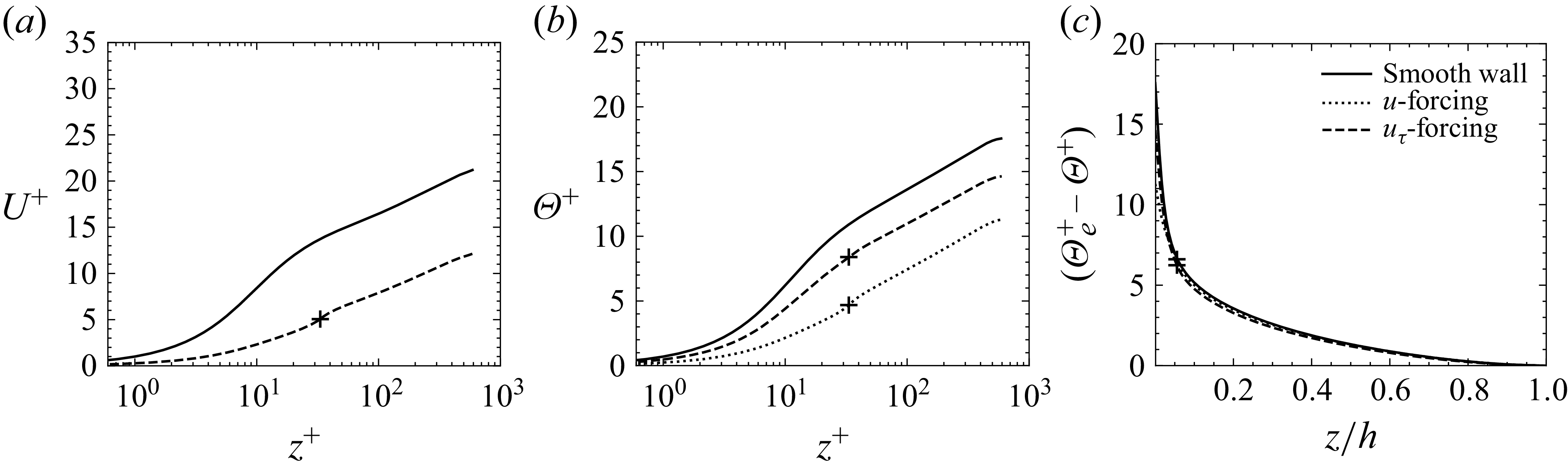
 k/h=1/18
 u
 uτ
 Reτ=590
 k+
 +
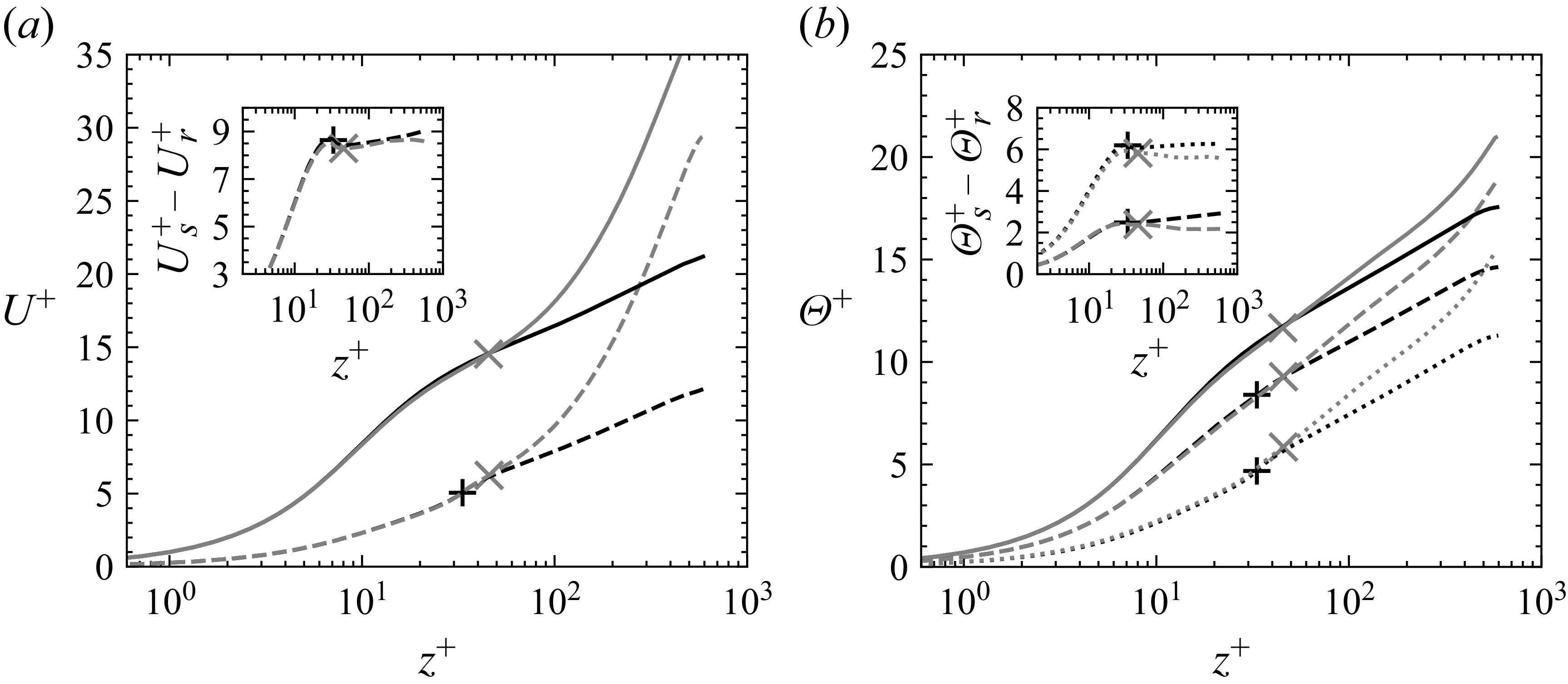
 k/h=1/18
 u
 uτ
 Reτ=590
 zc=0.4Ly
 ×
 k+
 +

 k+
 βk=βΘk=1/40
 βk=βΘk=1/18
 k/h=1/40
 k/h=1/18
 u
 uτ
 +
 ×
 zc+
 k+
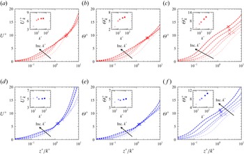
 z+/k+
 k+
 βk=βΘk=1/40
 βk=βΘk=1/18
 u
 uτ
 zc+
 k+

 βk=1/18
 βk=1/40
 ΔU+
 ΔΘ+
 k+
 ks+
 u
 uτ

 2Ch/Cf
 ks+
 log(z0m+/z0h+)
 z0m+

 ⟨τw,force⟩/⟨τw⟩
 Cf,k
 ⟨τw⟩/(1/2)ρUk2

 ks+
 ⟨τw,visc⟩
 ⟨τw,force⟩
 ⟨qw⟩
 βk=βΘk=1/40
 βk=βΘk=1/18
 ×
 (1/2)ρUk2
 ρCpUkΘk

 Ch,k
 ks+
 Ch,k,cond
 (ks+)−1/2
 Ch,k,force

 Ch,k
 ks+
 βk=βΘk=1/40
 βk=βΘk=1/18
 u
 uτ

 βΘk
 βk
 Reτ=590
 k+=33
 ΔΘ+
 k+
 βΘ/β=1
 βΘ/β=2

 k+
 Uk+
 Θk+
 k+
 2Ch/Cf
 k+
 Uk+
 +10
 (βk,βΘ/β)=(1/40,2)
 −0.2
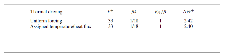
 ΔΘ+
 Reτ=590
 ΔΘ+
 uτ
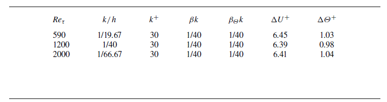
 ΔU+
 ΔΘ+
 ΔΘ+
 uτ

 Open access

