1. Introduction
PROTO-SPHERA is a magnetic confinement experiment, aimed at verifying the feasibility of axisymmetric plasmas in a simply connected magnetic configuration, i.e. without any solid structure placed between the plasma and the symmetry axis (Alladio et al. Reference Alladio, Costa, Mancuso, Micozzi, Papastergiou and Rogier2006; Lampasi et al. Reference Lampasi, Maffia, Alladio, Boncagni, Causa, Giovannozzi, Grosso, Mancuso, Micozzi and Piergotti2016). The simply connected plasma volume necessarily includes an unconfined region; in fact, as a consequence of the Poincaré–Hopf theorem, the confining part has to be toroidal (Hazeltine & Meiss Reference Hazeltine and Meiss1992). The PROTO-SPHERA configuration is formed by toroidal magnetic surfaces surrounding a pinch with open surfaces ending at electrodes. The pinch replaces solid structures that occupy the region around the symmetry axis in tokamaks. The overall plasma volume is then simply connected, while the confining portion is toroidal. The toroidal magnetic field is generated by current flowing in the central pinch, dubbed the centrepost discharge, which is fed by electrodes; external conductors that return the centrepost current are the only residual components of a toroidal magnet. The main goal of the experiment is to form and confine fat plasma tori around the centrepost discharge, in a steady-state magnetic configuration, i.e. without relying on image currents in conducting structures.
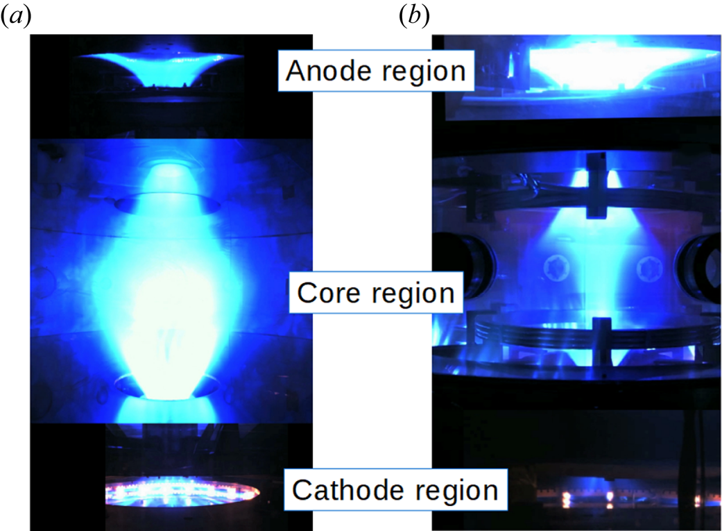
The centrepost discharge is shaped by eight poloidal magnetic field coils in order to wet large-area annular electrodes. The centrepost plasma appears as a pinch with variable diameter for a length of approximately 1 m and, after passing neck regions delimited by the bore of nearby shaping coils, it opens in the form of a mushroom in front of both annular electrodes (see figure 1a). The mushroom-shaped regions end with degenerate x-points (or triple nulls of the magnetic field) at the extremes along the axis. Compression coils, with current of opposite sign to that of shaping coils, balance the expansion force of current-carrying plasma tori. The centrepost bright plasma has a convex shape around the mid-plane when shaping coils only are activated. The bright region becomes concave as compression coils are activated, and a surrounding toroidal structure with different luminosity appears (see figure 1b).
Visible light images of PROTO-SPHERA plasmas in argon, as reconstructed from three cameras, one for the anodic region (top), one for the core region (middle) and one for the cathode region (bottom). View at the transitions between different regions is impeded by poloidal field coils.  $(a)$ Plasma configuration obtained with shaping coils only. The centrepost is convex in the core region and no torus is present; the mushroom-shaped region in front of the anode is uniform, while the cathodic one is filamented in correspondence with discrete electron emitters, which are visible as brilliant spots.
 $(b)$ Configuration with energised compression coils: the bright centrepost profile becomes concave, and a toroidal structure with different luminosity appears. Vision is further impeded in this setting by supporting structures of the compression coils.

The experiment is presently operated with a reduced-current version of the compression coils, in order to assess the capability of producing fat tori around 10 kA centrepost discharges. The target configuration, with centrepost current up to 70 kA and toroidal plasma current up to 300 kA, will become available after upgrading the compression coils as well as the power supplies.
Magnetic field maps can be obtained from numerical equilibrium calculations that include the actual shape of poloidal field coils; still, analytical models are desirable in order to provide a simple geometric basis for advanced studies of self-organisation of the configuration, in particular of how toroidal current can be sustained by magnetic reconnection in the absence of any applied toroidal electric field.
Analytical equilibrium models developed to reproduce at least locally the different observed PROTO-SPHERA topologies are described in this work. Equilibrium equations for simply connected axisymmetric equilibria are introduced in § 2. Solutions obtained by variable separation in cylindrical coordinates and models based on such solutions are presented in §§ 3 and 4, respectively. Solutions in spherical coordinates are obtained and and a model employing both cylindrical and spherical solutions is shown in § 5. Conclusions are given in § 6.
2. Equilibrium in PROTO-SPHERA axisymmetric plasmas
Some well-known results are reviewed in this section, in order to provide a basis to discuss additional constraints to be fulfilled by analytic solutions in simply connected configurations.
2.1. Axisymmetric fields
Axial symmetry implies the gradient operator along the azimuthal versor  $\boldsymbol {e}_{\phi }$ is null,
 ${\boldsymbol {e}_{\phi } \boldsymbol {\cdot } \boldsymbol {\nabla }=0}$, where
 $\phi$ is the azimuthal (or toroidal) angle. All quantities (excepting
 $\phi$) are constant on circles centred on the axis and lying on planes perpendicular to the axis. Poloidal magnetic flux (
 $\psi$) and poloidal current (
 $I$) linked by these circles are used to express the magnetic field in terms of scalar quantities and of
 $\boldsymbol {\nabla } \phi = \boldsymbol {e}_{\phi }/R$,
 $R$ being distance from the magnetic axis:
 \begin{equation} \boldsymbol{B} = \frac{1}{2 {\rm \pi}}\boldsymbol{\nabla} \psi \times \boldsymbol{\nabla}\phi + \frac{\mu_0 I}{2 {\rm \pi}} \boldsymbol{\nabla}\phi \equiv \boldsymbol{B}_{\textrm{pol}} + \boldsymbol{B}_{\textrm{tor}}. \end{equation}
The poloidal current  $I$ is entirely carried by the plasma in the simply connected case, whereas it includes current carried by toroidal magnet coils in the tokamak case.
The poloidal field component ( $\boldsymbol {B}_{\textrm {pol}}$) lies in poloidal cross-sections (in-plane with the symmetry axis) while the toroidal one (
 $\boldsymbol {B}_{\textrm {tor}}$) lies on planes perpendicular to the symmetry axis. Magnetic field lines lie on constant-
 $\psi$ surfaces (magnetic surfaces, or flux surfaces).
The current density reads
 \begin{equation} \boldsymbol{j} = \frac{1}{2{\rm \pi}}\boldsymbol{\nabla} I \times \boldsymbol{\nabla}\phi - \frac{R^2}{2{\rm \pi}\mu_0} \boldsymbol{\nabla}\boldsymbol{\cdot}\left(\frac{1}{R^2}\boldsymbol{\nabla}\psi \right) \boldsymbol{\nabla}\phi \equiv \boldsymbol{j}_{\textrm{pol}} + \boldsymbol{j}_{\textrm{tor}}. \end{equation}
Magnetic flux  $\psi$ and current
 $I$ are called poloidal flux and poloidal current, respectively, for having contributions from poloidal components only. Poloidal flux is related to the azimuthal component of the vector potential,
 $\psi =2{\rm \pi} R A_{\phi }$. In some textbooks the same symbol is used for poloidal flux divided by
 $2{\rm \pi}$.
The electromagnetic force density reads
 \begin{equation} \boldsymbol{j} \times \boldsymbol{B} = -\frac{1}{4{\rm \pi}^2\mu_0} \boldsymbol{\nabla}\boldsymbol{\cdot}\left(\frac{1}{R^2}\boldsymbol{\nabla}\psi \right) \boldsymbol{\nabla}\psi - \frac{\mu_0 I}{4{\rm \pi}^2 R^2} \boldsymbol{\nabla} I. \end{equation}
Here  $\boldsymbol {B} \boldsymbol {\cdot } \boldsymbol {j} \times \boldsymbol {B} = 0$ implies
 $\boldsymbol {\nabla } I \times \boldsymbol {\nabla } \psi = 0$; it follows that
 $I=I(\psi )$, i.e. poloidal current is a flux function, constant on flux surfaces. Derivatives of flux functions are indicated by a prime in the following:
 \begin{equation} I' \equiv \frac{\mathrm{d}I}{\mathrm{d}\psi}. \end{equation}
The gradient of poloidal current is
 \begin{equation} \boldsymbol{\nabla} I = I' \boldsymbol{\nabla}\psi. \end{equation}
2.2. The Grad–Shafranov equation
If inertial forces are negligible, the balance between electromagnetic force density and pressure gradient,
 \begin{equation} \boldsymbol{j} \times \boldsymbol{B} = \boldsymbol{\nabla} p,\end{equation}
implies  $\boldsymbol {B} \boldsymbol {\cdot } \boldsymbol {\nabla } p =0$. Since, by axisymmetry,
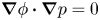 $\boldsymbol{\nabla}\phi\boldsymbol{\cdot}\boldsymbol{\nabla} p = 0$, it follows that
 $\boldsymbol {\nabla } p \times \boldsymbol {\nabla } \psi = 0$ and then pressure is a flux function,
 $p = p(\psi )$. In this condition, force balance can be expressed by the Grad–Shafranov (GS) equation:
 \begin{equation} \frac{1}{4{\rm \pi}^2\mu_0} \boldsymbol{\nabla}\boldsymbol{\cdot}\left(\frac{1}{R^2}\boldsymbol{\nabla}\psi \right) + \frac{\mu_0 I}{4{\rm \pi}^2 R^2} I'= - p', \end{equation}
where  $R$ is distance from the symmetry axis and primes denote derivatives with respect to
 $\psi$.
A generalised form of the GS equation (Lovelace et al. Reference Lovelace, Mehanian, Mobarry and Sulkanen1986) is required in the presence of substantial plasma flows. Toroidal rotation implies pressure is not a flux function and additional flux functions are needed to describe the plasma; furthermore, the operator structure changes if poloidal flow is present. The form (2.7) is used in the following; a study of the case with toroidal rotation is left to future work.
2.3. Linear models
Plasma equilibrium configurations are usually calculated via numerical solutions of the GS equation, assuming parametric functional forms of  $I(\psi )$ and
 $p(\psi )$ and determining parameters by iterative numerical schemes.
Exact analytical solutions of the GS equation have been used to benchmark numerical equilibrium codes, as well as to provide initial conditions for stability analysis in tokamaks. Exact tokamak equilibria have been found by assuming particular forms of the  $I(\psi )$ and
 $p(\psi )$ functions, for which the GS equation becomes linear (Solov'ev Reference Solov'ev1968; Guazzotto & Freidberg Reference Guazzotto and Freidberg2007; Xu & Fitzpatrick Reference Xu and Fitzpatrick2019). Wider families of solutions have been constructed by applying symmetry transformations (White & Hazeltine Reference White and Hazeltine2009).
Analytical equilibrium models are also desirable in the context of PROTO-SPHERA activities, in particular to provide a simple geometric basis for advanced studies of magnetic reconnection as well as of plasma transport. Analytical modelling of equilibrium in simply connected plasma configurations like PROTO-SPHERA entails consideration of solutions on a domain including the symmetry axis  $(R=0)$. For example, the choice of constant
 $I \, I'$, which gives compact and flexible solutions in the toroidal case (Solov'ev Reference Solov'ev1968; Xu & Fitzpatrick Reference Xu and Fitzpatrick2019), results in singular current density at
 $R=0$. The reason is that, being surface integrals of non-singular vector fields, both
 $\psi$ and
 $I$ should increase like
 $R^2$ near the axis, whereas constant
 $I\,I'$ implies
 $I\propto R$, i.e. singular poloidal current density.
The assumption on poloidal current adopted in this work is  $I\propto \psi$, i.e. constant
 $I'$, which linearises the GS equation while avoiding the singularity at the symmetry axis. The constant of proportionality is expressed in terms of the poloidal current parameter:
 \begin{equation} \mu=\mu_0 I'. \end{equation}
The assumption on  $p(\psi )$ is the same as in Solov'ev (Reference Solov'ev1968):
 \begin{equation} 4{\rm \pi}^2\mu_0 \, p'=\alpha, \end{equation}
where  $\alpha$ is a constant. In the force-free case (
 $\alpha =0$), the poloidal current parameter
 $\mu$ is equivalent to the Taylor relaxation parameter (Taylor & Turner Reference Taylor and Turner1989), whereas in general the poloidal current density only is relaxed:
 \begin{equation} \mu_0 \,\boldsymbol{j}_{\textrm{pol}} = \mu \boldsymbol{B}_{\textrm{pol}} ; \quad \mu_0 j_{\textrm{tor}} = \mu B_{\textrm{tor}} + \frac{\alpha R}{2 {\rm \pi}} . \end{equation}
With assumptions (2.8) and (2.9), the GS equation becomes
 \begin{equation} R^2 \boldsymbol{\nabla}\boldsymbol{\cdot}\left(\frac{1}{R^2}\boldsymbol{\nabla}\psi \right) + \mu^2\psi =- \alpha R^2. \end{equation}
Equilibrium models presented in the following sections involve combinations of solutions of the force-free equation
 \begin{equation} R^2 \boldsymbol{\nabla}\boldsymbol{\cdot}\left(\frac{1}{R^2}\boldsymbol{\nabla}\psi \right) + \mu^2\psi = 0 \end{equation}
with the particular solution of (2.11)
 \begin{equation} \psi_p = -\frac{\alpha}{\mu^2}R^2, \end{equation}
which, according to (2.1), corresponds to a uniform magnetic field parallel to the symmetry axis.
Equation (2.12) is separable both in cylindrical coordinates and in spherical ones. Solutions are developed in the following for each case, and simple models obtained by combining a few terms of the general solutions are discussed.
3. Equilibrium solutions in cylindrical coordinates
Equation (2.12) in  $(R, \phi , Z)$ cylindrical coordinates becomes
 \begin{equation} R \frac{\partial}{\partial R} \left( \frac{1}{R}\frac{\partial \psi}{\partial R} \right) + \frac{\partial^2 \psi}{\partial Z^2} + \mu^2 \psi = 0. \end{equation}
Magnetic field components are
 \begin{gather} B_R = -\frac{1}{2{\rm \pi} R}\frac{\partial \psi}{\partial Z}, \end{gather}
 \begin{gather}B_Z = \frac{1}{2{\rm \pi} R}\frac{\partial \psi}{\partial R}, \end{gather}
 \begin{gather}B_{\phi} = \frac{1}{2{\rm \pi} R}\mu\psi . \end{gather}
Separation of variables in the form  $\psi _n(R,Z)=Rf_n(R)g_n(Z)$, where the subscript labels individual solutions as determined by a separation parameter
 $k_n$, gives standard equations for
 $g_n$ and
 $f_n$:
 \begin{gather} \frac{\mathrm{d}^2 g_n}{\mathrm{d}Z^2} + k^2_n g_n = 0, \end{gather}
 \begin{gather} R^2 \frac{\mathrm{d}^2 f_n}{\mathrm{d}R^2} + R\frac{\mathrm{d}f_n}{\mathrm{d}R} + \left(\left(\mu^2 - k_n^2\right)R^2 -1\right) f_n = 0. \end{gather}
Real solutions of (3.3) are
 \begin{equation} g_n(Z) = \cos(k_n(Z-Z_n)), \end{equation}
showing that the  $k_n$ parameter introduced by separation is an inverse length scale in the axial direction.
Equation (3.4) is a Bessel equation for  $\mu \ne k_n$ and it reduces to an Euler equation for
 $\mu =k_n$; its real, non-singular solutions are
 \begin{gather} f_n(R)={\rm I}_1\left(\sqrt{|\mu^2-k_n^2|}\, R\right)/\sqrt{|\mu^2-k_n^2|} \quad \ \mathrm{as}\ \mu < k_n, \end{gather}
 \begin{gather}f_n(R)=R/2 \quad \mathrm{as}\ \mu=k_n, \end{gather}
 \begin{gather}f_n(R)={\rm J}_1\left(\sqrt{\mu^2-k_n^2}\, R\right)/\sqrt{\mu^2-k_n^2} \quad \mathrm{as}\ \mu>k_n, \end{gather}
where  ${\rm J}_1$ and
 ${\rm I}_1$ denote Bessel functions of the first kind and modified Bessel functions of the first kind, respectively, and denominators have been chosen to have continuity as
 $\mu /k_n$ changes. Solutions similar to (3.6c) were considered in Jensen & Chu (Reference Jensen and Chu1981) and Furth, Levine & Wantek (Reference Furth, Levine and Wantek1957).
Model equilibria can be constructed superposing individual solutions from (3.5), (3.6) and the particular solution (2.13):
 \begin{equation} \psi(R,Z) = \sum_{n=0} b_n R f_n(R) \cos(k_n(Z-Z_n)) - \frac{\alpha}{\mu^2}R^2. \end{equation}
The sum in (3.7) reduces to a Fourier series in  $Z$ if
 $k_n=nk_1$, i.e. if the separation parameters are multiples of a fundamental scale. A Fourier decomposition could then be used to obtain
 $b_n$ coefficients and
 $Z_n$ shifts for an assigned
 $Z$-profile of
 $\psi$ at constant
 $R$. A complementary approach is followed in this work, where the characteristics of up–down symmetric configurations (
 $Z_n=0$) obtainable with a few terms of the sum are studied for different values of the
 $b_n$ coefficients.
4. Equilibrium models in cylindrical coordinates
The topological features of equilibria that can be constructed from (3.7) can be illustrated considering just two terms of the sum. A periodic structure is obtained in this way, with a single period representing the core region as defined in figure 1. The mushroom-shaped regions are outside the scope of the present analysis. The force-free case ( $\alpha =0$) is considered first; the pressure term is then reintroduced at the end of this section.
The model with two terms is an extension of the bumpy pinch analytical model suggested by Taylor (Jensen & Chu Reference Jensen and Chu1981). The first term must have  $k_0=0$, as required to have open field lines around the
 $R=0$ axis. The second term must have
 $k_1={\rm \pi} /L$, where
 $L$ is the half-length of the core region. The origin of the
 $Z$ coordinate is chosen to have
 $Z_1=0$. Introducing the normalisation
 $\rho =k_1R$,
 $\zeta =k_1Z$,
 $\hat {\mu }=\mu /k_1$ and
 $\gamma _1=b_1/b_0$, the model flux takes a form that depends on
 $\hat {\mu }$ and
 $\gamma _1$ only:
 \begin{equation} \frac{k_1^2}{b_0} \psi(\rho,\zeta) = \frac{\rho}{\hat{\mu}} {\rm J}_1(\hat{\mu}\rho) + \gamma_1 \rho \hat{f}_1(\rho) \cos(\zeta), \end{equation}
where
 \begin{gather} \hat{f}_1(\rho)={\rm I}_1\left(\sqrt{|\hat{\mu}^2-1|}\, \rho\right)/ \sqrt{|\hat{\mu}^2-1|} \quad \mathrm{as}\ \hat{\mu}<1, \end{gather}
 \begin{gather}\hat{f}_1(\rho)=\rho/2 \quad \mathrm{as}\ \hat{\mu}=1, \end{gather}
 \begin{gather}\hat{f}_1(\rho)={\rm J}_1\left(\sqrt{\hat{\mu}^2-1} \rho\right)/ \sqrt{\hat{\mu}^2-1} \quad \mathrm{as}\ \hat{\mu}>1. \end{gather}
The topology of flux surfaces depends on the sign of  $\gamma _1$. Negative values correspond to magnetic configurations produced in the experiment by shaping coils only. Positive values correspond to configurations produced when compression coils are activated.
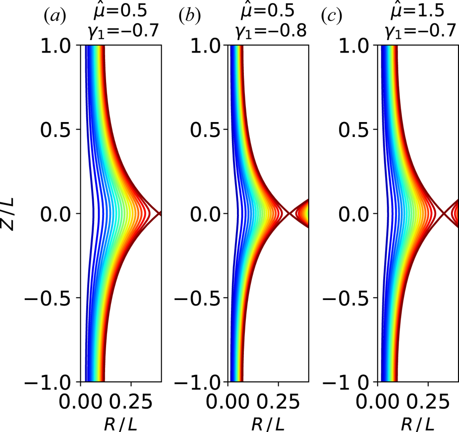
If  $\gamma _1<0$, there is a single x-point at the equatorial plane (see figure 2); all flux surfaces are open in this case and their shape is that of a bulge around the equatorial plane, consistent with the pinch-only experimental case shown in figure 1(a). The x-point location shifts inwards with increasing
 $\hat {\mu }$ as well as with increasing
 $|\gamma _1|$, as shown in figure 2.
Poloidal flux contour plots in a constant- $\phi$ (poloidal) cross-section for
 $\gamma _1<0$.
 $(a)$ Reference case with moderate values of both
 $\hat {\mu }$ and
 $|\gamma _1|$ parameters.
 $(b)$ Effect of larger
 $|\gamma _1|$.
 $(c)$ Effect of larger
 $\hat {\mu }$. Coordinates are normalised to half axial length,
 $R/L=\rho /{\rm \pi}$ and
 $Z/L=\zeta /{\rm \pi}$.

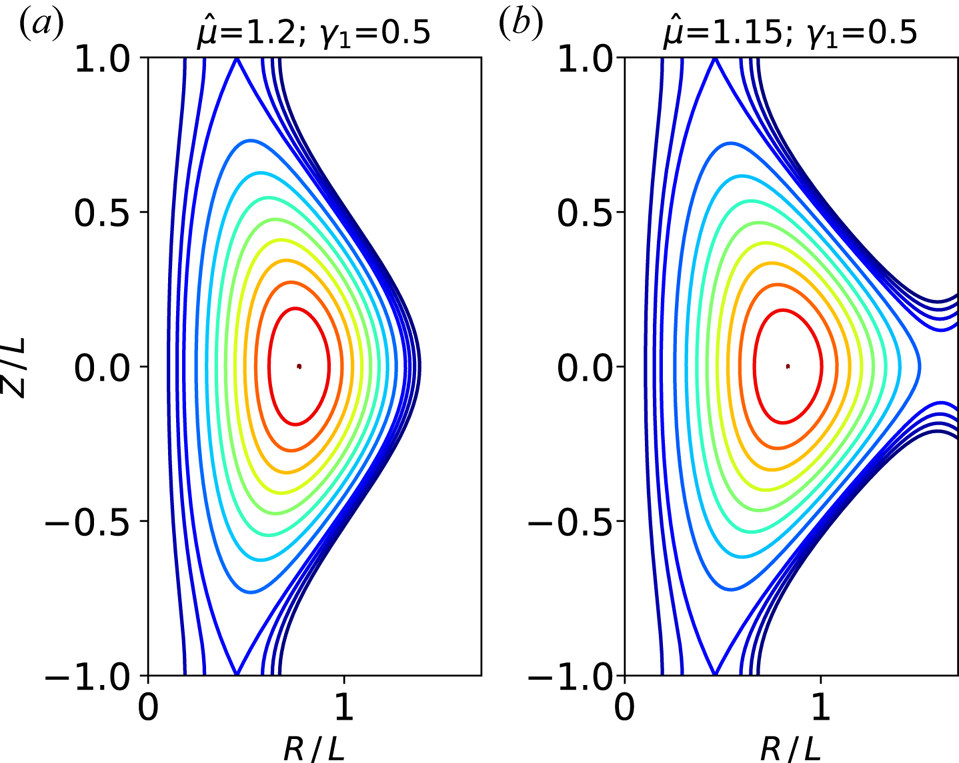
If in contrast  $\gamma _1>0$, an equatorial o-point surrounded by closed flux surfaces (i.e. a magnetic axis) appears, together with two x-points at
 $\zeta =\pm {\rm \pi}$, as shown in figure 3(a). Open flux contours appear squeezed around the equatorial plane, consistent with the experimental case shown in figure 1(b).
Poloidal flux contour plots in a constant- $\phi$ (poloidal) cross-section for
 $\gamma _1>0$.
 $(a)$ Configuration with
 $\hat {\mu }$ above the critical value: both branches of the separatrix between open and closed flux surfaces are continuous.
 $(b)$ Configuration with
 $\hat {\mu }$ slightly below the critical value: the outer separatrix branch breaks out. Coordinates are normalised to half axial length,
 $R/L=\rho /{\rm \pi}$ and
 $Z/L=\zeta /{\rm \pi}$.

This kind of configuration only exists if  $\hat {\mu }$ is above a critical value, otherwise the outer branch of the separatrix breaks out, as shown in figure 3(b). The critical value increases with
 $\gamma _1$, from 0.6 at
 $\gamma _1=0.01$ to 0.9 at
 $\gamma _1=0.1$ to 1.2 at
 $\gamma _1=0.5$. This indicates that the higher the applied compression field the more plasma current is required to form the configuration. The possibility of a localised equilibrium crisis in response to small variations of plasma current could play a role in plasma dynamics.
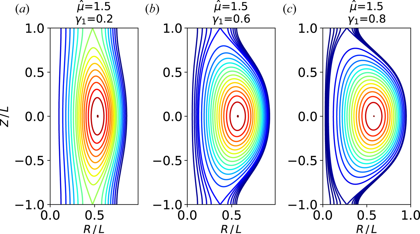
As  $\hat {\mu }$ increases above the critical value, the distance between the two branches of the separatrix decreases, i.e. elongation increases. The x-points shift inwards and the o-point slightly shifts outwards (i.e. triangularity increases) with increasing
 $\gamma _1$ at constant
 $\hat {\mu }$ (see figure 4).
Variation of plasma shape with (a–c) increasing  $\gamma _1$ at fixed
 $\hat {\mu }=1.5$ (well above the critical value). Coordinates are normalised to half axial length,
 $R/L=\rho /{\rm \pi}$ and
 $Z/L=\zeta /{\rm \pi}$.

When including a dimensionless form of the last term in (3.7), which represents finite plasma pressure, the model normalised flux becomes
 \begin{equation} \frac{k_1^2}{b_0} \psi(\rho,\zeta) = \frac{\rho}{\hat{\mu}} {\rm J}_1(\hat{\mu}\rho) + \gamma_1 \rho \hat{f}_1(\rho) \cos(\zeta) - \frac{1}{2{\rm \pi}}\beta \rho^2, \end{equation}
where the  $\beta$ parameter, defined as
 \begin{equation} \beta \equiv \frac{2{\rm \pi}\alpha}{b_0\mu^2}, \end{equation}
nearly (to within 20 %) equals the plasma beta  $2\mu _0 p / B^2$ at the magnetic axis. Triangularity increases with increasing
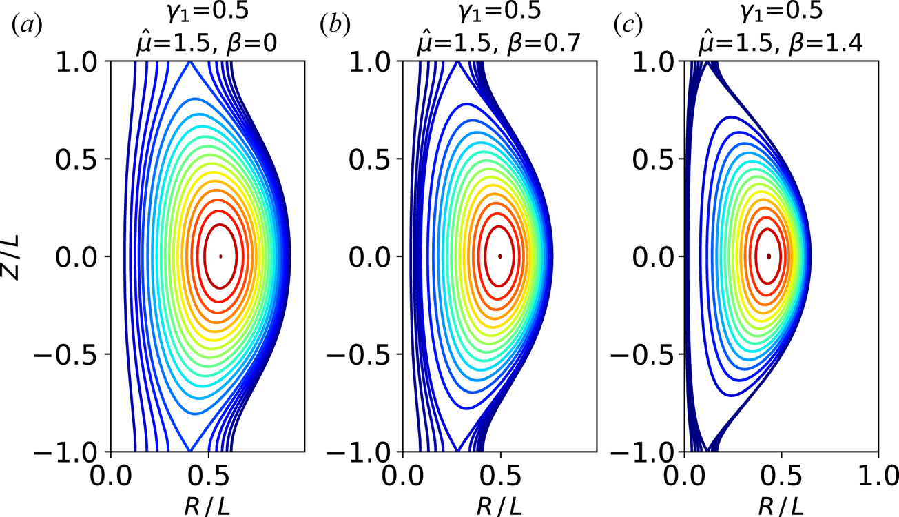
 $\beta$, as shown in figure 5, consistent with the fact that inclusion of finite plasma pressure adds a uniform
 $B_Z$ contribution, which tends to shift x-points towards the axis.
Poloidal flux contour plots in a constant- $\phi$ (poloidal) cross-section for increasing
 $\beta$ at constant values of both
 $\hat {\mu }$ and
 $\gamma _1$.
 $(a)$ Force-free case,
 $(b)$ intermediate
 $\beta$ and
 $(c)$
 $\beta$ close to the equilibrium limit. Coordinates are normalised to half axial length,
 $R/L=\rho /{\rm \pi}$ and
 $Z/L=\zeta /{\rm \pi}$.

The condition of the presence of open field lines gives restrictions on model parameters. Open field lines (which have to occupy a finite bore corresponding to the centrepost discharge) disappear as a zero appears in the axial profile of  $B_Z$. From (3.2b), using the derivation rules
 $(x{\rm J}_1(x))'=x{\rm J}_0$ and similar for
 ${\rm I}_1$:
 \begin{equation} B_Z(0,\zeta) = \frac{b_0}{2{\rm \pi}} \left(1 + \gamma_1 \cos(\zeta) - \frac{\beta}{{\rm \pi}} \right). \end{equation}
The condition 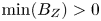 $\min (B_Z)>0$ gives both the equilibrium beta limit
 $\beta <{\rm \pi} (1-|\gamma _1|)$ and the shaping parameter limit in the force-free limit,
 $|\gamma _1|<1$.
5. Axially bounded equilibrium models
Equilibrium models obtained in the previous section do not attempt to reproduce the mushroom-shaped regions of the experimental configuration. Simple models with expansions that mimic such regions can be constructed by including a solution obtained by separation of variables in spherical coordinates.
5.1. Solutions in spherical coordinates
Equation (2.12) in  $(r,\theta ,\phi )$ spherical coordinates, where
 $r=(R^2+Z^2)^{1/2}$ and
 $\tan \theta =R/Z$, takes the form
 \begin{equation} \frac{\partial^2 \psi}{\partial r^2}+ \frac{\sin\theta}{r^2}\frac{\partial}{\partial \theta} \left( \frac{1}{\sin\theta}\frac{\partial \psi}{\partial \theta} \right) + \mu^2 \psi = 0. \end{equation}
Separation of variables  $\psi _n(r,\theta )=\psi _{n1}(r)\,\psi _{n2}(x)$, with
 $x=\cos \theta$, gives
 \begin{equation} \frac{r^2}{\psi_{n1}} \frac{\mathrm{d}^2 \psi_{n1}}{\mathrm{d} r^2} + r^2 \mu^2 = - \frac{1-x^2}{\psi_{n2}} \frac{\mathrm{d}^2 \psi_{n2}}{{\textrm{d}x}^2} = n(n+1), \end{equation}
where  $n$ is a separation parameter. With the change of variable
 $\psi _{n2}=(1-x^2)^{1/2}p(x)$, the angular part of (5.2) becomes a general Legendre equation of degree
 $n$ and order 1, with solution
 $p(x)=-P_n^1(x)$, where the negative sign is used for consistency with Rogier et al. (Reference Rogier, Bracco, Mancuso, Micozzi and Alladio2003). For integer
 $n$ the angular dependence becomes a combination of Legendre polynomials:
 \begin{equation} \psi_{n2}(x) = nP_{n-1}(x) - nxP_n(x). \end{equation}
The equation for the radial dependence transforms into a Bessel equation with the change of variable  $\psi _{n1}(r)=\mu r q(r)$. The solution for integer
 $n$ is a spherical Bessel function,
 $q(r) = j_n(\mu r)$, so that the generic solution for integer
 $n$ is
 \begin{equation} \psi_n(r,\theta) = \mu r j_n(\mu r) (nP_{n-1}(\cos\theta) - n\cos\theta P_n(\cos\theta)). \end{equation}
Equivalent solutions have been obtained in Chandrasekhar (Reference Chandrasekhar1956) and Chandrasekhar & Kendall (Reference Chandrasekhar and Kendall1957). The  $n=1$ solution is used in the next subsection.
5.2. The Chandrasekhar–Kendall–Furth model
The  $n=1$ spherical solution, indicated as
 $\psi _{\textrm {spher}}$ in the following, can be modified to reproduce some global aspects of PROTO-SPHERA equilibria (Rogier et al. Reference Rogier, Bracco, Mancuso, Micozzi and Alladio2003), in particular the presence of a core plasma region and of two mushroom-shaped expansions in front of the electrodes, connected to the core region by relatively narrow sections. Another reproduced feature is the presence of triple nulls of the magnetic field at the extremes along the axis of the mushroom-shaped parts.
Using explicit expressions of  $P_0$ and
 $P_1$, the
 $n=1$ spherical solution takes the simple form
 \begin{equation} \psi_{\textrm{spher}}(r,\theta) = \mu r j_1(\mu r) \sin^2\theta, \end{equation}
or, in cylindrical coordinates,
 \begin{equation} \hat{\psi}_{\textrm{spher}}(R,Z) = j_1(\mu (R^2+Z^2)^{1/2}) \mu R^2/(R^2+Z^2)^{1/2}. \end{equation}
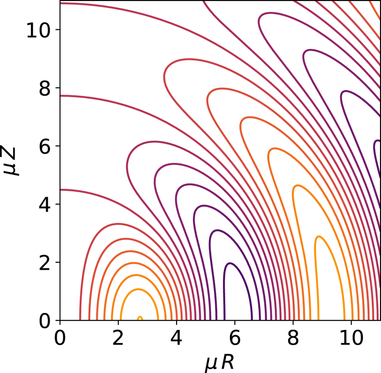
Contour plots of (5.6) are shown in figure 6. Three regions with closed flux surfaces, separated by zeros of  $j_1(\mu r)$ at
 $\mu r_1\approx 4.4934$,
 $\mu r_2\approx 7.7253$ and
 $\mu r_3\approx 10.9041$, can be seen in figure 6, where boundary lines appear as quarters of a circle intersecting the
 $Z$ axis. Points of intersection with the
 $Z$ axis are triple magnetic nulls. The inner region (with positive flux, ending at
 $r=r_1$) can be modified to reproduce the core plasma (as defined in figure 1), provided that some of its surfaces become connected with ones of the outer region. The outer region (
 $r_2 < r < r_3$, again with positive flux) can then be transformed into the expanded centrepost in front of the electrodes (the configuration is up–down symmetric, the upper part only being shown in figure 6). The negative-flux region in the middle (
 $r_1 < r < r_2$) gives rise to the neck regions lying between core plasma and expanded centrepost regions. This topological change can be accomplished by superposing a different equilibrium solution to (5.5), in order to introduce a bridge with positive flux across the negative-flux region. An additional requirement is to preserve the presence of a triple magnetic null at the end of the configuration along the axis. Both requirements can be fulfilled by superposing a solution having the form presented in § 3:
 \begin{equation} \psi_{\textrm{cyl}}(R,Z) = (\mu^2-k^2)^{1/2} R {\rm J}_1((\mu^2-k^2)^{1/2} R) \cos(k Z), \end{equation}
with
 \begin{equation} k=\frac{{\rm \pi}}{2 x_3} \mu, \end{equation}
such that the triple null of  $\psi _{\textrm {cyl}}$ coincides with the third null of
 $\psi _{\textrm {spher}}$. A constant factor has been introduced in (5.7) for consistency with
Constant-poloidal-flux contours for the  $n=1$ solution obtained from separation of variables in spherical coordinates. Coordinates
 $R=r\sin \theta$ and
 $Z=r\cos \theta$ are normalised by the length scale associated with the poloidal current parameter. Hot colours correspond to positive values.

Rogier et al. (Reference Rogier, Bracco, Mancuso, Micozzi and Alladio2003). The  $n$ subscript has been removed in (5.7) since a single
 $k$ is involved, and the
 $\mu >k$ form of (3.6) has been used, consistent with (5.8).
The superposition of (5.5) and (5.7),
 \begin{equation} \psi_{\textrm{CKF}} = \hat{\psi}_{\textrm{spher}}+\gamma\,\psi_{\textrm{cyl}}, \end{equation}
where  $\gamma$ is the superposition coefficient, has been dubbed (Rogier et al. Reference Rogier, Bracco, Mancuso, Micozzi and Alladio2003) the Chandrasekhar–Kendall–Furth force-free field (CKF), for being based on particular equilibrium solutions from Chandrasekhar & Kendall (Reference Chandrasekhar and Kendall1957) and Furth et al. (Reference Furth, Levine and Wantek1957).
The shape of CKF configurations does not depend on the poloidal current parameter; in fact  $\mu$ variations are equivalent to rescaling both
 $R$ and
 $Z$ with the same factor. The dimensional half-length of the configuration, defined as the distance between the origin and each of the triple null points, is
 $L=x_3/\mu$.
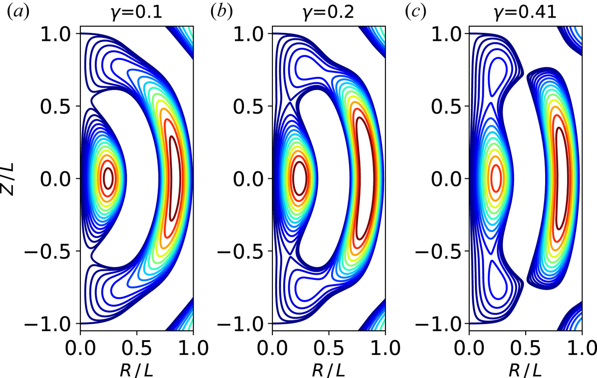
The CKF configurations change markedly as the  $\gamma$ superposition coefficient increases. A representative sequence is shown in figure 7. For
 $\gamma =0.1$ (see figure 7a), some contours that surround both positive-flux regions appear, and the tips of these regions come in contact at two x-points (only visible upon zooming), while the negative-flux region, which is represented by a white area, becomes detached from the
 $Z$ axis. For
 $\gamma =0.2$, contours lying between the separatrix and the
 $Z$ axis become evident (see figure 7b). Their shape resembles visible camera images of the centrepost discharge, particularly for the rapid turning in proximity of triple null points. Meanwhile, the outer positive region tends to break, as shown by the appearance of some throttled contours. For
 $\gamma >0.402$, the outer positive region breaks apart, resulting in a configuration with two closed secondary tori on the top and bottom of the main torus (see figure 7c). This kind of configuration was used in Rogier et al. (Reference Rogier, Bracco, Mancuso, Micozzi and Alladio2003) as a basis for ideal magnetohydrodynamic stability studies, as well as for conceptual studies of plasma propulsion. Secondary tori completely merge with the main torus as
 $\gamma$ increases above
 $0.69$.
Constant-flux contours of CKF models with superposition coefficient  $(a)$
 $\gamma =0.1$,
 $(b)$
 $\gamma =0.2$ and
 $(c)$
 $\gamma =0.41$. Coordinates are normalised to half axial length. Regions with negative flux appear as white areas, as negative contour levels are not shown.

Equilibrium models based on the CKF configuration complement the ones presented in § 3, for being less flexible but more global.
6. Concluding remarks
Analytical models of PROTO-SPHERA equilibria have been developed in order to provide a simple geometric basis for studies of self-organisation of the configuration.
The GS equilibrium equation has been linearised adopting prescriptions to fulfil regularity of solutions in a domain that includes the symmetry axis, as required to model PROTO-SPHERA simply connected configurations.
Particular solutions obtained with separation of variables in cylindrical coordinates have been used to construct a simple equilibrium model, which can locally (in the plasma core region) reproduce different plasma topologies that can be observed in the experiment. This model shows a criticality of equilibrium topology, due to breakout at low plasma current of the outer branch of the separatrix between closed and open flux surfaces, an effect that could play a role in plasma dynamical processes.
Other solutions have been obtained with separation of variables in spherical coordinates. A model that allows reproduction of the presence of three different plasma regions (anodic, core and cathodic) in the actual PROTO-SPHERA configuration has been implemented by combining a spherical solution with a cylindrical one.
Editor William Dorland thanks the referees for their advice in evaluating this article.
Declaration of interests
The authors report no conflict of interest.