SPATIAL, TEMPORAL AND SPATIOTEMPORAL INTERDEPENDENCE IN BINARY-OUTCOME MODELS

Many phenomena that social scientists study are inherently, or by measurement, discrete choices. Canonical political science examples include citizens’ vote and turnout choices, legislators’ votes, governments’ policy enactments, wars among or within nations, and regime type or transition. In all these contexts, and widely across the political and social sciences, the outcomes in some units depend substantively and theoretically importantly on those of other units.Footnote ¹ Scholars argue, for example, that whether and for whom citizens vote depend on whether and how their neighbors or social networks vote; that each legislator’s vote depends on how s/he expects or observes others to vote; that governments’ policy choices depend on others’ policies via competition and learning; that states’ entry to and involvement in external wars, international organizations, and treaties are heavily conditioned by whether and which ones other states join; and that regime change at home or, as in our own empirical application below, nations’ internal wars are often spurred by example, fomentation or otherwise from abroad. Nevertheless, in most research areas, spatial (that is, cross-unit) interdependence in discrete outcomes receives very little direct empirical attention.Footnote ² Even when researchers have attempted to explicitly account interdependence empirically, the inappropriate estimation strategies usually employed have rendered their estimates unreliable. Unlike cross-unit interdependence, the over-time dependence of binary outcomes has received considerable attention—and, consequently, has seen more-effective indirect empirical-modeling strategies developed—yet modeling temporal auto-dependence directly raises these same methodological challenges. Auto-dependence in binary outcomes, across space and/or over time, requires strategies for modeling simultaneous spatial and/or temporal lags of the latent outcomes (that is, the underlying propensities toward the binary outcome), which is methodologically challenging to do. This article discusses a simulation-based strategy for estimating these auto-dependence parameters directly in spatiotemporally autoregressive binary-outcome models and, we believe for the first time, for calculating substantively meaningful conditional spatiotemporal effects and response paths in terms of outcome probabilities.

While efforts to model spatial interdependence directly in binary outcomes have recently expanded in some contexts, the strategies employed often fail to account for the endogeneity induced by including spatial lags. Using our example application from below to illustrate: Senegal is on Guinea-Bissau’s right-hand side, the former affecting the probability of internal conflict in the latter, but, simultaneously, Guinea-Bissau is on Senegal’s right-hand side, affecting its probability of civil war. Moreover, placing the actual binary outcomes of other units (or weighted sums or averages of actual outcomes) simultaneously on the right-hand side is not algebraically consistent (Heckman Reference Hegre, Ellingsen, Gates and Gleditsch1978). Such simultaneity can only logically operate through the latent variables or errors, which raises additional econometric and computational challenges. Diffusion researchers often time lag these spatial lags in an attempt to bypass these issues. While this can suffice to evade the simultaneity bias (Beck, Gleditsch and Beardsley Reference Beck, Gleditsch and Beardsley2006), its efficacy in doing so rests on the assumptions (we believe frequently untenable) that: (1) the interdependence does not occur instantaneously, that is, within an observational period, (2) the actual periodicity and lag structure match that of the empirical observations and specification and (3) the empirical model of spatiotemporal dynamics is adequate to prevent the past bleeding into the present through mismeasurement and/or misspecification.Footnote ³ Should any of these conditions fail, time lagging spatial lags will be technically inappropriate and practically insufficient to redress the spatial-lag endogeneity.

That outcomes will auto-correlate over time requires no parallel introduction or argument. No one would argue or pretend that time-serial observations were temporally independent in almost any context. Yet because temporal auto-dependence affords some simple evasions that spatial interdependence does not, empirical applications that model temporal auto-dependence directly are rarer still. Instead, researchers mostly follow Beck, Katz and Tucker’s (Reference Beck, Katz and Tucker1998) or Carter and Signorino’s (2010) advice to sidestep the estimation challenges by modeling temporal trends with flexible functions of time-since-event instead. Such time dependence is not quite auto-dependence of a unit’s current propensity on its previous propensities, so while these approaches may adequately correct the biases and exaggerated certainty estimates that stem from falsely pretending that time-serial binary observations are independent, they do not offer a direct model of temporal-autoregressive processes.Footnote ⁴ Some researchers have instead shifted strategy and focus to model, not the outcomes directly, but transition matrices of state-switching probabilities (that is, probabilities of switching or staying in states 0 or 1) conditional on the previous observed state (for example, Jackman Reference Kathman2000; Przeworski et al. 2000; Beck et al. Reference Beck, Epstein, Jackman and O’Halloran2001).Footnote ⁵ This is autoregression in the binary outcome (and therefore a fuller strategy for temporal auto-dependence) but modeling interdependence directly in the latent propensities may be more appealing substantively in some contexts, and affords estimation of models in more-familiar standard binary-outcome format, without shifting strategy and focus.

Working under the incorrect assumption of spatial, temporal or spatiotemporal independence yields overconfidence and inefficiency at best, and usually bias and inconsistency too. Moreover, while including spatial and/or temporal lags to reflect (inter)dependence directly is advisable, simultaneous spatial lags are endogenous, and thus introduce biases if entered as right-hand-side variables in estimation procedures, like standard logit/probit, that assume their exogeneity (for example, Franzese and Hays Reference Franzese and Hays2004, Reference Franzese and Hays2007, 2008).Footnote ⁶ Therefore, we suggest a simulation-based approach for estimating models with simultaneous spatial and temporal lags (STP) of the latent outcomes using maximum simulated likelihood (MSL) by recursive-importance sampling (RIS), stated together as STP-MSL-by-RIS. This strategy enables us to recover not only accurate parameter estimates but also, more importantly, estimates of substantive conditional spatiotemporal effects, response paths and long-run-steady-state responses. Ultimately, we are interested in how probabilities of outcomes in this and other units and times respond to hypothetical changes in explanatory factors (X’s), propensities (y*), or outcomes (y) in this and other units and times. Yet extant empirical studies, even those few works that attempt to model spatial interdependence directly and, within those, even those rarer ones that apply appropriate estimation strategies to do so, tend to ignore such substantive effects, instead simply relying on parameter estimates (and significance) as evidence of spatial-effect existence, which, even when properly estimated, offer little sense of effect magnitude given the non-linearities of the spatial multiplier and the binary-outcome probability. Likewise, current strategies for modeling time dependence do not (or at least do not easily) enable us to calculate response paths over time or long-run effects in substantive terms. Simulation-based strategies like STP-MSL-by-RIS enable direct estimation of spatiotemporal autoregressive processes and of substantive spatiotemporal effects, response paths and steady states, all in terms of (conditional) probabilities of outcomes. We can calculate, for example, how a hypothetical increase in the propensity toward internal conflict or change in the realized outcome itself in Senegal (and/or elsewhere) affects the probability of civil war in Guinea-Bissau (and/or elsewhere) simultaneously, over time, and in the long run, including all spatiotemporal feedback between each other and around the Sub-Saharan state system in all time periods.

The article proceeds as follows: first, we briefly explain (with technical details and elaboration relegated to web appendices): (1) the severe inferential challenges posed by spatial, temporal or spatiotemporal interdependence in binary outcomes and (2) recent spatial-econometric advances using simulation-based methods to surmount the analytical challenges that arise in such problems. Next, Monte Carlo simulations compare the performance of one such consistent and asymptotically efficient method (STP-MSL-by-RIS) to estimation strategies naïve about (inter)dependence—that is, including lags but treating them as exogenous regressors in standard probit estimation. Penultimately, we show—we believe for the first time—how to calculate spatiotemporal response paths in outcome probabilities (with associated uncertainty estimates) for some units from hypothetical changes to outcomes in other units. Finally, we illustrate with an application to civil war in Sub-Saharan Africa and conclude.

THE ECONOMETRIC PROBLEM

Methods for properly estimating and analyzing models of interdependent binary outcomes have received significant attention in the spatial-econometric literature recently. Most of this research considers the spatial-probit model with interdependence in the latent variable—that is, in the unobserved argument to the probit-modeled probability of a binary outcome.Footnote ⁷ Several estimation strategies have been suggested. We focus on simulated-likelihood strategies and, in particular, the RIS estimator advanced by Beron, Murdoch and Vijverberg (Reference Beron, Murdoch and Vijverberg2003) and Beron and Vijverberg (Reference Beron and Vijverberg2004).Footnote ⁸ In brief, interdependence in binary outcomes necessitates simulation-based estimation strategies, STP-MSL or MCMC, because the dependence across observations invalidates the typical process of deriving the overall likelihood (posterior) to be maximized by multiplying the probabilities (adding the log-likelihoods) of each observation; independence is required for that step. Interdependence instead leaves one n-dimensional distribution in the likelihood (posterior)—in the spatial-probit case, a truncated cumulative multivariate normal distribution—to maximize, which is difficult and computationally intense. We now review the spatial-probit model closely and then show how probit with temporal or spatiotemporal dependence in the latent variable is very similar in form, indicating that the same empirical strategies can apply there.

The structural model for the latent variable of the spatial probit takes the form:

(1) $${\bf y}{\!\asterisk}=\rho {\bf Wy}{\!\asterisk}\!{\plus}{\bf X\bbeta }{\plus}{\bf {\bvarepsilon}},$$

where Wy* is the spatial lag, and W the all-important spatial-connectivity matrix, with element w _ij giving the relative connectivity from unit j to i. The ρ, which is to be estimated, is the strength of interdependence by that pattern given in W. The model (1) can be rewritten in reduced form as:

(2) $${\bf y}{\!\asterisk}=({\bf I}{\minus}\rho {\bf W})^{{\!{\minus}\!1}} {\bf X\bbeta }{\plus}{\bf u}{\rm ,}\,{\rm with}\,{\bf u}=({\bf I}{\minus}\rho {\bf W})^{{\!{\minus}\!1}} {\bf {\bvarepsilon}}.$$

Latent-variable y* links to the observed binary outcome, y, through the measurement equation:

(3) $$y_{i} =\{ 1\,{\rm if}\,y_{i} {\!\asterisk}\,\gt\, 0\,{\rm ;}\,{\rm 0}\,{\rm if}\,y_{i} {\!\asterisk}\!\leq \,0\} .$$

The probability that the ith observation equals 1 is calculated as follows:Footnote

(4) $$\eqalignno{ p(y_{i} =1\!\mid\!{\bf X})=\ & p\left( {\left[ {({\bf I}{\minus}\rho {\bf W})^{{\!{\minus}\!1}} {\bf X\bbeta }} \right]_{i} {\plus}\left[ {({\bf I}{\minus}\rho {\bf W})^{{\!{\minus}\!1}} {\bf {\bvarepsilon}}} \right]_{i} \;\gt \;0} \right) \cr =\ & p\left( {u_{i} \lt \left[ {({\bf I}{\minus}\rho {\bf W})^{{\!{\minus}\!1}} {\bf X\bbeta }} \right]_{i} } \right)=\Phi \left\{ {{{\left[ {({\bf I}{\minus}\rho {\bf W})^{\!{{\minus}\!1}} {\bf X\bbeta }} \right]_{i} } \mathord{\left/ {\vphantom {{\left[ {({\bf I}{\minus}\rho {\bf W})^{{{\minus}1}} {\bf X\beta }} \right]_{i} } {\sigma _{{u_{i} }} }}} \right. \kern-\nulldelimiterspace} {\sigma _{{u_{i} }} }}} \right\}. \qquad\qquad\quad \ \ \qquad (4)^9$$

Thus, as in the standard probit, a cumulative-normal distribution, $\Phi \left\{ \zrad \right\}$ , gives the probability that the systematic component, [(I−ρ W)⁻¹XP]_i, exceeds the stochastic component, u _i. (The division by $\sigma _{{u_{i} }}^{2} $ occurs here because u, unlike ε, is heteroskedastic.) The interdependence of the y _i* in spatial probit induces a nonsphericity of the reduced-form stochastic components, u. Specifically, u is distributed n-dimensional multivariate normal with mean 0 and variance-covariance [(I−ρ W)′(I−ρ W)]⁻¹. Intuitively, start with the standard (nonspatial) probit: ε is multivariate normal with mean 0 and spherical variance-covariance $\sigma ^{2} {\bf I}$ , and $\sigma ^{2} $ is normalized to 1. Then:

(5) $$\eqalignno{ V[{\bf u}]\,\equiv\,{\bf \Sigma }=V[({\bf I}{\minus}\rho {\bf W})^{\!{{\minus}\!1}} {\bf {\bvarepsilon}}]= & [({\bf I}{\minus}\rho {\bf W})^{\!{{\minus}\!1}} ]'V({\bf {\bvarepsilon}})[({\bf I}{\minus}\rho {\bf W})^{{\!{\minus}\!1}} ] \cr = & [({\bf I}{\minus}\rho {\bf W})^{\!{{\minus}\!1}} ]'{\bf I}[({\bf I}{\minus}\rho {\bf W})^{\!{{\minus}\!1}} ]=[({\bf I}{\minus}\rho {\bf W})'({\bf I}{\minus}\rho {\bf W})]^{{\!{\minus}\!1}} . $$

Thus the $\sigma _{{u_{i} }}^{2} $ in (4) is the iith element of variance-covariance (5), which is not a constant (such as 1 in standard probit). That is, interdependence also induces heteroskedasticity. This heteroskedasticity and, more crucially, the interdependence (that is, the non-independence) of the u _i render standard probit inappropriate and create the computational intensity. With the outcomes interdependent, their joint likelihood to be maximized is not the product (sum) of n independent univariate marginal (log) distributions; instead, one must maximize the log of one non-separable n-dimensional distribution. Finally, notice also that the ith observation probability depends on the entire matrix X and vector ε. The probability of Civil War in Senegal depends on the propensities toward internal conflict, and thus the full set of systematic and stochastic features in the entire Sub-Saharan state system. This follows from the nonlinearity of the sigmoidal probit function, which implies that effects depend on where along the S-shape they occur, and where on that S-curve one lies depends on all of X and all of ε, given the dependence of $y_{i}^{{\!\asterisk}} $ on Wy*.Footnote ¹⁰

Consider now the similarity of a probit model with temporal auto-dependence, say an AR(1) process, in the latent variable. Start with the structural model in matrix notation:

(6) $${\bf y}{\!\asterisk}=\phi {\bf Ly}{\!\asterisk}\!{\plus}{\bf X\bbeta }{\plus}{\bf {\bvarepsilon}}.$$

With y* a T×1 vector of latent variables, L a matrix of 0’s except for all 1’s on the lower first-minor diagonal (the diagonal just below the prime diagonal) and dropping the first observation,Footnote ¹¹ this gives a standard first-order temporal autoregressive model, with reduced form:

(7) $${\bf y}{\!\asterisk}\!=({\bf I}{\minus}\phi {\bf L})^{{\!{\minus}\!1}} {\bf X\bbeta }{\plus}{\bf u}{\rm ,}\,{\rm with}\,{\bf u}=({\bf I}{\minus}\phi {\bf L})^{{\!{\minus}\!1}} {\bf {\bvarepsilon}}.$$

Again, this implies a nonspherical variance-covariance of the form:

(8) $$V[{\bf u}]\,\equiv\,{\bf \Sigma }=V[({\bf I}{\minus}\phi {\bf L})^{\!{{\minus}\!1}} {\bf {\bvarepsilon}}]=[({\bf I}{\minus}\phi {\bf L})^{\!{{\minus}\!1}} ]'V({\bf {\bvarepsilon}})[({\bf I}{\minus}\phi {\bf L})^{{\!{\minus}\!1}} ]=[({\bf I}{\minus}\phi {\bf L})'({\bf I}{\minus}\phi {\bf L})]^{\!{{\minus}\!1}} ,$$

and the rest of the discussion regarding the estimation and interpretation complications that come with this nonseparable T-dimensional cumulative nonspherical normal distributions apply mutatis mutandis. For the panel or time-series-cross-section case with spatial and temporal lag, we could write:

(9) $${\bf y}{\!\asterisk}\!=\rho {\bf Wy}{\!\asterisk}\!{\plus}\phi {\bf Ly}{\!\asterisk}\!{\plus}{\bf X\bbeta }{\plus}{\bf {\bvarepsilon}}.$$

Ordering the data by period, units 1 to N in time 1 through to units 1 to N in time T, and dropping period 0, W is now an NT×NT matrix with N×N submatrices W_t with elements w _ij giving relative connectivity from unit j to unit i, period by period down the block diagonal, and L is an NT×NT matrix of 0’s except with 1’s on the diagonal of the lower block first-minor (that is, with N×N identity matrices along the blocks just below the prime block-diagonal), making Ly* the within-unit one-period time lag of y*. The reduced form is now:

(10) $${\bf y}{\!\asterisk}\!=({\bf I}{\minus}\rho {\bf W}{\minus}\phi {\bf L})^{\!{{\minus}\!1}} {\bf X\bbeta }{\plus}{\bf u}{\rm ,}\,{\rm with}\,{\bf u}=({\bf I}{\minus}\rho {\bf W}{\minus}\phi {\bf L})^{\!{{\minus}\!1}} {\bf {\bvarepsilon}},$$

which again implies a nonspherical variance-covariance for u, similar in form:

(11) $$V[{\bf u}]\,\equiv\,{\bf \Sigma }=V[({\bf I}{\minus}\rho {\bf W}{\minus}\phi {\bf L})^{\!{{\minus}\!1}} {\bf {\bvarepsilon}}]=[({\bf I}{\minus}\rho {\bf W}{\minus}\phi {\bf L})'({\bf I}{\minus}\rho {\bf W}{\minus}\phi {\bf L})]^{\!{{\minus}\!1}} .$$

We will focus on this simultaneous spatiotemporal-lag model (dropping the first time periods) next because it raises the estimation and interpretation issues fully, and the reduction to the simple cross-section or time-series is a straightforward.

THE MAXIMUM SIMULATED-LIKELIHOOD (STP-MSL) BY RECURSIVE IMPORTANCE SAMPLER (RIS) ESTIMATOR FOR SIMULTANEOUS SPATIAL, TEMPORAL OR SPATIOTEMPORAL PROBIT

We discuss STP-MSL strategies, and in particular the RIS estimator for spatial probit advanced by Beron, Murdoch and Vijverberg (Reference Beron, Murdoch and Vijverberg2003) and Beron and Vijverberg (Reference Beron and Vijverberg2004).Footnote ¹² The same equations and procedures apply for the spatial-, temporal- and spatiotemporal-autoregressive cases, simply using (I−ρ W)⁻¹, (I−ϕ L)⁻¹ or (I−ϕ L−ρ W)⁻¹ as appropriate for the multipliers, as seen in Equations 2–11 above.

RIS uses simulation to approximate probabilities that are difficult to calculate analytically, such as those from the cumulative multivariate normal distributions unavoidably introduced by the interdependence in spatial, temporal or spatiotemporal probit.Footnote ¹³ To approximate a cumulative multivariate-normal distribution such as the following, for example,

(12) $$p=\mathop{\int}\limits_{{\minus}\infty}^{{\bf x}_{0} } {f_{n} ({\bf x}){\rm }d{\bf x}} ,$$

where $$f_{n} \left( {\bf x} \right)$$ is the density and $\left[ {{\minus}\infty,{\bf x}_{0} } \right]$ the interval over which we want to integrate, we first choose an n-dimensional sampling distribution with well-known properties and label a truncation of this sampling distribution with support over $\left[ {{\minus}\infty,{\bf x}_{0} } \right]$ the importance distribution. Multiplying and dividing the right-hand side of the integral we wish to calculate, Equation 12, by the density of this importance distribution, $g_{n}^{c} \left( {\bf x} \right)$ , simply restates Equation 12 as:

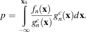(13) $$p=\mathop{\int}\limits_{{\minus}\infty}^{{\bf x}_{0} } {{{f_{n} ({\bf x})} \over {g_{n}^{c} ({\bf x})}}{\rm }g_{n}^{c} ({\bf x}){\rm }d{\bf x}} .$$

By definition, because $g_{n}^{c} \left( {\bf x} \right)$ is a valid pdf over the integral’s range, this integral is a mean. Thus Equation 13 gives the probability sought, p, as the mean of $${{f_{n} ({\bf x})} \mathord{\left/ {\vphantom {{f_{n} ({\bf x})} {g_{n}^{c} ({\bf x})}}} \right. \kern-\nulldelimiterspace} {g_{n}^{c} ({\bf x})}}$$ , which we can estimate using a sample of R draws of the n×1 vector x from the importance distribution. Formally:

(14) $$p=E\left[ {{{f_{n} ({\bf x})} \over {g_{n}^{c} ({\bf x})}}} \right]\,\approx\,{1 \over R}\mathop{\sum}\limits_{r=1}^R {{{f_{n} (\bf {\hskip 4pt\vskip -4pt \tilde \hskip -4pt}{x}}_{r} ) \over {g_{n}^{c} ({\bf {\hskip 4pt\vskip -4pt \tilde \hskip -4pt}{x}}_{r} )}}} \,\equiv\,\hat{p}.$$

To implement the RIS estimator, we draw x from the importance distribution, for which we will use a truncated multivariate normalFootnote ¹⁴R times and calculate the mean as $${{f_{n} ({\bf x})} \mathord{\left/ {\vphantom {{f_{n} ({\bf x})} {g_{n}^{c} ({\bf x})}}} \right. \kern-\nulldelimiterspace} {g_{n}^{c} ({\bf x})}}$$ . Given that the densities for $$f_{n} ({\bf x})$$ and $$g_{n}^{c} ({\bf x})$$ are $$\phi _{n} ({\bf x})$$ and $${{\phi _{n} ({\bf x})} \mathord{\left/ {\vphantom {{\phi _{n} ({\bf x})} {\Phi _{n} ({\bf x})}}} \right. \kern-\nulldelimiterspace} {\Phi _{n} ({\bf x})}}$$ , where $$\phi _{n} ( \cdot )$$ and $$\Phi _{n} ( \cdot )$$ are the density and distribution functions for the multivariate normal, the ratio simplifies to $$\Phi _{n} ({\bf x})$$ .

Again, in the standard probit model with independence, the log-likelihood would simply sum the log of n univariate cumulative-standard-normal distributions, which is manageable. In spatial probit, with its interdependence, however, the likelihood is one n-dimensional cumulative normal. To calculate this integral, we first define Q as a diagonal matrix with q _ii=1−2y _i, υ=Qu and v=−Q(I−ϕ L−ρ W)⁻¹.Footnote ¹⁵ Specifically, we want to calculate

(15) $$p({\bf \bupsilon }\,\lt \,{\bf v}),$$

where $${\bf \bupsilon }\! \sim \! MVN({\bf 0},{\bf \Omega })$$ is the n×1 vector of reduced-form spatiotemporally interdependent errors, with ${\bf \Omega }={\bf Q\Sigma Q'}$ , and v is the vector of spatially interdependent cutpoints. The RIS estimator exploits that Ω, as a variance-covariance matrix, is positive definite, and so has a Cholesky decomposition, ${\bf \Omega }^{{\!{\minus}\!1}} ={\bf C'C}$ , with C being upper triangular and η≡Cυ giving n independent standard normals, η. (This is familiar, as the same exploitation also applied in GLS.) Then, letting B≡C⁻¹ and substituting υ=C⁻¹η≡Bη into Equation 15 gives:

(16) $$\Pr \left( {{\bf B η}\,\lt\, {\bf v}} \right)=\Pr \left( {\left[ {\matrix{ {b_{{1,1}} } & {b_{{1,2}} } & \cdots & \cdots & {b_{{1,n}} } \cr 0 & {b_{{2,2}} } & \ddots & \ddots & \vdots \cr 0 & \ddots & \ddots & \ddots & \vdots \cr \vdots & \ddots & \ddots & {b_{{n{\rm {\minus}}1,n{\rm {\minus}}1}} } & {b_{{n{\rm {\minus}}1,n}} } \cr 0 & \cdots & 0 & 0 & {b_{{n,n}} } \cr } } \right]\left[ {\matrix{ {\eta _{1} } \cr \vdots \cr \vdots \cr {\eta _{{n{\rm {\minus}}1}} } \cr {\eta _{n} } \cr } } \right]\lt \left[ {\matrix{ {v_{1} } \cr \vdots \cr \vdots \cr {v_{{n{\rm {\minus}}1}} } \cr {v_{n} } \cr } } \right]} \right).$$

The n elements of η are independent, so the probability in Equation 16 can be calculated by evaluating the univariate cumulative-normal distributions row by row at the implied upper bounds, which are determined recursively starting with the last row, and then multiplying these probabilities.Footnote ¹⁶ To determine these upper bounds, start by solving the inequalities in Equation 16 for the vector η:

(17) $$\Pr \left( {\left[ {\matrix{ {\mathop{\sum}\limits_{i=1}^n {b_{{1,i}} \eta _{i} } } \cr \vdots \cr {b_{{n{\rm {\minus}}1,n{\rm {\minus}}1}} \eta _{{n{\rm {\minus}}1}} {\plus}b_{{n{\rm {\minus}}1,n}} \eta _{n} } \cr {b_{{n,n}} \eta _{n} } \cr } } \right]\lt \left[ {\matrix{ {v_{1} } \cr \vdots \cr {v_{{n{\rm {\minus}}1}} } \cr {v_{n} } \cr } } \right]} \right)=\Pr \left( {\left[ {\matrix{ {\eta _{1} } \cr \vdots \cr {\eta _{{n{\rm {\minus}}1}} } \cr {\eta _{n} } \cr } } \right]\lt \left[ {\matrix{ {b_{{1,1}}^{{{\minus}1}} \left( {v_{1} {\minus}\mathop{\sum}\limits_{i=2}^n {b_{{1,i}} \eta _{i} } } \right)} \cr \vdots \cr \vdots \cr {b_{{n{\rm {\minus}}1,n{\rm {\minus}}1}}^{{{\minus}1}} \left( {v_{{n{\rm {\minus}}1}} {\minus}b_{{n{\rm {\minus}}1,n}} \eta _{n} } \right)} \cr {b_{{n,n}}^{{{\minus}1}} v_{n} } \cr } } \right]} \right).$$

First, calculate the upper bound for the truncated-normal distribution of the nth row, which is $$b_{{n,n}}^{{{\minus}1}} v_{n} $$ . Call the cumulative standard normal evaluated at this upper bound p _n. Then take a draw from the standard-normal distribution truncated at $$b_{{n,n}}^{{{\minus}1}} v_{n} $$ ; call that draw $$\tilde{\eta }_{n} $$ and use it to calculate the upper bound for the truncated-normal distribution for the (n−1) th row conditional on the nth as $$b_{{n{\rm {\minus}}1,n{\rm {\minus}}1}}^{{{\minus}1}} \left[ {v_{{n{\rm {\minus}}1}} {\minus}b_{{n{\rm {\minus}}1,n}} \tilde{\eta }_{n} } \right]$$ . Evaluate the cumulative standard normal at this upper bound and call it p _n−1. Use the first two draws to calculate the (n−2)th upper bound, and calculate p _n−2 and proceed analogously through all n rows. Formally, this recursive process can be depicted as:

(18) $$\left. {\matrix{ {\eta _{n} \lt b_{{n,n}}^{{{\minus}1}} v_{n} \,\equiv\,\psi _{n} } \cr {\eta _{{n{\rm {\minus}}1}} \lt b_{{n{\rm {\minus}}1,n{\rm {\minus}}1}}^{{{\minus}1}} \left[ {v_{{n{\rm {\minus}}1}} {\minus}b_{{n{\rm {\minus}}1,n}} \tilde{\eta }_{n} } \right]\,\equiv\,\psi _{{n{\rm {\minus}}1}} } \cr {\eta _{{n{\rm {\minus}}2}} \lt b_{{n{\rm {\minus}}2,n{\rm {\minus}}1}}^{{{\minus}1}} \left[ {v_{{n{\rm {\minus}}2}} {\minus}b_{{n{\rm {\minus}}2,n{\rm {\minus}}1}} \tilde{\eta }_{{n{\rm {\minus}}1}} {\minus}b_{{n{\rm {\minus}}2,n}} \tilde{\eta }_{n} } \right]\,\equiv\,\psi _{{n{\rm {\minus}}2}} } \cr \vdots \cr } } \right\}\Rightarrow\eta _{j} \lt b_{{j,j}}^{{{\minus}1}} \left[ {v_{j} {\minus}\mathop{\sum}\limits_{i=j{\plus}1}^n {b_{{j,i}} \tilde{\eta }_{i} } } \right]\,\equiv\,\psi _{j} .$$

The likelihood of observing a given sample of 1’s and 0’s can now be found by evaluating the univariate cumulative-normal distribution at each of these bounds, p _j, and multiplying those probabilities: $\prod\nolimits_{j=1}^n {p_{j} } =\prod\nolimits_{j=1}^n {\Phi \left( {\psi _{j} } \right)} $ .Footnote ¹⁷ Repeating the entire process R times and averaging gives the RIS estimate of the joint probability (that is, the simulated likelihood, $\hat{l}$ ) as this simple mean:

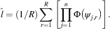(19) $$\hat{l}=\left( {{1 \mathord{\left/ {\vphantom {1 R}} \right. \kern-\nulldelimiterspace} R}} \right)\mathop{\sum}\limits_{r=1}^R {\left[ {\prod\limits_{j=1}^n {\Phi \left( {\psi _{{j,r}} } \right)} } \right]} .$$

One can then maximize this simulated likelihood by any standard optimization routine to estimate parameters and apply the standard maximum likelihood (ML) estimator for the variance covariance ( $${\minus}[H{\rm (}\hat{l})]^{{{\minus}1}} $$ ).Footnote ¹⁸ Like ML, STP-MSL is BANC: best (asymptotically efficient) asymptotically normal and consistent.

ESTIMATED SPATIAL/SPATIOTEMPORAL EFFECTS AND RESPONSE PATHS WITH CERTAINTY ESTIMATES

Properly estimating parameters like coefficients and their certainties is an essential start to valid inference, but the ultimate aim is to estimate and draw inferences regarding effects (ideally: causal ones), that is, outcome responses associated with (ideally: caused by) changes in explanatory factors or other counterfactual shocks. We estimate coefficients like ρ, ϕ and β for the purposes of estimating effects like ${\textstyle{{\Delta y_{i}^{{\!\asterisk}} } \over {\Delta x_{i} }}}$ , that is, effects of changes in some x _i on the latent variable, y _i* or, better, on the outcome probability, ${\textstyle{{\Delta p(y_{i} =1)} \over {\Delta x_{i} }}}$ .Footnote ¹⁹ Given interdependence, even these sorts of within-unit counterfactuals (effects of x _i on y _i) involve feedback from i through other units j back to i. The effect of economic development in Senegal on its own probability of internal conflict, for instance, includes the reverberating feedback from Senegal to its neighbors and back. In contexts involving interdependence, however, interest usually focuses on cross-unit feedback effects, like ${\textstyle{{\Delta y_{j}^{{\!\asterisk}} } \over {\Delta x_{i} }}}$ or ${\textstyle{{\Delta p(y_{j} =1)} \over {\Delta x_{i} }}}$ (the reverberating effects of Senegalese development across Sub-Saharan Africa).Footnote ²⁰ For interdependent binary outcomes, perhaps most interesting of all would be effects on outcome probabilities in some unit(s) i of hypothetical outcomes in other units, j (y _j=1 or y _j=0), which we denote $${\textstyle{{\Delta p({\bf y}_{i} =1)} \over {\Delta {\bf y}_{j} }}}$$ : the effect on the probability of a Senegalese civil war on internal conflict versus peace in Guinea-Bissau, for instance. In spatiotemporal contexts, finally, we will want to estimate the response paths and long-run-steady-state effects of all of these sorts of hypotheticals.

Because they involve spatial, temporal or spatiotemporal feedback dynamics, none of these substantive effects or response paths is simple to estimate. The feedback multipliers (I−ρ W−ϕ L)⁻¹ imply that these various spatiotemporal effects and responses involve (nonlinear) combinations of coefficients and variables, so we could not read effects directly from a table of coefficients even if we confined discussion to responses in latent variables, $\hat{y}^{{\!\asterisk}} $ , rather than to the probabilities of actual interest, ${\hskip 4pt\vskip -1pt \hat}{\bf { {\hskip -2.7pt} p}}$ . Since the latent-variable model is a spatial linear regression, estimated effects in terms of $\hat{y}^{{\!\asterisk}} $ and their certainties would derive exactly as in that case, which we have discussed elsewhere (Franzese and Hays Reference Franzese and Hays2004, Reference Franzese and Hays2007, Reference Franzese and Hays2008a, Reference Franzese and Hays2008b; Hays et al. 2010; Appendix IV).

Beron and Vijverberg (Reference Beron and Vijverberg2004) cover the effect of changes in x _i on the outcome probability in unit i. Simply applying the chain rule, the immediate effect, including all spatial feedback, is:Footnote ²¹

(20) $${{\partial p(y_{i} =1\!\mid\!{\bf X,W})} \over {\partial x_{i} }}=\phi _{{pdf}} \left( {{{\left[ {\left( {{\bf I}{\minus}\rho {\bf W}} \right)^{{{\minus}1}} {\bf X\bbeta }} \right]_{i} } \mathord{\left/ {\vphantom {{\left[ {\left( {{\bf I}{\minus}\rho {\bf W}} \right)^{{{\minus}1}} {\bf X\beta }} \right]_{i} } {\sigma _{{u_{i} }} }}} \right. \kern-\nulldelimiterspace} {\sigma _{{u_{i} }} }}} \right){{\left[ {\left( {{\bf I}{\minus}\rho {\bf W}} \right)_{{ii}}^{{{\minus}1}} \bbeta } \right]} \mathord{\left/ {\vphantom {{\left[ {\left( {{\bf I}{\minus}\rho {\bf W}} \right)_{{ii}}^{{{\minus}1}} \beta } \right]} {\sigma _{{u_{i} }} }}} \right. \kern-\nulldelimiterspace} {\sigma _{{u_{i} }} }},$$

where ϕ _pdf is the univariate standard-normal density function. This calculation can be extended straightforwardly to include steady-state effects and response paths as well as cross-unit effects.

We focus below on perhaps the most substantively interesting type of effect, which, to the best of our knowledge, has not been considered elsewhere: the response path in outcome probabilities for some unit(s) i from hypothetical changes to outcomes in other unit(s) j. We start with the response path in outcome probabilities for a single unit i to a change at time t in the outcome for a single unit j. Using the definition of conditional probability, these effects are calculated as:Footnote

(21) $$\eqalignno{ \qquad & p[y_{{i,t{\plus}s}} {\rm =}1\!\mid \!y_{{j,t}} {\rm =}1;{\bf X},{\bf W},{\bf L}]{\minus}p[y_{{i,t{\plus}s}} {\rm =}1\!\mid\!y_{{j,t}} {\rm =}0;{\bf X},{\bf W},{\bf L}] \cr =& {{p[y_{{i,t{\plus}s}} {\rm =}1,y_{{j,t}} {\rm =}1\!\mid\!{\bf X},{\bf W},{\bf L}]} \over {p[y_{{j,t}} {\rm =}1\!\mid\!{\bf X},{\bf W},{\bf L}]}}{\minus}{{p[y_{{i,t{\plus}s}} {\rm =}1,y_{{j,t}} {\rm =}0\!\mid\!{\bf X},{\bf W},{\bf L}]} \over {p[y_{{j,t}} {\rm =}0\!\mid\!{\bf X},{\bf W},{\bf L}]}},{\rm for }\ s{\rm =}0,\,\ldots\, .\qquad\qquad \ \\ \ (21)^{22}$$

Thus, given estimates of ρ, ϕ and β, we calculate the cumulative distribution functions for two univariate and two multivariate-normal distributions, one for each side of the counterfactual, to produce an estimated spatiotemporal response path (or spatial or spatiotemporal long-run steady-state effect).Footnote ²³ The joint probabilities in the numerators depend on the strength of the spatiotemporal connections between y _i,t+s and y _j,t. When s is small, the spatial connection largely determines the size of the effect. As s gets large, the time between events grows and p[y _i,t+s=1,0 $\mid $ y _j,t=1,0] converges to p[y _i,t+s=1,0]×p[y _j,t=1,0], driving the effect to 0. We estimate uncertainties for these estimated spatiotemporal responses by parametric simulation: repeat the procedure for each of many draws of parameter estimates from their estimated joint distribution, and the average and standard deviation across draws give the estimate and its standard error.Footnote ²⁴ For those who study interdependence in binary outcomes, these and related quantities are substantively important. In the Monte Carlo experiments and illustration that follow, we evaluate our ability to estimate this conditional effect accurately and then use this calculation for analytical purposes.

MONTE CARLO ANALYSES

We explore the small-sample properties of the STP-MSL estimator for the spatiotemporal-lag probit model using a data-generation process that follows as closely as possible Beron and Vijverberg’s (Reference Beron and Vijverberg2004) purely cross-sectional spatial-probit Monte Carlo experiments.Footnote ²⁵ We evaluate the quality of the STP-MSL parameter estimates, and of the spatial and spatiotemporal effect estimates described in the Estimated Spatial/Spatiotemporal Effects and Response Paths with Certainty Estimates section. Regarding the effect estimates, we compare the small-sample performance of our suggested strategy for calculating first differences in probabilities for y _i conditional on outcomes y _j≠i with effect estimates from naïve spatiotemporal-probit models that include spatial lags (but treat them as exogenous regressors) and that address temporal dynamics using either a first-order Markov regime-switching or discrete-time hazard framework. The former includes time-lagged observed outcome, Ly, not Ly*, as a regressor, and the latter a polynomial in time-since-event, s, (we use s, s ² and s ³). With all regressors assumed to be exogenous, both naïve models apply simple ML as the estimator. Our spatiotemporal data-generating process takes the form:

(22) $${\bf y}^{{\!\asterisk}}\! =\left( {{\bf I}_{n} {\minus}\rho {\bf W}{\minus}\phi {\bf L}} \right)^{{{\minus}1}} \left( {\beta _{0} {\plus}\beta _{1} {\bf x}{\plus}{\bf {\bvarepsilon}}} \right){\rm ,\ }{\bf {\bvarepsilon}}\:\sim\:N\left( {0,1} \right).$$

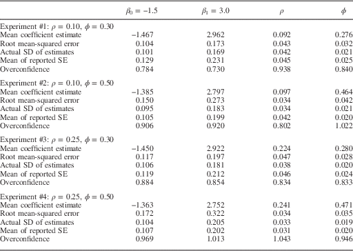
We apply Equation 3 to generate y from these y*. For W, we use a row-standardized binary-contiguity matrix with the 50 US states as in Beron and Vivjerberg (2004). Data for each unit are generated for 20 periods, giving us a sample size of 1,000 in each of our Monte Carlo experiments.Footnote ²⁶ In each of our experiments we set β ₀=−1.5, and β ₁=3.0, yet vary ρ={0.10, 0.25} and ϕ={0.30, 0.5}, giving us four experiments with different levels of spatial and temporal dependence. Finally, x is drawn from a standard uniform distribution on the interval [−1, 2], resulting in an expected value of 0.5 and a variance of roughly 2. These choices produce, on average, a balanced sample of 0’s and 1’s. Table 1 presents results for 100 trials using the STP-MSL-RIS spatiotemporal-probit estimator (with R=100).Footnote ²⁷ We do not compare these parameter estimates with those of the naïve spatiotemporal-probit, because the forms of temporal dependence they assume (regime-switching, discrete-time hazard) do not generate the same parameters as Equation 22. Comparing the implied first/same-period spatial effects is appropriate, though, and we do so below.

Table 1

Simulation Results for STP-MSL by RIS Parameter Estimates (100 Trials)

Note: N=50 and T=20 for all experiments reported in text.

We begin by noting that our estimates are reasonably accurate across all of the experiments. The mean coefficient estimates are always within 10 percent of the true parameter values. This performance compares favorably to the results in Beron and Vijverberg (Reference Beron and Vijverberg2004) and can be explained by our sample sizes, which are larger than theirs, as well as by the fact that the covariate, x, in our data-generating process has a larger variance. Despite this accuracy, our results exhibit the well-known small-sample bias in ML estimates of autoregressive-lag models: a tendency to underestimate, on average, both the spatial coefficient ρ as well as the time-dependence coefficient ϕ. The bias in the mean estimate for ρ seems to grow slightly in percentage terms as we increase its true value from 0.10 to 0.25, whereas the bias in the mean estimate for ϕ drops in percentage terms as we increase the degree of temporal dependence from 0.30 to 0.50. However, given the relatively small number of trials in our experiments and the small changes observed in the biases, we do not want to attach too much significance to these patterns. We also see attenuation biases in the mean estimates for β ₀ and β ₁. These biases are quite small when the degree of spatiotemporal dependence is low, approximately 2 percent, but increase to around 8–10 percent when both ϕ and ρ are large.

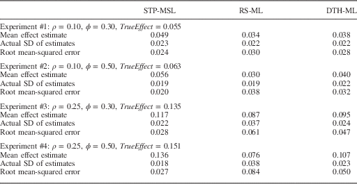
Ultimately, we are not interested in the parameter estimates per se, but rather in the effects that they imply. We start with the first difference $$\Pr [y_{i} =1\!\mid\!{\bf x},\,{\bf W},\,{\bf L},\,y_{j} =1]{\minus}\Pr [y_{i} =1\mid{\bf x},\,{\bf W},\,{\bf L},\,y_{j} =0]$$ for the immediate (first/same-period) spatial effect (that is, the effect of a time t change in the outcome for unit j on the time t probability that we observe a particular outcome for unit i). In Table 2, we compare the first/same-period spatial effect estimates implied by the spatiotemporal-lag model with comparable estimates from two naïve spatial models that address temporal dependence alternatively via regime switching (RS) or discrete-time hazard (DTH) functions. To illustrate, we select a specific pair of units i and j directly connected in the spatial-weights matrix (Alabama and Mississippi) and calculate the true effect, $$\Pr [y_{i} =1\!\mid\!{\bf x},\,{\bf W},\,{\bf L},\,y_{j} =1]{\minus}\Pr [y_{i} =1\!\mid\!{\bf x},\,{\bf W},\,{\bf L},\,y_{j} =0]$$ , assuming x equals its last sample values. In our example, the true effect size ranges from 0.055 to 0.151 given different levels of spatial and temporal dependence (as indicated in Table 2). To calculate these effects using the spatiotemporal-lag probit model, we use the parameter estimates noted above and the method outlined in the Estimated Spatial/Spatiotemporal Effects and Response Paths with Certainty Estimates section. The naïve spatial models replace the spatial-lag latent variable in Equation 22 with a spatial lag in observed outcomes, Wy, treating it as exogenous. The temporal-lag latent variable is replaced with a temporally lagged observed outcome in the RS model and with the last sample value of the peace years counter in the DTH model. To estimate the first/same-period spatial effect, we set y _j=0 and calculate Pr[y _i=1], change to y _j=1 and recalculate Pr[y _i=1], and then difference these probabilities.

Table 2

Simulation Results for Effect Estimates (100 Trials)

It is possible that the naïve alternatives do well enough in terms of effect estimates that they provide reasonable substitutes for the more complicated STP-MSL estimator, even when the spatiotemporal-lag probit model is the true data-generating process. In Table 2, we show that this is not the case. As noted in Table 1, STP-MSL slightly underestimates, on average, all of the model’s parameters. Consequently, it will also underestimate the first difference $$\Pr [y_{i} =1\!\mid\!{\bf x},\,{\bf W},\,{\bf L},\,y_{j} =1]{\minus}\Pr [y_{i} =1\!\mid\!{\bf x},\,{\bf W},\,{\bf L},\,y_{j} =0]$$ . Across the four experiments, the effect estimate by STP-MSL is ~89 percent of the true first difference. This compares with average effect estimates across the experiments of 68 and 56 percent for the DTH-ML and RS-ML models, respectively. In our experiments, the performance gap in terms of bias is largest when the degree of temporal dependence is high. This is true when performance is gauged in root-mean-square error (RMSE) terms as well. When ρ is 0.25 and ϕ is 0.5, the RMSE for the DTH-ML effect estimate is 85 percent larger than the STP-MSL estimator, and the RMSE for the RS-ML effect estimate is 211 percent larger. Thus, we do not find evidence to suggest that the simpler DTH-ML and RS-ML models provide reasonably approximate effect estimates when the spatiotemporal-lag probit is the true data-generating process.

Moreover, note that the consequences of the naïve models’ misspecifications, both assuming the spatial lag is exogenous and getting the temporal dynamics wrong, are minimized in these first/same-period spatial-effect estimates. Misspecifying temporal dynamics has relatively little impact on immediate-effect estimates, and the coefficient-estimate bias from assuming that the spatial-lag is exogenous arises in part because it accounts for both direct and indirect effects, both of which these spatial-effect estimates incorporate to some degree. Thus Table 2 represents the best case for the naïve spatial models. Most other effect estimates of interest would exhibit larger, likely much larger, performance gaps.

Figure 1 graphs the spatiotemporal response paths for these Monte Carlo experiments, using the spatially and temporally lagged latent variable probit model.Footnote ²⁸ The graph provides information about (1) the bias in our response-path estimates, comparing the truth triangles and average-estimate diamonds, (2) the efficiency of these estimates, by the 95-percentile range across trials in the estimates and (3) the accuracy of our uncertainty estimates, by the horizontal check marks giving the average 95 percent confidence interval estimates.Footnote ²⁹ As expected, these estimated response paths, which begin with the first/same-period spatial effects from Tables 1 and 2, decay over time, and we tend to slightly underestimate their magnitudes due to the underestimation of ρ and ϕ. Certainty estimates tend to be quite accurate as well, marginally under-confident in (many of) the first periods, and occasionally over-confident thereafter. In totality, the estimated response paths reflect the true paths accurately.

Fig. 1

Accuracy of STP-MSL estimates of spatiotemporal response-path estimates. Note: horizontal bars indicate 95 percent confidence intervals using the estimated standard errors (within trials); vertical lines indicate 95 percent intervals using the actual standard deviation of the effect estimates (across trials). ♦=estimated response paths; ▲=true response paths

ILLUSTRATION: CONTAGION OF CONFLICT IN AFRICA

To illustrate, we model the (inter)dependence in civil conflict episodes, estimating spatial and spatiotemporal-lag models of civil war incidences in Sub-Saharan Africa, covering all countries from 1966 to 2001.Footnote ³⁰ Anecdotally, signs of spatiotemporal dependence in the region’s civil conflict dynamics seem strong. Several countries in the Great Lakes region of (East) Africa (for example, DRC, Uganda, Rwanda, Burundi, Tanzania) have seen numerous civil wars that appear related. O’Loughlin and Raleigh (Reference Pinkse and Slade2008, 10) argue that these conflicts “highlight how many current civil wars are not state-specific, but related and supported by a host of external conditions.”Footnote ³¹ The West Africa region (for example, Sierra Leone, Liberia, Guinea, Senegal) seems to exhibit similar conflict dynamics. In 2003, The Economist reported: “West Africa’s civil wars are usually reported as tragedies befalling individual states…In fact, all these wars are intertwined, and it is impossible to understand one without reference to the others.” These accounts highlight the need to explicitly account for spatial interdependence in analyses of civil war.

Theoretically, conflict studies recognizing spatial dependence in civil wars are hardly new. A large and long-standing literature concludes that civil conflicts diffuse across international borders, with violence in one country making civil war more likely in adjacent ones (for example, Most and Starr Reference Murdoch and Sandler1980; Starr and Most Reference Starr and Most1983; Diehl Reference Diehl1991; Lake and Rothchild Reference LeSage1998; Gleditsch 2002; Ward and Gleditsch Reference Ward and Gledistch2002).Footnote ³² Refinements have attempted to discern and distinguish the specific mechanisms by which civil war diffusion occurs (Murdoch and Sandler 2002; Saleyhan and Gleditsch 2006; Buhaug and Gleditsch Reference Buhaug and Gleditsch2008), to understand the ability of some states to resist transmission (Raleigh Reference Salehyan and Gledistch2004; Braithwaite Reference Braithwaite2010) and to explore how expectations of diffusion may influence third-party intervention (Kathman Reference Klier and McMillen2010). This research has generally inferred support for such neighborhood effects from the significance of some spatial-parameter estimate, usually the coefficient on a spatial lag of conflict (occasionally, time-lagged spatial lag) entered in a standard logit or probit estimation. Usually the simultaneity of these spatial lags goes unaddressed, and the likely high levels of interdependence suggest the resultant biases may be substantial.Footnote ³³ Moreover, to our knowledge, no work has interpreted the effects of the estimated interdependence in terms of the spatial or spatiotemporal responses in civil conflict probabilities across countries to hypothetical shocks to civil conflict risks in some country or countries, as we suggest here.

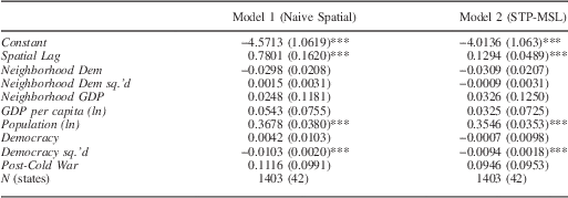
Therefore, we apply the STP-MSL estimator to a spatial-probit model of civil war incidence. In Models 1 and 2, we focus exclusively on (cross-sectional) spatial dependence, modeled by a simultaneous spatial lag (See Table 3). The spatial relationships between states are given by a row-standardized binary-contiguity W matrix, with the sample countries averaging 4.0167 neighbors (ranging from 1 to 8).Footnote ³⁴ Our data come from Buhaug and Gleditsch (Reference Buhaug and Gleditsch2008), who explore the extent to which regional conflict clustering stems from the spatial clustering of country-specific characteristics (that is, in X’s) rather than direct contagion or spillover of conflict. As they do, we measure conflict incidence using the UCDP/PRIO Armed Conflict Database, which codes civil conflicts as occurring if violent incidents between a state government and organized opposition result in at least 25 deaths.Footnote ³⁵ Our models include all of the regressors in Buhaug and Gleditsch’s full models, including measures for the most common predictors of civil war in peace studies (for example, GDP, Population, Regime Type).Footnote ³⁶

Though both models estimate a significant spatial-lag coefficient, the estimates from the naïve model would seem to radically overstate the extent of interdependence, as the estimate is nearly seven times what the STP-MSL estimates seem to indicate. However, as noted above, parameter estimates may belie the ability of either model to recover accurate estimates of spatial effects, which are of greater importance. That is, we are ultimately concerned about the extent to which neighboring conflict (peace) makes conflict more (less) likely in various interesting counterfactual questions we could pose regarding conflict spatial and/or spatiotemporal dynamics in Sub-Saharan Africa. Even just a cursory review of recent political coverage uncovers the tragic frequency with which such questions are (implicitly) posed: “Fears mount that Côte d’Ivoire conflict could spill to Liberia,”Footnote ³⁷ “Zambia Concerned About DRC conflict spillover,”Footnote ³⁸ “The conflict in Mali could be creating a ‘ticking time bomb’ for neighbouring Western Sahara,”Footnote ³⁹ etc. Such hypotheticals are examples of the conditional effects discussed in the Estimated Spatial/Spatiotemporal Effects and Response Paths with Certainty Estimates section. To illustrate how we can answer such substantively meaningful conditional probabilities, we explore the extent to which the outbreak of conflict in Guinea-Bissau in 1998 was a consequence of the ongoing conflict in neighboring Senegal, subject to the important caveat that we have not yet accounted for temporal dependence in conflict propensities.

Historically, the border between Guinea-Bissau and Senegal has been a breeding ground for instability. Guinea-Bissau served as the training ground for Mouvement des Forces Democratiques de Casamance (MFDC) fighters and a conduit to funnel arms into the decades-long Casamance conflict. Most view the 1998–99 civil war in Guinea-Bissau as an outgrowth of these same tensions, with Senegalese forces ultimately fighting on both sides of the conflict (Humphreys and Mohamed 2005).Footnote ⁴⁰ We explore the extent to which the conflict in Senegal affected the onset of civil war in Guinea-Bissau, or, stated differently to highlight the conditional probability of the counterfactual: in the absence of the Casamance conflict, how likely was conflict in Guinea-Bissau? Utilizing simulations as described in the Estimated Spatial/Spatiotemporal Effects and Response Paths with Certainty Estimates and Monte Carlo Analyses sections, Guinea-Bissau has a civil war 8.5 percent of the time when Senegal is peaceful and 11.14 percent of the time when Senegal is at war. Thus the model estimates suggest that Senegal’s conflict increased the risk of war in Guinea-Bissau by 2.64 percent. To calculate our uncertainty about these effects estimates, we sample parameter estimates from their estimated sampling distribution; doing so reveals that the effect sizes at the 5th and 95th percentiles are 0.90 and 4.89 percent, respectively.

Table 3

Spatial-Autoregressive Models of Conflict in Africa

Note: dependent variable: civil-war incidence (0=No, 1=Yes). All spatial lags use row-standardized binary-contiguity spatial-weights matrices. Significant at ***1, **5, *10%.

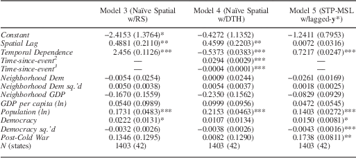
Next, using the time-series cross-section of these data, we estimate models accounting for both spatial and temporal dependence in conflict episodes (Table 4). The naïve model again appears to overstate the extent of spatial dependence, as both the RS-ML (Model 3) and DTH-ML (Model 4) models using an exogenous spatial lag indicate a significant spatial effect. When we estimate the spatiotemporal-lag probit model, however, we find a smaller and non-significant spatial-lag coefficient. What, then, causes the discrepancy between the insignificant spatial effect found here and the significant finding in all other models? We know that naïve estimation strategies (Models 3 and 4) that treat the spatial lag as exogenous will tend to overstate the degree of spatial dependence. Similarly, even if we account for the endogeneity of the spatial lag, failure to allow for the possibility of temporal dependence (Model 2) could lead us to infer incorrectly from our models that spatial dependence is present when it is not.Footnote ⁴¹

Table 4

Spatiotemporal Models of Conflict in Africa (Buhaug and Gleditsch Reference Buhaug and Gleditsch2008)

Note: dependent variable: civil-war incidence (0=No, 1=Yes). All spatial lags use row-standardized binary-contiguity spatial-weights matrices. Significant at ***1, **5, *10%.

This can be the case when the observable and unobservable determinants of an event cluster in both space and time, making it difficult for misspecified models to distinguish between spatial and temporal dependence. For example, if the level of democracy in Guinea-Bissau at time t−1 correlates with the level of democracy in Senegal at t−1 (spatial clustering)—which, in turn, correlates with the level of democracy in Senegal at time t (temporal clustering)—the latent propensity for civil war in Guinea-Bissau at time t−1 will correlate with the latent propensity for civil war in Senegal at time t. If there is only temporal dependence in the true data-generating process for a country’s latent propensity to experience civil war (and no spatial dependence), and we put Senegal’s latent propensity for civil war at time t on the right-hand side of Guinea-Bissau’s latent propensity at time t and exclude Guinea-Bissau’s latent propensity at time t−1, omitted-variable bias will erroneously make it seem as though there are spatial spillovers.Footnote ⁴²

This appears to be what we observe with respect to civil conflict. While we do not want to make sweeping claims on the basis of our admittedly limited illustration, we do want to emphasize that it is possible to mistake spatial dependence for temporal dependence and vice versa. Given that much of the scholarly quantitative literature finds spatial dependence in civil war and the popular press treats these spillovers as a nearly undeniable reality, this is important to know. Our analysis suggests that the evidence of such a relationship may not be as strong as currently believed.

We do, however, find that temporal dependence is, unsurprisingly, high and highly significant, indicating great persistence in conflict behavior. To analyze these temporal dynamics more explicitly, we again turn from estimated coefficients to estimated effects. Continuing with the Casamance conflict in Senegal as an example, but shifting focus to the temporal dynamics, this time we ask: What effect did Senegal’s prior conflict history have on the realization of conflict in 1998? In particular, beginning with 1992—when the conflict in Senegal escalated—we explore the extent to which fighting (or peace) from that point onward influenced the likelihood of conflict in 1998.

As before, we can use our simulation strategy to condition on a single counterfactual outcome, finding that conflict as opposed to peace in 1992 made Senegal 51.9 percent more likely to experience conflict in 1993.Footnote ⁴³ To estimate counterfactual response paths for various alternative conflict histories, we simply increase the number of outcomes that are conditioned upon (that is, the number of dimensions in our cumulative probability). Figure 2 illustrates, depicting six (of the possible 64) conflict histories since 1992 that could have preceded 1998 in Senegal. We compare each of these histories—lengths of sustained conflict since 1992 of 0 to 5 years—against one in which Senegal was peaceful for all those years, which is given by the thick-black x-axis.

Fig. 2

Estimated response-paths to alternative counterfactual conflict histories in Senegal

The results suggest some interesting features of conflict dynamics. First, the effects of conflict persistence (auto-dependence) are quite large immediately following a conflict, but dissipate rapidly once peace emerges. For instance, we estimate that, if the Senegalese conflict had ended after 1992, no discernible effect of previous conflict on future conflict probabilities would have persisted by 1998. (The thin solid line converges quickly to the steady state.) We also see how histories full of conflict can mire states in so-called conflict traps, as years of fighting produce high probabilities that conflict will persist into subsequent years. Notice, for instance, that at the end of the all-conflict counterfactual history, the likelihood of fighting in 1998 is 62 percent higher than it would be following the all-peace history.

Lastly, we compare the predictive accuracy of the spatiotemporal-lag probit model estimated by maximum simulated likelihood (STP-MSL), the regime-switching model estimated by maximum likelihood (RS-ML) and the discrete-time hazard model estimated by maximum likelihood (DTH-ML). We begin by focusing on the overall ability of the respective models to predict conflict and peace outcomes using the area under the receiver-operating characteristic (ROC) curve. In our illustration, ROC curves gauge the ability of each model to correctly predict instances of conflict or true positives without making false positive predictions across all possible prediction rules.Footnote ⁴⁴ Area under the curve (AUC) scores are portions of the area of the unit square and therefore range between 0 and 1, with higher scores indicating a better job of predicting peace and conflict outcomes. (A random model-free prediction strategy generates an AUC score of 0.5.) In terms of overall predictive performance, there is not much separation between the models. STP-MSL has the highest score (0.9318), but the difference in comparison with DTH-ML is minimal (0.9316). The performance gap with RS-ML is larger (0.9254), but remains minor.

In Figure 3, we divide the data into two sub-samples based on whether conflict was observed in the prior period, thereby allowing us to break down the ability of the models to accurately predict conflict onset (or peace duration) and conflict persistence (or peace onset). The AUC scores from the ROC curves indicate that DTH-ML (0.7342) and STP-MSL (0.7222) are more or less equivalent at predicting conflict onset (plot to the left in Figure 3), with DTH-ML offering a 1.7 percent improvement over STP-MSL and both besting RS-ML (0.6988). A clearer performance gap emerges when we focus on the prior conflict sub-sample (plot to the right in Figure 3), with STP-MSL outperforming both DTH-ML and RS-ML at most of the evaluated thresholds. Comparing AUC scores, STP-MSL (0.7090) offers a 9.6 percent improvement over RS-ML (0.6469) and a 4.2 percent improvement over DTH-ML (0.6801).

Fig. 3

ROC curves for onset and duration subsamples

In sum, STP-MSL has a slight advantage over DTH-ML and RS-ML in overall predictive performance. When we separate the data based on the prior outcome, we see that the superior performance of STP-MSL is due to its ability to better predict conflict duration (peace onset), with no estimator offering as clear an advantage in predicting conflict onset. While the predictive advantages offered by STP-MSL are relatively minor here, we expect that the benefits would be clearer in applications exhibiting significant spatial dependence.Footnote ⁴⁵ Furthermore, our unified autoregressive framework for spatial and temporal dependence is much more elegant than the alternatives. For this reason, and despite the added complexity surrounding parameter estimation, the spatiotemporal probit simplifies effect calculations both conceptually and computationally.