MOBILITY AND THE EVOLUTION OF PUBLIC SCHOOLS OVER THE TWENTIETH CENTURY

Current income mobility rates in the United States are similar to or below those of other countries. International comparisons of intergenerational income elasticities reveal that the correlation between a father's income and that of his son is stronger in the United States than in other developed nations.Footnote ¹ Historically, this has not been the case. Joseph Ferrie's study of intergenerational occupational mobility rates in the United States and Britain reveals that the United States had high levels of occupational mobility in the late 1800s. The mobility rates then converged over the first half of the twentieth century to the more modest international levels.Footnote ²

One key contribution to these changes may have been the evolution of the public education system. At the end of the nineteenth century, educational institutions in the United States bore little resemblance to the modern school system. The first decades of the twentieth century ushered in compulsory attendance laws, public funding of education, and the separation of grammar schools from high schools.Footnote ³ This transformation of American educational institutions led to dramatic increases in educational attainment and literacy rates.Footnote ⁴ It occurred at different times in different areas of the country, but the whole movement took place during the first half of the twentieth century.

The impact of the public school movement on income mobility can be ambiguous. Intuitively, the expansion of public schools should have created a more egalitarian school system and consequently greater mobility. Models of the transmission of earnings across generations in the tradition of Gary Becker's work on human capital and the family indeed predict an increase in intergenerational income mobility with a rise in government spending on education.Footnote ⁵ However, Arthur Goldberger notes that these results depend on an assumption that private and public education are substitutes.Footnote ⁶ If they are instead complements, it is possible that improvements in public schooling could lead to declines in intergenerational mobility. Therefore, identifying the effects of changes in educational institutions on intergenerational mobility is ultimately an empirical question.Footnote ⁷

Empirical work on the relationship between public schools and mobility has been limited by a lack of appropriate data. A small body of evidence suggests that additional government spending on education can lead to declining mobility. When access to higher education in Britain was expanded recently, wealthy families were able to take fuller advantage of the expanded opportunities.Footnote ⁸ Nathan Grawe demonstrates that for the United States in recent decades, states with larger average class sizes have higher rates of intergenerational mobility.Footnote ⁹ While Grawe's results concern the same public primary and secondary schools that are the focus of this study, his analysis is limited to school measures at the state level. The aggregation masks much of the heterogeneity in school characteristics. The Iowa data at the turn of the century used in this article afford an opportunity to consider variation in school characteristics at the district level. I will explore whether the negative relationship between public school quality and mobility identified by Grawe for the modern public school system was present in the early days of public school expansion when the data are disaggregated to the township level.

IOWA'S SCHOOL SYSTEM AT THE TURN OF THE CENTURY

The Iowa data are particularly valuable because Iowa offers the only opportunity in the early 1900s to create panel data across generations on income and schooling. Iowa was one of the first states to begin the transition to modern public graded schools and high schools. Between 1857 and 1870 Iowa increased the ability of townships to vote for the creation of schools and fund those schools through local taxes. The changes led to increased overall education expenditures and reduced the tuition burden on students. Between 1870 and 1900 the number of high schools in Iowa increased from 40 to over 200, appearing in the major cities but also in the towns and villages of the countryside.Footnote ¹⁰ In just the five years between 1895 and 1900, the number of graded schools increased by nearly 20 percent.Footnote ¹¹ In addition, there was a movement at the turn of the century toward school consolidation in the rural school districts, increasing the quality of education available to rural children. The result of all of these changes was a dramatic rise in both educational access and school quality between 1890 and 1910 that preceded much of the rest of the nation by two decades.Footnote ¹²

Iowa also led in the collection of school statistics on enrollment, teachers, expenditures, and revenues by school district in each year. The school district data can be combined with individual-level data from the 1915 Iowa state census, which asked for the number of years a person attended common school, grammar school, high school, and college. The 1915 Census also asked individuals for their annual earnings, making the census the only large survey containing both income and educational attainment data for the United States prior to the 1940 federal census.Footnote ¹³ By linking adult sons to their fathers in the Iowa census, an intergenerational data set can be generated containing two generations of income and educational attainment data. With a rapidly changing mix of schools, a wealth of school district data, and educational attainment and income data for the entire state population, the Iowa data offer a unique opportunity to study the relationship between education and intergenerational income mobility. While Iowa was an early mover in education, the changes there were mimicked later throughout the rest of the nation.

CONSTRUCTING AN INTERGENERATIONAL DATA SET

The Iowa census and schooling data are combined with evidence from the 1900 federal census to reconstruct the childhood households of the individuals surveyed in the 1915 Iowa census. The matching across censuses allows me to acquire the parental occupation and earnings data necessary for a study of intergenerational mobility. The construction of an intergenerational data set begins with the sample of the 1915 Iowa state census transcribed by Claudia Goldin and Lawrence Katz for their study on the returns to education.Footnote ¹⁴ They sample ten rural counties and the three counties with large urban populations (containing the cities of Davenport, Des Moines, and Dubuque). The resulting sample includes information for roughly 60,000 individuals on age, birthplace, parents' birthplaces, year of immigration, if applicable, years of schooling by school type (common, grammar, high school, college), occupation, months employed in the previous year, and annual earnings for the previous year.

From this sample of individuals, I select all males between the ages of 20 and 35 to constitute the sons of the father-son pairs in the final intergenerational data set. The age range is chosen such that the men are old enough to have moved out of their parents' household by 1915, but young enough that their fathers can still be located in the 1915 Iowa state census.

These young adult males are then located in the complete population schedules of the 1900 federal census, which is the only census in which the majority of the sons, aged 5 to 20 at the time of the census, will be living with their parents. Once a son is matched by the son's name, birthplace, and age to the federal census, information on his parents and siblings is transcribed from an image file of the original 1900 census form. Parents' birthplaces are recorded and used to confirm the accuracy of the match. Sibling information is used to determine the birth order of the individual. The father's name, age, birthplace, occupation, and parents' birthplaces are all recorded.

The father is then located in the 1915 Iowa state census by searching both the Goldin-Katz sample and the original census records available on microfilm at the Newberry Library in Chicago.Footnote ¹⁵ Name, age, birthplace, and parents' birthplaces provide the criteria for identifying correct matches. Once located in the 1915 Iowa census, the 1915 location, occupation, educational attainment, months employed, and annual earnings of the father are recorded.

TABLE 1

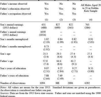
SUMMARY STATISTICS FOR THE FATHER-SON IOWA SAMPLE

Notes:

All values are means for the year 1915. Standard deviations are given in parentheses. An observation is considered one father-son pair.

Sources:

Data are from the 1915 Iowa state census. Father and sons are matched using the 1900 federal census.

The end result is a sample of father-son pairs with information for both father and son on occupation and earnings in 1915 and overall educational attainment. The father's occupation in 1900 is also known. The final sample is comparable in size to the modern panel studies for the United States used to estimate intergenerational income elasticities. The sample sizes are fairly large, ranging from 1,094 father-son pairs with complete income and occupation information to 3,488 pairs when including all observations for which there is at least an occupation for the father. The effects of the high school movement can be seen in the means for the sample in Table 1 by noting the jump in average educational attainment of over a year from the fathers' generation to the sons'. The lower earnings of the sons are attributable to the difference in average age between the sons and fathers.

While this sample of father-son pairs does have educational attainment data, it lacks information on educational access and quality, both of which are central to decisions about educational attainment and likely to be major factors in the extent to which education influences mobility. To incorporate these data into the father-son sample, the county superintendents of schools records from 1900 are transcribed and the sons are matched to their respective school districts based on their 1900 household locations. Some counties reported school district data at the township level, while others reported separate data for each subdistrict within a township. For rural individuals not living in a town, the subdistrict the individual lived in is not known so I aggregate the subdistrict data, if given in the superintendent records, together into a single township-level district. For individuals located in a rural township but living in a town, I match the person to the district data for their town rather than relying on township-level data. For urban individuals, I cannot determine their location within their township and must take the approach of constructing an aggregate township-level district. Incorporating the county superintendent data adds information on the availability of schooling types, local education expenditures, school district taxes, tuition levels, costs of books, teacher quality, and curriculum to the father-son pairs.

The data present several options for measuring intergenerational mobility: occupational transitions, geographical mobility, and income mobility. My focus will be on income mobility. Given ideal data, one would obtain the intergenerational income elasticity by simply regressing son's permanent log income on father's permanent log income, with the coefficient on father's permanent log income being the intergenerational income elasticity. A larger value for this elasticity indicates less income mobility. Unfortunately, I have data on annual income but not permanent income. Annual income varies from year to year because of both random, transitory shocks and systematic changes in income over the life cycle. Both sources of variation make any single observation of annual income a poor proxy of average annual income over the lifetime of the individual. The measurement error introduced by using annual income in a specific year as a proxy for permanent income will bias estimates of the intergenerational income elasticity downward and overstate the degree of intergenerational mobility observed.

The contribution of age-specific changes in income is controlled for through the inclusion of polynomials in sons' and fathers' ages. The regressions must also account for differences in the shape of the lifetime earnings profile for low- and high-income individuals. The steeper earnings trajectory early in life of high lifetime earnings individuals relative to low lifetime earnings individuals leads to different estimates of intergenerational income elasticities depending on the age at which individuals are observed.Footnote ¹⁶ To control for the divergence of earnings over the life cycle, I follow the approach of Gary Solon and Chul-In Lee and interact son's age with father's income, allowing the intergenerational income elasticity to vary the with son's age.Footnote ¹⁷ Incorporating these age controls and interaction terms, the equation used to estimate the intergenerational income elasticity is given by

(1)

where y_i,s and y_i,f are the son's and father's respective annual incomes and A_i,s and A_i,f are the son's and father's respective ages. By defining A_i,s to be son's age at the time of the income observation minus 30, Γ₁ can be interpreted as the intergenerational income elasticity for an individual at the age of 30, a measure comparable to the elasticities estimated in modern studies.

The transitory fluctuations in income present a less tractable problem. The standard approach to minimizing the bias introduced by these fluctuations is to average several observations of log annual income, a luxury not afforded by the Iowa data. This inability to average over several periods makes the measurement error more severe and the downward bias on the intergenerational income elasticity estimate greater than in modern studies. While there is no way to fully correct for this bias, I will provide modern intergenerational income elasticities measured both using single income observations and income averaged over several periods to provide a sense of the size of the bias.Footnote ¹⁸

TABLE 2

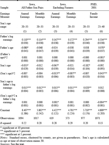
INTERGENERATIONAL INCOME ELASTICITY ESTIMATES FOR THE IOWA SAMPLE, SON's LOG EARNINGS AS DEPENDENT VARIABLE

* significant at 10 percent.

** significant at 5 percent.

*** significant at 1 percent.

Notes:

Standard errors, clustered by county, are given in parentheses. Son's age is calculated as age at time of observation minus 30.

Sources:

See the text.

INTERGENERATIONAL INCOME MOBILITY AT THE TURN OF THE CENTURY

Table 2 presents the intergenerational income elasticity estimates using the 1915 Iowa father-son pairs using both annual earnings and monthly earnings, defined as annual earnings divided by months employed. While annual earnings provide a better measure of overall welfare, the average monthly earnings may offer a clearer picture of the differences in the wage rates of fathers and sons. Both earnings measures produce similar estimates of 0.11 for the intergenerational income elasticity, suggesting that a 10 percent increase in father's earnings leads to a roughly one percent increase in predicted earnings for a son of age 30.

The Iowa elasticity of 0.11 is substantially below the 0.3 to 0.5 range of elasticities estimated by Tom Hertz and Solon and Lee.Footnote ¹⁹ Even when using a single observation of income, and therefore producing an attenuation bias similar to the bias affecting our results, Solon gets estimates of the modern intergenerational income elasticity ranging between 0.29 and 0.41, still substantially larger than the Iowa estimates.Footnote ²⁰ Some of the differences between the early Iowa elasticities and the modern ones might arise due to differences in specification and other factors. As a robustness check, I estimated elasticities for the modern era using the specification used for the early Iowa estimations as the specification for estimation using modern data from the 2001 Panel Study of Income Dynamics. The elasticities in columns 5 and 6 of Table 2 range from 0.29 to 0.33 and they are similar to the elasticities in the other modern studies.Footnote ²¹

While the intergenerational income elasticity for Iowa in 1915 is quite small by modern standards, there is a question of whether it truly signifies high rates of intergenerational mobility for early twentieth-century America or whether it is instead a product of the large proportion of the Iowa sample made up of farmers. As a group, farmers earned a wide range of annual incomes in the 1915 Iowa census, as farmers represented many of the poorest and richest individuals in the sample. This variability likely extends beyond differences across individuals to differences over time for any given individual, because farm output and crop prices fluctuated from year to year. All of this variation decreases the precision of annual earnings as a proxy for lifetime earnings, leading to lower intergenerational income elasticity estimates. Therefore, I estimate the elasticities for the Iowa sample excluding farmers. In columns 3 and 4 of Table 2, the results reveal that the large share of farming fathers and sons leads to lower intergenerational income elasticity estimates. However, the intergenerational income elasticity for nonfarmers in 1915 of 0.17 for a 30-year-old was still well below that of modern individuals, strengthening the conclusion that there was a substantial degree of income mobility in early-twentieth-century America.

A lingering sample composition concern regards migration out of state, a potentially significant issue considering the high levels of geographical mobility at the time.Footnote ²² Since the Iowa census is the source of income, sons who moved out of the state are never included in the data set, making the regression sample overrepresentative of stationary individuals. Individuals who left likely exhibited different income mobility patterns than those who stayed, but the direction of bias for intergenerational income elasticity estimates is uncertain. In the sample, sons who moved over long distances had higher mean incomes and educational attainments and lower levels of unemployment relative to sons that remained in the same township between 1900 and 1915.Footnote ²³ These differences in observable characteristics suggest that including sons who move out of state, if possible, could lead to different intergenerational income elasticity estimates.

SCHOOL ACCESS, SCHOOL QUALITY, AND MOBILITY

The Iowa data confirm that income mobility rates were quite high at the turn of the century compared to modern benchmarks. The question that remains is how the evolving public education system influenced these mobility rates. The inclusion of a measure of school quality interacted with father's log income in equation 1 offers a means of assessing whether the evolution of the public school system altered mobility patterns in Iowa by testing whether intergenerational income elasticities varied across school districts of differing quality.

The inclusion of school quality transforms the regression equation into

(2)

where Sⁱ is a measure of the school quality in the school district of father-son pairi in 1900. The coefficient γ⁸ on Sⁱ allows for a shift in income for all sons with a change in school quality. The coefficient Γ⁹ represents the marginal change in the intergenerational income elasticity resulting from an increase in school quality. A positive value for Γ⁹ would indicate that an increase in school quality is associated with an increase in the intergenerational income elasticity and thus a decline in income mobility.

A crucial assumption underlying this approach is that location choices, both in terms of where families located and where schools were built, were exogenous.Footnote ²⁴ If families relocated based on school quality or if school location was a product of variation in communities' tastes for public education, the school quality variable will be correlated with preferences for education, home environment, and other unobserved characteristics relevant to a son's earnings. Ruling out the endogeneity of location decisions is quite difficult. The means and various percentiles of the earnings distribution are remarkably similar across townships of differing levels of school access and quality measured in 1900.Footnote ²⁵ The similarity of the earnings distributions across school districts of different qualities and access suggests that schools were not being built with a higher frequency in wealthier districts and that there was no net migration of higher-income families, those most capable of moving, toward better school districts.

An additional concern about geographic mobility is that individuals raised in good school districts were more or less likely to move out of their districts after completing their education, raising the possibility that the probability of an individual dropping out of the intergenerational sample could be correlated with school district characteristics. To determine whether this is a major problem, I construct a sample of individuals in the same birth cohort as the sons in the intergenerational sample living in the sample counties in 1900 matched to their location in 1920 using the federal census.Footnote ²⁶ This allows me to estimate the percentage of individuals who moved out of Iowa conditional on childhood school district characteristics. The correlation between the number of graded classrooms per square mile and a dummy variable equal to one if an individual remained in a sample county was −0.09 while the correlation between spending per student and the dummy variable was only −0.01. The low correlations suggest that the probability of moving out of the sample is only weakly correlated with school district characteristics and is not a major concern.

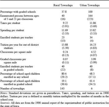
The detail of the county superintendent records allows me to examine the impacts on intergenerational mobility of geographical access to schools and of the quality of those schools. Geographical access is measured by the number of classrooms per square mile and the number of graded classrooms per square mile. School quality is measured by the teacher-student ratio, total expenditures per student, and taxes per student. The summary statistics of these measures and other school district characteristics in Table 3 show that urban areas had substantially higher values for the access measures and higher values for the school quality measures with the exception of teachers per enrolled student and the percentage of school-age children in any school. Equation 2 is estimated multiple times with a single schooling measure each time. This is done because multicollinearity problems arise when including multiple schooling measures that are highly correlated with one another. More importantly, the goal is to capture the effect of a general increase in school quality, not an increase in one dimension of school quality while all other dimensions are held constant.

TABLE 3

MEANS OF SCHOOLING MEASURES FOR RURAL AND URBAN SCHOOL DISTRICTS, 1900

Notes:

Standard deviations are given in parentheses. Taxes, spending, and tuition are in 1900 dollars. Tuition per year is defined as monthly tuition multiplied by the number of months in the school year.

Sources:

All data are from the 1900 annual report of the superintendent of public instruction for the state of Iowa.

To avoid the possibility that differences in income mobility measured in the regressions are driven by differences between rural and urban labor markets or rural-urban differences in unobserved school characteristics such as curricula, I estimate equation 2 for one subsample of individuals living in urban townships and another subsample of individuals living in rural townships.Footnote ²⁷ The subsample of individuals from rural townships is further divided into those living in towns and those living in the open country. The reason for dividing the sample in this way is that school characteristics have very different interpretations for the three different groups. All urban individuals have access to graded schools in their district; larger numbers of graded classrooms for urban individuals do not necessarily mean improved geographical access, but rather that students are attending larger schools or have multiple graded schools within the district. For individuals from rural townships living within towns, the presence of a graded school or more spending at that graded school speaks directly to the educational resources available to those individuals. For individuals living outside of towns, the importance of the presence of a graded school in their township and the quality of that graded school is mitigated by the fact that the school may have been costly to attend both in terms of travel time and tuition charged to out-of-district students. Towns with high schools typically had a district that was independent of the township-wide school district responsible for educating people in the open country. This is quite important given that all of the individuals in the sample would have attended school prior to the 1911 passage of Iowa's free tuition law, which gave every child a right to attend a high school free of charge even if they did not have a high school in their district. The law dramatically changed the schooling prospects of individuals going to high school in the years immediately following the cohorts in this study.Footnote ²⁸ These tuition costs are particularly relevant to this study as they were likely to have been a more severe constraint for poor families than for wealthy families. An improvement in geographical access to new high schools benefitted wealthy families, but not poor families if tuition costs were large enough that only wealthy families could afford to attend. In such a situation, the presence of a high school would have led to lower intergenerational mobility.

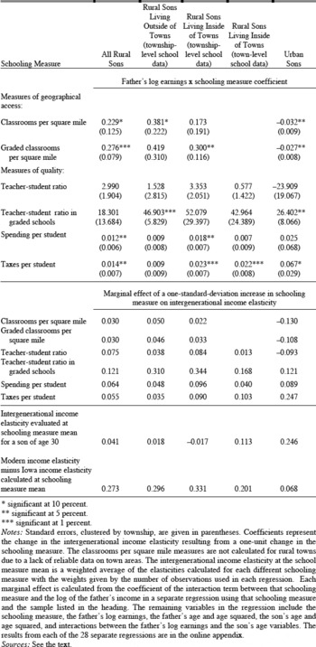
The estimated coefficients for the interaction term for schooling and father's log income from regressions for each schooling measure and each group are summarized in Table 4.Footnote ²⁹ For the rural townships, all of the coefficients are positive and consistent with improvements in school districts being associated with declines in income mobility. The positive coefficients on both the density of all classrooms and density of graded classrooms in a township suggest that improving geographical access to schools increased the intergenerational income elasticity, reducing mobility. A one-standard-deviation increase in graded schools per square mile is associated with a 3 percentage point increase in the intergenerational income elasticity for a 30-year-old son. The change of 0.03 accounts for roughly one-sixth of the difference between the intergenerational income elasticity of 0.11 for Iowa in 1915 and the 0.294 elasticity from the PSID data for 2001 in Table 2. The elasticities for the school quality measures for individuals in rural townships provide a similar picture. Increases in either spending per student or in taxes per student are associated with increases in the intergenerational income elasticity. As with the access measures, these coefficients are quite large. A one-standard-deviation change in spending per student for a rural township is associated with a 6 percentage point increase in the intergenerational income elasticity for a 30-year-old son. The positive coefficients for the teacher-student ratio measures suggest that improvements in quality measured by a reduction in the number of students per teacher were also associated with increases in the intergenerational income elasticity.

TABLE 4

MARGINAL EFFECTS OF SCHOOL QUALITY AND ACCESS ON THE INTERGENERATIONAL INCOME ELASTICITY

* significant at 10 percent.

** significant at 5 percent.

*** significant at 1 percent.

Notes:

Standard errors, clustered by township, are given in parentheses. Coefficients represent the change in the intergenerational income elasticity resulting from a one-unit change in the schooling measure. The classrooms per square mile measures are not calculated for rural towns due to a lack of reliable data on town areas. The intergenerational income elasticity at the school measure mean is a weighted average of the elasticities calculated for each different schooling measure with the weights given by the number of observations used in each regression. Each marginal effect is calculated from the coefficient of the interaction term between that schooling measure and the log of the father's income in a separate regression using that schooling measure and the sample listed in the heading. The remaining variables in the regression include the schooling measure, the father's log earnings, the father's age and age squared, the son's age and age squared, and interactions between the father's log earnings and the son's age variables. The results from each of the 28 separate regressions are in the online appendix.

Sources:

See the text.

The urban estimates offer mixed results. As with rural townships, spending per student and taxes per student have large, positive coefficients suggesting that increases in urban school district quality reduced mobility although the coefficients are not highly statistically significant. Increases in the teacher-student ratio in graded classrooms were associated with a statistically significant decrease in income mobility. The pattern reverses for the access measures, with both classrooms per square mile and graded classrooms per square mile having statistically significant, negative coefficients. However, given the large number of graded classrooms in urban townships, these variables can no longer be considered indicators of meaningful differences in geographical access to schools. Instead, they are far more complicated measures, capturing information on the extent to which children are sorted between multiple classrooms and schools within a district. A possible explanation for the negative sign on the urban classroom density coefficients comes from the results presented later in the article that wealthy families were more responsive to improvements in school access. If several graded classrooms already existed in these urban districts, wealthy students were already attending school. The marginal student would have been a poor student. Adding more classrooms would therefore have a larger impact on poor students in these urban districts, increasing income mobility.

The results suggest that in the first stages of the expansion of graded schools and high schools, captured by the experience of the rural individuals in our sample, intergenerational income elasticities were higher in townships with better school access and quality. The urban township results suggest that this negative association between school access and mobility may have been specific to the early days of school expansion when few graded schools and high schools existed. Once these schools became reasonably common and geographical access was no longer a primary issue, as in the case of the urban townships in the Iowa sample, this negative relationship is reversed.

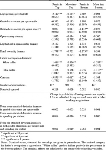
Table 5 presents full results from four regressions that offer an alternative way to examine the effects of schooling improvements on mobility by focusing on the tails of the income distribution. Following the approach of Richard Steckel and Jayanthi Krishnan, I estimate logit regressions for individuals persisting in or moving into the bottom quintile of the income distribution.Footnote ³⁰ The dependent variable for the regression for persistence in the bottom is an indicator variable taking on a value of one for all observations when both the son and father were in the bottom income quintile and zero when the father was in the bottom quintile but the son was not. The dependent variable for the movement into the bottom quintile regression takes on a value of one when a father was not in the bottom quintile but the son was and a value of zero when both the father and son were not in the bottom quintile. Similar regressions are run for persistence in or movement into the top quintile. The independent variables include measures of both geographical access to schools, proxied by graded classrooms per square mile, school quality, proxied by spending per student, and school tuition if the individual lives in the open country. School tuition is interacted with the open country dummy because the tuition is only being charged to out-of-district students, who were typically those students living in the open country. The tuition was not relevant to in-district students as they could attend for free even prior to the free tuition law. The regressions include controls for the initial conditions of the son including the type of area he lived in and his father's occupational category.

TABLE 5

LOGIT REGRESSION COEFFICIENTS FOR PERSISTENCE IN AND MOVEMENT INTO TOP AND BOTTOM EARNINGS QUINTILES

* significant at 10 percent.

** significant at 5 percent.

*** significant at 1 percent.

Notes:

Standard errors, clustered by township, are given in parentheses. The omitted category for father's occupation is agriculture. “White collar” predicts failure perfectly for persistence in the bottom quintile. The marginal effects are calculated at the mean of the schooling variables.

The most prominent result from the logit regressions is that improvements in schools significantly increased the rigidity in the tails of the income distribution. A one-standard-deviation increase in spending per student and graded classrooms per square mile was associated with a 5 percentage point increase in the probability of persisting in the top income quintile. There was a similarly large effect of school improvements on persistence in the bottom quintile. A one-standard-deviation increase in spending per student and graded classrooms per square mile was associated with a 6 percentage point increase in the probability of remaining in the bottom income quintile. Improvements in both school access and quality were associated with decreases in the likelihood of a son moving into the top income quintile, but had no statistically significant impact on the likelihood of a son moving into the bottom quintile. These findings of increased persistence in the tails of the income distribution with schooling improvements reinforce the negative relationship between schooling resources and mobility from the intergenerational income elasticity estimates.

SCHOOL EXPANSION AND EDUCATIONAL ATTAINMENT DECISIONS

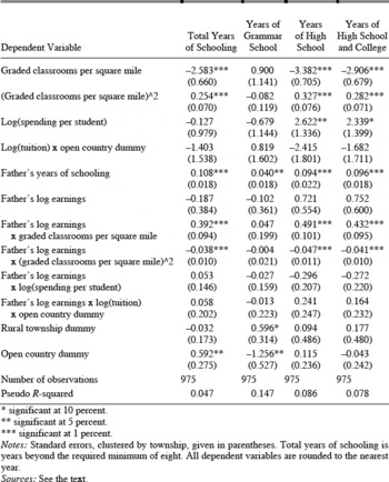
The results from both the income elasticity and logit regressions suggest that the presence of better public schools affected high income and poor families differently. The most likely source of these differences in mobility were differential responses across the income distribution in terms of educational investments and the returns to those investments; therefore, I estimate an ordered probit model with years of schooling as the dependent variable. Years of schooling are assumed to be a function of parental income, parental education, local school quality measured as spending per student, local school access measured as the number of graded classrooms per square mile, school tuition costs for those individuals living in the open country, and whether the family lives in an urban area, a town or in the open country.Footnote ³¹ Including interactions between parental income and the school access and quality variables allows the response to a change in local schools to vary across the income distribution. Positive coefficients on these interaction terms would indicate that higher income families' schooling investments responded more strongly to school access and quality, a finding that offers an explanation for the lower mobility levels in communities with better schools. An interaction between parental income and tuition is included to account for the possibility that tuition represented a larger burden for poorer families and thus reduced the number of years of school they attended.

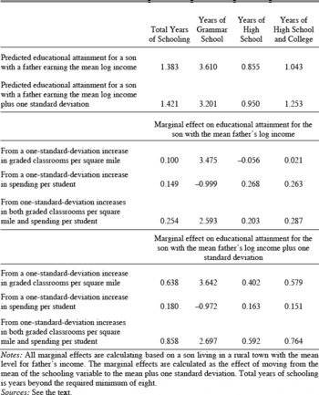
Coefficients for the probit estimates are given in Table 6. Table 7 compares the changes in the predicted level of education resulting from a one-standard-deviation increase in school access (and in school quality) for a son with a father having the mean log income with changes for a son whose father's income was one standard deviation above the mean. One-standard-deviation increases in both school access and school quality led to increases in overall educational attainment of every type for both a son from an average income family and a son from a high-income family.Footnote ³² The magnitudes of these increases are substantial. Predicted years of high school and college at the means of the schooling measures start at one year when the father's log income is at the mean and start at 1.25 years when a father's log income is one standard deviation above the mean. The predicted increases in high school and college attainment on the order of half a year when spending and access are both increased by one standard deviation are therefore quite substantial. These figures underscore the fact that improvements in schooling led to substantial absolute gains throughout the income distribution.

While both a son from an average-income family and a son from a high-income family have large predicted increases in educational attainment with improvements in access and quality, the increase is substantially larger for a son from a high-income family. A son with a father earning the mean log income has an increase in years of high school and college attainment of 0.3 years when increasing school spending and access by one standard deviation. While this is an impressive absolute gain, the predicted increase in high school and college attainment for a son from a high-income family of 0.8 years is over twice as large. These larger gains in educational attainment for the son from the high-income family are driven primarily by the response to improved access, captured by the large, positive coefficient on the interaction term between father's log income and school access in Table 6. While a one-standard-deviation increase in graded schools per square mile has a large effect on the educational attainment of a son from a high-income family, it has far smaller effects on the son from an average-income family. A one-standard-deviation increase in school quality has far more similar effects on the two sons and actually favors the son from the average-income family in the case of high school and college attainment, but these differences are quite small relative to the differences driven by changing access.

TABLE 6

ORDERED PROBIT REGRESSION COEFFICIENTS, SON's EDUCATIONAL ATTAINMENT AS DEPENDENT VARIABLE

* significant at 10 percent.

** significant at 5 percent.

*** significant at 1 percent.

Notes:

Standard errors, clustered by township, given in parentheses. Total years of schooling is years beyond the required minimum of eight. All dependent variables are rounded to the nearest year.

Sources:

See the text.

TABLE 7

PREDICTED YEARS OF EDUCATIONAL ATTAINMENT AND THE MARGINAL EFFECTS OF INCREASES IN SCHOOL QUALITY AND ACCESS ON SON's EDUCATIONAL ATTAINMENT BASED ON ORDERED PROBIT REGRESSION RESULTS

Notes:

All marginal effects are calculating based on a son living in a rural town with the mean level for father's income. The marginal effects are calculated as the effect of moving from the mean of the schooling variable to the mean plus one standard deviation. Total years of schooling is years beyond the required minimum of eight.

Sources:

See the text.

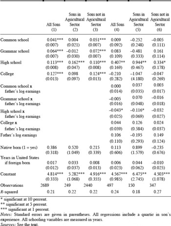
These probit results suggest that improving school access was leading to large increases in educational attainment across the income distribution, but that those increases were larger for sons from higher income families. To understand how these differences in educational attainment translated into differences in sons' incomes, Table 8 presents regressions of son's log income on years of education controlling for father's income and other characteristics. The results suggest that the high returns to education found by Goldin and Katz differed very little with respect to the father's income.Footnote ³³ In fact, the only statistically significant case in which returns to schooling differ by father's income is the returns to high school attainment where the negative coefficient on the interaction between high school attainment and father's earnings indicates that individuals from poorer families actually experienced higher returns to high school. Furthermore, unlike in the intergenerational income elasticity regressions, father's income is no longer statistically significant. This reinforces the idea that the decreases in mobility associated with greater school access and quality were being driven by the differences in educational investment decisions across the income distribution. The large returns to education shown in Table 8 reveal that these differences in educational attainment translated into large differences in income. Given the coefficients on high school and college, the additional half a year increase in high school and college attainment for a child from a high-income family relative to a child from an average-income family would translate into roughly an additional 5 percent increase in annual earnings for the child from the high-income family relative to the child from the average income family.