


%20--%3e%3c!DOCTYPE%20svg%20PUBLIC%20'-//W3C//DTD%20SVG%201.0//EN'%20'http://www.w3.org/TR/2001/REC-SVG-20010904/DTD/svg10.dtd'%3e%3csvg%20version='1.0'%20id='Layer_1'%20xmlns='http://www.w3.org/2000/svg'%20xmlns:xlink='http://www.w3.org/1999/xlink'%20x='0px'%20y='0px'%20width='64px'%20height='64px'%20viewBox='5.5%20-3.5%2064%2064'%20enable-background='new%205.5%20-3.5%2064%2064'%20xml:space='preserve'%3e%3cg%3e%3ccircle%20fill='%23FFFFFF'%20fill-opacity='0'%20cx='37.785'%20cy='28.501'%20r='28.836'/%3e%3cpath%20fill='%23595959'%20d='M37.441-3.5c8.951,0,16.572,3.125,22.857,9.372c3.008,3.009,5.295,6.448,6.857,10.314%20c1.561,3.867,2.344,7.971,2.344,12.314c0,4.381-0.773,8.486-2.314,12.313c-1.543,3.828-3.82,7.21-6.828,10.143%20c-3.123,3.085-6.666,5.448-10.629,7.086c-3.961,1.638-8.057,2.457-12.285,2.457s-8.276-0.808-12.143-2.429%20c-3.866-1.618-7.333-3.961-10.4-7.027c-3.067-3.066-5.4-6.524-7-10.372S5.5,32.767,5.5,28.5c0-4.229,0.809-8.295,2.428-12.2%20c1.619-3.905,3.972-7.4,7.057-10.486C21.08-0.394,28.565-3.5,37.441-3.5z%20M37.557,2.272c-7.314,0-13.467,2.553-18.458,7.657%20c-2.515,2.553-4.448,5.419-5.8,8.6c-1.354,3.181-2.029,6.505-2.029,9.972c0,3.429,0.675,6.734,2.029,9.913%20c1.353,3.183,3.285,6.021,5.8,8.516c2.514,2.496,5.351,4.399,8.515,5.715c3.161,1.314,6.476,1.971,9.943,1.971%20c3.428,0,6.75-0.665,9.973-1.999c3.219-1.335,6.121-3.257,8.713-5.771c4.99-4.876,7.484-10.99,7.484-18.344%20c0-3.543-0.648-6.895-1.943-10.057c-1.293-3.162-3.18-5.98-5.654-8.458C50.984,4.844,44.795,2.272,37.557,2.272z%20M37.156,23.187%20l-4.287,2.229c-0.458-0.951-1.019-1.619-1.685-2c-0.667-0.38-1.286-0.571-1.858-0.571c-2.856,0-4.286,1.885-4.286,5.657%20c0,1.714,0.362,3.084,1.085,4.113c0.724,1.029,1.791,1.544,3.201,1.544c1.867,0,3.181-0.915,3.944-2.743l3.942,2%20c-0.838,1.563-2,2.791-3.486,3.686c-1.484,0.896-3.123,1.343-4.914,1.343c-2.857,0-5.163-0.875-6.915-2.629%20c-1.752-1.752-2.628-4.19-2.628-7.313c0-3.048,0.886-5.466,2.657-7.257c1.771-1.79,4.009-2.686,6.715-2.686%20C32.604,18.558,35.441,20.101,37.156,23.187z%20M55.613,23.187l-4.229,2.229c-0.457-0.951-1.02-1.619-1.686-2%20c-0.668-0.38-1.307-0.571-1.914-0.571c-2.857,0-4.287,1.885-4.287,5.657c0,1.714,0.363,3.084,1.086,4.113%20c0.723,1.029,1.789,1.544,3.201,1.544c1.865,0,3.18-0.915,3.941-2.743l4,2c-0.875,1.563-2.057,2.791-3.541,3.686%20c-1.486,0.896-3.105,1.343-4.857,1.343c-2.896,0-5.209-0.875-6.941-2.629c-1.736-1.752-2.602-4.19-2.602-7.313%20c0-3.048,0.885-5.466,2.658-7.257c1.77-1.79,4.008-2.686,6.713-2.686C51.117,18.558,53.938,20.101,55.613,23.187z'/%3e%3c/g%3e%3c/svg%3e)
%20--%3e%3c!DOCTYPE%20svg%20PUBLIC%20'-//W3C//DTD%20SVG%201.0//EN'%20'http://www.w3.org/TR/2001/REC-SVG-20010904/DTD/svg10.dtd'%3e%3csvg%20version='1.0'%20id='Layer_1'%20xmlns='http://www.w3.org/2000/svg'%20xmlns:xlink='http://www.w3.org/1999/xlink'%20x='0px'%20y='0px'%20width='64px'%20height='64px'%20viewBox='5.5%20-3.5%2064%2064'%20enable-background='new%205.5%20-3.5%2064%2064'%20xml:space='preserve'%3e%3cg%3e%3ccircle%20fill='%23FFFFFF'%20fill-opacity='0'%20cx='37.637'%20cy='28.806'%20r='28.276'/%3e%3cg%3e%3cpath%20fill='%23595959'%20d='M37.443-3.5c8.988,0,16.57,3.085,22.742,9.257C66.393,11.967,69.5,19.548,69.5,28.5c0,8.991-3.049,16.476-9.145,22.456%20C53.879,57.319,46.242,60.5,37.443,60.5c-8.649,0-16.153-3.144-22.514-9.43C8.644,44.784,5.5,37.262,5.5,28.5%20c0-8.761,3.144-16.342,9.429-22.742C21.101-0.415,28.604-3.5,37.443-3.5z%20M37.557,2.272c-7.276,0-13.428,2.553-18.457,7.657%20c-5.22,5.334-7.829,11.525-7.829,18.572c0,7.086,2.59,13.22,7.77,18.398c5.181,5.182,11.352,7.771,18.514,7.771%20c7.123,0,13.334-2.607,18.629-7.828c5.029-4.838,7.543-10.952,7.543-18.343c0-7.276-2.553-13.465-7.656-18.571%20C50.967,4.824,44.795,2.272,37.557,2.272z%20M46.129,20.557v13.085h-3.656v15.542h-9.944V33.643h-3.656V20.557%20c0-0.572,0.2-1.057,0.599-1.457c0.401-0.399,0.887-0.6,1.457-0.6h13.144c0.533,0,1.01,0.2,1.428,0.6%20C45.918,19.5,46.129,19.986,46.129,20.557z%20M33.042,12.329c0-3.008,1.485-4.514,4.458-4.514s4.457,1.504,4.457,4.514%20c0,2.971-1.486,4.457-4.457,4.457S33.042,15.3,33.042,12.329z'/%3e%3c/g%3e%3c/g%3e%3c/svg%3e)
1. Introduction
There is a massive Black Hole (MB) at the Galactic Center (e.g., EHT 2022). It is believed that the MBH is surrounded by stars and compact objects, although only a few dozen of stars have been observed. The observed stars are called as S stars. S stars are orbiting the black hole along their Kepler orbits. From the magnitude of observed precession of S2, the mass of MBH and the enclosed mass within S2’s apocenter are estimated (GRAVITY Collaboration 2023; GRAVITY Collaboration 2024). However, its magnitude is due to the combined effects of, at least, three factors: enclosed mass, GR and RR.
We performed a series of N-body simulations of a star cluster model in the GC using realistic scale and numbers of particles. We found that in the GC, RR takes place and it may be observed as a part of precession and change in inclination of S stars. We also show the change in inclination is due solely to RR. If its magnitude is enough large to be observed, it will be a clue to estimate of the more acurate enclosed mass and composition of objects within apocenter of S stars.
2. Model
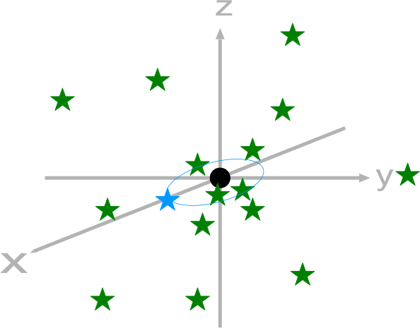
Figure 1 shows our numerical model schematically. The SMBH with its mass
 $M_{\rm SMBH}$
is set to the origin. The star symbols represent individual stars. Each of them is modeled by a point-mass particle. At the initial condition, the orbit of the particle representing S2 is in the x-y plane. We adopted the mass of the SMBH is
 $4.3\times 10^6 M_{\odot}$
, the initial semi-major axis of S2, a, is 125.058 mas (1030 AU adopting the distance to the GC,
 $R_0$
, as
 $8.2467$
kpc) and its initial eccentricity is 0.884649 (GRAVITY Collaboration 2020).
Schematic figure of our cluster model. As the structure of the star cluster at the initial condition, we adopted an
 $\eta$
-model proposed by Matsubayashi et al, (Reference Matsubayashi, Makino and Ebisuzaki2007), which is a dynamically stable stellar system model containing a massive object at its center.

The total mass of the star cluster,
 $M_{\rm total}$
, the enclosed mass within the apocenter of S2,
 $M_{\rm cl}$
, the number of star particles, N, are parameters which are summarized in Table 1Footnote †.
Parameters of selected models and runs reported in this manuscript. mass unit:
 $M_{\odot}$
.
 $n=1,5,10$
. We carried out
 $N_{\rm run }$
runs changing the seed for initial distribution of the star cluster in each model.

Table 1 Long description
A table comparing parameters of selected models and runs. The table has 4 rows and 8 columns. Column headers are ID, M_total, N_total, M_cl, m_star, m_star/M_MBH, M_IMBH, and N_run. Row 1: ID, m1-n; M_total, 6.394; N_total, nk; M_cl, 1.2; m_star, 63.26 n; m_star/M_MBH, 1.4847000/n x 10^-5; M_IMBH, -; N_run, 20. Row 2: ID, m2-n; M_total, 4.682; N_total, nk; M_cl, 0.88; m_star, 46.39 n; m_star/M_MBH, 1.0887000/n x 10^-5; M_IMBH, -; N_run, 20. Row 3: ID, m3-n; M_total, 2.979; N_total, nk; M_cl, 0.56; m_star, 29.52 n; m_star/M_MBH, 6.9286000/n x 10^-6; M_IMBH, -; N_run, 20. Row 4: ID, mi1-1; M_total, 6.394; N_total, 980; M_cl, 1.2; m_star, 63.26; m_star/M_MBH, 1.4847000 x 10^-5; M_IMBH, 1000; N_run, 20.
3. Method
We carried out a series of direct N-body simulations using GPLUM (Ishigaki et al. Reference Ishigaki, Kominami, Makino, Fujimoto and Iwasawa2021). GPLUM is a code developed to integrate an N-body system containing a gravitationally dominant object at its center, such as the Sun in the Solar System.
Numerical computations and analysis were carried out on PC cluster, Cray XC50 and analysis servers at the Center for Computational Astrophysics, National Astronomical Observatory of Japan.
4. Result
Here we show highlights of our work. More information will be presented in Funato & Makino (in prep.).
4.1 precession
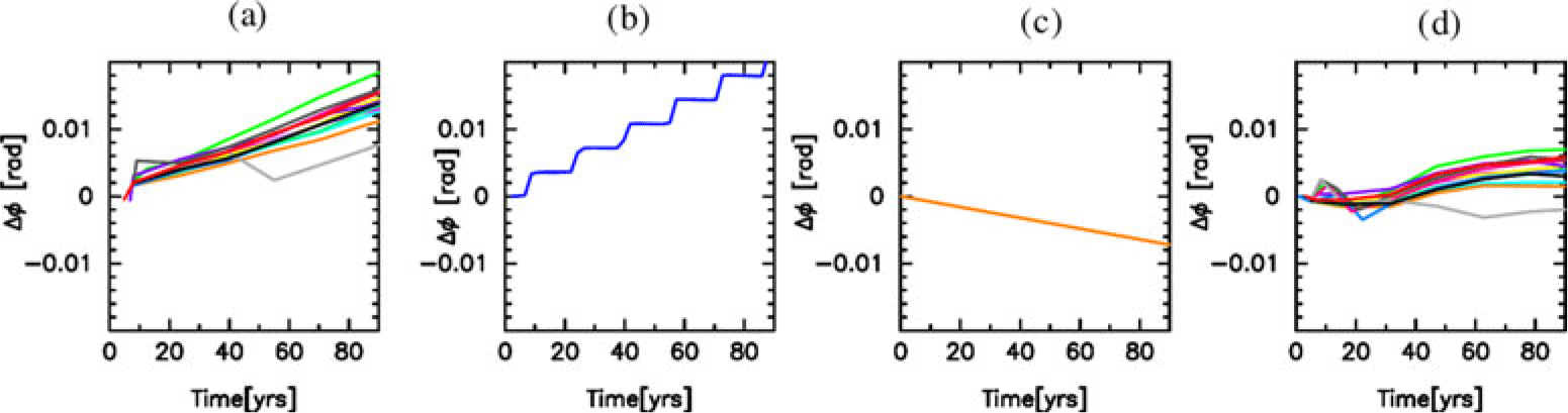
Figure 2(a) shows the time evolution of argument of periaps
 $\phi$
of S2. Each curve corresponds to each run in model1-1. Figures 2(b) and 2(c) show contributions of general relativistic effect (GR) and the mean field of the star cluster (MF) to change in precession, respectively. In Figure 2(d), shown is the residual after subtracting contributions of GR and MF. Figure 2(d) shows the contribution of RR. Though change due to RR exists, to estimate its contribution from observational data is complicated because of other two effects (GR and MF).
Change of argument of periaps. (a) observed (b) due to GR (c) due to MF (d) residual: (a)-(b)-(c).

4.2 inclination evolution
On the other hand, the effect of RR is clearly observed in the time evolution of inclination of S2. (It is sometimes called as Vector Resonant Relaxation (VRR)).
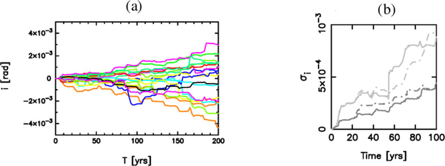
Figure 3(a) shows time evolution of inclination of each run of model m1-1. The change in inclination also increases/decreases linearly over time, as same as that in argument of periaps. Whether it increases or decreases depends on the bias of the initial particle distribution. For the axisymmetricity of the cluster model, there are no contribution from MF.
(a)Example of time evolution of inclination. (b)Comparison of time evolution of argument of
 $\sigma_{i}$
between w and wo GR effect.

In figure 3(b), we compare the time evolution of inclination between in the cases with GR and without GR. The curves in figure 3(b) show the time evolution of variance
 $\sigma_{i}$
. The light and dark gray curves correspond to the cases with models m1-1 and m1-5, respectively. The solid and dotted curves correspond to with and without GR, respectively. This figure shows that there is no effect of GR to the evolution of inclination. So in the following sections, we investigate the effect of RR from the point of view of evolution of inclination.
4.2.1 dependence on cluster properties
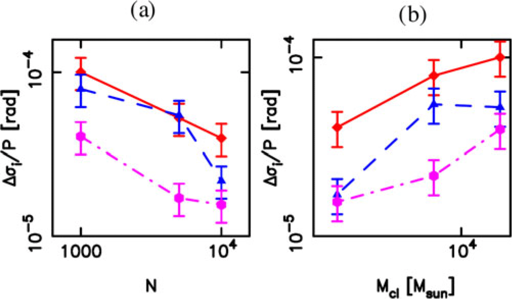
We summarize the dependence of growth rate of variance of inclination on cluster properties in Figure 4. Figure 4 shows the dependence is expressed as
 $\Delta\sigma_{\rm i}/P \propto M_{CL}N^{-1/2}$
. This is consistent with the prediction of Rauch & Tremaine (Reference Rauch and Tremaine1996).
The growth rate of variance of change of inclination per period is plotted against
 $M_{\rm cl}$
, which is the enclosed mass within the twice of apocenter of S2, and N. The solid, dashed and dot-dashed curves with filled-squares, filled-triangles and filled-circles (red, blue and magenta in electronical version) in Figure (a) correspond to a massive, middle and small cluster, respectively. Those in Figure (b) correspond to small, middle and large N, respectively.

4.2.2 Effect of Intermediate Mass Black Hole (IMBH)
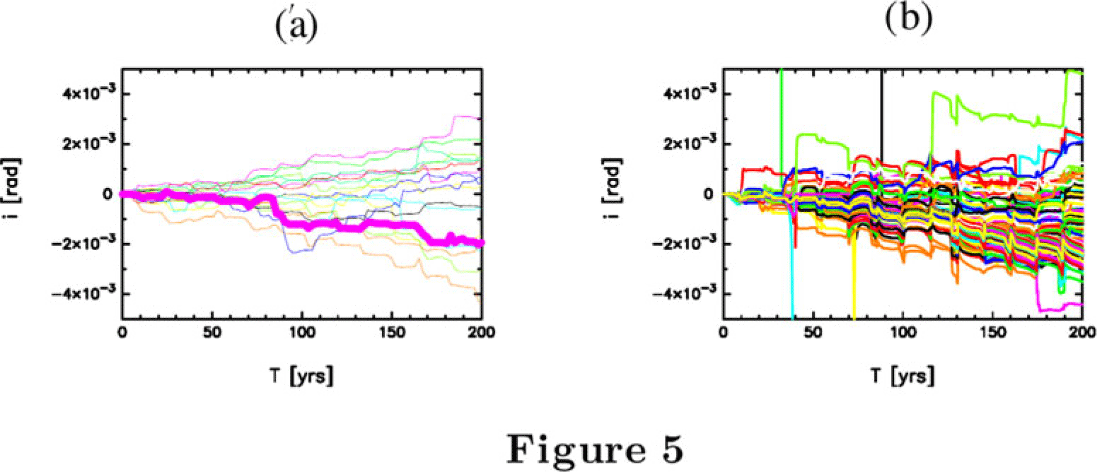
Figure 4 shows that time evolution of inclination. Each curve corresponds to the result of each run in model m1-1 (a) and mi1-1 (b). Note that figure 4(a) is the same figure as figure 3(a), but the width of curves is thin except for 1 run. As shown in Figure 4(a), in Figure 4(b) each curve increases/decreases linearly over time.
The difference between the curves in Figure 4 (a) is due to the difference in the distribution of particles at the initial condition. While that between the curves in Figure 4 (b) is due to the difference in the initial position and velocity of the IMBH particle at the initial condition. The distribution of other particles is the same as that of the run corresponding to the thick curve in Figure 4 (a).
Comparing Figures 4 (a) and (b), the increasing rate of variance
 $\sigma_{\rm i}$
seems almost the same in both figures.
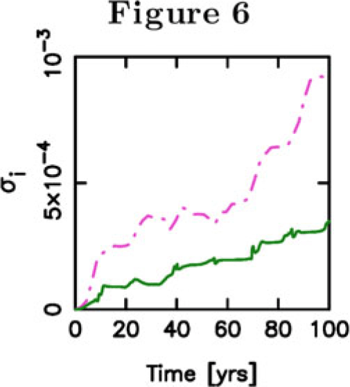
In Figure 6, we plotted time evolution of variance
 $\sigma_{\rm i}$
for the case with and without an IMBH. This figure shows that the time evolution of
 $\sigma_{\rm i}$
for the case with IMBH is in same order of that for the case without an IMBH. It is natural because RR is driven by the coherency of gravitational force from other objects. The effect of an IMBH can be equivalent to that of group of objects which is moving coherently and whose total mass is as same as that of the IMBH. But as shown in Figure 6, there is a difference of about a few times. At this point, the cause of this discrepancy is still unclear. It will be investigated in our future work.
Comparison of evolution of inclination of S2 between wo(a) and w(b) an IMBH. The spikes that appear about every 12 years are numerical errors rising at pericenter passage.

Time evolution of variance
 $\sigma_{\rm i}$
of inclination evolution. solid, dark (dark green in electronical version): with IMBH, dot-dashed, light (purple in electronical version): without IMBH.

5. Discussion
Our results suggest that for a population of equal-mass objects, the enclosed mass and N can be estimated from the evolution of the orbital inclinations of several S stars with similar apocenter distances. If the objects have a mass distribution, we need to be more careful. Even a single IMBH can have the same impact as a factor of difference in N or
 $M_{\rm cl}$
. It may be useful to consider the presence and mass of an IMBH with a different perspective (e.g., Gualandris & Merritt Reference Gualandris and Merritt2009).
 η

 M⊙
 n=1,5,10
 Nrun
 σi
 Mcl
 σi

 Open access

